Electroweak phase transition in the scotogenic model

Abstract

In this work we study the behavior of the effective scalar potential at zero and finite temperature of the scotogenic model. In particular, we analyze the impact of the Yukawa couplings associated to the right–handed neutrinos on the electroweak phase transition.

1 Introduction

The need for physics beyond the Standard Model (SM) arises from experimental evidence of at least three phenomena with no support within the SM framework: neutrino masses, dark matter (DM) and the matter–antimatter asymmetry. Along this lines, Ernest Ma [1] proposed the scotogenic model, that radiatively generates neutrino masses and has a viable DM candidate. On the other hand, the matter–antimatter asymmetry can be explained from two general approaches: baryogenesis via leptogenesis [2] and electroweak baryogenesis (EWB) [3]. Sakharov [4] set three conditions for any model that attempts to explain the baryon asymmetry: i) baryon number violation, ii) CP violation and iii) departure from thermal equilibrium. In this work we will only focus on the third condition. Within EWB, the departure from equilibrium is achieved through a strong first–order electroweak phase transition (EWPT) and the baryon number preservation condition (BNPC) of the effective scalar potential. Thus, the aim of this work is to show how is the behaviour of the scalar potential of the scotogenic model when quantum and thermal corrections are taken into account; in particular, when the Yukawa couplings leading to neutrino masses are non negligible.

2 The model and thermal corrections

The scotogenic model is an extension of the SM with a second Higgs doublet $\Phi$, three right-handed neutrinos, $N_{i}$ ($i=1,2,3$), and a $Z_{2}$ symmetry such that the SM fields are even and the new fields are odd. The right–handed neutrino interactions with SM particles are given by:

$$\mathcal{L}_{int}=-h_{ij}\overline{N_{R}^{i}}\tilde{\Phi}^{\dagger}\ell^{j}_{L}+\text{h.c.}\quad\text{($\tilde{\Phi}=i\sigma_{2}\Phi^{*}$)}.$$ (1)

On the other side, the scalar interactions of the model can be expressed via the scalar potential [5]:

$$V_{0} = \mu^{2}_{1}|H|^{2}+\mu^{2}_{2}|\Phi|^{2}+\lambda_{1}|H|^{4}+\lambda_{2}|\Phi|^{4}+\lambda_{3}|H|^{2}|\Phi|^{2}+\lambda_{4}|H^{\dagger}\Phi|^{2}$$ (2)

$$+ \frac{\lambda_{5}}{2}\left[(H^{\dagger}\Phi)^{2}+\text{ h.c.}\right],$$

where the doublets are

$$H=\begin{pmatrix}G^{\pm}\\ \frac{1}{\sqrt{2}}(v+h+iG^{0})\end{pmatrix},\quad\Phi=\begin{pmatrix}H^{\pm}\\ \frac{1}{\sqrt{2}}(\phi+H^{0}+iA^{0})\end{pmatrix},$$ (3)

being $v$ and $\phi$ the vev of $H$ and $\Phi$, respectively, and $H^{0}$ is the DM candidate (for this work). In the most DM models, the $Z_{2}$ symmetry remains unbroken to ensure stability of the DM candidate. In this work, we will relax that condition and allow $Z_{2}$ can develop a vev.

The effective potential and thermal corrections

The thermal corrections are included through the effective scalar potential:

$$V_{eff}(v,\phi,T)=V_{0}+V_{1}(v,\phi)+V_{T}(v,\phi,T),$$ (4)

where $V_{0}$ is the tree level scalar potential, $V_{1}(v,\phi)$ is the one loop correction to (2) at zero–temperature (Coleman–Weinberg potential) and $V_{T}(v,\phi,T)$ represents the thermal and ring contributions [6]:

$$V_{1}(v,\phi)=\sum_{i\,={\text{ all fields}}}\frac{n_{i}m_{i}^{4}(v,\phi)}{64\pi^{2}}\left[\ln{\frac{m^{2}_{i}(v,\phi)}{Q^{2}}}-c_{i}\right],$$ (5)

$$V_{T}(v,\phi,T) = \frac{T^{4}}{2\pi^{2}}\left\{\sum_{B}n_{i}J_{B}\left[\frac{m_{i}^{2}(v,\phi)}{T^{2}}\right]+\sum_{F}n_{i}J_{F}\left[\frac{m_{i}^{2}(v,\phi)}{T^{2}}\right]\right\}$$ (6)

$$+ \sum_{i\,={\text{ all fields}}}\frac{T}{12\pi}\left(\frac{1+\varepsilon}{2}\right)n_{i}\left\{\left[m_{i}^{2}(v,\phi)\right]^{3}-\left[m_{i}^{2}(v,\phi,T)\right]^{3}\right\},$$

where $B$ stands for scalars and bosons, and $F$ for fermions. The thermal functions are expressed as:

$$J_{B}[y^{2}]=\int_{0}^{\infty}dx\ x^{2}\log\left[1-e^{-\sqrt{x^{2}+y^{2}}}\right],\quad J_{F}[y^{2}]=\int_{0}^{\infty}dx\ x^{2}\log\left[1+e^{-\sqrt{x^{2}+y^{2}}}\right].$$ (7)

In this case, $n_{i}$ are [5] $n_{Z}=3$, $n_{W}=6$, $n_{t}=-12$, $n_{h}=1$, $n_{G^{0}}=1$, $n_{G^{\pm}}=2$, $n_{H^{\pm}}=2$, $n_{H^{0}}=1$, and $n_{A^{0}}=1$. The $c_{i}$ coefficients are established by the nature of the fields: $3/2$ for scalars and fermions and $5/6$ for gauge bosons. The factor $\varepsilon$ is $1$ for bosons and $-1$ for fermions, and $Q$ is the renormalization scale.

Masses of the model

The field dependent masses, $m_{i}$, are determined by a diagonalization process of the following matrices [5]:

$$M^{2}_{h}=\begin{pmatrix}\mu_{1}^{2}+3\lambda_{1}v^{2}+\lambda_{L}\phi^{2}&2\lambda_{L}\phi v\\ 2\lambda_{L}\phi v&\mu_{2}^{2}+3\lambda_{2}\phi^{2}+\lambda_{L}v^{2}\end{pmatrix},\quad M^{2}_{A}=\begin{pmatrix}\mu_{1}^{2}+\lambda_{1}v^{2}+\lambda_{S}\phi^{2}&\lambda_{5}\phi v\\ \lambda_{5}\phi v&\mu_{2}^{2}+\lambda_{2}\phi^{2}+\lambda_{S}v^{2}\end{pmatrix},$$

$$M^{2}_{\pm}=\begin{pmatrix}\mu_{1}^{2}+\lambda_{1}v^{2}+\frac{1}{2}\lambda_{3}\phi^{2}&\frac{1}{2}(\lambda_{5}+\lambda_{4})\phi v\\ \frac{1}{2}(\lambda_{5}+\lambda_{4})\phi v&\mu_{2}^{2}+\lambda_{2}\phi^{2}+\frac{1}{2}\lambda_{3}v^{2}\end{pmatrix},$$ (8)

with $\lambda_{L}=(\lambda_{3}+\lambda_{4}+\lambda_{5})/2$ and $\lambda_{S}=(\lambda_{3}+\lambda_{4}-\lambda_{5})/2$. For the thermal corrections, the masses resulting from the diagonalization process of (2) contain the $\mu_{i}$ parameters. Thus, the thermal corrections require that $\mu^{2}_{i}\longrightarrow\mu^{2}_{i}+c_{i}T^{2}$ [5, 7], where

$$c_{1}=\frac{1}{8}g^{2}+\frac{1}{16}(g^{2}+g^{\prime 2})+\frac{1}{2}\lambda_{1}+\frac{1}{12}(\lambda_{L}+\lambda_{S})+\frac{1}{12}\lambda_{3}+\frac{1}{4}y_{t}^{2},\quad\text{(SM fields)}$$ (9)

$$c_{2}=\frac{1}{8}g^{2}+\frac{1}{16}(g^{2}+g^{\prime 2})+\frac{1}{2}\lambda_{2}+\frac{1}{12}(\lambda_{L}+\lambda_{S}+\lambda_{3})+\frac{9}{12}h^{2}_{\nu}.\quad\text{(new fields)}$$ (10)

being $g$ and $g^{\prime}$ the electroweak couplings, $y_{t}$ the Yukawa top coupling and $h_{\nu}$ are given by

$$h_{\nu}=\frac{1}{3}\sqrt{\sum_{i,j}|h_{ij}|^{2}}.$$ (11)

Note that the $h_{\nu}$ couplings contribute to the thermal masses of the new fields (see equation (10)) in opposition to the inert double model (IDM) case [5]. For gauge bosons, only longitudinal components get thermal masses given by the eigenvalues of

$$\begin{pmatrix}\frac{1}{4}(v^{2}+\phi^{2})g^{2}+2g^{2}T^{2}&-\frac{1}{4}(v^{2}+\phi^{2})gg^{\prime}\\ -\frac{1}{4}(v^{2}+\phi^{2})gg^{\prime}&\frac{1}{4}(v^{2}+\phi^{2})g^{\prime 2}+2g^{\prime 2}T^{2}\end{pmatrix},$$ (12)

while for $W$ the contribution is $m^{2}_{W_{l}}=m^{2}_{W_{l}}(v,\phi)+2g^{2}T^{2}.$

3 Numerical analysis and results

For numerical analysis the masses and couplings are fixed as follows: $m_{H^{0}}=66$ GeV (low DM mass regime), $m_{H^{\pm}}$ and $m_{A^{0}}$ greater than $200$ GeV (with $m_{H^{\pm}}=m_{A^{0}}$), $\lambda_{L}=\lambda_{2}=0.01$ and $h_{\nu}=0.31,1.0,1.73$. The scale $Q$ is fixed at electroweak symmetry breaking scale, that is $Q=246.22$ GeV.

Limits for $m_{H^{\pm}},m_{A^{0}}$ masses

At zero temperature, the effective scalar potential of the model (4) must exhibit the usual behaviour of the SM, i.e., the global minimum of the system must be associated with the electroweak symmetry breaking. This imposes limits on the masses of $m_{H^{\pm}}$ and $m_{A^{0}}$.

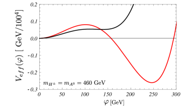
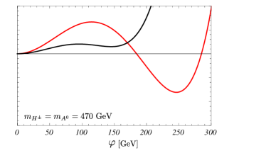
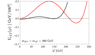
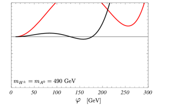
Figure 1: Effective potential behaviour at $T=0$ GeV when $m_{H^{0}}=66$ GeV and different values of $m_{H^{\pm}}=m_{A^{0}}$. The red line indicates $V_{eff}(\varphi)=V_{eff}(v,0,0)$ and black line indicates $V_{eff}(\varphi)=V_{eff}(0,\phi,0)$.

As we can see in Figure 1, the behaviour of $V_{eff}(v,\phi,0)$ is related with the values of $m_{H^{\pm}}$ and $m_{A^{0}}$. For $m_{H^{\pm}}=m_{A^{0}}=460$ GeV, the effective potential $V_{eff}(v,0,0)$ (red line in Figure 1) have a deeper global minimum respect $V_{eff}(0,\phi,0)$ (black line in Figure 1). Thus the phenomenology of the model is associated to SM phenomenology. As the value of the masses increases, this global minimum begins to rise while $V_{eff}(0,\phi,0)$ begins to sink. However, when $m_{H^{\pm}}=m_{A^{0}}=490$ GeV, the global minimum of the effective potential is lost with the $Z_{2}$ symmetry breaking, which cannot be possible because the SM phenomenology. So, in order to preserve the electroweak symmetry breaking, the masses of $m_{H^{\pm}}$ and $m_{A^{0}}$ GeV are set at 460 GeV hereafter.

EWPT

One of the main conditions needed to have a strong first-order EWPT is the BNPC, which requires that $R\equiv v_{C}/T_{C}>1,$ [5], where the critical temperature $T_{C}$ is the temperature at which the potential (4) has two degenerate minima (for different values of the SM vev), and $v_{C}$ is the non-zero vev of the broken phase at the critical temperature. For $m_{H^{\pm}}=m_{A^{0}}=460$ GeV and $h_{\nu}=0.31$, the effective potential exhibits a strong first–order EWPT at a critical temperature of $T_{C}=90.8$ GeV when $v_{C}=242.92$ GeV (and therefore $R=2.67$), as it is shown in left panel of Figure 2 (red solid line).

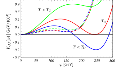
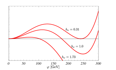
Figure 2: Left: effective potential behaviour for different temperature values and $h_{\nu}=0.31$. The solid lines indicate $V_{eff}(\varphi)=V_{eff}(v,0,T)$ and the dashed lines indicate $V_{eff}(\varphi)=V_{eff}(0,\phi,T)$. Right: effective potential behaviour at $T=90.8$ GeV, $m_{H^{0}}=66$ GeV and $m_{H^{\pm}}=m_{A^{0}}=460$ GeV for different values of $h_{\nu}$.

The interesting thing about this benchmark point is that the $Z_{2}$ symmetry is not affected by the thermal corrections and never develops a second minimum deeper than the SM one. Therefore, the DM candidate is still stable.

Impact of the Yukawas on the effective potential

Another interesting aspect is the dependence of the effective potential with the Yukawa couplings $h_{\nu}$. From the right panel of Figure 2, it is clear that the strong first–oder EWPT only occurs when the Yukawa couplings are set to $h_{\nu}=0.31$. Moreover, we found that for $h_{\nu}=1.0$ the EWPT is still strong and first order but with a higher critical temperature $T^{\prime}_{C}=129.8$ GeV at $v^{\prime}_{C}=244.3$ GeV ($R^{\prime}=1.89$). Whereas for $h_{\nu}=1.73$, the behaviour of the scalar effective potential changes and therefore it is not possible to have strong first–order EWPT.

4 Conclusions

The scotogenic model allows us to establish the minimum conditions to explain two of the phenomena that the SM is not able to explain given the current data. However, may have one of the requirements to address a third phenomena: the baryon asymmetry. In this work we have studied the EWPT and BNPC in the scotogenic model through the effective scalar potential. Taking into account only the Coleman–Weinberg potential ($T=0$), we can set a limit of $m_{H^{\pm}}=m_{A^{0}}=460$ GeV for the validity of SM. When the thermal corrections of the effective potential and masses of the fields are considered, the Yukawa coupling values have a strong impact on the behaviour of the effective potential. When the DM candidate has a mass of $m_{H^{0}}=66$ GeV, $m_{H^{\pm}}=m_{A^{0}}=460$, and $h_{\nu}=0.31$, the effective potential exhibits a strong first–order EWPT and the BNPC is satisfied. However, for the same benchmark point and larger values of $h_{\nu}$, the strong first–order EWPT and BNPC are only present when $h_{\nu}=1.0$ for a critical temperature such that $T^{\prime}_{C}>T_{C}$ (and $R^{\prime}<R$). Consequently, a strong first–order EWPT will be present only if $h_{\nu}\leqslant 1.0$ for the scotogenic model.

References

• [1] E. Ma, “Verifiable radiative seesaw mechanism of neutrino mass and dark matter,” Phys. Rev., Vol. D73, p. 077301, 2006.
• [2] A Strumia. “Baryogenesis via leptogenesis”, In Particle physics beyond the standard model, proceedings, Summer School on Theoretical Physics, 84th Session, Les Houches, France, August 1-26, 2005, pages 655–680, 2006.
• [3] D. Morrissey & M. J. Ramsey–Musolf, “Electroweak baryogenesis”. New J. Phys., 14:125003, 2012.
• [4] A. D. Sakharov, “Violation of CP Invariance, c Asymmetry, and Baryon Asymmetry of the Universe”, Pisma Zh. Eksp. Teor. Fiz., Vol. 5, pp. 32–35, 1967.
• [5] N. Blinov, S. Profumo, and T. Stefaniak, “The Electroweak Phase Transition in the Inert Doublet Model”, JCAP, Vol. 1507, no. 07, p. 028, 2015.
• [6] J. R. Espinosa & M. Quirós, “Novel effects in electroweak breaking from a hidden sector”, Phys. Rev. D, Vol. 76, pp. 076004–1, 2007.
• [7] A. Merle & M. Platscher, “Parity Problem of the Scotogenic Neutrino Model”, Phys. Rev., Vol. D92, no. 9, p. 095002, 2015.