The Mass-to-light Ratios and the Star Formation Histories of Disk Galaxies

Abstract

We combine new data from the main sequence ($M_{*}$ versus SFR) of star-forming galaxies and galaxy colors (from $GALEX$ to $Spitzer$) with a flexible stellar population scheme to deduce the mass-to-light ratio ($\Upsilon_{*}$) of star-forming galaxies from the SPARC and S⁴G samples. We find that the main sequence for galaxies, particular the low-mass end, combined with the locus of galaxy colors, constrains the possible star formation histories of disk and dwarf galaxies to a similar shape found by Speagle et al. (2014). Combining the deduced star formation history with stellar population models in the literature produces reliable $\Upsilon_{*}$ values as a function of galaxy color with an uncertainty of only 0.05 dex. We provide prescriptions to deduce $\Upsilon_{*}$ for optical and near-IR bandpasses, with near-IR bandpasses having the least uncertainty ($\Upsilon_{*}$ from 0.40 to 0.55). We also provide the community with a webtool, with flexible stellar population parameters, to generate their own $\Upsilon_{*}$ values over the wavelength range for most galaxy surveys.

1 Introduction

With the discovery of the radial acceleration relation (McGaugh, Lelli & Schombert 2016), it has become increasingly obvious that, on galactic scales, baryons play a dominant role in the formation and evolution of galaxies. The baryonic component of galaxies is primarily gas (atomic, molecular and ionized) and stars (visible and remnants). The gaseous component in galaxies is heavily dominated by atomic gas (e.g, Cortese, Catinella & Janowiecki 2017), which is well measured using HI observations and corrected by a factor of 1.33 to account for He and molecular components. The stellar baryon component is estimated from determination of the total luminosity of a galaxy (at different wavelengths), then converted into a total stellar mass value through multiplication of a mass to light ratio ($\Upsilon_{*}$), a value deduced through some knowledge of the star formation history of the galaxy.

In addition to probing the star formation history of a galaxy, a detailed knowledge of the $\Upsilon_{*}$ is also a critical test for exotic theories such as MOND (MOdified Newtonian Dynamics) and emergent gravity. MOND proposes that the equations of motion become scale-invariant at accelerations smaller than a characteristic acceleration scale ($a_{o}=cH_{o}/6$, Milgrom 2009). It predicts a correlation between the observed centripetal acceleration and the acceleration from baryons (for a typical rotating galaxy, this is due to gas and stars, thus the need for $\Upsilon_{*}$ to convert luminosity into stellar mass). Emergent gravity proposes that gravity is not a fundamental force but emerges from an underlying microscopic theory (Verlinde 2016). It requires particular values of $\Upsilon_{*}$ in order to accommodate the observed acceleration for a range of galaxy sizes (Lelli, McGaugh & Schombert 2017).

To calculate the stellar mass of a galaxy ($M_{*}$) one requires 1) an accurate value for the total stellar luminosity of a galaxy ($L_{tot}$) plus 2) a reliable $\Upsilon_{*}$ at the same wavelength that the luminosity is determined. While photometry of galaxies still contains many inherent uncertainties (different aperture sizes, foreground stars, nearby companion galaxies), the advent of areal detectors and space imaging (where the sky brightness is substantially fainter) has removed most of the limitations to assigning an accurate total luminosity to galaxies (i.e., an well defined curve-of-growth to the galaxy’s luminosity profile). Detailed surface photometry also allows for a determination of the stellar luminosity per parsec² and allows pixel-by-pixel evaluation of the underlying stellar population (see Lee et al. 2018). Thus, the uncertainties in stellar luminosity can be estimated by various methods, but evaluating the reliability of an $\Upsilon_{*}$ is more difficult due to the convolved path of stellar population modeling that is involved in deducing the appropriate $\Upsilon_{*}$ at the wavelength of interest.

Two advances in recent years has dramatically improved our ability to deduce stellar mass from photometry. The first is the increased sophistication in the suite of stellar isochrones used to produce stellar population models that allows inspection of the effects of exotic components, such as horizontal branch and blue straggler stars, as well as more detailed understanding of the effects of dust and the IMF. In addition, there is recent awareness that detailed SED fitting is not critical to deducing $\Upsilon_{*}$ from population models, so that broadband photometry is adequate (Gallazzi & Bell 2009) as long as sufficient wavelength coverage is obtained. With this technique, one determines $\Upsilon_{*}$ through various mass-to-light versus color relations (MLCR) as well as from detailed spectral indices, a procedure that is laced with complications (see McGaugh & Schombert 2014).

These improvements are well timed with the second advance on the observational side, increasing numbers of nearby galaxies with detailed color-magnitude diagrams (CMD’s) of the resolved stellar populations plus improved photometry in the UV and near-IR (i.e., $GALEX$ and $Spitzer$). CMD’s in nearby galaxies allow for direct comparison between stellar population models and the actual stellar content. The new observations in the UV serve to constrain recent star formation rates, while new near-IR observations provide more reliable luminosities to deduce $\Upsilon_{*}$ (as $\Upsilon_{*}$ variations decrease significantly in the near-IR where old stars dominate the baryonic mass, Rix & Zaritsky 1995; Norris et al. 2016).

For star-forming galaxies, a valid $\Upsilon_{*}$ estimate requires two components, 1) a reasonably constrained star formation history (knowledge of the change in the star formation rate and chemical enrichment with time) and 2) reliable stellar population models as a function of age and metallicity (to deduce how luminosities, as a function of color, are converted into mass). While it is straight forward to test stellar population models against star clusters (Bruzual 2010) or quiescent galaxies, like ellipticals (Schombert 2016), it is much more problematic to attempt to extract colors and $\Upsilon_{*}$ from star-forming galaxies such as spirals and dwarf irregulars (Bell & de Jong 2000) due to the competing drivers of star formation and chemical enrichment.

There are two core observables for star-forming galaxies that can constrain their complex histories and assist in deriving a stable $\Upsilon_{*}$’s; 1) the galaxy mass versus SFR (star formation rate) diagram (the so-called main sequence for star-forming galaxies, MSg, Noeske et al. 2007; Speagle et al. 2014) and 2) the locus of galaxy’s colors, particularly optical versus IR colors. The MSg allows a crude description of the star formation history (SFH); for most high-mass galaxies lie near the region of gas exhaustion (meaning their past SFR must have been much higher than the present), while low-mass galaxies lie near the line of constant SFR, meaning their past SFR’s must be near the current one (see Figure 1). This highly constrains the possible paths of past star formation as any past star formation (SF) must be near the current SFR (although one can entertain many scenarios, such as late formation epochs, see §4).

In addition to the MSg, the suite of galaxy colors has also dramatically increased, not only in number but in the range of wavelength’s sampled. Our focus, for this study, is on the SPARC (Spitzer Photometry and Accurate Rotation Curves, Lelli, McGaugh & Schombert 2016) and S⁴G (Sheth et al. 2010) datasets, as they have the fullest coverage at 3.6$\mu$m, the $Spitzer$ channels, which are of highest interest in deducing $\Upsilon_{*}$. For a subset of several hundred galaxies in these two samples, there is photometry from $GALEX$ $FUV$ to $Spitzer$ 4.5$\mu$m, including optical ($SDSS$, RC3) and near-IR ($2MASS$, $WISE$). The colors presented herein are total colors, i.e., deduced from total luminosities in the various bandpasses.

The goal of this project is to combine new information from these color/SFR relations, plus refined stellar population models, to obtain new color-$\Upsilon_{*}$ relations over a broad range of colors and stellar masses. Our emphasis is on the near-IR colors due their importance to the SPARC project (Lelli et al. 2017), however, the models are applicable to a range of galaxy colors and are flexible to a range of input parameters, such as different star formation histories and paths of chemical evolution.

2 Main Sequence Relationship for Star-forming Galaxies

The main sequence for star-forming galaxies (where the designation of star-forming includes, basically, all Hubble types later than Sa) is a somewhat surprising relationship for galaxies since color and SFR vary widely with morphology suggesting complicated star formation histories. Considerable recent work has been motivated by more accurate stellar mass determinations (using near-IR luminosities) and has focussed on the star-forming main sequence through a direct comparison of the total stellar mass of a galaxy versus its current SFR (Noeske et al. 2007; Salim et al. 2007; Daddi et al. 2007; Peng et al. 2010; Wuyts et al. 2011; Cook et al. 2014; Speagle et al. 2014; Jaskot et al. 2015; Cano-Diaz et al. 2016; Kurczynski et al. 2016). The two parameters are clearly indirectly connected as the total stellar mass of a galaxy reflects the integrated SFR over the complete SFH of the galaxy (or reflects the SFH of the merger progenitors). However, the current SFR only reflects the last stage of an unknown, and possibly very complex, star formation history. If star formation has been a uniform process, then the current SFR presumingly scales with the mean SFR of the galaxy and, thus, its integrated value becomes the total stellar mass. A correlation between the current SFR value and total stellar mass, and its narrowness, implies continuous evolution (Noeske et al. 2007) with roughly uniform, ongoing SF during this time. While the SFH’s may have a range of shapes (e.g., on and off bursts), the continuous consumption of gas implies that the evolution of SFR with time must also be relativity similar across the various galaxy types (see also Abramson et al. 2016).

We note that using the MSg to deduce $\Upsilon_{*}$ is somewhat circular, as total stellar mass is deduced from total stellar luminosity, which we will then use to constrain the value of $\Upsilon_{*}$ from stellar population models. However, the stellar mass axis is linear to changes in $\Upsilon_{*}$ and small changes to the total stellar mass alters the integral value of the SFH. Most of the observational error is in the SFR values, and changes in the final SFR on the shape of the SFH has a larger impact to the total stellar mass.

The term "main sequence" for galaxies is a poor analogue with the main sequence of stars, which is driven by some basic nuclear physics, and the relationship between stellar mass and current star formation (SF) has many competing processes to enhance or suppress SF leading to complex histories behind the observed final outcome. However, there are some interesting similarities. For example, the MSg relationship is well defined with relatively low scatter on the low-mass end (Cook et al. 2014), defined by the slowly evolving galaxies. Considering the high gas fractions, typical for low-mass LSB galaxies, this is surprising as one could imagine discontinuous sharp bursts of SF (although not in line with their low stellar density appearances). As one goes to higher stellar masses (lower gas fractions) the relationship displays a "turn-off" at $M_{*}\approx 10^{10}M_{\sun}$ suggesting a point where gas depletion occurs on timescales less than the age of the Universe ("weary giants", see McGaugh, Schombert & Lelli 2017). The low-mass end contains the "thriving dwarfs" with their plentiful gas supplies.

The main sequence relation plays a more important role when followed over redshift as it then represents the SFR as a function of time per mass bin. This has been successfully applied by Speagle et al. (2014), who uses the change in the zeropoint of the MSg to deduce an average SFH for galaxies (see their Figure 9). That study, notably, finds the slope of the MSg to vary only slightly with cosmic epoch and defines the canonical fit for the current epoch ($z=0$) by extrapolation to the current epoch. However, the fitted slope of the relation on the high-mass end varies from rather flat at low redshift ($z=0.2$, Speagle et al. 2014) to rather steep at high redshifts ($z=0.9$, Kurczynski et al. 2016). We will use the shape of the extrapolated $z=0$ SFH as the baseline shape of SFH for our analysis in §4 (i.e., an initial burst with a slowly declining SFR to the present epoch). We make one small adjustment to the Speagle et al. SFH prescription in that we set the initial epoch of star formation at 1 Gyr after the BB, rather than 4. We find the linear extrapolation from Speagle et al. Figure 9 to be in good agreement with our own SPARC H$\alpha$ dataset (Lelli et al. 2016). Nearly all the high-mass spirals must follow some variation of this basic scenario in order to explain their positions on the main sequence.

However, the Speagle et al. (and most MSg studies) focus, primarily, on the high-mass end, rarely fitting below $10^{9}$ $M_{\sun}$ (due to luminosity limitations of high redshift samples). On the low-mass end, a much steeper slope is found near a value of 1 (Cook et al. 2014; McGaugh, Schombert & Lelli 2017). The data from Cook et al. (2014) and the LSB+SPARC (a combination of our $Spitzer$ studies of low surface brightness dwarfs plus the SPARC galaxies) dataset are shown in Figure 1 along with the fits from McGaugh, Schombert & Lelli (2017) plus the $z=0$ fit from Speagle et al. (their equation 28). A similar fit for low-mass disks was found by Medling et al. (2018), confirming the downward turn of the MSg below log $M_{*}$ = 10. The data is also flagged for $FUV-NUV$ color, where $GALEX$ data was available. In addition, the line of constant SFR for the age of the Universe (i.e., SFR $\approx M_{*}/t_{G}$ for $t_{G}$ = 13 Gyrs) is also indicated for reference.

The advantage of the Cook et al. and LSB+SPARC datasets is that each determined the current SFR by different methods. The LSB+SPARC dataset used traditional H$\alpha$ observations to determine the current SFR using the canonical H$\alpha$-to-SFR conversion of Kennicutt & Evans (2012). The Cook et al. sample used the $FUV$ flux of a galaxy converted to the current SFR through the prescription of Murphy et al. (2011). For galaxies in common (15), they have a good one-to-one correspondence between the deduced SFR, despite sampling slightly different timescales of SFR. We note that for the lowest mass galaxies, with log SFR $<-4$, that this corresponds to a current SFR that is barely measurable (a single O star powered HII region). At log SFR = $-5$, the SFR is down to a single B star. The $FUV$ flux is a better indicator of SFR in the extremely low SFR realm since it covers a timescale of 100 Myrs and is not dependent on the H$\alpha$ emission from short-lived (20 Myrs) O star complexes. In either case, it is our opinion, that observed SFRs below $10^{-4.5}$ are extremely inaccurate.

Two features are notable. First, some downward extension below $M_{*}<10^{10}$ M_☉ is expected as the line of constant SFR intersects the Speagle et al. relationship at that stellar mass. But the Speagle et al. sequence for the weary giants clearly deviates at $10^{10}$ $M_{\sun}$ from the slope defined by the Cook and LSB+SPARC samples. This is the region proposed by Peng et al. (2010) as the transition from merger quenching versus mass quenching (a term to signify the many feedback mechanisms that regulate/halt star formation). Environmental effects also begin to have a significant effect above this mass range (Speagle et al. 2014) plus gas exhaustion, or strangulation, begins to flatten the main sequence above $10^{10}M_{\sun}$ (Peng et al. 2015; McGaugh, Schombert & Lelli 2017).

Second, the low-mass galaxies can be divided by their $FUV-NUV$ color, with the bluer UV color galaxies having higher current SFR than the redder galaxies. This divide also occurs across the constant SFR line, signaling that galaxies with blue $FUV-NUV$ have rising SFR’s (at least in the last 100 Myrs, the timescale measured by the $FUV$ flux) and red galaxies have declining SFR’s in the last 100 Myrs. Again, episodic star formation can produce any total stellar mass and a broad range in current SFR. The fact that low-mass dwarfs display a coherence in the last phase of SFR with their position on the main sequence suggests a smooth, uniform SFH.

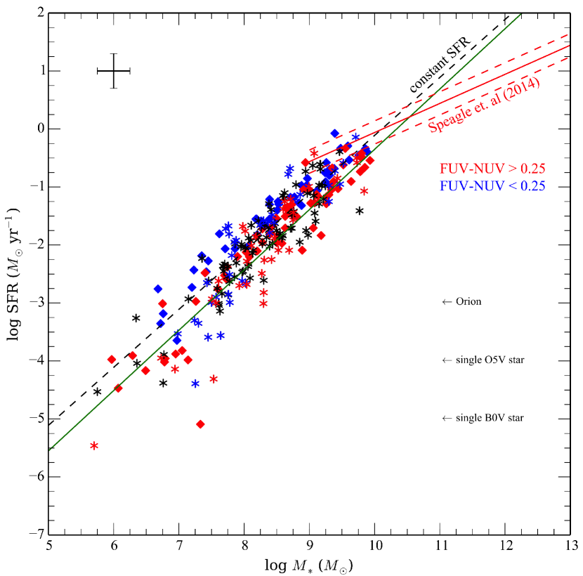
Figure 1: The main sequence for high and low-mass star-forming galaxies. The datasets from Cook et al. (solid symbols) and LSB+SPARC (starred symbols) are shown, color coded by $FUV-NUV$ color. The green line is a fit to the LSB+SPARC sample (McGaugh, Schombert & Lelli 2017). The dashed line is the line of constant star formation for a 13 Gyr Universe. There is a clear trend for blue $FUV-NUV$ colors to lie above the constant SFR line (rising SFR in the last 100 Myrs) versus red $FUV-NUV$ colors below the line (declining SFH). The $z=0$ relationship from Speagle et al. is shown for the high-mass spirals, along with 3$\sigma$ boundaries. Also shown are the values for SFR that correspond to an Orion-sized complex, a single O star and a single B star. SFR estimates below $-$4.5 are highly inaccurate. A representative error is shown in the upper left, errors in SFR and stellar mass are from McGaugh, Schombert & Lelli (2017).

3 Star-Forming Galaxy Colors

The history of multi-color photometry of galaxies is lengthy (see Schombert 2018) with the ultimate goal of using colors to untangle the underlying stellar populations in galaxies. While this has been successful for ellipticals, due to their simpler SFH’s and stellar populations colors dependent primarily on metallicity (Schombert 2016), star-forming galaxies present a more complicated interpretation of their colors as age (i.e., SF) plays a dominant role. Rather than attempting to deduce the exact metallicity and age of the stellar populations in star-forming main sequence galaxies (such as Bell & de Jong 2000), a more promising path is to use their colors to constrain the possible scenarios of star formation that produce their location on the observed main sequence. This allows an interpretation of $\Upsilon_{*}$, deduced from stellar population models, as a function solely of galaxy color, with some understanding of the scatter in $\Upsilon_{*}$ introduced by star formation assumptions and folding variables, such as age and metallicity, into the integrated colors.

The relevant colors for star-forming galaxies, that impact on deducing their SFH’s, can be divided into UV (short of 3500Å), optical (from 3500 to 5500Å) and near-IR (beyond 3 microns) colors. There are numerous sources for optical colors ranging from recent SDSS studies (Smolcic et al. 2006) to the RC3 (de Vaucouleurs et al. 1991). The UV is dominated by results from $GALEX$ ($FUV$ and $NUV$, Morrissey et al. 2007). The near-IR is sampled by $2MASS$ (Jarrett et al. 2000), $WISE$ (Wright et al. 2010) and $Spitzer$ (Schombert & McGaugh 2014). For the purposes of exploring the behavior of $\Upsilon_{*}$, $Spitzer$ 3.6$\mu$m data is preferred as it is farthest to the red without encountering contamination by PAH emission.

With the focus on $Spitzer$ 3.6$\mu$m photometry, we have also collected photometry from the S⁴G survey (Sheth et al. 2010) and combined this sample with our own LSB+SPARC survey (Lelli, McGaugh & Schombert 2016) and $FUV$ photometry from Cook et al. (2014). $Spitzer$ photometry was reevaluated for all three samples using direct surface photometry of the images in the $Spitzer$ archive (see Schombert & McGaugh 2014 for description of the reduction pipeline). After culling for photometric accuracy (all galaxies had to have $Spitzer$ magnitude errors less than 0.3), 301 galaxies were extracted from the S⁴G sample, 120 were extracted from Cook et al. and 160 were extracted from the LSB+SPARC dataset. Optical colors were extracted from NED using a variety of sources plus our own optical photometry of LSB galaxies in the SPARC sample (Pildis, Schombert & Eder 1997). The optical to near-IR colors were made by comparing NED aperture magnitudes to the full curve of growth in the $Spitzer$ photometry (using the largest aperture in NED). A comparison to SDSS DR14 images was made for the SPARC dataset (see Schombert 2016) to confirm the NED optical values. All magnitudes were corrected for Galactic extinction.

These three samples are displayed in Figure 2, corrected for internal extinction (following the standard RC3 correction based on galaxy type and inclination) and divided into four morphological classes; ellipticals/S0’s, early-type spirals (Sa to Sbc), late-type spirals (Sc to Sd) and late-type dwarfs (Sm, Im, dI, etc.). The trend for early-type galaxies to have redder colors is obvious, although there is a great deal of mixing of color by morphological type. This is due, primarily, to the fact that these are integrated total colors and, thus, the blending of bulge and disk colors is unconstrained. Morphological classification by color is inaccurate, but we note there are very few late-type galaxies with $V-3.6$ colors redder than 2.5 and few early-type spirals with $V-3.6$ colors bluer than this line of demarcation.

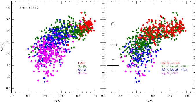
Figure 2: The color locus of star-forming galaxies in optical $B-V$ versus the near-IR $V-3.6$. The left panel divides the S⁴G and SPARC samples by morphological type. The right panel divides the samples by stellar mass, deduced from 3.6$\mu$m luminosity. All morphological types have a range of $B-V$ colors, but spiral differentiate from dwarfs at a $V-3.6$ color of 2.5. Stellar mass is independent of optical color, but is better distinguished by $V-3.6$ color.

The accuracy of the photometry varies based on the original source material (see a similar plot with error bars in Schombert & McGaugh 2014, Figure 6). In general, the error bars increase to bluer $V-3.6$ galaxies as these galaxies are lower in surface brightness as a class (representative errorbars are displayed in Figure 2). The locus of color defined in Figure 2 is larger than the scatter in the observables and reflects a range of age and metallicity paths for the underlying stellar populations (Bell & de Jong 2000). We will use a density map of Figure 2 for comparison to stellar population models in §6.

The right panel in Figure 2 displays the same colors coded by stellar mass (using a value of 0.5 to convert 3.6$\mu$m luminosities into mass, Lelli et al. 2017). The trend for higher masses to be redder follows the well known color-mass and color-magnitude relationships (Tremonti et al. 2004). The trend in color, at first glance, is surprisingly coherent considering that the MSg finds the highest mass star-forming galaxies to have the highest current SFR’s and, presumingly, largest number of young stars. In other words, one might expect that the galaxies with the highest SFR would have the bluest $B-V$ colors. But this naive interpretation ignores the fact that the past SFR must have been much higher in these galaxies and, thus, in high-mass galaxies a majority of the stellar population is composed of old stars with redder colors pushing $B-V$ to redder values (see Figure 4). This can also be seen by the fact that mass is more correlated with $V-3.6$ color than $B-V$, optical colors having a larger range than near-IR colors due to diversity in the SFH and variable internal extinction.

4 Star Formation History

Deducing the star formation history of a galaxy is a convoluted process that attempts to extract the ages of the stars, by number, that make up its stellar population. In practice, this involves extracting the SFR as a function of time and applying a standard initial mass function (IMF) to derive the total luminosity (i.e. stellar mass) for the present epoch. This is the approach used, successfully, by Speagle et al. (2014) by following the main sequence as a function of redshift, effectively measuring SFR as a function of lookback time then piecing together the SFH of a range of galaxies by total mass (see also Leitner 2012).

We can adopt Speagle’s general SFH shape for star-forming galaxies greater than $10^{10}$ $M_{\sun}$ (see their Figure 9). However, the main sequence takes on a different slope for lower mass galaxies suggesting a different form to the SFH for these lower mass systems. Our procedure starts with this general shape and the SFR at the current epoch is the input. This determines the total stellar mass through the MSg. The peak SFR is then normalized such that the integrated stellar mass from this SFH matches the total stellar mass given by the MSg. Figure 3 presents the Speagle et al. SFH, displayed as log SFR with respect to time from galaxy formation ($\tau$). The red curves follow the Speagle et al. shape, normalized such that the final stellar mass agrees with their $z=0$ MSg. Given the shallow slope of the Speagle et al. main sequence, this naturally results in a shaper decline in star formation for higher mass spirals.

The SFH’s for the lower mass end of the main sequence are shown as blue curves in Figure 3. In order to match the main sequence for low-mass galaxies found by McGaugh, Schombert & Lelli (2017), the strength of the initial burst must be lowered with decreasing mass to a larger degree than the high-mass spirals. However, the steeper slope of the MSg, near the line of constant SF, restricts the strength of the initial burst in order to maintain nearly constant SF to the current epoch (needed to match the final total stellar mass to the current SFR). The simplest solution is to extend the duration of the weak initial burst from 4 to 5 Gyrs from galaxies with 10⁹ to 10⁷ $M_{\sun}$. There is some physical choice for this alteration of the SFH with lower mass as it is well known that star formation goes as the density of the gas (i.e., Schmidt’s law). Lower density galaxies naturally have decreased SFR’s; however, higher gas fractions allows for longer durations of SF. In any case, this is simply a numeral choice in order to have the simplest parameters that integrate to the correct total stellar mass given by the Speagle et al. SFH shape, plus end up on the correct position of the main sequence for a given current SFR. This prescription, unsurprisingly, results in a nearly constant, SFR for low-mass galaxies, but also allows for slightly rising or declining SFH (as indicated by the range in $FUV-NUV$ colors) and will be discussed in §6.

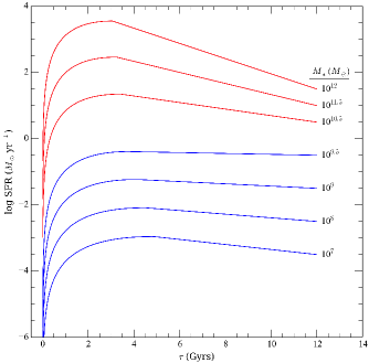
Figure 3: Baseline star formation histories as a function of final SFR. The red curves are for high-mass ($M_{*}>10^{10}M_{\sun}$) galaxies that follow Speagle et al. $z=0$ main sequence. The blue curves are adjusted to match the low-mass main sequence found by McGaugh, Schombert & Lelli (2017). The shallower slope of the Speagle et al. main sequence results in a sharper decline in SFR versus the low-mass systems SFH. These SFH’s form the baseline for comparison in §6, variations on starting epochs, width of the initial burst and rapid changes as also considered.

While the general shape of the Speagle et al. SFH is applied to each mass bin to produce final stellar masses in agreement with the observed main sequence, these SFH’s predict very different integrated properties. This was first explored by Leitner (2012) who uses the Main Sequence Integration technique, combined with high redshift SFR information, to deduce similar SFH’s to Speagle et al. (see his Figure 3) and the mass fraction growth with lookback time. For massive systems, Leitner finds a majority of the stellar mass is in place within 2 to 3 Gyrs after initial SF. However, to maintain the shallow slope of the high-mass MSg, his SFH have later initial SF epochs with decreasing mass. This also has the advantage of slowing the chemical enrichment of low-mass systems, and produce bluer colors as the oldest stars are only 6 Gyrs in age. The steeper slope on the low-mass end of the MSg lowers the current SFR below the extrapolated SFH used by Leitner and forces a longer duration of SF in order to produce sufficient stellar mass.

We can compare the growth in stellar mass given by the fiducial SFH’s in Figure 3. For example, in Figure 4, we can see that the growth in stellar mass and luminosity differs significantly with increasing galaxy mass and the contribution from stars of differing ages also varies significantly with increasing galaxy mass. A low-mass dwarf galaxy achieves 1/2 its total mass by 5 Gyrs from the start of star formation, compared to a high spiral which only takes 3 Gyrs to achieve the same fraction. This results in a higher fraction of older stars for high-mass systems. A slower mass growth rate also reflects into the rate of chemical enrichment, the lower metallicity of LSB galaxies is driven, not only by lower SFR, but by overall slow-mass growth. Based on these results, a different chemical enrichment model will be considered for each mass bin (see §5.1).

Using a standard stellar population model (see §5), the $V$ and $K$ luminosities of a low-mass dwarf reach the midpoint at 7 to 8 Gyrs, whereas a high-mass spiral only requires 4 Gyrs. This explains some of the difference in colors for LSB galaxies versus bright spirals. Despite the higher current SFR rates, most of the stellar mass is locked in stars that are older than 6 to 7 Gyrs, a red population. While most of the stars in an LSB galaxy are younger than 6 Gyrs, their blue colors due to younger mean age, not recent SF. As we will see in §6, growth in optical, compared to near-IR colors, is also weak in high-mass spirals, producing redder $V-K$ colors, versus LSB galaxies which have consistent differences in $V$ and $K$ luminosities resulting in much bluer $V-K$ and $V-3.6$ colors. Thus, the combination of low metallicity, older populations and a stronger contribution from the younger stars is the primary reason that LSB galaxies occupy the bluest colors at all wavelengths, not due to particularly recent formation epochs (Pildis, Schombert & Eder 1997; Schombert & McGaugh 2014).

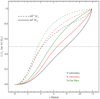
Figure 4: For the baseline SFH in Figure 3, the resulting growth in $V$ and $K$ luminosity plus stellar mass. High mass spirals achieve a 50% line at much earlier epoch’s than low-mass dwarfs, resulting in redder colors. Slow mass build-up also reflects into slow chemical enrichment for dwarfs, plus lower final [Fe/H] values.

Unlike the high-mass end (the land of weary giants, running out of HI), the lower mass end of the main sequence has a more diverse range in recent SFR changes as indicated by their $FUV-NUV$ colors. The line of constant star formation divides the lower mass end of the main sequence plane into two sections; 1) those galaxies where the average past SFR must have been higher than the current SFR (to the right of the constant SFR line) and 2) those galaxies where the average past SFR must have been lower than the current SFR (to the left of the constant SFR line). All galaxies higher in mass than $10^{10}$ $M_{\sun}$ lie to the right of the constant SFR line and, thus, have declining SFRs in agreement with the deduced SFH from Speagle et al. (2014). However, the low-mass sample divides neatly by $FUV-NUV$ around the constant SFR line (shown as red and blue symbols in Figure 1).

As shown by Murphy et al. (2011), dust-corrected $FUV$ luminosity is a proxy for the current SFR rate on timescales of a few 100 Myrs (in contrast, H$\alpha$ luminosity measures a shorter timescale, around 20 Myrs). The mean $FUV-NUV$ color for star-forming galaxies is 0.25 with a standard deviation of 0.10. However, dividing the sample by $FUV-NUV=0.25$ displays a surprising dichotomy in Figure 1. There are 187 galaxies with $FUV-NUV$ colors. Of the $GALEX$ sample, 87 have $FUV-NUV<$ 0.25, 100 are redder. Of the blue sample, 57 are to the right of the constant SFR line (67%), versus 25 of the red sample (25%). Thus, a majority of star-forming galaxies with blue $FUV-NUV$ colors lie to the left of the constant SFR line indicating that those galaxies have rising SFR’s over that last few 100 Myrs. Likewise, star-forming galaxies with red $FUV-NUV$ colors have declining SFR’s over the same timescale and lie to the right of the constant SFR line. No correlation between $FUV-NUV$ and $B-V$ is found, indicating that changes in SFR occur on timescales of 100 Myrs, but are stable over Gyr timescales. This is in agreement with the deduced SFR over the last Gyrs in the WFC3 CMDs for three LSB galaxies (Schombert & McGaugh 2015).

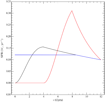
Figure 5: Three possible SFH scenarios that reproduce the low-mass end of the main sequence. The black line displays the baseline SFH from Speagle et al. , normalized such that the current SFR matches the total stellar mass produced by the integrated SFH. The red line is a late formation scenario, where initial star formation is delayed by 4 Gyrs. The initial burst must be increased to produce the expected stellar mass. The blue line is a scenario where the initial burst is extended by several Gyrs, resulting in a lower peak burst.

The above dichotomy in $FUV-NUV$ colors indicates that the last stages in SFH scenarios for low-mass dwarfs are sensitive to upward and downward changes in SFR. The sample from LSB+SPARC straddle the constant SFR line, although a majority lie on the right hand side indicating a declining SFR. As the $FUV-NUV$ color correlates with position with respect to the constant SFR line, we consider two avenues for the SFH lower mass galaxies, one with a declining SFR of the last Gyr to its current value, the second with a rising SFR over the last Gyr. However, even with this constraint, there are numerous potential SFH’s that achieve the observed trend of stellar mass with current SFR such that they 1) have the correct final mass for the final SFR, 2) have recent SFR that are either greater than or less than the current rate (depending on $FUV-NUV$ color) and 3) are declining or rising over the last Gyr (again, defined by current $FUV-NUV$ color). For example, Figure 5 displays three possible scenarios that satisfy the above conditions for those low-mass galaxies with declining SFR. Each, scaled to the appropriate initial burst, can reproduce the observed low-mass main sequence, but predict very different final colors (see §6).

In addition, we consider the effects of episodic star formation, particularly in recent epochs (Noeske et al. 2007; Haywood et al. 2018). In this scenario, we alter the SFH’s in Figure 5 with sharp changes in SFR over the last Gyr. These small bursts must be fairly constrained otherwise there would not be a strong correlation between $FUV-NUV$ and optical colors, such as $B-V$. The scatter in the $B-V$ versus $FUV-NUV$ diagram is 0.13 dex, where most of the uncertainty is due to observational error on the colors. A conservative estimate is that the SFR for galaxies with $B-V<0.7$ has not deviated more that 15% in the last couple Gyrs (the timescale sampled by $B-V$). Similar estimates are obtained from comparison with $U-B$ and $U-V$ colors.

The main sequence will not constrain any of the above scenarios. However, each does make specific predictions on the final integrated colors of galaxies. Thus, additional constraints can be obtained by using spectral energy distribution (SED) models (Bruzual & Charlot 2003; Conroy & Gunn 2010) to predict present-day colors from a given SFH history, then comparing this to the color locus of star-forming galaxies binned by total stellar mass. The input parameters (such as age and metallicity distribution) are the critical unknowns in producing a reliable color locus for star-forming galaxies. Fortunately, new observations from $GALEX$ to $Spitzer$ combined with HST CMD’s of nearby LSB galaxies (Schombert & McGaugh 2015) serve to guide those inputs.

For the sake of numerical experiments in §6, we divide the low-mass SFH scenarios into five classes; 1) baseline (following the prescription deduced by Speagle et al. ), 2) late (a formation epoch delayed by 4 to 5 Gyrs), 3) wide (an extended initial burst of lesser intensity), 4) rising (a lower initial burst with a slightly rising SFH) and 5) episodic (varying the late stages of SF by 20%). Each scenario is mapped onto the main sequence as a boundary condition to the total level of star formation (shown in Figure 5) with some adjustment to consider rising or declining star formation based on the division by $FUV-NUV$ color. Each scenario can then be mapped into a stellar population plus chemical enrichment model, as discussed in the next section.

5 Stellar Population Models

A previous paper by the SPARC team (Schombert & McGaugh 2014) derived the $\Upsilon_{*}$ ratio of star-forming LSB galaxies based on experience with elliptical colors and the SED models from Bruzual & Charlot (2003, hereafter BC03). In that paper, empirical color relationships were used to extended the behavior of the BC03 models to farther wavelength’s, particularly the $Spitzer$ 3.6$\mu$m filter and also considered the effects of AGB, BHB and lower metallicity stars on the integrated colors in a semi-empirically fashion. While that technique was sufficient to derive $\Upsilon_{*}$ for simple star formation histories, the more complicated paths outlined in §4 require a more sophisticated treatment. Thus, we turn to the SED models produced by Conroy & Gunn (2010, hereafter CG10) which allow more flexibility in the contribution of exotic populations (such as AGB and BHB stars) than the BC03 models, and offer colors from $GALEX$ to $Spitzer$. For standard stellar populations assumptions (i.e., the same IMF and isochrones) both BC03 and CG10 agree on both optical and near-IR colors, demonstrating consistence in their techniques.

Our procedure is similar to that outlined in Schombert & McGaugh (2014), each model is the sum of a number of simple stellar populations (SSPs) which consists of a unit mass of stars of the same age and metallicity. Each SSP is initialized with a selected IMF and each stellar mass bin has been evolved to a set age using a suite of stellar isochrones (see CG10 or BC03 for details of the stellar libraries). At any particular age, the sum of all the previous SSP’s (we use timesteps of 0.01 Gyrs) weighted by the luminosity of the stellar population is output either as a single spectra, or convolved through a set of standard filters. By integrating their entire spectrum of each SSP we can achieve a goal, as noted by Roediger & Courteau (2015), that increasing wavelength coverage significantly reduces the uncertainty and systematic errors in $\Upsilon_{*}$ and, thereby, stellar mass estimates. The scripts to perform these calculations are available at our website.

While the evolution of a stellar population using isochrones is a stable calculation, there are numerous subtleties to the detailed calculations. For example, the IMF used to make the initial mass distribution can vary (e.g., a Salpeter 1955, Kroupa 2001 or Chabrier 2003 style). Metallicity is straight forward, but variations of the $\alpha$ element ratio (typically expressed as $\alpha$/Fe), driven by the time sensitive ratio of Type Ia to Type II SN, effects the number of free electrons in a stellar atmosphere, which in turns alters the temperature of the RGB. The contribution of blue horizontal stars (BHB) and blue stragglers (BSs) is a free parameter as is the treatment of thermal pulsing asymptotic giant branch (TP-AGB) stars. The former being important for optical colors, the later dominating the near-IR colors.

Globally, the relevant inputs are the star formation history plus a chemical enrichment model. These allow each individual SSP to be summed over the SFH with each SSP using the [Fe/H] value at each epoch as given by the enrichment model. The check on the final result will be the models position on the main sequence (stellar mass versus current SFR), reproducing the mass-metallicity relation (the stellar mass versus average [Fe/H] value for the model), the internal metallicity distribution (compared to the MW, e.g., the G dwarf problem) and the integrated model colors. All the details of gas infall, recycling and stellar remnants are contained in the chemical enrichment models, so this will be discussed first.

5.1 Chemical Enrichment Model

The basic assumption behind a basic chemical evolution scenario is instantaneous recycling of enriched material by mass loss or supernovae ejecta (Pagel 1997). While it does take a finite amount of time to process the ISM through the birth and death of stars, fortunately, for the calculations, the recycling timescales are much shorter than the timesteps used for our SFH models (Matteucci 2007). The one exception to this rule is the effect of the $\alpha$/Fe ratio which can require Gyrs to build-up and will be discussed in §5.2.

For the galaxies we attempt to model, we are guided by the age-metallicity scenarios proposed by Prantzos (2009) based on an analysis of the stars in the Milky Way. The scenario has several common features with observations of MW stellar populations; 1) a pre-enriched population with [Fe/H] $=-1.5$, 2) a rapid rise to approximately 80% of the final metallicity in 5 Gyrs, then 3) a slow rise to the final [Fe/H] of the current epoch. A small adjustment to the model is made to account for the lower percentage of metal-poor stars than predicted by the models (i.e., the G-dwarf problem, see Schombert & Rakos 2009).

Initial comparison between the models and CMD diagrams of nearby galaxies suggests that the Prantzos scenario for the MW over-estimates the rise in metallicity for low-mass galaxies and under-estimates the enrichment rate for high-mass galaxies. To produce a more realistic model, we alter the form of the Prantzos scenario into three types; slow, normal and fast. The slow version is basically a linear increase in [Fe/H] with age, simulating a LSB dwarf with very slow SFRs. The fast version is a slightly more rapid rise (reaching 80% final metallicity in 2 Gyrs, rather than 5 to simulate a strong initial burst, as expected for high-mass, high SFR spirals. Given that we know, due to the steep slope of the main sequence below $10^{10}$ $M_{\sun}$, that low-mass, LSB galaxies have either slowly rising or slowly declining SFH’s, a slower chemical enrichment seems appropriate. We adopt the normal Prantzos scheme for MW sized spirals, and the faster scheme for high-mass spirals, again based on the slope of the main sequence.

As an external check to the merit of our enrichment prescriptions, we examined the internal metallicity distribution functions (MDF) of the final stellar populations and compared these to observed MDF’s in ellipticals, spirals and the Milky Way (Haywood et al. 2018). We found that the shape of the MDF’s were similar to the MW MDF (including the G dwarf deficiency) and, as demonstrated in Schombert & Rakos (2009), the importance of low metallicity stars decreases with lower mean metallicities as the MDF’s compress in metallicity range. For [Fe/H] values below $-$0.5 (approximately 10⁹ $M_{\sun}$ on the main sequence) the shape of the MDF was irrelevant to the colors of the integrated stellar population.

Lastly, we need to assign a final [Fe/H] to each enrichment model. We are guided by the various mass-metallicity relation studies using O/H values for star-forming galaxies (see Tremonti et al. 2004, Zahid et al. 2011 and Brown et al. 2018) First, the relationships from these studies can be extrapolated to stellar masses between $10^{8}$ and $10^{11}$. We convert the deduced O/H values into [Fe/H] using the prescription from McGaugh (1991). Second, for stellar masses below $10^{8}$ $M_{\sun}$, we use the [Fe/H] values which have been measured directly for three LSB dwarfs (see Schombert & McGaugh 2015). These dwarfs, with stellar masses around $10^{7}$ $M_{\sun}$, have [Fe/H] values between $-$1.0 and $-$0.6 with a mean value of $-$0.7 at stellar masses of 10⁷ $M_{\sun}$. Thus, we assume a [Fe/H] value of $-$1.2 for our lowest mass galaxies, rising to a value of $-$0.5 where O/H values are available around stellar masses of $10^{8.5}$ $M_{\sun}$.

5.2 $\alpha$/Fe Corrections

The colors of stellar populations are determined by the distribution of stars, given by stellar isochrones, in the HR diagram. Decreases in metallicity drive both the turnoff point and the position of the RGB to hotter temperatures, i.e. bluer colors, due to changes in line blanketing and opacity. While Fe is the main contributor of electrons to produce color changes, all atoms heavier than He can contribute electrons. It is typically assumed that all the elements track Fe abundance, but it is possible to have overabundances of various light nuclei (so-called $\alpha$ elements) under certain conditions.

The $\alpha$ elements, everything lighter than Fe, are primarily produced in massive stars (Type II SN), while a higher contribution to Fe comes from Type Ia SN. Since SNII are short-lived ($\tau<10$ Myrs) and SNIa detonate only after a Gyr (the average time for the white dwarf to form), the ratio of $\alpha$/Fe measures these different formation timescales. At early epochs, for a stellar population undergoing constant SF, the ratio of $\alpha$/Fe is high as determined by Type II supernovae. Then, after a Gyr, the $\alpha$/Fe ratio begins to decrease due to the contribution of products from SNIa explosions (c.f., McWilliam 1997, and references therein).

For example, in elliptical galaxies the ratio of $\alpha$/Fe is a factor of four higher than metal-rich stars in the Milky Way due to the short timescales of initial, very strong bursts star formation (Thomas et al. 2004). As star formation is extended in star-forming disks and irregulars, those galaxy types have lower $\alpha$/Fe ratios as more recent star formation is enriched in Fe from Type Ia SN (Matteucci 2007). For a constant star formation scenario, we can model the ratio of $\alpha$/Fe as a function of [Fe/H] following data from the Milky Way (Milone, Sansom & Sanchez-Blazquez 2010) with [Fe/H] serving as a proxy for age. In their data, elliptical-like $\alpha$/Fe ratios are found up to $[Fe/H]=-1.0$, then drops quickly to a solar value at solar metallicities. We can apply the same behavior to our models.

The effect of the $\alpha$/Fe ratio on colors was outlined in Cassisi et al. (2004). With respect to colors, $B-V$ decreases (bluer) with increasing $\alpha/Fe$, for example a metal-poor population ([Fe/H]=$-$1.3) had a $B-V$ shift of $-$0.03 for an increase in $\alpha$/Fe by a factor of four. A solar metallicity population is shifted by $-$0.07 blueward for the same change in $\alpha$/Fe. Similar shifts are expected in $V-K$ with $\Delta(V-K)$ ranging from $-$0.06 for metal-poor populations to $-$0.09 at solar metallicity.

To incorporate these corrections into our models, we assume that $\alpha$/Fe decreases, in a linear fashion (as Fe increases from Type Ia SN events), from an initial value of 0.4 to a solar value (0.0) over one Gyr of time starting two Gyrs after initial star formation. This mimics the behavior seen in ellipticals and, thus, only the first three Gyrs of star formation have differing $\alpha$/Fe values from solar. For star-forming galaxies less that $10^{9}$ $M_{\sun}$, the assumed chemical enrichment scenario is much slower than what we used in Schombert & McGaugh (2014). This would serve to decrease the impact of an $\alpha$/Fe correction as most of the stars with high $\alpha$/Fe ratios are still quite low in metallicity (typically below [Fe/H] $=-1.0$). For slowing rising or slowing declining SFR, less than 25% of the total stellar population requires an $\alpha$/Fe correction. Our initial experiments indicated that this correction is very small and we will only consider this correction in the color error budget (see §6).

5.3 Dust

For this study, we follow the phenomenological dust models used by Conroy & Gunn (2009). Dust affects galaxy colors through three avenues; 1) dust specific to young stars (remnants of the stellar nursery), 2) circumstellar dust associated with AGB stars, and 3) general dust attenuation from the diffuse ISM, which reddens integrated colors with decreasing strength to longer wavelengths. Dust attenuation for young stars arises due to the dust in the molecular clouds in which very young stars are embedded. The timescale for this attenuation is $10^{7}$ years (Charlot & Fall 2000) and only applies to the last timestep of our models. In addition, at log SFR $<-2$, the luminosity from young stars makes this correction negligible. Circumstellar dust around AGB stars can play a significant role in the colors of that short-lived population. It is a metallicity dependent factor, but can be tested for in our models by comparison of near-IR colors of LMC/SMC young clusters (see §6).

General dust attenuation, generated by the diffuse ISM, is best handled using a phenomenological model that is not computationally expensive (Conroy, White & Gunn 2010). In this case, an SSP of a set age has an attenuation curve with a age dependent shape and normalization. As the grain properties of dust are dependent on mean metallicity (Guiderdoni & Rocca-Volmerange 1987), the effects of attenuation also decreases with lower [Fe/H] for the stellar population (assumed to be one of the reasons low metallicity LSB galaxies have never been found to have dust features nor far-IR emission). Also, unlike extinction due to dust in the Milky Way, dust in external galaxies scatters blue light which, on average, reenters the line-of-sight (Calzetti 2001). This works to minimize any corrections for dust, however, again, we will note this effect in our error budget and find the corrections for the low-mass end of the MSg to be negligible.

5.4 BSs and BHB Populations

Two exotic stellar populations can play an important role for optical colors, blue horizontal branch (BHB) stars and blue straggler stars (BSs). Horizontal branch stars are old, low-mass ($M<1M_{\sun}$) stars which have entered the helium core burning phase of their lives. They are bright ($M_{V}=-5$), of nearly constant luminosity and range in color from red to blue (RHB and BHB stars). BHB stars are of interest to galaxy population models for they have similar characteristics to young stars in color parameter space, although they are not a signature of recent star formation.

Blue stragglers stars (BSs) occupy a position in the HR diagram that is slightly bluer and more luminous than the stellar populations main sequence turnoff point (Sarajedini 2007). Their extended main sequence lifetime appears to be due to binary mass exchange, either by close contact binaries (McCrea 1964) or direct collision (Bailyn 1995). Their importance to stellar population synthesis is that they occupy a region of the HR diagram that mimics star formation and low metallicity effects (i.e., increased contribution to the blue portion of the integrated SED).

The effect BHB stars on population models is limited in time and metallicity. BHB stars are primarily found in metal-poor clusters ($[Fe/H]<-1.4$) and are not found in any population younger than 5 Gyrs. Very few BHB stars are found in the solar neighborhood (Jimenez et al. 1998), presumingly a combination of young age and high metallicity, so their contribution in field populations is unclear. Considering low-mass galaxies with a slow chemical evolution then, at the start of a constant star formation scenario, 50% of the stellar population has the metallicity and age appropriate for a BHB phase. Following the prescription of Conroy, Gunn & White (2009), this corresponds to a $f_{BHB}=0.5$ which translates into a $\Delta(B-V)$ of $-$0.05 and a $\Delta(V-K)$ of $-$0.03 for a low metallicity SSP ($[Fe/H]<-1.0$). For a SFH dominated by a strong initial burst, this factor would be slightly larger (up to 60% of the final stellar population). For a rising SFH, this effect will be smaller (down to 25%).

With respect to the BSs population, a more general problem of binary star evolution is outlined in Li & Han (2008) which takes into account binary interactions such as mass transfer, mass accretion, common-envelope evolution, collisions, supernova kicks, angular momentum loss mechanism, and tidal interactions (Hurley, Tout & Pols 2002). The results from those simulations indicate that, while BSs’s are difficult to model and relatively time sensitive, they are similar to BHB stars in that they only contribute after a well-formed turnoff point develops at 5 Gyrs. If collisions are important for their development, then they will be more rare in galaxy stellar populations due to lower stellar densities compared to globular clusters. They appear to be numerous in the Milky Way field populations (Preston & Sneden 2000), but are an order of magnitude less luminous than BHB stars.

The simulations of Li & Han (2008) display a maximum of $-$0.03 bluer colors in $B-V$ and $-$0.10 bluer colors in $V-K$ for populations older than 5 Gyrs. The spread in metallicity is small for $B-V$, approximately 0.01 and non-existent for $V-K$. Again, following the prescription of Conroy, Gunn & White (2009), the same level of significance for BSs as for BHB stars results in only a $\Delta(B-V)$ of $-$0.02 and a negligible effect on $V-K$. This is mostly due to the lower luminosity of BSs populations.

For older populations, it appears that BHB stars dominate in luminosity over BSs stars simply based on the fact that BHB corrections to SSP and elliptical narrow band colors are sufficient to reproduce the color-magnitude relation (Schombert & Rakos 2009). For the scenario of constant star formation, by the age where BHB stars decrease in their contribution ($\tau<5$ Gyrs), BSs stars would be beginning to influence the bluest wavelengths. However, young stars quickly overwhelm the BSs luminosities and our simulations indicate that the BSs contribution is negligible when compare to other factors.

5.5 TP-AGB Treatment

An important component for the near-IR colors is the treatment of thermally-pulsating AGB stars (TP-AGBs or just AGB). These are stars in the very late stages of their evolution powered by a helium burning shell which is highly unstable. They are stars with high initial masses ($M>5M_{\sun}$) and intermediate in age ($\tau>10^{8}$ years). While the BC03 codes (and their extension, see Bruzual 2009) include AGBs as part of their evolutionary sequence, comparison with other codes (e.g., Maraston 2005, Gonzalez-Perez et al. 2014) finds discrepancies in the amount of luminosity from this short lived population.

The history of AGB treatment in SED codes is outlined in CG10. To determine which model best fits our AGB prescription, we compare the extension of BC03 and CG10 to the near-IR colors of LMC and SMC star clusters (see Figure 6). As metallicity typically decreases for older star clusters, it is problematic to compare a single metallicity SSP track to the colors versus age in Figure 6. However, as can be seen in Figure 6, a solar metallicity model accurately captures the young cluster colors. There is very little difference between the solar BC03 and CG10 tracks, although adding a standard AGB dust model (Villaume et al. 2015) compares more favorably with the redder young cluster colors. The variation in metallicity is only important for very young and very old clusters.

As noted in Schombert (2016) and Schombert & McGaugh (2014), all the models were poor matches to the near-IR colors of populations older than a few Gyrs. We will still consider an empirical enhancement to model $V-K$ and $V-3.6$ colors for old, metal-poor components. However, comparison between metal-poor ([Fe/H] $<-1.0$) and metal-rich ([Fe/H] $>-1.0$) MW globulars (magenta points in Figure 6) finds that the CG10 and BC03 models accurately predict their $V-K$ colors. The discrepancy between model and observations occurs, primarily, for the clusters with ages near $10^{9}$ yrs.

In a recent development, any corrections from our original paper (Schombert & McGaugh 2014) are now drawn into question. Not due to changes in SED models, but rather the recent HST observations on three, nearby LSB dwarfs (Schombert & McGaugh 2015). The F555W-F814W CMD’s for LSB galaxies F415-3, F608-1 and F750-V1 display a dramatic lack of AGB stars (only 5 to 10% compared to 20% for other metal-poor, high SFR dwarfs). A lack of AGB stars was doubly surprising as the metallicities of these LSB dwarfs ([Fe/H $\approx$ $-0.8$) was in the realm where AGB stars have a stronger contribution than for higher metallicity dwarfs. It appears that the extremely low past SFR for LSB galaxies (log SFR $<-3$) combined with the short lifetimes for the AGB population under produces, by a significant fraction, the expected numbers from simple SFH scenarios.

To account for this deficiency, we use the CG10 models ability to alter the contribution from AGB stars, and allow for an underabundance, or overabundance, to be considered combined with a metallicity threshold. Thus, we consider two AGB corrections, one where the AGB component is suppressed, as indicated for low-mass dwarfs from WFC3 observations, and a second scenario where the near-IR luminosities are slightly boosted between 0.1 and 2 Gyrs in concurrence with LMC/SMC cluster observations (Ko, Lee & Lim 2013).

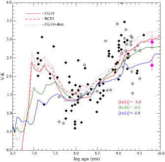
Figure 6: $V-K$ colors of LMC/SMC star clusters from Kyeong et al. (2003, solid symbols) and Pessev et al. (2006, open symbols). Averages for [Fe/H] $<-1.0$ and $>-1.0$ MW globulars from Cohen et al. (2007) are shown as magenta symbols. The red lines are solar metallicity SSP’s from BC03 and CG10, with and without dust as indicated. The solar metallicity models are a good match to the young clusters, but a poor match to the metal-poor older clusters. Lower metallicity SSP’s (green and blue) reproduce the intermediate age clusters, but also fail to match the redder colors of the oldest clusters.

5.6 Empirical Calibration of Near-IR Colors

The SPARC dataset depends on $Spitzer$ 3.6$\mu$m observations to determine the stellar mass which, when combined with the gas mass, becomes the total baryon mass of a galaxy. An accurate $\Upsilon_{*}$ requires a valid stellar population model at the $Spitzer$ wavelengths, however, the BC03 models do not extend beyond $K$ (3.2$/mu$m). To correct for this, Schombert & McGaugh (2014) used an empirical $K-3.6$ calibration, based on $2MASS$, $WISE$ and $Spitzer$ observations, to convert BC03 $\Upsilon_{*}^{K}$’s into $\Upsilon_{*}^{3.6}$. In the interim, improved $K$ observations and additional $Spitzer$ observations have been obtained for the SPARC sample. When combined with existing datasets, such as S⁴G (Sheth et al. 2010), this allows for a detailed comparison with the CG10 models, which use an extended stellar library to offer 3.6$\mu$m colors, and near-IR colros. Figure 7 displays the two color diagram for $B-V$ versus $K-3.6$ using the SPARC plus S⁴G samples. A least-squares fit is shown ($K-3.6=-0.42\pm 0.02(B-V)+0.54\pm 0.01$) and symbol type divides the sample into high and low-mass systems (divided at $10^{10.5}$). As found by Schombert & McGaugh (2014), the mean $K-3.6$ color is around 0.3 with a slight color term such that optical bluer galaxies have slightly redder $K-3.6$ colors.

Also shown in Figure 7 are the SSP tracks from CG10, each track displaying colors for ages greater than 0.5 Gyrs. The general trend of the SSP tracks is the same as the fitted linear slope. Higher metallicity models have redder $K-3.6$ colors at a set $B-V$ color, and this effect can been seen in the sense that high-mass galaxies lie above the linear fit, as expected for their higher metallicities. But, there is significant scatter in this trend. For example, the 10 Gyrs models for varying [Fe/H] are, basically, a line of constant $K-3.6$ color of a value of 0.14. This minimizes its usefulness as a metallicity indicator, but supports the expectation that $\Upsilon_{*}$ deduced from 3.6$\mu$m colors will be the most stable under varying age and metallicity conditions and confirms the CG10 tracks.

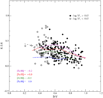
Figure 7: The two color diagram for $B-V$ versus $K-3.6$ using the SPARC plus S⁴G samples. A least-squares fit is shown and symbol type divides the sample into high and low-mass systems (divided at $10^{10.5}$). As found by Schombert & McGaugh (2014), the mean $K-3.6$ color is around 0.3 with a slight color term such that optical bluer galaxies have slightly redder $K-3.6$ colors. Also shown are four SSP models from CG10 for [Fe/H] values of +0.2, 0.0, $-$0.5 and $-$1.0 (more metal-rich have redder $K-3.6$ colors). The SSP’s range from $10^{8}$ to $10^{10}$ years in age.

6 Discussion

6.1 Effects of Varying Stellar Population Parameters

For our simulations, we consider a range of SFH’s and mixtures of exotic stellar population components, particularly for the low-mass end, using the Speagle et al. shape as a baseline. We consider log SFR_o = 0.0 as the crossover point from the lower to upper main sequence, and the point where the strength of the initial SF burst alters to produce higher mass spirals. Table 1 displays our baseline stellar population parameters based on the MSg and the mass-metallicity relation. At each log SFR_o (the current SFR from the MSg), we assign a final metallicity (where all the simulations begin with a initial [Fe/H] value of $-$1.5). For the high-mass end, we map log SFR_o into final [Fe/H] values of $-$0.2, +0.1 and +0.2 for total stellar masses of $10^{9.5}$, $10^{10.5}$ and $10^{11.5}$ $M_{\sun}$ respectfully. On the low-mass end, we adopt final [Fe/H] values of $-$1.2, $-$0.7 and $-$0.4 at log SFR_o = $-$3.5, $-$2.5 and $-$1.5 respectfully.

In addition to final metallicities, we also adopt a chemical enrichment model that best represents the total stellar mass, gas fraction and predicted SFH. For low-mass, LSB-type dwarfs, with high gas fractions and low SFR over their SF histories, we assume a slow evolution in metallicity, we adopt a linear growth in [Fe/H] with time. For galaxies near 10¹⁰ $M_{\sun}$, we adopt the Prantzos (2009) prescription. For the high-mass end, with high initial SFR’s, we assume a faster chemical enrichment and adopt a fast form of the Prantzos (2009) prescription, where the 80% final enrichment is reaching in only a few Gyrs.

Table 1: Baseline SFH parameters

log SFRoa	log $M_{*}$b	[Fe/H]oc	[Fe/H]d
($M_{\sun}$ yr-1)	($M_{\sun}$)		rate
$-$3.5	107	$-$1.2	slow
$-$2.5	108	$-$0.7	slow
$-$1.5	109	$-$0.4	slow
$-$0.5	109.5	$-$0.2	normal
+0.5	1010.5	+0.1	fast
+1.0	1011.5	+0.2	fast

• the current star formation rate

• total stellar mass

• final mean metallicity

• chemical evolution rate

The conditions outlined in Table 1 represent the baseline SFH plus chemical evolution that fits the observations for both the high and low-mass ends of the main sequence. We will alter then shape of the SFH (always to produce the correct slopes of the MSg), as outlined in §4, but not the chemical evolution scenarios. We will also indicate the effect of changing mean [Fe/H] in the following two color diagrams, but maintain the same chemical enrichment for two reasons. First, for the low-mass end, the final metallicities are already very low and the change in the chemical growth (and resulting metallicity distributions) are negligible at these low values. On the high-mass end, the rapidity of chemical enrichment under high SFR build-up results in internal metallicity distribution that are dominated by high metallicity stars. Thus, we found that changes in the style of chemical enrichment was negligible on the final galaxy colors.

The color results for the baseline models, listed in Table 1, are shown in Figure 8. The baseline model is shown as a magenta zone, using the Speagle et al. SFH, which the width of the zone represents varying the baseline model by 2$\sigma$ in metallicity from the mass-metallicity relation (this differs from varying the metallicity of the stellar population, see below). The blue line is the BHB+BSs enhanced model, where the fraction of BHB and blue stragglers are enhanced in agreement with the results from the CMD of LSB dwarfs (Schombert & McGaugh 2015). The red line represents the AGB suppressed model, also in agreement with LSB CMD’s. The dashed line displays the effects of adding an elliptical-like bulge to a solar metallicity star forming disk in varying bulge to disk ratios (i.e., recovering large bulge, early-type spirals). The CG10 SSP for a [Fe/H] = $-$2 is also shown to represent the very minimal metallicity acceptable for galaxy populations. The various error budget vectors are also indicated in the bottom right of the panel and discussed below.

In general, the baseline model works well for high-mass spirals, unsurprisingly as those galaxies on the high-mass end of the main sequence that are well mapped into the Speagle et al. SFH. For lower mass galaxies (with bluer colors) the color locus is consistently too blue in $B-V$, or too red in $V-3.6$, compared to the baseline models. Increasing the AGB contribution serves to redden the $V-3.6$ color by the correct amount, but is in tension with decreasing contribution by AGB’s found for low metallicity LSB dwarfs. This shift would also make the very blue optical colors for a majority of low-mass galaxies difficult to reconcile with redder $V-3.6$. An increasing blue component (BHB+BSs) is agreement with CMD diagrams of nearby dwarfs (see Schombert & McGaugh 2014) and matches the color locus in the sense that the low metallicity models match the low ($B-V<0.4$) colors of many LSB dwarfs. Perhaps the most realistic model is a blend of BHB+BSs enhance and AGB deficient models for LSB dwarfs.

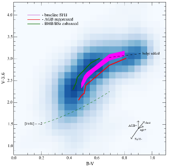
Figure 8: The two color diagram from Figure 2 drawn as a Hess diagram where the photometric errors are used to normalize a 12x12 grid. The baseline SFH from Speagle et al. is shown as the magenta zone (see Table 1 for the midline values). The AGB suppressed model is shown in red, the BHB+BSs enhanced model is shown in green. Various error budget arrows are shown for changing dust, age, metallicity and AGB component. The dashed green line represents the lowest available metallicity SSP model for [Fe/H]=$-$2. The dashed black line represents the effect of a solar metallicity disk with an increasing bulge component from 0 to 100% to mimic the color changes due to the morphology of early-type spirals (Sb to S0). In general, the baseline scenarios match the colors of high-mass star-forming galaxies, but fail to match the low-mass galaxies by often being too red in optical colors and too blue in near-IR colors.

Our first test was to compare the effect on colors to changing forms of the IMF. Comparison between the Salpeter, Chabrier and Kroupa IMF formulations was made for models with [Fe/H] = $-$0.5 and solar. The lower the metallicity, the lower the differences in optical colors. For example, the [Fe/H]=$-$0.5 model resulted in mean differences of 0.001 in $B-V$. In the near-IR, the differences were slightly higher, at 0.005 in $V-3.6$, while relatively constant with metallicity. From this simple experiment, we conclude that IMF changes of these quantities were negligible with respect to color, but may be significant for $\Upsilon_{*}$ calculations (see §7).

Next, we investigated the effects of dust on the baseline models. We use the standard dust model from Conroy, White & Gunn (2010), but ignore the circumstellar dust associated with AGB’s. We ignore AGB dust primarily because the baseline models accurately predict the $V-K$ colors of LMC/SMC clusters without additional dust contributions. Any dust contamination in those clusters appears minimal, so corrections would be inappropriate. The error for dust in $B-V$ versus $V-3.6$ is shown in Figure 8. While it has a slight metallicity dependence, the variation is less than 20%, and the uncertainty arrow in Figure 8 is a median value. Given the global dust abundance as a function of morphological type, we expect dust to have a negligible effect on optical colors in the bluest galaxies due to the lack of far-IR emission in those galaxy types.

Given that the baseline models fit the high-mass end of spiral colors well, the addition of dust (dominant at those morphological types) seems excessive. We note that we do correct our colors for internal extinction using the RC3 prescriptions based on inclination. This appears to mitigate any model dependent dust effects. For the purposes of calculating $\Upsilon_{*}$ from the stellar population models, we have ignored any additional corrections for dust other than standard corrections for internal extinction (Sandage & Tammann 1981).

The largest dependence in color space is, of course, metallicity. Mostly through the temperature of the RGB, but also significantly with respect to line blanketing in the UV to blue portion of the spectrum. While each of the model tracks in Figure 8 accounts for variations in mean metallicity, and a chemical enrichment model to produce an internal MDF, a inaccurate final assumed [Fe/H] value will result in erroneous colors. The error vector in Figure 8 displays the change in color for an error of 0.5 dex in the final [Fe/H] (a fairly extreme value). Note that variable [Fe/H] follows the same basic slope as the color locus, thus, the scatter in the two color diagram is not, primarily, from variations in mean [Fe/H].

Age reflects into the error budget primarily in some error with respect to the formation epoch. A later formation time naturally produces bluer colors as the mean age decreases. While this will be addressed specifically below, by varying the SFH model, a rough estimate of the effect of increasing age is shown in Figure 8 for a change of 2 Gyrs in mean age. This also roughly displays the effect of a "frosting" model (Trager et al. 2000) where a younger stellar population is arbitrarily added to a SFH model, perhaps simulating the merger of a younger system. In either case, the effects of age in the two color diagram are less than metallicity, but notable.

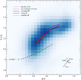
Figure 9: Shown are the SFH models from Figure 5. The baseline model from Table 1 is shown as the dotted line. A scenario where initial star formation is delayed by 4 Gyrs is shown as the magenta line. A scenario where the initial star formation burst is extended in time is shown as the red line. A scenario where is rising over the last 2 Gyrs (rather than declining as in the baseline scenario) is shown as the blue line. Lastly, an episodic scenario where the SFR varies by 50% over the last 2 Gyrs is shown as the green line.

6.2 Effects of Varying Star Formation History

Figure 9 displays the changes in the two color diagram for changes in the SFH from Figure 5. The baseline model from Table 1 is shown as the dotted line. A scenario where initial star formation is delayed by 4 Gyrs is shown as the magenta line. A scenario where the initial star formation burst is extended in time is shown as the red line. A scenario where the SFR is rising over the last 2 Gyrs (rather than declining as in the baseline scenario) is shown as the blue line. Lastly, an episodic scenario where the SFR varies by 50% over the last 2 Gyrs is shown as the green line.

As can be seen in Figure 9, changes in the details of the SFH scenario have only a minor effect on the colors. The only significant change is noted by the late SF model, which mostly extends the near-IR colors to redder colors at higher rates of SF in recent epochs. Aside from the late SF scenario, all the other scenarios match the high-mass side colors.

On the low-mass side, the difficulty with all the models is reaching the blue optical colors representative of LSB galaxies. While many of the scenarios can reproduce the redder near-IR colors at a particular $B-V$, none of the SFH scenarios adequately match the colors of the blue end of every two color diagram. Given that nearly half of the low-mass galaxies in the Cook et al. and LSB+SPARC samples have blue UV colors, this would seem to support a rising SF scenario for a significant fraction of the low-mass galaxies. However, an additional blue stellar component is required even for the rising SF scenario.

In summary, the baseline SFH scenario, outlined in Table 1, recovers the general characteristics of the color locus from Figure 2 on the high-mass side, but predicts much redder optical colors than observed on the low-mass side. The addition of a bulge component improves the color predictions on the high-mass side to recover the effect of large bulges on early-type spirals. However, the baseline scenario does not reach the blue colors of low-mass dwarfs and LSB galaxies, which requires some additional blue component in the optical, without a significantly increasing in near-IR colors.

A hot component such as BHB and BSs stars satisfies this criteria and agrees with CMD results from nearby galaxies. A rising SF in the last few Gyrs will also reach this region of the two color diagrams, but a substantial rise in SF will not reproduce the slope of the MSg (i.e., the rising SF models do not smoothly connect with the high-mass end of the MSg). A deficiency in AGB stars is difficult to explain in the two color diagrams, and the deficiency found by Schombert & McGaugh (2014) will need to be confirmed with near-IR CMD’s.

The SFH scenarios can now be mapped into predictions of $\Upsilon_{*}$ as a function of galaxy color. Before visiting the scenarios tested in the previous sections, the issue of the IMF must be addressed. For, while changes in the form of the IMF have negligible effect on integrated colors, their effect on $\Upsilon_{*}$ is substantial. In Figure 10, the baseline scenario is shown as a solid black line using the Kroupa (2001) prescription for the IMF. The dashed line displays the change in using the Chabrier (2003) prescription. The Kroupa prescription is more bottom heavy in low-mass stars than the Chabrier prescription and results in an increase of about 0.04 in $\Upsilon_{*}$ at 3.6$\mu$m. This represents the upper limit to error in our $\Upsilon_{*}$ estimates as the exact form of the IMF in galaxies is still open to debate (Bernardi et al. 2017).

Table 2: Baseline $\Upsilon_{*}$ fits

colora	band	a	b	c	$\Upsilon_{*}$b
$B-V$	$B$	$-$1.187	$+$3.480	$-$1.522	1.07
$B-V$	$V$	$-$1.224	$+$3.120	$-$1.271	1.18
$V-R$	$R$	$-$3.331	$+$5.827	$-$1.788	1.18
$V-I$	$I$	$+$1.157	$-$1.160	$+$0.147	1.04
$V-J$	$J$	$+$0.763	$-$2.268	$+$1.570	0.79
$V-K$	$K$	$+$0.657	$-$3.118	$+$3.417	0.54
$V-3.6$	$3.6$	$+$0.933	$-$4.932	$+$6.123	0.41

• The stellar mass-to-light ratio in band $i$ is given by log $\Upsilon_{*}^{i}=a(color)^{2}+b(color)+c$

• The mass-to-light value for a solar metallicity galaxy or 10¹⁰ $M_{\sun}$ on the main sequence

6.3 Deduced Color-$\Upsilon_{*}$ Relationships

Several studies have focused on the $Spitzer$ wavelengths to explore the range in $\Upsilon_{*}$ with galaxy color. Eskew et al. (2012) find a mean $\Upsilon_{*}$ of 0.57 at 3.6$\mu$m from a study of LMC star clusters. Meidt et al. (2014) correlate 3.3-4.5 color with population models for a mean $\Upsilon_{*}$ of 0.6 at 3.6$\mu$m. Querejeta et al. (2015), using S⁴G data, finds a similar color term to previous studies with a zeropoint of $\Upsilon_{*}$=0.48. Common to all these studies is a very small dependent on color and a nearly dust free estimate of $\Upsilon_{*}$. All these model values bracket the values found for our baseline model with the Kroupa IMF.

On the optical side, Taylor et al. (2011) find an empirical relationship between model deduced $\Upsilon_{*}$ and SDSS colors $g-i$ (their equation 7). Their $\Upsilon_{*}$ versus color relationship produces a value of 0.67 in the $i$ band for the bluest galaxies, rising to 1.35 for the reddest in our sample. This exactly matches the predictions from our baseline models (0.65 to 1.33) even though they use a Chabrier IMF (see also Lopez-Sanjuan et al. 2018).

Our reddest models are consistent with the bluest ellipticals from Cappellari et al. (2006) using $\Upsilon_{*}$ based on SAURON dynamical estimates. These values are also consistent with single burst models from our own study of ellipticals (Schombert 2016). Conroy & van Dokkum (2012) find the $\Upsilon_{*}$ at $K$ increases with galaxy mass from a value of 1.0 for low-mass ellipticals to a maximum of 1.5 for high-mass ellipticals. Given $B-V$ colors of 1 for bright ellipticals, these values would match an extension of our Kroupa IMF models to redder colors. However, ellipticals are an extension in color space that, presumingly, have very different SFH’s (e.g., a large initial burst). In addition, Conroy & van Dokkum (2012) find that the IMF in ellipticals becomes more bottom heavy as SF timescales become shorter (i.e., more massive ellipticals, Thomas et al. 2005, see a dissenting view in Parikh et al. 2018). This appears to uncover some underlying physics in star formation where more intense star formation events result in the production of a greater number of low-mass stars.

Armed with the change in behavior in the IMF for ellipticals, we can attempt to extrapolate these conditions to the SFH of gas-rich spirals and dwarfs. By definition, the SF in low-mass spirals and dwarfs is extended in time and does not proceed in strong bursts as in ellipticals. While it is expected to be episodes of stronger SF based on CMD studies of nearby dwarfs (Dalcanton et al. 2009, McQuinn et al. 2010), none should reach the intensity of an elliptical burst. Our initial estimates indicate that the IMF should be bottom light for low-mass star-forming galaxies, increasing slightly in the number of low-mass stars as we get to higher mass spirals with stronger past SF. With respect to our baseline model, we would estimate that $\Upsilon_{*}$ at 3.6$\mu$m would be 0.45 for the bluest galaxies (see Figure 10) rising to values of 0.5 at intermediate colors and 0.6 for the highest mass spirals.

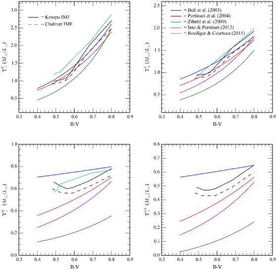
Figure 10: The $\Upsilon_{*}$ versus color relations for four bandpasses ($V$, $I$, $K$ and 3.6$\mu$m). The solid black line displays the results for the baseline model from Table 1 using a Kroupa IMF, dashed line is for a Chabrier IMF. Five models from the literature as also shown (Bell et al. 2003, Portinari et al. 2004, Zibetti et al. 2009, Into & Portinari 2013 and Roediger & Courteau 2015). Our current models agree in the optical bandpasses, but there is significant range in the near-IR bandpasses as outlined in McGaugh & Schombert (2014).

Figure 10 summarizes our baseline model comparison to other models in the literature from optical to near-IR bandpasses. The Bell et al. (2003), Portinari et al. (2004), Zibetti et al. (2009) and Into & Portinari (2013) studies were discussed in McGaugh & Schombert (2014). They all use a variety of IMF’s and AGB prescriptions (outlined in McGaugh & Schombert 2014, Table 5). New to our comparisons is the study by Roediger & Courteau (2015) which uses the newer population models also used in this study. The difference in the optical $\Upsilon_{*}$ values are primarily due to different assumptions in the SFH of the models. Despite the variance in SFH assumptions, the $\Upsilon_{*}$ values are very similar and follow the same trends with color. The near-IR $\Upsilon_{*}$ models diverge significantly, primarily on changes to the treatment of AGB’s and updated isochrones. Roediger & Courteau use the same isochrones as this study and produce similar $K$ values (they did not investigate $Spitzer$ bandpasses).

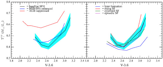
Figure 11: A comparison of the effects of different stellar population parameters and SFH’s on $\Upsilon_{*}$ at 3.6$\mu$m. The various models are discussed in the text. While most studies predict similar $\Upsilon_{*}$ values in the optical bandpasses, they all diverge at near-IR bandpasses due to varying prescriptions on later SFH effects and AGB treatment. The shade area defines a region for models where the final SFR and final [Fe/H] values were varied by 2$\sigma$ from their deduced values in the MSg and mass-metallicity relations.

The variations in model assumptions outlined in Figures 8 and 9 are presented in how they effect $\Upsilon_{*}$ in Figure 11. The baseline model, as outlined in Table 1, are displayed as the solid black line. In addition, the baseline models were expanded to consider different values for final SFR and [Fe/H] where at a particular stellar mass we vary the SFR and [Fe/H] to cover a 2$\sigma$ change in the MSg and mass-metallicity relations. The change in color is primarily driven by metallicity, so these dispersion models track the [Fe/H] vector in color space, but can be significant in $\Upsilon_{*}$ estimates as shown by the colored regions in Figure 11. Second order polynomial fits to the baseline models, across all the colors in the sample, are listed in Table 2. Also found in Table 2 is the mean value for a solar metallicity galaxy (i.e., one at the turnoff point in the MSg, or $10^{10}$ $M_{\sun}$).

Changes in the assumed stellar population parameters, such as the fraction of BHB, BSs and AGB stars have the obvious effects. BHB and BSs stars, which have a significant effect on optical colors, but do not have a noticeable change on the $\Upsilon_{*}$ values at 3.6$\mu$m. The absence of a significant fraction of AGB stars has a large effect on $\Upsilon_{*}$ as the 3.6$\mu$m where luminosity decreases by 20%. As this AGB absence is noted in CMD diagrams of nearby LSB dwarfs, this is a concern for accurate $\Upsilon_{*}$ estimates for low SFR dwarfs (the high SFR dwarfs, such as the ANGST sample, do not display this deficiency).

The right panel in Figure 11 displays variation in the assumed SFH as discussed in §4. All the considered scenarios result in lower $\Upsilon_{*}$ values compared to the baseline scenario. The later and extended SF scenarios have lower mean $\Upsilon_{*}$ (of about 0.1 dex) due to the fact that both these scenarios input higher fractions of younger stars compared to the other scenarios. Decreasing the SFR in the past would move the mean $\Upsilon_{*}$ upward, but this would place these scenarios in tension with the main sequence results, in that the total star formation rate needs to be lower to reproduce the correct final stellar masses which, typically, alters the predicted slope of the MSg. As the slope of the MSg is the least well defined aspect to star-forming galaxies, there is some leeway in possible star formation histories.

If the deficiency in AGB stars for LSB dwarf is confirmed, then the decrease in $\Upsilon_{*}$ by later or extended SFH’s is offset by the bottom heavy nature of AGB-light stellar populations. This may explain the conclusion from Schombert & McGaugh (2014) on the surprising stability of $\Upsilon_{*}$ as a free parameter in fits to the radial acceleration relation as population effects are balanced by SFH scenario changes for lower mass galaxies.

Lastly, we note, for accurate mass models, population gradients can play a role. In particular, the need to adjust $\Upsilon_{*}$ for a bulge component. As noted in Figure 8, the addition of a bulge component to a solar metallicity model, by B/D ratio to colors, exactly matches the red end of the two color diagram. The effect on $\Upsilon_{*}$ would be effective raising the value of the reddest galaxies from 0.6 to 0.7 for the early-type spirals, and 0.8 for S0 galaxies.

6.4 Uncertainties in $\Upsilon_{*}$ Models

While having $\Upsilon_{*}$ to color relationships, such as Figure 11, are the ultimate goal for obtaining stellar mass from a luminosity value, the correct application of this value requires knowledge of their accuracy and uncertainty. Accuracy, in this context, refers to the effect that observational error (in this case, the error in the observed galaxy color) has on the $\Upsilon_{*}$ value. Uncertainty refers to the range in $\Upsilon_{*}$ values for a reasonable range in model parameters for the particular galaxy color or mass.

Accuracy is relatively easy to calculate. For a known error in color, one searches for the two models that satisfy the upper and low bounds in color (i.e., the $\Upsilon_{*}$ values for two $V-3.6$ colors in Figure 11). This range will be higher for bluer colors (e.g., $B-V$ in Figure 10), which is why near-IR colors are preferred for $\Upsilon_{*}$ work. For typical near-IR color errors in the 0.05 range, the resulting errors in $\Upsilon_{*}$ (at 3.6) were 0.04.

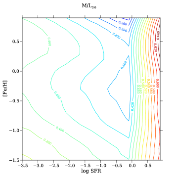
Figure 12: The range of calculated $\Upsilon_{*}$ values for models with a range of current SFR and metallicities (the two defining model inputs where SFR defines the SFH shape, and therefore the ages of the underlying stellar population, and current metallicity which defines the chemical enrichment mode, and therefore the metallicity distribution in the underlying stellar population). The more compressed contours above log SFR = 0 reflects the shallower slope to the high-mass MSg, which drives an older stellar populations from stronger and earlier star formation. Below log SFR = 0, the models and deduced $\Upsilon_{*}$ values are robust to small errors in the MSg and mass-metallicity relations (see text).

Uncertainty questions the validity of a particular model to a particular galaxy color or mass. This, unsurprisingly, has a larger impact on $\Upsilon_{*}$ values than color errors. Uncertainty in the models reflects either error in the choice of the input parameters (in our scenarios, current SFR and metallicity) or inappropriate choice of stellar population parameters (e.g., an enhanced BHB scenarios). The latter, choice of population parameters, results in a discrete shift in $\Upsilon_{*}$ values (see Figure 10) and can not quantified as error on $\Upsilon_{*}$. However, error in the input parameters does reflect a inherent unknown from the scatter in the MSg plus mass-metallicity relation. Dispersion in the measured current SFR produces a range in deduced SFH. Range in assumed metallicity alters the chemical enrichment model. Both can have significant effects on the final deduced galaxy colors.

To access the impact on the scatter in the MSg and mass-metallicity relation, we can consult a $\Upsilon_{*}$ contour plot such as shown in Figure 12. Here a range of SFR and [Fe/H] values are plotted with their resulting $\Upsilon_{*}$ values. The SFR value contains two uncertainties, the scatter in the MSg relation in the SFR direction plus the scatter in total stellar mass (since the integrated SFH from the SFR value produces the total stellar mass). However, the total stellar mass error is small (small changes in $\Upsilon_{*}$ with SFR) and can be iterated.

As noted in §2, the scatter in the MSg is around 0.4 dex on the low-mass end and around 0.1 on the high-mass end. While the scatter in the mass-metallicity relation is around 0.3 dex (increasing to lower galaxy masses). For particular regions in Figure 12 this can mean the model $\Upsilon_{*}$ values are robust (e.g., below log SFR = $-$1) or increasingly sensitive to the assumed SFR value (e.g., above log SFR = 0).

7 Summary

The premise of this study is that knowledge of the SFH in star-forming galaxies as given by the main sequence relation, combined with present-day colors and flexible stellar population models, allows for an understanding of the underlying stellar population in terms of their total mass and luminosity. Previous studies have indicated that the mass-to-light ratio ($\Upsilon_{*}$) varies with the rate of star formation, but that this maps smoothly into galaxy color, which is driven by the same population changes that reflect into $\Upsilon_{*}$.

Completely accurate knowledge of the distribution of age and metallicity of stars in star-forming galaxies will be an elusive goal. However, the numerical experiments in §5 and §6 indicate the range of possible SFH’s is fairly narrow plus results in a similar distributions of the various types of stars that dominate galaxy colors. This narrow range in stellar populations also reflects into well defined color-$\Upsilon_{*}$ relations from which an accurate mass-to-light ratio can be extracted across most optical and near-IR bandpasses.

Our conclusions can be summarized as follows:

• The main sequence for star-forming galaxies divides into two parts (see Figure 1); 1) the high-mass end (weary giants, $M_{*}>10^{10.5}M_{\sun}$) which has been investigated with redshift and has a shallow slope (Speagle et al. 2014), and 2) the low-mass end (thriving dwarfs, $M_{*}<10^{10.5}M_{\sun}$), explored by McGaugh, Schombert & Lelli (2017) and Cook et al. (2014), which has a steeper slope, parallel to a line of constant SF over time and is sub divided by $FUV-NUV$ color. The division by UV colors across the line of constant SF signals a separation between galaxies with declining versus rising SFR over that last Gyr.

• The various color locus for star-forming galaxies has coherence across bandpasses (i.e., red galaxies are red in all colors), but has a great deal of scatter in excess of the observational error suggesting a wide variance in age and metallicity. The fact that color divides nominally by galaxy stellar mass (see Figure 2) implies that metallicity is the strongest driver for color with increasing importance to recent SF at the low-mass end.

• The SFH of the high-mass end of the MSg is well-defined by the study of Speagle et al. (2014). This can be qualified, roughly, as a moderate, wide initial burst of SF with a shallow decline to the present epoch. To reproduce the high-mass end of the MSg, this decline must be steeper with increasing final stellar mass. In adopting a similar SFH shape for the low-mass end of the MSg, one must have a slightly longer initial burst with nearly constant SFR at the inflection point of $10^{10.}M_{\sun}$ with slightly declining SFH with lower mass (see Figure 3). These are the baseline SFH used in Table 1; however, a range of different SFH can produce the same slope on the low-mass end of the MSg (see Figure 5) but produce different color and metallicity relations.

• Stellar population models mix age (the assumed SFH) and metallicity (the assumed chemical enrichment model) to produce a composite stellar population that generates the observed integrated luminosity and colors. Of the many components to a stellar population, one is critical to $\Upsilon_{*}$ (the IMF) and two are critical to galaxy colors (AGB treatment and the BHB+BSs component). With respect to the low-mass end of the MSg and near-IR colors, the AGB component, while matching LMC/SMC cluster colors, appears deficient in some LSB galaxies (Schombert & McGaugh 2015) and enhanced in other star-forming dwarfs (Dalcanton et al. 2009). In a similar fashion, an enhanced BHB+BSs population (expected at low metallicities) alters, significantly, the optical colors. In order to match the galaxy color locus (Figure 8), baseline stellar populations are adequate, but enhanced AGB and/or enhanced BHB+BSs components are required at the low-mass end.

• Variations in SFH scenarios, within limits to maintain the slope and zeropoint of the MSg, do not produce large variations in galaxy colors (see Figure 9). Recent SF can drive optical colors to very blue values ($B-V<0.4$), but changes in near-IR colors are difficult to reproduce with different SFH scenarios.

• Existing $\Upsilon_{*}$ versus color relationships in the literature converge in their predictions in optical bandpasses (McGaugh & Schombert 2014), but are wildy discrepant in the near-IR bandpasses (see Figure 10). Recent models (such as Roediger & Courteau 2015) offer a more coherent view in the near-IR due to improved treatment of intermediate aged stars. Our baseline models predict nearly constant $\Upsilon_{*}$ with color in the near-IR, with the most significant effect being the choice of the IMF (with a variation of 0.1 dex between bottom heavy versus bottom light scenarios).

• Blending stellar population components, IMF effects and SFH scenarios produces the estimates displays in Figure 11, where $\Upsilon_{*}$ can be estimated with a single optical to near-IR color. The dispersion on $\Upsilon_{*}$ can be estimated as a function of stellar population effects (left panel) versus SFH effects (right panel). The color region in Figure 11 provides some guidance for a nominal change in the input parameters as given by the uncertainty in the MSg and the mass-metallicity relations. Aside from radical departures from estimates of the contribution from AGB stars or extremely later epoch’s of initial star formation, all the considered scenarios fall within the baseline model’s zone of variance. A simplistic, first-order description for the baseline model is constant $\Upsilon_{*}[3.6]$ (approximate 0.45) until a galaxy color of $V-3.6=2.8$ followed by a linear rise to elliptical value of 0.7 by the reddest colors of 3.2. These models and a $\Upsilon_{*}$ calculator is available at the SPARC website.

The model determination of $\Upsilon_{*}$ at various bandpasses is critical to many low and high redshift studies of stellar mass in galaxies. A well studied model from the UV to near-IR allows for an application to high redshift systems which will account for redshifted filters as well as different epochs being sampled with cosmic time. The zero redshift models are important as applied to the baryon Tully-Fisher relation (McGaugh 2012) and the radial acceleration relation (McGaugh, Lelli & Schombert 2016). These models form the core of our future studies to convert galaxy photometry into stellar masses to study the relation between baryons and dark matter.

Appendix A $\Upsilon_{*}$ Webtool

The range of metallicities and different population parameters makes a tabulated presentation of the models impossible. Instead, a webtool is offered the community (http://abyss.uoregon.edu/$\sim$js/sfh) to provide either 1) colors and $\Upsilon_{*}$ values per galaxy stellar mass or 2) a user selected $V-3.6$ color value and error.

The first option has two paths. First, the user can enter either a SFR, galaxy stellar mass ($M_{*}$) or final metallicity ([Fe/H]). The webtool will then convert any of the three parameters into the other two using the MSg and mass-metallicity relation discussed in the text (see Table 1). The total stellar mass determines the rate of chemical evolution (slow, normal or fast, see §5.1). The selected SFR determines the SFH input to the models. The selected final [Fe/H] value plus enrichment model determines the metallicity at any particular epoch. The user can override the values deduced from the main sequence and mass-metallicity relations by selecting their own SFR, [Fe/H] and chemical enrichment values, although the physical validity of many possible combinations is questionable.

A second option is to enter a $V-3.6$ color and uncertainty in that color. The webtool will present the best fit model for that color, and the range in $\Upsilon_{*}$ values due to the uncertainty in the color. This always assumes the standard SFR and [Fe/H] values outlined in the text (see Table 1).

Lastly, the user can adjust any of the above models for various enhancements in the underlying stellar populations (e.g., AGB, BHB, BSs populations). These models will continue to apply standard SFR and [Fe/H] values per stellar mass, but use altered stellar population parameters discussed in §5. Again, the meaning and value of many of these extreme models is up to the user to decide.

References

- Abramson et al. (2016) Abramson, L. E., Gladders, M. D., Dressler, A., et al. 2016, ApJ, 832, 7.
- de Vaucouleurs et al. (1991) de Vaucouleurs, G., de Vaucouleurs, A., Corwin, H. G., Jr., et al. 1991, Third Reference Catalogue of Bright Galaxies.
- Bailyn (1995) Bailyn, C. D. 1995, ARA&A, 33, 133
- Bell & de Jong (2000) Bell, E. F., & de Jong, R. S. 2000, MNRAS, 312, 497
- Bell, et al. (2003) Bell, E. F., McIntosh, D. H., Katz, N., et al. 2003, The Astrophysical Journal Supplement Series, 149, 289.
- Bernardi et al. (2017) Bernardi, M., Meert, A., Sheth, R. K., et al. 2017, MNRAS, 467, 2217
- Brown et al. (2018) Brown, T., Cortese, L., Catinella, B., & Kilborn, V. 2018, MNRAS, 473, 1868
- Bruzual & Charlot (2003) Bruzual, G., & Charlot, S. 2003, MNRAS, 344, 1000
- Bruzual (2009) Bruzual, A. G. 2009, ArXiv e-prints , arXiv:0911.0791.
- Bruzual A. (2010) Bruzual A., G. 2010, Philosophical Transactions of the Royal Society of London Series A, 368, 783
- Calzetti (2001) Calzetti, D. 2001, PASP, 113, 1449
- Cano-Díaz, et al. (2016) Cano-Díaz, M., Sánchez, S. F., Zibetti, S., et al. 2016, ApJ, 821, L26.
- Cappellari et al. (2006) Cappellari, M., Bacon, R., Bureau, M., et al. 2006, MNRAS, 366, 1126
- Cassisi et al. (2004) Cassisi, S., Salaris, M., Castelli, F., & Pietrinferni, A. 2004, ApJ, 616, 498
- Chabrier (2003) Chabrier, G. 2003, ApJ, 586, L133
- Charlot & Fall (2000) Charlot, S., & Fall, S. M. 2000, ApJ, 539, 718
- Cohen, et al. (2007) Cohen, J. G., Hsieh, S., Metchev, S., et al. 2007, AJ, 133, 99.
- Conroy et al. (2009) Conroy, C., Gunn, J. E., & White, M. 2009, ApJ, 699, 486
- Conroy & Gunn (2010) Conroy, C., & Gunn, J. E. 2010, ApJ, 712, 833
- Conroy & van Dokkum (2012) Conroy, C. & van Dokkum, P. G. 2012, ApJ, 760, 71.
- Conroy et al. (2009) Conroy, C., Gunn, J. E., & White, M. 2009, ApJ, 699, 486
- Conroy et al. (2010) Conroy, C., White, M., & Gunn, J. E. 2010, ApJ, 708, 58
- Cook et al. (2014) Cook, D. O., Dale, D. A., Johnson, B. D., et al. 2014, MNRAS, 445, 899
- Cortese, et al. (2017) Cortese, L., Catinella, B. & Janowiecki, S. 2017, ApJ, 848, L7.
- Daddi et al. (2007) Daddi, E., Dickinson, M., Morrison, G., et al. 2007, ApJ, 670, 156
- Dalcanton et al. (2009) Dalcanton, J. J., Williams, B. F., Seth, A. C., et al. 2009, ApJS, 183, 67
- Eskew et al. (2012) Eskew, M., Zaritsky, D., & Meidt, S. 2012, AJ, 143, 139
- Gallazzi & Bell (2009) Gallazzi, A., & Bell, E. F. 2009, ApJS, 185, 253
- Gonzalez-Perez, et al. (2014) Gonzalez-Perez, V., Lacey, C. G., Baugh, C. M., et al. 2014, MNRAS, 439, 264.
- Guiderdoni & Rocca-Volmerange (1987) Guiderdoni, B., & Rocca-Volmerange, B. 1987, A&A, 186, 1
- Haywood, et al. (2018) Haywood, M., Di Matteo, P., Lehnert, M., et al. 2018, ArXiv e-prints , arXiv:1802.09887.
- Hurley et al. (2002) Hurley, J. R., Tout, C. A., & Pols, O. R. 2002, MNRAS, 329, 897
- Into & Portinari (2013) Into, T., & Portinari, L. 2013, MNRAS, 430, 2715
- Jarrett (2000) Jarrett, T. H. 2000, PASP, 112, 1008
- Jaskot et al. (2015) Jaskot, A. E., Oey, M. S., Salzer, J. J., et al. 2015, ApJ, 808, 66
- Jimenez & Padoan (1998) Jimenez, R., & Padoan, P. 1998, ApJ, 498, 704
- Kennicutt & Evans (2012) Kennicutt, R. C., & Evans, N. J. 2012, ARA&A, 50, 531
- Ko et al. (2013) Ko, Y., Lee, M. G., & Lim, S. 2013, ApJ, 777, 82
- Kroupa (2001) Kroupa, P. 2001, MNRAS, 322, 231
- Kurczynski et al. (2016) Kurczynski, P., Gawiser, E., Acquaviva, V., et al. 2016, ApJ, 820, L1
- Kyeong et al. (2003) Kyeong, J.-M., Tseng, M.-J., & Byun, Y.-I. 2003, A&A, 409, 479
- Lee et al. (2018) Lee, J. H., Pak, M., Lee, H.-R., & Oh, S. 2018, ApJ, 857, 102
- Leitner (2012) Leitner, S. N. 2012, ApJ, 745, 149.
- Lelli et al. (2016) Lelli, F., McGaugh, S. S., & Schombert, J. M. 2016, AJ, 152, 157
- Lelli, et al. (2017) Lelli, F., McGaugh, S. S., Schombert, J. M., et al. 2017, ApJ, 836, 152.
- Li & Han (2008) Li, Z., & Han, Z. 2008, MNRAS, 387, 105
- López-Sanjuan, et al. (2018) López-Sanjuan, C., Díaz-García, L. A., Cenarro, A. J., et al. 2018, ArXiv e-prints , arXiv:1805.03609.
- Maraston (2005) Maraston, C. 2005, MNRAS, 362, 799
- Matteucci (2007) Matteucci, F. 2007, From Stars to Galaxies: Building the Pieces to Build Up the Universe, 374, 89
- McCrea (1964) McCrea, W. H. 1964, MNRAS, 128, 147
- McGaugh (2012) McGaugh, S. S. 2012, AJ, 143, 40
- McGaugh & Schombert (2014) McGaugh, S. S., & Schombert, J. M. 2014, AJ, 148, 77
- McGaugh et al. (2017) McGaugh, S. S., Schombert, J. M., & Lelli, F. 2017, ApJ, 851, 22
- McGaugh (1991) McGaugh, S. S. 1991, ApJ, 380, 140
- McGaugh et al. (2016) McGaugh, S. S., Lelli, F., & Schombert, J. M. 2016, Physical Review Letters, 117, 201101
- McGaugh et al. (2017) McGaugh, S. S., Schombert, J. M., & Lelli, F. 2017, ApJ, 851, 22
- McQuinn et al. (2010) McQuinn, K. B. W., Skillman, E. D., Cannon, J. M., et al. 2010, ApJ, 724, 49
- McWilliam (1997) McWilliam, A. 1997, ARA&A, 35, 503
- Medling et al. (2018) Medling, A. M., Cortese, L., Croom, S. M., et al. 2018, MNRAS, 475, 5194
- Meidt et al. (2014) Meidt, S. E., Schinnerer, E., van de Ven, G., et al. 2014, ApJ, 788, 144
- Milgrom (2009) Milgrom, M. 2009, Phys. Rev. D, 80, 123536
- Milone et al. (2010) Milone, A., Sansom, A. E., & Sánchez-Blázquez, P. 2010, Stellar Populations - Planning for the Next Decade, 262, 394
- Morrissey et al. (2007) Morrissey, P., Conrow, T., Barlow, T. A., et al. 2007, ApJS, 173, 682
- Murphy et al. (2011) Murphy, E. J., Condon, J. J., Schinnerer, E., et al. 2011, ApJ, 737, 67
- Noeske et al. (2007) Noeske, K. G., Weiner, B. J., Faber, S. M., et al. 2007, ApJ, 660, L43
- Norris et al. (2016) Norris, M. A., Van de Ven, G., Schinnerer, E., et al. 2016, ApJ, 832, 198
- Pagel (1997) Pagel, B. E. J. 1997, Nucleosynthesis and Chemical Evolution of Galaxies, by Bernard E. J. Pagel, pp. 392. ISBN 0521550610. Cambridge, UK: Cambridge University Press, October 1997., 392
- Parikh et al. (2018) Parikh, T., Thomas, D., Maraston, C., et al. 2018, MNRAS, 477, 3954.
- Peng et al. (2010) Peng, Y.-j., Lilly, S. J., Kovač, K., et al. 2010, ApJ, 721, 193
- Peng et al. (2015) Peng, Y., Maiolino, R., & Cochrane, R. 2015, Nature, 521, 192
- Pessev et al. (2006) Pessev, P. M., Goudfrooij, P., Puzia, T. H., & Chandar, R. 2006, AJ, 132, 781
- Pildis et al. (1997) Pildis, R. A., Schombert, J. M., & Eder, A. 1997, ApJ, 481, 157
- Portinari et al. (2004) Portinari, L., Sommer-Larsen, J., & Tantalo, R. 2004, MNRAS, 347, 691
- Prantzos (2009) Prantzos, N. 2009, The Galaxy Disk in Cosmological Context, 254, 381
- Preston & Sneden (2000) Preston, G. W., & Sneden, C. 2000, AJ, 120, 1014
- Querejeta et al. (2015) Querejeta, M., Meidt, S. E., Schinnerer, E., et al. 2015, ApJS, 219, 5
- Rix & Zaritsky (1995) Rix, H.-W. & Zaritsky, D. 1995, ApJ, 447, 82.
- Roediger & Courteau (2015) Roediger, J. C., & Courteau, S. 2015, MNRAS, 452, 3209
- Sandage, & Tammann (1981) Sandage, A., & Tammann, G. A. 1981, Washington: Carnegie Institution.
- Salim et al. (2007) Salim, S., Rich, R. M., Charlot, S., et al. 2007, ApJS, 173, 267
- Salpeter (1955) Salpeter, E. E. 1955, ApJ, 121, 161
- Sarajedini (2007) Sarajedini, A. 2007, Revista Mexicana de Astronomia y Astrofisica Conference Series, 29, 48
- Schombert & McGaugh (2014) Schombert, J., & McGaugh, S. 2014, Publ. Astron. Soc. Australia, 31, e036
- Schombert & McGaugh (2015) Schombert, J., & McGaugh, S. 2015, AJ, 150, 72
- Schombert & Rakos (2009) Schombert, J., & Rakos, K. 2009, AJ, 137, 528
- Schombert (2016) Schombert, J. M. 2016, AJ, 152, 214
- Schombert (2018) Schombert, J. M. 2018, AJ, 155, 69
- Sheth et al. (2010) Sheth, K., Regan, M., Hinz, J. L., et al. 2010, PASP, 122, 1397
- Smolčić et al. (2006) Smolčić, V., Ivezić, Ž., Gaćeša, M., et al. 2006, MNRAS, 371, 121
- Speagle et al. (2014) Speagle, J. S., Steinhardt, C. L., Capak, P. L., & Silverman, J. D. 2014, ApJS, 214, 15 P. R. M., Mainzer, A. K., et al. 2010, AJ, 140, 1868
- Taylor, et al. (2011) Taylor, E. N., Hopkins, A. M., Baldry, I. K., et al. 2011, MNRAS, 418, 1587.
- Thomas et al. (2004) Thomas, D., Maraston, C., & Korn, A. 2004, MNRAS, 351, L19
- Thomas et al. (2005) Thomas, D., Maraston, C., Bender, R., & Mendes de Oliveira, C. 2005, ApJ, 621, 673
- Trager et al. (2000) Trager, S. C., Faber, S. M., Worthey, G., & González, J. J. 2000, AJ, 120, 165
- Tremonti et al. (2004) Tremonti, C. A., Heckman, T. M., Kauffmann, G., et al. 2004, ApJ, 613, 898
- Verlinde (2016) Verlinde, E. P. 2016, ArXiv e-prints , arXiv:1611.02269.
- Villaume et al. (2015) Villaume, A., Conroy, C., & Johnson, B. D. 2015, ApJ, 806, 82
- Wright et al. (2010) Wright, E. L., Eisenhardt, P. R. M., Mainzer, A. K., et al. 2010, AJ, 140, 1868
- Wuyts et al. (2011) Wuyts, S., Förster Schreiber, N. M., van der Wel, A., et al. 2011, ApJ, 742, 96
- Zahid et al. (2011) Zahid, H. J., Kewley, L. J., & Bresolin, F. 2011, ApJ, 730, 137
- Zibetti et al. (2009) Zibetti, S., Charlot, S., & Rix, H.-W. 2009, MNRAS, 400, 1181