Extended polarized semiclassical model for quantum-dot cavity QED and its application to single-photon sources

Abstract

We present a simple extension of the semi-classical model for a two-level system in a cavity, in order to incorporate multiple polarized transitions, such as those appearing in neutral and charged quantum dots (QDs), and two nondegenerate linearly polarized cavity modes. We verify the model by exact quantum master equation calculations, and experimentally using a neutral QD in a polarization non-degenerate micro-cavity, in both cases we observe excellent agreement. Finally, the usefulness of this approach is demonstrated by optimizing a single-photon source based on polarization postselection, where we find an increase in the brightness for optimal polarization conditions as predicted by the model.

I introduction

Understanding the interaction of a two-level system, such as atomic transitions or excitonic transitions in a semiconductor quantum dot (QD), with an optical cavity mode, is key for designing efficient single photon sources (grange2015, ; somaschi_near-optimal_2016, ; ding_-demand_2016, ; wang2019g, ) and photonic quantum gates (imamoglu_strongly_1997, ) for quantum networks (kimble_quantum_2008, ). Traditionally, the interaction of a two-level quantum system with an electromagnetic mode is described by the Jaynes-Cummings model, which can be approximated in the so-called semi-classical approach, where the light field is treated classically and atom-field correlations are neglected. We focus here on QD-cavity systems in the weak coupling “bad cavity” regime $\left(g\ll\kappa\right)$. The transmission amplitude in the semi-classical approximation is given by (armen_low-lying_2006, ; waks_dipole_2006, ; auffeves-garnier_giant_2007, ; loo_optical_2012, ; majumdar2012c, ; hu_extended_2015, ; bakker_polarization_2015, )

$$t=\eta_{out}\frac{1}{1-2i\Delta+\frac{2C}{1-i\Delta^{{}^{\prime}}}}.$$ (1)

Here, $\eta_{out}$ is the probability amplitude that a photon leaves the cavity through one of the mirrors, we assume two identical mirrors. $\Delta=\left(f-f_{c}\right)/\kappa$ is the normalized detuning of the laser frequency $f$ with respect to the cavity resonance frequency $f_{c}$ and cavity loss rate $\kappa$, $\Delta^{\prime}=\left(f-f^{{}^{\prime}}\right)/\gamma_{\perp}$ is the normalized detuning with respect to the QD resonance frequency $f^{{}^{\prime}}$ and dephasing rate $\gamma_{\perp}=\frac{\gamma_{||}}{2}+\gamma^{*}$. $\Delta$ is related to the round trip phase $\phi$ by $\phi\approx\frac{2\pi\Delta}{\mathcal{{F}}}$ for small detuning $\Delta$, and $\mathcal{{F}}$ is the finesse of the cavity. The coupling of the QD to the cavity mode is given by the cooperativity parameter $C=\frac{g^{2}}{\kappa\gamma_{\perp}}$, where the QD-cavity coupling strength is $g$. In Appendix A, we show how Eq. 1 can be derived in a fully classical way. The main limitation of semi-classical models is that the population of the excited state is not taken into account, as well as phonon-assisted transitions, spin flips, and other interactions with the environment.

In this paper, Eq. (1) is extended to take into account two orthogonal linearly-polarized fundamental optical cavity modes, and multiple polarized QD transitions oriented at an arbitrary angle relative to the cavity polarization axes. This extension is important because it is experimentally very challenging to produce perfectly polarization degenerate micro-cavities (bonato_tuning_2009, ; frey_electro-optic_2018, ), and the slightly non-polarization degenerate case has attracted attention recently (anton_tomography_2017, ; he_polarized_2018, ; wang2019g, ). It is essential to have access to a good analytic model, for instance to numerically fit experimental data to derive the system parameters, or to optimize the performance of a single-photon source; this is very time-consuming using exact quantum master equation simulations. Exemplary code of our model is available online (snijders2018f, ). We compare our model to experimental data as well as numerical solutions of the quantum master equation, and we demonstrate that it can be used to significantly increase the brightness of a single-photon source. We focus here on Fabry-Perot type QD-cavity systems but our results are valid for a large range of cavity QED systems.

II Extended semi-classical model

To start the analysis, we show in Fig. 1 a sketch of a polarized QD-cavity system with two cavity modes (H,V) and two QD dipole transitions (X,Y). In order to demonstrate the complexity of the transmission spectrum that appears is this case, we show in the inset of Fig. 1 the transmission of linearly polarized input light $\left(\theta_{in}=45^{\circ}\right)$ as a function of the relative laser frequency $\Delta f$.

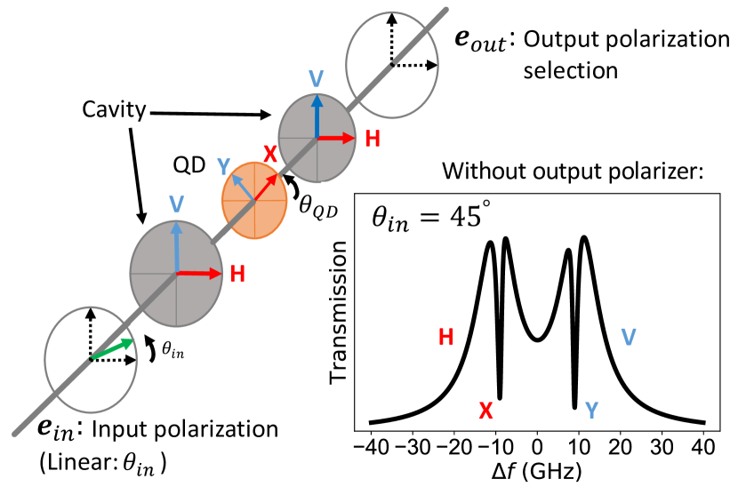
Figure 1: Sketch of a polarized cavity–neutral QD system. H and V denote the linearly polarized cavity modes, X and Y represent the dipole polarization axes of the QD at an angle $\theta_{QD}$ with respect to the H cavity polarization, and $\mathbf{e}_{in}$ and $\mathbf{e}_{out}$ indicate the incident polarization and output polarization postselection. The inset shows the transmission spectrum calculated with the extended semiclassical model for incident linear polarized light ($\theta_{in}=45^{\circ}$). The difference in dip depth between the X and Y transitions is due to the specific QD dipole orientations ($\theta_{QD}$). Here, no polarization postselection is done. The parameters are $f_{H}=-10\,$GHz, $f_{V}=10\,$GHz, $f_{X}^{{}^{\prime}}=-9\,$GHz, $f_{Y}^{{}^{\prime}}=9\,$GHz, $\theta_{QD}=10^{\circ}$.

We now show how Eq. 1 can directly be extended to take care of all polarization effects, by replacing the scalar quantities by appropriate Jones vectors and matrices. To motivate the precise form, we first write Eq. 1 as its Taylor expansion

$$\begin{array}[]{c}t=\eta_{out}\left[1+\left(-2i\Delta+\frac{2C}{1-i\Delta^{{}^{\prime}}}\right)+\right.\\ \left.\left(-2i\Delta+\frac{2C}{1-i\Delta^{{}^{\prime}}}\right)^{2}+\cdots\right],\end{array}$$

where we now can clearly identify contributions from the cavity and from the QD. This form reminds us of the multiple roundtrips happening in a Fabry-Perot cavity, we show a complete derivation of Eq. 1 in the Appendix. In the polarization basis of the cavity, the normalized detuning phase $2i\Delta$ becomes the Jones matrix

$$\left(\begin{array}[]{cc}2i\Delta_{H}&0\\ 0&2i\Delta_{V}\end{array}\right),$$ (2)

where $\Delta_{m}=\left(f-f_{m}\right)/\kappa_{m}$ for $m=H,V$ are the normalized laser detunings from the polarized cavity resonances at frequencies $f_{m}$. The interaction with the QD modifies the round-trip phase, but because of a possible misalignment of the dipole axes of the QD transitions and the cavity polarization basis, we have to calculate the QD effect in its own basis, which is accomplished by $R_{-\theta_{QD}}XR_{\theta_{QD}}$, where $R_{\theta_{QD}}$ is the 2D rotation matrix and $\theta_{QD}$ the rotation angle between the cavity and quantum dot frame, see Fig. 1. There are many different transitions possible in QDs (bayer_fine_2002, ; warburton_single_2013, ). This can be described by a transmission matrix $X$ composed of the appropriate Jones matrices $J_{n}$ (see Table 2.1 in (fowles_introduction_1989, )) and the Lorentzian frequency-dependent phase shifts $\phi_{n}$:

$$X=\sum_{n}J_{n}\varphi_{n}=\sum_{n}J_{n}\frac{2C_{n}}{1-i\Delta_{n}^{{}^{\prime}}},$$ (3)

$\Delta_{n}^{{}^{\prime}}=\left(f-f_{n}^{{}^{\prime}}\right)/\gamma_{\perp n}$ are the normalized laser detunings from the QD resonances at $f_{n}^{{}^{\prime}}$, and $C_{n}$ are their cooperativity parameters. The case discussed here is that of a neutral QD exciton, where $X=\varphi_{H}H+\varphi_{V}V$ which is equal to Eq. 2. Note that, due to the nature of semi-classical models, nonlinear (such as electromagnetically induced transparency, EIT) and non-resonant effects (such as spin relexation and phonon interactions) are not reproduced. The resulting polarized Taylor-expanded expression for the transmission of the QD-cavity system is then given by

$$\begin{array}[]{c}t_{tot}=\eta_{out}\left[I_{2\times 2}+\left(-\left(\begin{array}[]{cc}2i\Delta_{H}&0\\ 0&2i\Delta_{V}\end{array}\right)+R_{-\theta_{QD}}XR_{\theta_{QD}}\right)+\right.\\ \left.\left(-\left(\begin{array}[]{cc}2i\Delta_{H}&0\\ 0&2i\Delta_{V}\end{array}\right)+R_{-\theta_{QD}}XR_{\theta_{QD}}\right)^{2}+\cdots\right].\end{array}.$$

Finally, we perform the reverse Taylor expansion, and obtain the full transmission amplitude matrix, which is the main result of this paper:

$$t_{tot}=\eta_{out}\left[I_{2\times 2}-\left(\begin{array}[]{cc}2i\Delta_{H}&0\\ 0&2i\Delta_{V}\end{array}\right)+R_{-\theta_{QD}}XR_{\theta_{QD}}\right]^{-1}.$$ (4)

Note that this result could have been directly obtained by plugging in the appropriate matrix expressions into Eq. 1. Experimentally most relevant is the scalar transmission amplitude for the case that the cavity-QED system is placed between an input and output polarizer. This can be obtained by $\mathbf{e}_{out}^{T}t_{tot}\mathbf{e}_{in}$, where $\mathbf{e}_{in}=\left(E_{in}^{H},E_{in}^{V}\right)^{T}$ and $\mathbf{e}_{out}=\left(E_{out}^{H},E_{out}^{V}\right)^{T}$ are the input and output Jones vectors or polarizations, also shown in the published code examples (snijders2018f, ).

We now compare our model to experiments and exact numerical simulations of the quantum master equation using QuTiP (johansson_qutip:_2012, ; johansson_qutip_2013, ), for a neutral QD in a polarization non-degenerate cavity. The device consists of a micropillar cavity with an embedded self-assembled QD (snijders_purification_2016, ). In Fig. 2, a false color plot of the measured transmission as a function of the relative laser detuning and the orientation of linearly polarized input laser is shown. By careful fitting of our model to the experimental data we obtain excellent agreement (see Fig. 2) using the following parameters: $\theta_{QD}=94^{\circ}\pm 2^{\circ}$, cavity splitting $f_{V}-f_{H}=10\pm 0.1$ GHz, QD fine-structure splitting $f_{Y}^{{}^{\prime}}-f_{X}^{{}^{\prime}}=2\pm 0.1$ GHz, $\kappa=11.1\pm 0.1$ GHz, $g=1.59\pm 0.08$ GHz and $\gamma_{\parallel}=0.32\pm 0.15$ GHz ($\gamma^{*}$ set to zero). From this, we obtain for both transitions the cooperativity $C=1.42\pm 0.5.$ Inserting these parameters in the quantum master equation for this system (snijders_purification_2016, ) we again find excellent agreement (see Fig. 2). In Appendix C we show that, for low mean photon number, the numerical results from the quantum master equation are equal to our extended semi-classical approach.

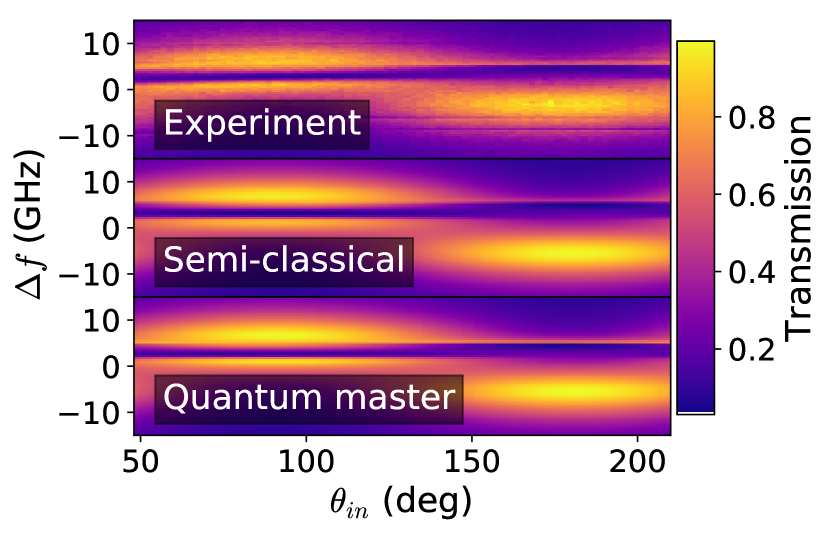
Figure 2: False color plots of the cavity transmission as function of laser frequency and linear input polarization orientation. The three false color plots show the experimental data, corrected for reduced detection efficiency, polarized semi-classical theory results based on Eq. (4) and numerical simulations based on the quantum master model.

III Application to single photon sources

Now we show that our model can be used to optimize the polarization configuration for quantum-dot based single-photon sources, in particular the single-photon purity (determined by the second-order correlation $g^{2}(0)$), and the brightness. To calculate $g^{2}(0)$, we need to take into account two contributions: First, single-photon light that has interacted with the QD, $\rho^{sp}(x)=x\left|1\right\rangle\left\langle 1\right|+\left(1-x\right)\left|0\right\rangle\left\langle 0\right|$, where $x$ is the mean photon number. Second, “leaked” coherent laser light, $\rho^{coh}(\alpha)$, with the mean photon number, $\left\langle n^{coh}\right\rangle=\left|\alpha\right|^{2}$, where $\left|\alpha\right|^{2}$ can be determined by tuning the QD out of resonance. With a weighting parameter, $\xi$, the density matrix of the total detected light can be written as

$$\rho^{tot}=\left[\xi\rho^{sp}(x)+(1-\xi)\rho^{coh}(\alpha)\right].$$ (5)

After determining $\rho^{tot}$, it is straightforward to obtain $g^{(2)}(0)$ of the total transmitted light (proux_measuring_2015, ).

To find the optimal polarization condition, we numerically optimize the input and output polarization, as well as the quantum dot and laser frequency, in order to maximize the light that interacted with the QD transition (single photon light), and to minimize the residual laser light. This is easily feasible because calculation of the extended semiclassical model is fast. We compare the optimal result to the conventional polarization conditions 90Cross (excitation of the H- and detection along the V-cavity mode) and “45Circ”. For 45Circ, the system is excited with $45^{\circ}$ linear polarized light and we detect a single circular polarization component. This works because, in this configuration, the birefringence of the cavity modes functions as a quarter wave plate. Fig. 3 compares the theoretical prediction to the experimental data for these cases, each with and without the QD. These results show almost perfect agreement between experiment and theory. Only for the 90Cross configuration, the experimental data is slightly higher than expected, which we attribute to small changes of the polarization axes of the QD induced by the necessary electrostatic tuning of the QD resonance.

The optimal polarization condition is found for the input polarization Jones vector $\mathbf{e}_{in}=\left(\begin{array}[]{cc}0.66,&0.50-0.57i\end{array}\right)^{T}$ and output polarization $\mathbf{e}_{out}=\left(\begin{array}[]{cc}0.66,&0.50+0.57i\end{array}\right)^{T}$. For this case, the single photon intensity is about $3\times$ higher compared to the 90Cross configuration. We emphasize that this optimal configuration can hardly be found experimentally because the parameter space, polarization conditions and QD and laser frequencies, is too large. Instead, numerical optimization has to be done, for which a simple analytical model, like the one presented here, is essential. Again we compare our extended semi-classical model to exact numerical simulations from the QuTiP to verify the validity of our model and the experimental results (see Fig. 3). Because here, the complex transmission amplitudes of both polarizations interfere, we can conclude from the good agreement that not only the transmission but also the transmission phases of Eq. 4 are correctly reproduced by the model.

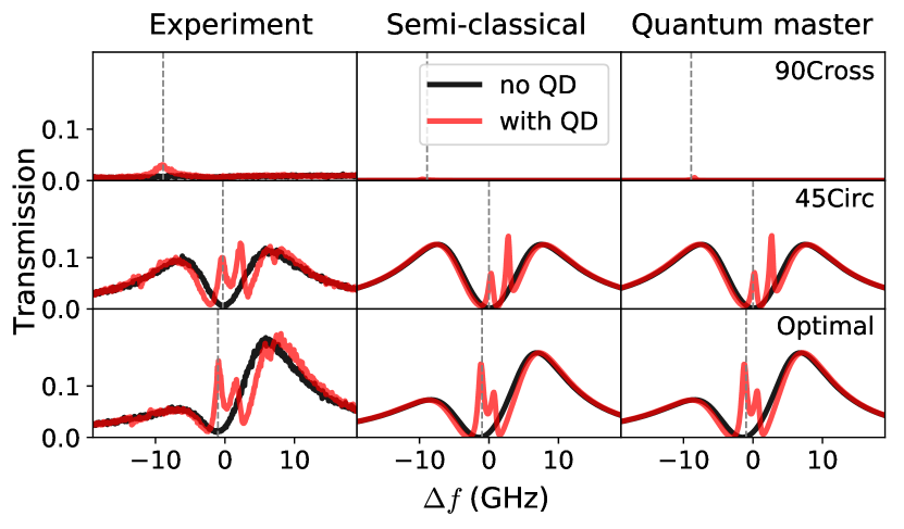
Figure 3: Measured (left), semi-classical simulated (middle) and quantum master simulated(right) transmitted intensity as a function of the relative laser frequency, with and without the QD, and for the three polarization configurations 90Cross (top), 45Circ (center), and Optimal (bottom). For constant laser power, the measured single-photon intensity (frequency indicated by the dashed vertical line) of the optimal configuration is about $3\times$ ($1.6\times$) higher compared to the 90Cross (45Circ) configuration.

For the configurations shown in Fig. 3, we now perform power-dependent continuous-wave measurements to determine the experimental brightness and $g^{(2)}(0)$. The laser is locked at the optimal frequency determined by the model (dashed vertical line in Fig. 3), and the single photon count rate, as well as the second-order correlation function, is measured using a Hanbury-Brown Twiss setup. The photon count rate is the actual count rate before the first lens, corrected for reduced detection efficiency. Gaussian fits to $g^{(2)}(\tau)$ are used to determine the second-order correlation function at zero time delay $g^{(2)}(0)$.

In Fig. 4(a), the single-photon count rate is shown as a function of the input power, and in Fig. 4(b) we show $g_{exp}^{(2)}(0)$ as a function of the single-photon count rate. In Fig. 4(b), we see that, for the optimal configuration, the single photon rate can be up to 24 MHz before the purity of the single-photon source decreases. This means that, for the same purity, it is possible to increase the brightness of the single-photon source by using different input and output polarization configurations. Note that $g_{exp}^{2}(0)\approx 0.5$ corresponds to a real $g^{(2)}(0)\approx 0$ due to detector jitter. The two-detector jitter of $\approx 500$ ps, which is of the same order as the the cavity enhanced QD decay rate, explains the limited lower value of $g_{exp}^{(2)}(\tau)$.

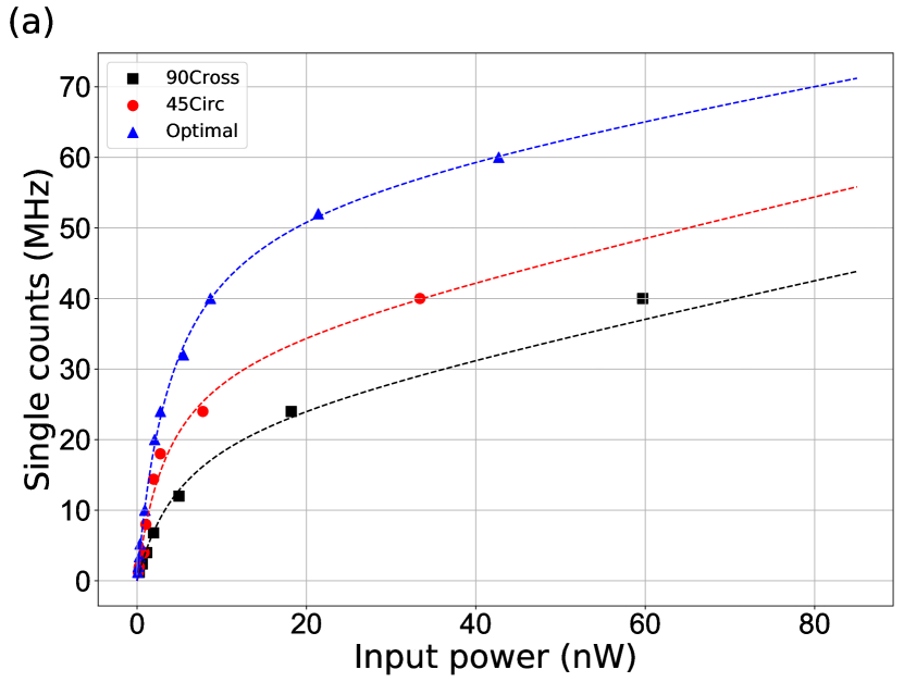
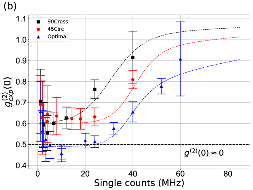
Figure 4: (a) Single-photon count rate $\Gamma$ behind the first lens as a function of the input laser power for the three polarization configurations 90Cross (squares), 45Circ (circles), Optimal (triangles). The dashed curves are fits to Eq. (6) and show good agreement. (b) $g_{exp}^{(2)}(0)$ as a function of the measured single-photon count rate behind the first lens. The dashed curves are the theoretical predictions as described in the text. The increased size of the error bars at higher power is because the $g_{exp}^{(2)}(\tau)$ dip becomes small.

The data in Fig. 4(a) shows the interplay between single-photon light scattered from the QD and leaked coherent laser light. We observe a linear slope for high input power, which corresponds to laser light that leaks through the output polarizer. In Fig. 4(a) we fit the single photon rate, $\Gamma$, using the formula (snijders_fiber-coupled_2018, )

$$\left(x+\left\langle n^{coh}\right\rangle\right)\gamma_{\perp}=\text{$\Gamma$}\frac{\frac{P}{P_{0}}}{1+\frac{P}{P_{0}}}+bP.$$ (6)

Here, $b$ is the fraction of leaked laser light, $P_{0}$ is the saturation power of the QD, and $\Gamma$ is the experimentally obtained single photon rate of the QD. We find for the optimal condition $P_{0}\approx 3\,$nW, $\Gamma\approx 40\,$MHz, and $b\approx 0.5\,$MHz nW^-1. This single photon rate is $25\,$% of the maximal output through one of the mirrors, based on the QD lifetime, $\gamma_{\perp}/2\approx 160\,$MHz. Calculating $g^{(2)}(0)$ using Eq. (5) gives the predictions shown by the dashed curves in Fig. 4(b). For these predictions, we use $\gamma_{\perp}=$ $320\,$MHz in order to obtain the mean photon number $x$. Now, considering the detector response, we estimate $\xi_{90}=0.05$ in Eq. (5) for the 90Cross configuration, which allows us to derive $\xi_{45}=1.6\times\xi_{90}=0.10$ and $\xi_{opt}=3\times\xi_{90}=0.15$ using the data shown in Fig. 3. Here, $\xi$ corresponds to the single-photon brightness as a result of the polarization projection. We see that our theory is in good agreement with the experimental data in Fig. 4(b).

In principle, if the output polarizer could block all residual laser light, a perfectly pure single-photon source is expected. In this case, the brightness of the single-photon source is determined by the polarization change that the QD-scattered single photons experience. At high power, close to QD saturation, the QD also emits non-resonant light, but its effect on the purity is limited in practice compared to the effect of leaked laser light (matthiesen_subnatural_2012, ).

IV conclusion

In conclusion, we have proposed a polarized semi-classical cavity-QED model, and confirmed its accuracy by comparison to experimental data of a QD micro-cavity system. We have shown that this model enables prediction and optimization of the brightness and purity of QD-based single-photon sources, where we have obtained a $3\times$ higher brightness compared to traditional cross-polarization conditions. The model can also be used to optimize pulsed single-photon sources by integrating over the broadened spectrum of the exciting laser.

Appendix A Intuitive derivation of the semi-classical model

Here we show an alternative, intuitive, derivation of Eq. (1) in the main text. We consider two equal mirrors with reflection coefficient $r$ and transmission coefficient $t$ at a distance $L$, like a Fabry-Pérot resonator. The round-trip phase $\phi_{0}$ in the electric field propagation term, written in terms of the wavelength $\lambda_{0}$, refractive index $n$ and length $L$ of the cavity, is:

$$\phi_{0}=\frac{2\pi}{\lambda_{0}}n\left(2L\right)=\frac{4\pi nL}{c}f,$$ (7)

where $c$ is the speed of light and $f$ the frequency of the laser. Since the laser frequency will be scanned across the resonance frequency $f_{c}$ of the Fabry-Pérot cavity, it is convenient to write the phase shift in terms of the relative frequency:

$$\phi=\frac{4\pi nL}{c}\left(f-f_{c}\right).$$ (8)

Further, we assume that there is dispersion and loss in the cavity. We quantify loss of the cavity by single pass amplitude loss $a_{0}$. The QD transition is described by a harmonic oscillator. In the rotating wave approximation, a driven damped harmonic oscillator has a frequency-dependent response similar to a complex Lorentzian. Including cavity loss $a_{0}$, QD loss $a_{QD}$ and Lorentzian dispersion, we obtain a field change in half a round trip of

$$\exp\left(-a+i\frac{\phi}{2}\right),\;\;\;\;\text{where }a\equiv a_{0}+\frac{a_{QD}}{1-i\Delta^{{}^{\prime}}}.$$ (9)

Here, $\Delta^{{}^{\prime}}=\left(f-f_{QD}\right)/\gamma_{\perp}$ with the resonance frequency of the QD $f_{QD}$. By summing over all possible round trips, the total transmission amplitude is

$$\begin{array}[]{c}t_{tot}=tt\exp\left(-a+i\phi/2\right)\left[\sum_{n=0}^{\infty}\left(r^{2}\exp\left(-2a+i\phi\right)\right)^{n}\right]\end{array}$$ (10)

which becomes

$$t_{tot}=\frac{t^{2}\exp\left(-a+i\phi/2\right)}{1-r^{2}\exp\left(-2a+i\phi\right)}.$$ (11)

This formula can be written in a form similar to the semi-classical model by considering $R\sim 1$, small phase changes in the cavity $\phi\ll 1$, in combination with $a_{QD}\ll 1$. This allows us to use a Taylor expansion of the exponentials in Eq. (11). By including all first-order contributions and a few second-order contributions, we write the complex transmission amplitude as

$$t_{tot}\approx\eta_{out}\frac{1}{1-2i\Delta+\frac{2C}{1-i\Delta^{{}^{\prime}}}},$$ (12)

with the out-coupling efficiency

$$\eta_{out}=\frac{1}{\sqrt{1+2a_{0}\left(\frac{1+R}{1-R}\right)}}.$$ (13)

In Appendix B, we show how to derive Eq. (12) and explain that the added higher order Taylor terms to write the final formula in a compact form, are negligible. The out-coupling efficiency $\eta_{out}$ gives the probability that a photon leaves the cavity through one of the mirrors. In Eq. (12), $\Delta$ is the normalized laser-cavity detuning and $\Delta^{\prime}$ is the normalized detuning with respect to the QD transition.

Appendix B Detailed derivation of equation 12

To derive Eq. (12) from Eq. (11), we switch to transmission (intensity) instead of the transmission amplitude (electric field). This has the advantage that the imaginary parts disappear and we get a better understanding of each term in the expansion. Using $1-R=t^{2}=1-r^{2}$, we obtain from Eq. (11)

$$T_{tot}=\frac{\left(1-R\right)^{2}\exp(-2z)}{1+R^{2}\exp(-4z)-2R\exp\left(-2z\right)\cos\left(-2x_{1}+\phi\right)},$$ (14)

with $z=a_{0}+a_{QD}\frac{1}{1+\left(\Delta^{{}^{\prime}}\right)^{2}}$ and $x_{1}=a_{QD}\frac{\Delta^{{}^{\prime}}}{1+\left(\Delta^{{}^{\prime}}\right)^{2}}$. Now we use the following approximations: first, we consider small phase changes $\phi\ll 1$. This, in combination with $a_{QD}\ll 1$, allows us to approximate the cosine term as $\cos\left(-2x_{1}+\phi\right)\approx 1-\frac{\left(-2x_{1}+\phi\right)^{2}}{2}.$ Trying to put the equation in a Lorentzian form gives

$$T_{tot}\approx\frac{1}{1+p_{0}+\left(\frac{-2x_{1}+\phi}{p_{1}}\right)^{2}},$$ (15)

where $p_{1}=$$\frac{1-R}{\sqrt{R}}$ is related to the finesse of an ideal Fabry-Pérot cavity ${F}=\frac{\pi\sqrt{R}}{1-R}$ and $p_{0}$ contains a contribution of loss due to the cavity and the QD. We neglect $x_{1}^{2}$ in Eq. (15) and find

$$T_{tot}\approx\frac{1}{1+p_{0}+\left(\frac{\phi}{p_{1}}\right)^{2}-4\frac{x_{1}\phi}{p_{1}^{2}}}.$$ (16)

After Taylor expanding $p_{0}$ up to second order in $z$ we simplify the analysis by splitting both loss terms and write $p_{0}=p_{c}+p_{QD}$ with

$$p_{c}=2a_{0}\left(\frac{1+R}{1-R}\right),$$ (17)

$$p_{QD}=2\frac{1}{1+\left(\Delta^{{}^{\prime}}\right)^{2}}\left(a_{QD}+a_{QD}^{2}\right)\left(\frac{1+R}{1-R}\right).$$ (18)

For the cavity, we take $p_{c}$ up to first order in $a_{0}$ and $p_{QD}$ up to second order in $a_{QD}$. This choice is made to enable agreement with Eq. (1). With this we can write Eq. (16) as

$$T_{tot}\approx\frac{1}{1+p_{c}}\frac{1}{1+\frac{p_{QD}}{1+p_{c}}+\frac{\phi^{2}}{p_{1}^{2}(1+p_{c})}-4\frac{x_{1}\phi}{p_{1}^{2}\left(1+p_{c}\right)}}.$$ (19)

With the substitutions

$$\kappa=\frac{c(1-R)}{2\pi nL\sqrt{R}}\sqrt{1+p_{c}},$$ (20)

$$\Delta=\frac{f-f_{c}}{\kappa}=\frac{1}{2\pi}\phi{F},\,\mathrm{and}$$ (21)

$$C=a_{QD}\frac{\sqrt{R}}{1-R}\frac{1}{\sqrt{1+p_{c}}}$$ (22)

we find for the total transmission

$$T_{tot}\approx\frac{1}{1+p_{c}}\frac{1}{1+4\Delta^{2}-8C\frac{\Delta\Delta^{{}^{\prime}}}{1+\left(\Delta^{{}^{\prime}}\right)^{2}}+\frac{2C}{1+\left(\Delta^{{}^{\prime}}\right)^{2}}\left(2+2C\right)},$$ (23)

where $\frac{p_{QD}}{1+p_{c}}\sim\frac{2C}{1+\left(\Delta^{{}^{\prime}}\right)^{2}}\left(2+2C\right)$ assuming that $R\sim 1$. Now we go back to the complex transmission amplitude $t_{tot}=\sqrt{T_{tot}}$ of Eq. (23) and arrive at Eq. (12). In order to confirm that the above approximations are valid we compare Eq. (14) to the semi-classical model of Eq. (12) in Fig. 5 for a micro-cavity with center wavelength $\lambda=930\,$$nm$, $n=2$, $R=0.95$, $a_{0}=0.01$, $a_{QD}=0.03$, and $L=0.1\,$$\mu$m. We see that both models agree very well, suggesting that our approximations are valid. The slight deviations in the peak height is due to the assumption that the cavity absorption $a_{0}$ is treated as a first order effect in the semi-classical model.

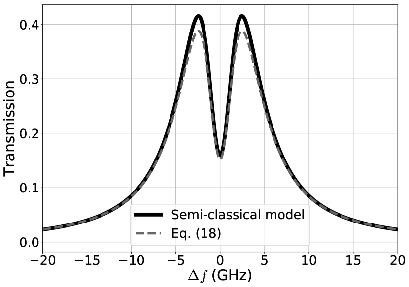
Figure 5: Comparison of the semi-classical model of Eq. (12) to the exact classical model of the lossy Fabry-Pérot cavity in Eq. (14) for realistic parameters. The deviation between the dashed and solid line is because in the semi-classical model only the first order effect of absorption is taken into account.

Appendix C Comparison between the extended semi-classical and the quantum master model

Here we investigate the limit of our semi-classical model by increasing the power to higher mean photon numbers. The mean photon number is changed for the optimal polarization condition (Fig. (3)) and the condition where the output polarizer is removed. We see in Fig. (6) that our results are similar up to $\langle n\rangle=0.01,$ for higher power the results deviate due to saturation of the QD transitions.

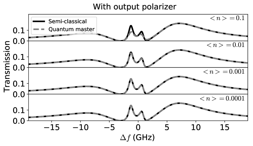
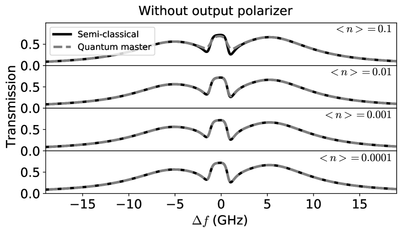
Figure 6: Transmission spectra for the experimental case discussed in Figs. 3 and 4 of a neutral quantum dot with fine-structure splitting for the optimal polarization condition (with and without output polarizer) at different input power. Only at high input power ($\langle n\rangle=0.1$), our extended semi-classical model deviates a bit from the quantum master equation simulations.

References

- (1) Grange, T., Hornecker, G., Hunger, D., Poizat, J.-P., Gérard, J.-M., Senellart, P. & Auffèves, A. Cavity-Funneled Generation of Indistinguishable Single Photons from Strongly Dissipative Quantum Emitters. Physical Review Letters 114, 193601 (2015).
- (2) Somaschi, N., Giesz, V., De Santis, L., Loredo, J. C., Almeida, M. P., Hornecker, G., Portalupi, S. L., Grange, T., Antón, C., Demory, J., Gómez, C., Sagnes, I., Lanzillotti-Kimura, N. D., Lemaítre, A., Auffeves, A., White, A. G., Lanco, L. & Senellart, P. Near-optimal single-photon sources in the solid state. Nature Photonics 10, 340 (2016).
- (3) Ding, X., He, Y., Duan, Z.-C., Gregersen, N., Chen, M.-C., Unsleber, S., Maier, S., Schneider, C., Kamp, M., Höfling, S., Lu, C.-Y. & Pan, J.-W. On-Demand Single Photons with High Extraction Efficiency and Near-Unity Indistinguishability from a Resonantly Driven Quantum Dot in a Micropillar. Physical Review Letters 116, 020401 (2016).
- (4) Wang, H., He, Y.-M., Chung, T.-H., Hu, H., Yu, Y., Chen, S., Ding, X., Chen, M.-C., Qin, J., Yang, X., Liu, R.-Z., Duan, Z.-C., Li, J.-P., Gerhardt, S., Winkler, K., Jurkat, J., Wang, L.-J., Gregersen, N., Huo, Y.-H., Dai, Q., Yu, S., Höfling, S., Lu, C.-Y. & Pan, J.-W. Towards optimal single-photon sources from polarized microcavities. Nature Photonics 13, 770 (2019).
- (5) Imamoglu, A., Schmidt, H., Woods, G. & Deutsch, M. Strongly Interacting Photons in a Nonlinear Cavity. Physical Review Letters 79, 1467 (1997).
- (6) Kimble, H. J. The quantum internet. Nature 453, 1023 (2008).
- (7) Armen, M. a. & Mabuchi, H. Low-lying bifurcations in cavity quantum electrodynamics. Physical Review A 73, 063801 (2006).
- (8) Waks, E. & Vuckovic, J. Dipole Induced Transparency in Drop-Filter Cavity-Waveguide Systems. Physical Review Letters 96, 153601 (2006).
- (9) Auffèves-Garnier, A., Simon, C., Gérard, J.-M. & Poizat, J.-P. Giant optical nonlinearity induced by a single two-level system interacting with a cavity in the Purcell regime. Physical Review A 75, 053823 (2007).
- (10) Loo, V., Arnold, C., Gazzano, O., Lemaitre, A., Sagnes, I., Krebs, O., Voisin, P., Senellart, P. & Lanco, L. Optical nonlinearity with few-photon pulses using a quantum dot-pillar cavity device. Physical Review Letters 109, 166806 (2012).
- (11) Majumdar, A., Englund, D., Bajcsy, M. & Vučković, J. Nonlinear temporal dynamics of a strongly coupled quantum-dot–cavity system. Physical Review A 85, 033802 (2012).
- (12) Hu, C. Y. & Rarity, J. G. Extended linear regime of cavity-QED enhanced optical circular birefringence induced by a charged quantum dot. Physical Review B 91, 075304 (2015).
- (13) Bakker, M. P., Barve, A. V., Ruytenberg, T., Löffler, W., Coldren, L. A., Bouwmeester, D. & Van Exter, M. P. Polarization degenerate solid-state cavity quantum electrodynamics. Physical Review B 91, 115319 (2015).
- (14) All frequencies and rates here are ordinary and measured in hertz.
- (15) Bonato, C., Ding, D., Gudat, J., Thon, S., Kim, H., Petroff, P. M., van Exter, M. P. & Bouwmeester, D. Tuning micropillar cavity birefringence by laser induced surface defects. Applied Physics Letters 95, 251104 (2009).
- (16) Frey, J. A., Snijders, H. J., Norman, J., Gossard, A. C., Bowers, J. E., Löffler, W. & Bouwmeester, D. Electro-optic polarization tuning of microcavities with a single quantum dot. Optics Letters 43, 4280 (2018).
- (17) Antón, C., Hilaire, P., Kessler, C. A., Demory, J., Gómez, C., Lemaître, A., Sagnes, I., Lanzillotti-Kimura, N. D., Krebs, O., Somaschi, N., Senellart, P. & Lanco, L. Tomography of the optical polarization rotation induced by a single quantum dot in a cavity. Optica 4, 1326 (2017).
- (18) He, Y.-M., Wang, H., Gerhardt, S., Winkler, K., Jurkat, J., Yu, Y., Chen, M.-C., Ding, X., Chen, S., Qian, J., Li, J.-P., Wang, L.-J., Huo, Y.-H., Yu, S., Lu, C.-Y. & Pan, J.-W. Polarized indistinguishable single photons from a quantum dot in an elliptical micropillar. arXiv:1809.10992 (2018).
- (19) Snijders, H. & Löffler, W. An extended semi-classical model for polarized quantum dot cavity-QED and application to single photon sources (2018). Https://doi.org/10.5281/zenodo.3476660.
- (20) Bayer, M., Ortner, G., Stern, O., Kuther, A., Gorbunov, A. A., Forchel, A., Hawrylak, P., Fafard, S., Hinzer, K., Reinecke, T. L., Walck, S. N., Reithmaier, J. P., Klopf, F. & Schäfer, F. Fine structure of neutral and charged excitons in self-assembled In(Ga)As/(Al)GaAs quantum dots. Physical Review B 65, 195315 (2002).
- (21) Warburton, R. J. Single spins in self-assembled quantum dots. Nature Materials 12, 483 (2013).
- (22) Fowles, G. Introduction to Modern Optics (Dover Publications, New York, 1989), 2nd edn.
- (23) Johansson, J., Nation, P. & Nori, F. QuTiP: An open-source Python framework for the dynamics of open quantum systems. Computer Physics Communications 183, 1760 (2012).
- (24) Johansson, J. R., Nation, P. D. & Nori, F. QuTiP 2: A Python framework for the dynamics of open quantum systems. Computer Physics Communications 184, 1234 (2013).
- (25) Snijders, H., Frey, J. A., Norman, J., Bakker, M. P., Langman, E. C., Gossard, A., Bowers, J. E., Van Exter, M. P., Bouwmeester, D. & Löffler, W. Purification of a single-photon nonlinearity. Nature Communications 7, 12578 (2016).
- (26) Proux, R., Maragkou, M., Baudin, E., Voisin, C., Roussignol, P. & Diederichs, C. Measuring the Photon Coalescence Time Window in the Continuous-Wave Regime for Resonantly Driven Semiconductor Quantum Dots. Physical Review Letters 114, 067401 (2015).
- (27) Snijders, H., Frey, J. A., Norman, J., Post, V. P., Gossard, A. C., Bowers, J. E., van Exter, M. P., Löffler, W. & Bouwmeester, D. Fiber-Coupled Cavity-QED Source of Identical Single Photons. Physical Review Applied 9, 031002 (2018).
- (28) Matthiesen, C., Vamivakas, A. N. & Atatüre, M. Subnatural Linewidth Single Photons from a Quantum Dot. Physical Review Letters 108, 093602 (2012).