Fluctuating shapes of the fireballs in heavy-ion collisions

Abstract

We argue that energy and momentum deposition from hard partons into quark-gluon plasma induces an important contribution to the final state hadron anisotropies. We also advocate a novel method of Event Shape Sorting which allow to analyse the azimuthal anisotropies of the fireball dynamics in more detail. A use of the method in femtoscopy is demonstrated.

1 Motivation

In ultrarelativistic heavy-ion collisions, numbers of produced hadrons are so large that empirical distributions of their azimuthal angles can reasonably be constructed. Large anisotropies exist in those distributions. Moreover, these anisotropies are different in every collision event. The usual paradigm is that these anisotropies result from the response of the hot matter to the inhomogeneities within its initial state. This response is determined by features like the Equation of State (EoS) or the transport coefficients. Those we would like to extract from the response. The caveat is that the initial conditions are largely unknown and not directly accessible through a measurement.

In this overview talk we bring up two issues which concern this standard interpretation of the fireball evolution.

In the first part we argue that the final state anisotropies can also be produced by the momentum and energy deposition from hard partons traversing the deconfined matter Schulc:2014jma ; Tachibana:2014lja . This source of anisotropy, which is not present in the initial conditions, is relevant in collisions at the LHC energy.

Since usually many events are summed up in order to obtain better statistic, some anisotropies may be averaged out in such summations. The method of Event Shape Sorting Kopecna:2015fwa , introduced in the second part of this talk, helps to organise the event averaging in such a way that the final state anisotropies survive better. Such events with a richer structure of the azimuthal angle distribution might better help to reconstruct the properties of the hot matter from the response to initial inhomogeneities.

2 Bulk anisotropic flow from hard partons

In nuclear collisions at LHC energies, many hard partons are produced in the initial interactions of the incoming partons from the two nuclei. The share of energy out of all energy deposited in a collision is larger than at RHIC or SPS. Shortly after they are produced, the deconfined medium fills the space around them. Hence, they evolve in this quark-gluon plasma (QGP) and loose energy and momentum in favour of the bulk. Depending on the total energy of the parton and the size of the energy loss, this process spans over some time. During this time the deposited momentum and energy lead to production of collective mechanical effects in the QGP: wakes and Mach cones Satarov:2005mv ; CasalderreySolana:2004qm ; Neufeld:2008fi . Most important for us are the streams in the wakes which carry the momentum of the original hard parton Schulc:2013kra .

The resulting flow anisotropies are different in each event. A naive expectation would be that they are averaged out if many events are summed up, because hard partons are produced isotropically in the transverse plane. It turns out that this is not true. They are correlated with the geometry of a non-central collision. Two streams are more likely to meet each other if they are produced in the direction perpendicular to the reaction plane. Then they (partially) cancel each others momentum. Thus more bulk flow is induced in the direction of the impact parameter. This is a positive contribution to the elliptic flow due to pressure gradient anisotropy in the initial state.

In order to study this effect we implemented source terms in 3D ideal hydrodynamic simulation Schulc:2014jma . The used Equation of State was parametrised from lattice QCD results Huovinen:2009yb . Initial conditions were smooth, calculated with optical Glauber model and the rapidity profile of the fluid was flat. Hard partons were introduced into this environment at the beginning of its evolution. They are produced as back-to-back pairs (due to transverse momentum conservation) with fluctuating number of pairs and power-law distribution of the $p_{t}$’s.

Figure 1

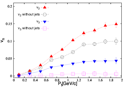
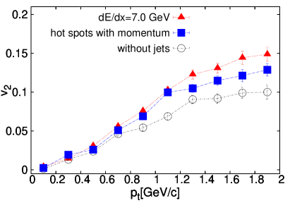
Figure 1: Anisotropic flow coefficients generated by momentum deposition from hard partons in centrality class 30–40%. Left: $v_{2}$ and $v_{3}$ from simulations with momentum deposition and without it, only with smooth initial conditions (“without jets”). Right: The curve with squares shows results from a simulation with no momentum deposition from hard partons, but with the same amount of momentum and energy anisotropies superimposed on the smooth initial energy density profile in form of hot spots.

shows the effect of the momentum depostion. In non-central collisions the elliptic flow is increased by about 50% in comparison to simulations with smooth initial conditions. Since there is no triangular anisotropy present in the initial conditions, the third-order coefficient $v_{3}$ is entirely due to energy and momentum deposition from hard partons.

We have also investigated if the effect can be fully included into the initial conditions. To this end, we superimposed on the smooth initial energy density profile a number of “hot spots” which carried exactly the energy and momentum of the hard partons. The resulting $v_{2}$ (Fig. 1 right) falls short of the elliptic anisotropy due to hard partons.

We conclude that momentum deposition from hard partons during the evolution of the fireball is an important ingredient which must not be omitted in simulations which aim at extracting matter properties via a comparison with experimental data Tachibana:2017syd .

3 Event Shape Sorting

Anisotropies of the final state distributions of hadrons are to a large extent characteristic for each collision event. In a single event, it is also possible to measure the anisotropies which disappear in event averaging, e.g. by making use of correlation between hadrons. Nevertheless, the question remains if one can select events for the analysis in such a way, that at least a part of the characteristics is not washed away in the sum of many events.

Indeed, such a technique has been suggested under the name Event Shape Engineering (ESE) Schukraft:2012ah . When using ESE, first an observable is defined according to the which a selection of events will be done. That observable is measured in every event. Events with the value of the observable within a specified interval are selected into one class.

For example, one determines $|q_{2}|=|\sum_{i=1}^{M}e^{2i\phi_{i}}|/\sqrt{M}$, where $M$ is the multiplicity in the acceptance interval and $\phi_{i}$ is the measured azimuthal angle of the $i$-th recorded hadron. The events with large $q_{2}$ are treated separately from small $q_{2}$. ESE is able to separate events effectively and in a well controlled way.

On the other hand, the choice of the sorting observable (i.e. $q_{2}$ in the above example) must be provided by hand. If there exists some hidden structure according to which the events differ in their shapes, it might remain unobserved in ESE. In other words, ESE reveals the differences between events, provided that you tell at the beginning how the differences look like.

In order to overcome this feature, we proposed a different method recently Kopecna:2015fwa ; Lehmann:2007pv , under the name Event Shape Sorting (ESS). In ESS, no observable is pre-defined, according to which the selection of events is made. Instead, the algorithm itself re-orders the analysed events in such a way, that events with similar shapes end up close to each other.

Technically, it works with the histograms in azimuthal angles for individual events. The totality of events is divided into several percentiles, typically deciles. We shall refer to these percentiles as to event bins and number them from 1 to 10. Then, Bayesian probability is determined for each event that it belongs to a given event bin. This probability is determined for every event bin. Based on these probabilities the events are then re-arranged in such a way, that each event comes to the place where it currently fits best. The procedure is iterated until the order of events stops changing in the next iteration.

3.1 Results from Event Shape Sorting

We present here results which we obtained with event sets simulated by two different event generators. The first set is composed of $1.5\times 10^{5}$ events generated by DRAGON Tomasik:2008fq . This is an MC generator of final state hadrons according to the Blast-Wave model with included resonances. We included anisotropies of second and third order in both shape and flow profile Cimerman:2017lmm .

The other two sets of events are provided by AMPT Lin:2004en , which has been run for Au+Au collisions at impact parameter 7-10 fm at both $\sqrt{s_{NN}}=200$ GeV (AMPT-RHIC) and $\sqrt{s_{NN}}=2760$ GeV (AMPT-LHC). There are $10^{4}$ events in each of the AMPT sets.

As a first example of how the method works we compare the sorting with the two main components of the flow anisotropy in the game: $v_{2}$ and $v_{3}$. Note that before comparing the shapes of the events we have rotated them in such a way that all second-order event planes point in the same direction. In order to be able to follow a change of the third-order event plane direction, we allow also for negative values of $v_{3}$. They would turn positive if the event plane would be shifted by $\pi/3$.

In Figure 2 it is demonstrated how the dominance of the elliptic flow

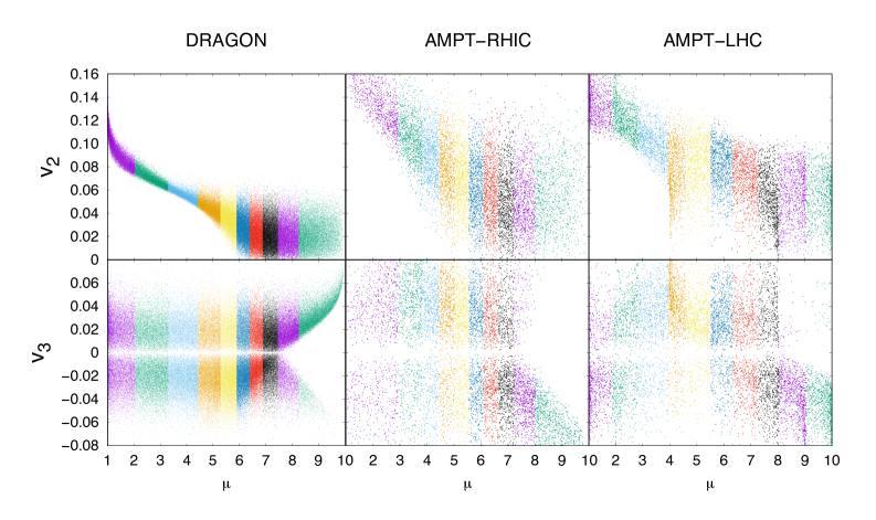
Figure 2: Correlation of the sorting variable $\mu$ with $v_{2}$ (upper row) and $v_{3}$ (lower row) for all events from the sets generated by DRAGON (left column), AMPT for RHIC (middle) and AMPT for the LHC (right). The variable $\mu$ is the one according to which value the events are ordered. Different event bins are indicated with different colours; each dot corresponds to one event.

shows up in the sorting of all events. This is best seen in the set generated by DRAGON. The event bins at low sorting variable $\mu$ are determined by large elliptic flow. On the other hand, those event bins at high $\mu$’s have all elliptic anisotropy within roughly the same interval, but they differ by the triangular anisotropy. Qualitatively, similar features are present in the AMPT events, although the magnitude of the anisotropies is somewhat higher. Small statistics prevents drawing more precise conclusions from the AMPT simulations.

We have also determined the HBT correlation radii, which appear in the Gaussian parametrisation of the correlation function

$$C(q,K)-1=\exp\left(-R_{o}^{2}(K)q_{o}^{2}-R_{s}^{2}(K)q_{s}^{2}-R_{l}^{2}(K)q_{l}^{2}\right)\,,$$ (1)

where $K$ is average pair momentum and the $q$’s are components of the momentum difference (and cross-terms vanish in symmetric systems at midrapidity). Let us note that they measure the sizes of homogeneity regions, i.e. those parts of the fireball which produce hadrons with specified momentum. Due to flow gradients, in an expanding fireball the homogeneity regions are smaller than the whole fireball. The correlation radii depend on the azimuthal angle, because pions flying in different directions come from different homogeneity regions.

This is shown in Figure 3.

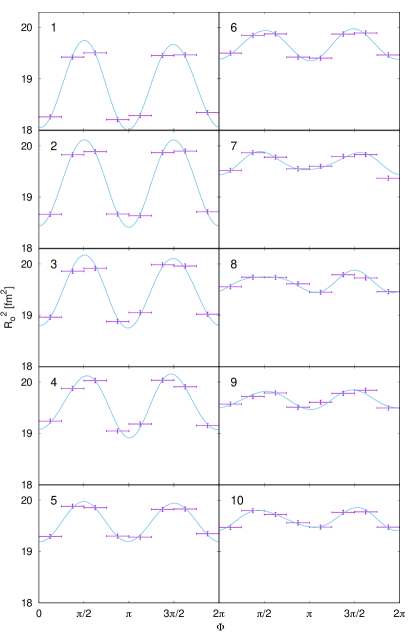
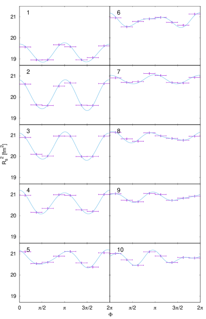
Figure 3: Dependences of the correlation radii on the azimuthal angle, as they result from simulations with DRAGON. Plotted are $R_{o}^{2}$ (left) and $R_{s}^{2}$ (right) and different panels show different event bins, as indicated by event bin number in each panel.

We can see, in accord with Figure 2, that at lower $\mu^{\prime}s$ there are mainly second-order oscillations. The third order Fourier component of the azimuthal dependence is seen in event bins with larger $\mu$, also in accord with Figure 2. We stress here, that a measurement of the second and third order anisotropy in one curve is only possible with the help of ESS. They are not seen both together if all events have been just aligned with respect to either second or third-order event plane and summed up.

In order to single out the amplitude of the anisotropies from the overall size of the radii, the terms can be scaled by the zeroth-order term

$$R_{i}^{2}=R_{i,0}^{2}+\sum_{j=1}^{\infty}R_{i,j}^{2}\cos\left(n(\phi-\phi_{n})\right)=R_{i,0}^{2}\left(1+\sum_{j=1}^{\infty}\frac{R_{i,j}^{2}}{R_{i,0}^{2}}\cos\left(n(\phi-\phi_{n})\right)\right)\,.$$ (2)

The scaled amplitudes are plotted in Figure 4. Those from DRAGON simulations actually parametrize the curves seen in Figure 3.

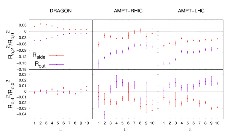
Figure 4: Scaled oscillation amplitudes for $R_{o}^{2}$ and $R_{s}^{2}$ in the second order (upper row) and the third order (lower row) for different event bins (they are plotted as functions of the event bin number). Simulations by DRAGON (left), AMPT for RHIC (middle) and AMPT for the LHC (right).

The second-order amplitude for DRAGON events behaves similarly as $v_{2}$ in Figure 2, while the sizes of the third-order amplitude are small and basically consistent with 0. Larger amplitudes at both orders are seen in the AMPT events.

4 Conclusions

Event Shape Sorting provides new insights in the final state distribution of hadrons, since it makes it possible to observe both second and third-order oscillations of hadron distributions and correlation radii together at the same time. This should allow for a more differential comparison of theory to data.

We have also argued, that in collisions at the LHC, it is important to add to hydrodynamic modelling the momentum deposition from hard partons into the bulk medium.

Acknowledgment

Supported by the grant 17-04505S of the Czech Science Foundation (GAČR). BT also acknowledges support by VEGA 1/0348/18 (Slovakia).

References

- (1) M. Schulc and B. Tomášik, Phys. Rev. C 90 064910 (2014)
- (2) Y. Tachibana and T. Hirano, Phys. Rev. C 90 021902 (2014)
- (3) R. Kopečná and B. Tomášik, Eur. Phys. J. A 52 115 (2016)
- (4) L. M. Satarov, H. Stöcker and I. N. Mishustin, Phys. Lett. B 627 64 (2005)
- (5) J. Casalderrey-Solana, E. V. Shuryak and D. Teaney, J. Phys. Conf. Ser. 27 22 (2005)
- (6) R. B. Neufeld, B. Müller and J. Ruppert, Phys. Rev. C 78 041901 (2008)
- (7) M. Schulc and B. Tomášik, J. Phys. G 40 125104 (2013)
- (8) P. Huovinen and P. Petreczky, Nucl. Phys. A 837 26 (2010)
- (9) Y. Tachibana, N. B. Chang and G. Y. Qin, Phys. Rev. C 95 044909 (2017)
- (10) J. Schukraft, A. Timmins and S. A. Voloshin, Phys. Lett. B 719 394 (2013)
- (11) S. Lehmann, A. D. Jackson and B. E. Lautrup, Scientometrics 76 369 (2008)
- (12) B. Tomášik, Comput. Phys. Commun. 180, 1642 (2009) and ibid 207 545 (2016)
- (13) J. Cimerman, B. Tomášik, M. Csanád and S. Lökös, Eur. Phys. J. A 53 161 (2017)
- (14) Z. W. Lin, C. M. Ko, B. A. Li, B. Zhang and S. Pal, Phys. Rev. C 72, 064901 (2005)