Hessian Riemannian gradient flows in convex programming

Abstract Motivated by a constrained minimization problem, it is studied the gradient flows with respect to Hessian Riemannian metrics induced by convex functions of Legendre type. The first result characterizes Hessian Riemannian structures on convex sets as those metrics that have a specific integration property with respect to variational inequalities, giving a new motivation for the introduction of Bregman-type distances. Then, the general evolution problem is introduced and a differential inclusion reformulation is given. A general existence result is proved and global convergence is established under quasi-convexity conditions, with interesting refinements in the case of convex minimization. Some explicit examples of these gradient flows are discussed. Dual trajectories are identified and sufficient conditions for dual convergence are examined for a convex program with positivity and equality constraints. Some convergence rate results are established. In the case of a linear objective function, several optimality characterizations of the orbits are given: optimal path of viscosity methods, continuous-time model of Bregman-type proximal algorithms, geodesics for some adequate metrics and projections of $\dot{q}$-trajectories of some Lagrange equations and completely integrable Hamiltonian systems.

Keywords Gradient flow, Hessian Riemannian metric, Legendre type convex function, existence, global convergence, Bregman distance, Liapounov functional, quasi-convex minimization, convex and linear programming, Legendre transform coordinates, Lagrange and Hamilton equations.

AMS classification: 34G20, 34A12, 34D05, 90C25.

1 Introduction

The aim of this paper is to study the existence, global convergence and geometric properties of gradient flows with respect to a specific class of Hessian Riemannian metrics on convex sets. Our work is indeed deeply related to the constrained minimization problem

$$\min\{f(x)\mid x\in\overline{C},\;Ax=b\},$$

where $\overline{C}$ is the closure of a nonempty, open and convex subset $C$ of $\mathbb{R}^{n}$, $A$ is a $m<n$ real matrix with $m\leq n$, $b\in\mathbb{R}^{m}$ and $f\in C^{1}(\mathbb{R}^{n})$. A strategy to solve $(P)$ consists in endowing $C$ with a Riemannian structure $(\cdot,\cdot)^{H}$, to restrict it to the relative interior of the feasible set ${{\cal F}}:=C\cap\{x\mid Ax=b\}$, and then to consider the trajectories generated by the steepest descent vector field $-\nabla_{{}_{H}}f_{|_{{{\cal F}}}}$. This leads to the initial value problem

$$(H\mbox{-}SD)\qquad\dot{x}(t)+\nabla_{{}_{H}}f_{|_{{{\cal F}}}}(x(t))=0,\>x(0)\in{{\cal F}},$$

where $(H\mbox{-}SD)$ stands for $H$-steepest descent. We focus on those metrics that are induced by the Hessian $H=\nabla^{2}h$ of a Legendre type convex function $h$ defined on $C$ (cf. Def. 3.1).

The use of Riemannian methods in optimization has increased recently: in relation with Karmarkar algorithm and linear programming see Karmarkar [29], Bayer-Lagarias [5]; for continuous-time models of proximal type algorithms and related topics see Iusem-Svaiter-Da Cruz [27], Bolte-Teboulle [6]. For a systematic dynamical system approach to constrained optimization based on double bracket flows, see Brockett [8, 9], the monograph of Helmke-Moore [22] and the references therein. On the other hand, the structure of $(H\mbox{-}SD)$ is also at the heart of some important problems in applied mathematics. For connections with population dynamics and game theory see Hofbauer-Sygmund [25], Akin [1], Attouch-Teboulle [3]. We will see that $(H\mbox{-}SD)$ can be reformulated as the differential inclusion $\frac{d}{dt}\nabla h(x(t))+\nabla f(x(t))\in{\rm Im}\>A^{T},\>x(t)\in{{\cal F}},$ which is formally similar to some evolution problems in infinite dimensional spaces arising in thermodynamical systems, see for instance Kenmochi-Pawlow [30] and references therein.

A classical approach in the asymptotic analysis of dynamical systems consists in exhibiting attractors of the orbits by using Liapounov functionals. Our choice of Hessian Riemannian metrics is based on this idea. In fact, we consider first the important case where $f$ is convex, a condition that permits us to reformulate $(P)$ as a variational inequality problem: $\mbox{find }a\in\overline{{{\cal F}}}\mbox{ such that }(\nabla_{{}_{H}}f_{|_{{{\cal F}}}}(x),x-a)^{H}_{x}\geq 0\>\mbox{ for all }x\mbox{ in }{{\cal F}}.$ In order to identify a suitable Liapounov functional, this variational problem is met through the following integration problem: find the metrics $(\cdot,\cdot)^{H}$ for which the vector fields $V^{a}:{{\cal F}}\to\mathbb{R}^{n}$, $a\in{{\cal F}}$, defined by $V^{a}(x)=x-a,$ are $(\cdot,\cdot)^{H}$-gradient vector fields. Our first result (cf. Theorem 3.1) establishes that such metrics are given by the Hessian of strictly convex functions, and in that case the vector fields $V^{a}$ appear as gradients with respect to the second variable of some distance-like functions that are called $D$-functions. Indeed, if $(\cdot,\cdot)^{H}$ is induced by the Hessian $H=\nabla^{2}h$ of $h:{{\cal F}}\mapsto\mathbb{R}$, we have for all $a,x$ in ${{\cal F}}$: $\nabla_{{}_{H}}D_{h}(a,.)(x)=x-a,\mbox{ where }D_{h}(a,x)=h(a)-h(x)-dh(x)(x-a).$ For another characterization of Hessian metrics, see Duistermaat [17].

Motivated by the previous result and with the aim of solving $(P)$, we are then naturally led to consider Hessian Riemannian metrics that cannot be smoothly extended out of ${{\cal F}}$. Such a requirement is fulfilled by the Hessian of a Legendre (convex) function $h$, whose definition is recalled in section 3. We give then a differential inclusion reformulation of $(H\mbox{-}SD)$, which permits to show that in the case of a linear objective function $f$, the flow of $-\nabla_{{}_{H}}f_{|_{{{\cal F}}}}$ stands at the crossroad of many optimization methods. In fact, following [27], we prove that viscosity methods and Bregman proximal algorithms produce their paths or iterates in the orbit of $(H\mbox{-}SD)$. The $D$-function of $h$ plays an essential role for this. In section 4.4 it is given a systematic method to construct Legendre functions based on barrier functions for convex inequality problems, which is illustrated with some examples; relations to other works are discussed.

Section 4 deals with global existence and convergence properties. After having given a non trivial well-posedness result (cf. Theorem 4.1), we prove in section 4.2 that $f(x(t))\rightarrow\inf_{\overline{{{\cal F}}}}f$ as $t\rightarrow+\infty$ whenever $f$ is convex. A natural problem that arises is the trajectory convergence to a critical point. Since one expects the limit to be a (local) solution to $(P)$, which may belong to the boundary of $C$, the notion of critical point must be understood in the sense of the optimality condition for a local minimizer $a$ of $f$ over $\overline{{{\cal F}}}$:

$$({\cal O})\qquad\nabla f(a)+N_{\overline{{{\cal F}}}}(a)\ni 0,\>a\in\overline{{{\cal F}}},$$

where $N_{\overline{{{\cal F}}}}(a)$ is the normal cone to $\overline{{{\cal F}}}$ at $a$, and $\nabla f$ is the Euclidean gradient of $f$. This involves an asymptotic singular behavior that is rather unusual in the classical theory of dynamical systems, where the critical points are typically supposed to be in the manifold. In section 4.3 we assume that the Legendre type function $h$ is a Bregman function with zone $C$ and prove that under a quasi-convexity assumption on $f$, the trajectory converges to some point $a$ satisfying $({\cal O})$. When $f$ is convex, the preceding result amounts to the convergence of $x(t)$ toward a global minimizer of $f$ over $\overline{{{\cal F}}}$. We also give a variational characterization of the limit and establish an abstract result on the rate of convergence under uniqueness of the solution. We consider in section 4.5 the case of linear programming, for which asymptotic convergence as well as a variational characterization are proved without the Bregman-type condition. Within this framework, we also give some estimates on the convergence rate that are valid for the specific Legendre functions commonly used in practice. In section 4.6, we consider the interesting case of positivity and equality constraints, introducing a dual trajectory $\lambda(t)$ that, under some appropriate conditions, converges to a solution to the dual problem of $(P)$ whenever $f$ is convex, even if primal convergence is not ensured.

Finally, inspired by the seminal work [5], we define in section 5 a change of coordinates called Legendre transform coordinates, which permits to show that the orbits of $(H\mbox{-}SD)$ may be seen as straight lines in a positive cone. This leads to additional geometric interpretations of the flow of $-\nabla_{{}_{H}}f_{|_{{{\cal F}}}}$. On the one hand, the orbits are geodesics with respect to an appropriate metric and, on the other hand, they may be seen as $\dot{q}$-trajectories of some Lagrangian, with consequences in terms of integrable Hamiltonians.

Notations. ${\rm Ker}\>A=\{x\in\mathbb{R}^{n}\;|\;Ax=0\}.$ The orthogonal complement of ${\cal A}_{0}$ is denoted by ${\cal A}_{0}^{\perp}$, and $\langle\cdot,\cdot\rangle$ is the standard Euclidean scalar product of $\mathbb{R}^{n}$. Let us denote by $\mathbb{S}_{++}^{n}$ the cone of real symmetric definite positive matrices. Let $\Omega\subset\mathbb{R}^{n}$ be an open set. If $f:\Omega\to\mathbb{R}$ is differentiable then $\nabla f$ stands for the Euclidean gradient of $f$. If $h:\Omega\mapsto\mathbb{R}$ is twice differentiable then its Euclidean Hessian at $x\in\Omega$ is denoted by $\nabla^{2}h(x)$ and is defined as the endomorphism of $\mathbb{R}^{n}$ whose matrix in canonical coordinates is given by $[\frac{\partial^{2}h(x)}{\partial x_{i}\partial x_{j}}]_{i,j\in\{1,..,n\}}$. Thus, $\forall x\in\Omega$, $d^{2}h(x)=\langle\nabla^{2}h(x)\>\cdot,\cdot\rangle$.

2 Preliminaries

2.1 The minimization problem and optimality conditions

Given a positive integer $m<n$, a full rank matrix $A\in\mathbb{R}^{m\times n}$ and $b\in{\rm Im}\>A$, let us define

$${\cal A}=\{x\in\mathbb{R}^{n}\;|\;Ax=b\}.$$ (1)

Set ${\cal A}_{0}={\cal A}-{\cal A}={\rm Ker}\>A$. Of course, ${\cal A}_{0}^{\perp}={\rm Im}\>A^{T}$ where $A^{T}$ is the transpose of $A$. Let $C$ be a nonempty, open and convex subset of $\mathbb{R}^{n}$, and $f:\mathbb{R}^{n}\to\mathbb{R}$ a ${\cal C}^{1}$ function. Consider the constrained minimization problem

$$\inf\{f(x)\;|\;x\in\overline{C},\;Ax=b\}.$$

The set of optimal solutions of $(P)$ is denoted by $S(P)$. We call $f$ the objective function of $(P)$. The feasible set of $(P)$ is given by $\overline{{{\cal F}}}=\{x\in\mathbb{R}^{n}\;|\;x\in\overline{C},\;Ax=b\}=\overline{C}\cap{\cal A},$ and ${{\cal F}}$ stands for the relative interior of $\overline{{{\cal F}}}$, that is

$${{\cal F}}={\rm ri}\>\overline{{{\cal F}}}=\{x\in\mathbb{R}^{n}\;|\;x\in C,\;Ax=b\}=C\cap{\cal A}.$$ (2)

Throughout this article, we assume that

$${{\cal F}}\neq\emptyset.$$ (3)

It is well known that a necessary condition for $a$ to be locally minimal for $f$ over $\overline{{{\cal F}}}$ is $({\cal O}):\>-\nabla f(a)\in N_{\overline{{{\cal F}}}}(a)$, where $N_{\overline{{{\cal F}}}}(x)=\{\nu\in\mathbb{R}^{n}\;|\;\forall y\in\overline{{{\cal F}}},\;\langle y-x,\nu\rangle\leq 0\}$ is the normal cone to $\overline{{{\cal F}}}$ at $x\in\overline{{{\cal F}}}$ ($N_{\overline{{{\cal F}}}}(x)=\emptyset$ when $x\notin\overline{{{\cal F}}}$); see for instance [37, Theorem 6.12]. By [36, Corollary 23.8.1], $N_{\overline{{{\cal F}}}}(x)=N_{\overline{C}\cap{\cal A}}(x)=N_{\overline{C}}(x)+N_{{\cal A}}(x)=N_{\overline{C}}(x)+{\cal A}_{0}^{\perp},$ for all $x\in\overline{{{\cal F}}}$. Therefore, the necessary optimality condition for $a\in\overline{{{\cal F}}}$ is

$$-\nabla f(a)\in N_{\overline{C}}(a)+{\cal A}_{0}^{\perp}.$$ (4)

If $f$ is convex then this condition is also sufficient for $a\in\overline{{{\cal F}}}$ to be in $S(P)$.

2.2 Riemannian gradient flows on the relative interior of the feasible set

Let $M$ be a smooth manifold. The tangent space to $M$ at $x\in M$ is denoted by $T_{x}M$. If $f:M\mapsto\mathbb{R}$ is a ${\cal C}^{1}$ function then $df(x)$ denotes its differential or tangent map $df(x):T_{x}M\to\mathbb{R}$ at $x\in M$. A ${\cal C}^{k}$ metric on $M$, $k\geq 0$, is a family of scalar products $(\cdot,\cdot)_{x}$ on each $T_{x}M$, $x\in M$, such that $(\cdot,\cdot)_{x}$ depends in a ${\cal C}^{k}$ way on $x$. The couple $M,(\cdot,\cdot)_{x}$ is called a ${\cal C}^{k}$ Riemannian manifold. This structure permits to identify $T_{x}M$ with its dual, i.e. the cotangent space $T_{x}M^{*}$, and thus to define a notion of gradient vector. Indeed, given $f$ in $M$, the gradient of $f$ is denoted by $\nabla_{{}_{(\cdot,\cdot)}}\>f$ and is uniquely determined by the following conditions:
   (g₁) tangency condition: for all $x\in M$, $\nabla_{{}_{(\cdot,\cdot)}}\>f(x)\in T_{x}M^{*}\simeq T_{x}M,$
   (g₂) dualility condition: for all $x\in M$, $v\in T_{x}M$, $df(x)(v)=(\nabla_{{}_{(\cdot,\cdot)}}\>f(x),v)_{x}.$
We refer the reader to [16, 33] for further details.

Let us return to the minimization problem $(P)$. Since $C$ is open, we can take $M=C$ with the usual identification $T_{x}C\simeq\mathbb{R}^{n}$ for every $x\in C$. Given a continuous mapping $H:C\to\mathbb{S}_{++}^{n}$, the metric defined by

$$\forall x\in C,\;\forall u,v\in\mathbb{R}^{n},\;(u,v)_{x}^{H}=\langle H(x)u,v\rangle,$$ (5)

endows $C$ with a ${\cal C}^{0}$ Riemannian structure. The corresponding Riemannian gradient vector field of the objective function $f$ restricted to $C$, which we denote by $\nabla_{{}_{H}}f_{|_{C}}$, is given by

$$\nabla_{{}_{H}}f_{|_{C}}(x)=H(x)^{-1}\nabla f(x).$$ (6)

Next, take $N={{\cal F}}=C\cap{\cal A}$, which is a smooth submanifold of $C$ with $T_{x}{{\cal F}}\simeq{\cal A}_{0}$ for each $x\in{{\cal F}}$. Definition (5) induces a metric on ${{\cal F}}$ for which the gradient of the restriction $f_{|_{{\cal F}}}$ is denoted by $\nabla_{{}_{H}}f_{|_{{\cal F}}}$. Conditions $(g_{1})$ and $(g_{2})$ imply that for all $x\in{{\cal F}}$

$$\nabla_{{}_{H}}f_{|_{{\cal F}}}(x)=P_{x}H(x)^{-1}\nabla f(x),$$ (7)

where, given $x\in C$, $P_{x}:\mathbb{R}^{n}\to{\cal A}_{0}$ is the $(\cdot,\cdot)_{x}^{H}$-orthogonal projection onto the linear subspace ${\cal A}_{0}$. Since $A$ has full rank, it is easy to see that

$$P_{x}=I-H(x)^{-1}A^{T}(AH(x)^{-1}A^{T})^{-1}A,$$ (8)

and we conclude that for all $x\in{{\cal F}}$

$$\nabla_{{}_{H}}f_{|_{{\cal F}}}(x)=H(x)^{-1}[I-A^{T}(AH(x)^{-1}A^{T})^{-1}AH(x)^{-1}]\nabla f(x).$$ (9)

Given $x\in{{\cal F}}$, the vector $-\nabla_{{}_{H}}f_{|_{{\cal F}}}(x)$ can be interpreted as that direction in ${\cal A}_{0}$ such that $f$ decreases the most steeply at $x$ with respect to the metric $(\cdot,\cdot)_{x}^{H}$. The steepest descent method for the (local) minimization of $f$ on the Riemannian manifold ${{\cal F}},(\cdot,\cdot)^{H}_{x}$ consists in finding the solution trajectory $x(t)$ of the vector field $-\nabla_{{}_{H}}f_{|_{{\cal F}}}$ with initial condition $x^{0}\in{{\cal F}}$:

$$\left\{\begin{array}[]{l}\dot{x}+\nabla_{{}_{H}}f_{|_{{\cal F}}}(x)=0,\\ x(0)=x^{0}\in{{\cal F}}.\end{array}\right.$$ (10)

3 Legendre gradient flows in constrained optimization

3.1 Liapounov functionals, variational inequalities and Hessian metrics

This section is intended to motivate the particular class of Riemannian metrics that is studied in this paper in view of the asymptotic convergence of the solution to (10).

Let us consider the minimization problem $(P)$ and assume that $C$ is endowed with some Riemannian metric $(\cdot,\cdot)^{H}_{x}$ as defined in (5). Recall that $V:{{\cal F}}\mapsto\mathbb{R}$ is a Liapounov functional for the vector field $-\nabla_{H}f_{|_{{\cal F}}}$ if $\forall x\in{{\cal F}}$, $(-\nabla_{{}_{H}}f_{|_{{\cal F}}}(x),\nabla_{{}_{H}}V(x))^{H}_{x}\leq 0$. If $x(t)$ is a solution to (10), this implies that $t\mapsto V(x(t))$ is nonincreasing. Although $f_{|_{{\cal F}}}$ is indeed a Liapounov functional for $-\nabla_{H}f_{|_{{\cal F}}}$, this does not ensure the convergence of $x(t)$ (see for instance the counterexample of Palis-De Melo [35] in the Euclidean case).

Suppose that the objective function $f$ is convex. For simplicity, we also assume that $A=0$ so that ${{\cal F}}=C$. In the framework of convex minimization, the set of minimizers of $f$ over $\overline{C}$, denoted by $\mbox{\rm Argmin}\>_{\overline{C}}\>f$, is characterized in variational terms as follows:

$$\begin{array}[]{lcl}a\in\mbox{\rm Argmin}\>_{\overline{C}}\>f&\Leftrightarrow&\forall x\in\overline{C},\>\langle\nabla f(x),x-a\rangle\geq 0.\\ \end{array}$$ (11)

Setting $q_{a}(x)=\frac{1}{2}|x-a|^{2}$ for all $a\in\mbox{\rm Argmin}\>_{\overline{C}}$, one observes that $\nabla q_{a}(x)=x-a$ and thus, by (11), $q_{a}$ is a Liapounov functional for $-\nabla f$. This key property allows one to establish the asymptotic convergence as $t\to+\infty$ of the corresponding steepest descent trajectories; see [10] for more details in a very general non-smooth setting. To use the same kind of arguments in a non Euclidean context, observe that by (6) together with the continuity of $\nabla f$, the following variational Riemannian characterization holds

$$\begin{array}[]{lcl}a\in\mbox{\rm Argmin}\>_{\overline{C}}\>f&\Leftrightarrow&\forall x\in C,\>(\nabla_{H}f(x),x-a)^{H}_{x}\geq 0.\\ \end{array}$$ (12)

We are thus naturally led to the problem of finding the Riemannian metrics on $C$ for which the mappings $C\ni x\mapsto x-y\in\mathbb{R}^{n}$, $y\in C$, are gradient vector fields. The next result gives a characterization of such metrics: they are induced by Hessian of strictly convex functions.

Theorem 3.1.

Assume that $H\in{\cal C}^{1}(C;\mathbb{S}_{++}^{n})$, or in other words that $(\cdot,\cdot)^{H}_{x}$ is a ${\cal C}^{1}$ metric. The family of vector fields $\{V^{y}:C\ni x\mapsto x-y\in\mathbb{R}^{n}\},\>y\in C$ is a family of $(\cdot,\cdot)^{H}$-gradient vector fields if and only if there exists a strictly convex function $h\in{\cal C}^{3}(C)$ such that $\forall x\in C$, $H(x)=\nabla^{2}h(x)$. Besides, defining $D_{h}:C\times C\mapsto\mathbb{R}$ by

$$D_{h}(y,x)=h(y)-h(x)-\langle\nabla h(x),x-y\rangle,$$ (13)

we obtain $\nabla_{H}D_{h}(y,\cdot)(x)=x-y.$

Proof.

The set of metrics complying with the “gradient”requirement is denoted by ${\cal M}$, that is, $(\cdot,\cdot)^{H}_{x}\in{\cal M}\Leftrightarrow H\in{\cal C}^{1}(C;\mathbb{S}_{++}^{n})\hbox{ and }\forall y\in C,\>\exists\varphi_{y}\in{\cal C}^{1}(C;\mathbb{R}),\>\nabla_{{}_{H}}\varphi_{y}(x)=x-y.$. Let $(x_{1},..,x_{n})$ denote the canonical coordinates of $\mathbb{R}^{n}$ and write $\sum_{i,j}H_{ij}(x)dx_{i}dx_{j}$ for $(\cdot,\cdot)^{H}_{x}$. By (6), the mappings $x\mapsto x-y$, $y\in C$, define a family of $(\cdot,\cdot)^{H}_{x}$ gradients iff $k_{y}:x\mapsto H(x)(x-y)$, $y\in C$, is a family of Euclidean gradients. Setting $\alpha^{y}(x)=\langle k_{y}(x),\cdot\rangle$, $x,y\in C$, the problem amounts to find necessary (and sufficient) conditions under which the $1$-forms $\alpha^{y}$ are all exact. Let $y\in C$. Since $C$ is convex, the Poincaré lemma [33, Theorem V.4.1] states that $\alpha^{y}$ is exact iff it is closed. In canonical coordinates we have $\alpha^{y}(x)=\sum_{i}\left(\sum_{k}H_{ik}(x)(x_{k}-y_{k})\right)dx_{i},\;x\in C,$ and therefore $\alpha^{y}$ is exact iff for all $i,j\in\{1,..,n\}$ we have $\frac{\partial}{\partial x_{j}}\sum_{k}H_{ik}(x)(x_{k}-y_{k})=\frac{\partial}{\partial x_{i}}\sum_{k}H_{jk}(x)(x_{k}-y_{k}),$ which is equivalent to $\sum_{k}\frac{\partial}{\partial x_{j}}H_{ik}(x)(x_{k}-y_{k})+H_{ij}(x)=\sum_{k}\frac{\partial}{\partial x_{i}}H_{jk}(x)(x_{k}-y_{k})+H_{ji}(x).$ Since $H_{ij}(x)=H_{ji}(x)$, this gives the following condition: $\sum_{k}\frac{\partial}{\partial x_{j}}H_{ik}(x)(x_{k}-y_{k})=\sum_{k}\frac{\partial}{\partial x_{i}}H_{jk}(x)(x_{k}-y_{k}),\>\forall i,j\in\{1,..,n\}.$ If we set $V_{x}=(\frac{\partial}{\partial x_{j}}H_{i1}(x),..,\frac{\partial}{\partial x_{j}}H_{in}(x))^{T}$ and $W_{x}=(\frac{\partial}{\partial x_{i}}H_{j1}(x),..,\frac{\partial}{\partial x_{i}}H_{jn}(x))^{T}$, the latter can be rewritten $\langle V_{x}-W_{x},x-y\rangle=0$, which must hold for all $(x,y)\in C\times C$. Fix $x\in C$. Let $\epsilon_{x}>0$ be such that the open ball of center $x$ with radius $\epsilon_{x}$ is contained in $C$. For every $\nu$ such that $|\nu|=1$, take $y=x+\epsilon_{x}/2\nu$ to obtain that $\langle V_{x}-W_{x},\nu\rangle=0$. Consequently, $V_{x}=W_{x}$ for all $x\in C$. Therefore, $(\cdot,\cdot)^{H}_{x}\in{\cal M}$ iff

$$\forall x\in C,\>\forall i,j,k\in\{1,..,n\},\>\frac{\partial}{\partial x_{i}}H_{jk}(x)=\frac{\partial}{\partial x_{j}}H_{ik}(x).$$ (14)

Lemma 3.1.

If $H:C\mapsto\mathbb{S}_{++}^{n}$ is a differentiable mapping satisfying (14), then there exists $h\in{\cal C}^{3}(C)$ such that $\forall x\in C$, $H(x)=\nabla^{2}h(x)$. In particular, $h$ is strictly convex.

of Lemma 3.1..

For all $i\in\{1,..,n\}$, set $\beta^{i}=\sum_{k}H_{ik}dx_{k}$. By (14), $\beta^{i}$ is closed and therefore exact. Let $\phi_{i}:C\mapsto\mathbb{R}$ be such that $d\phi_{i}=\beta^{i}$ on $C$, and set $\omega=\sum_{k}\phi_{k}dx_{k}$. We have that $\frac{\partial}{\partial x_{j}}\phi_{i}(x)=H_{ij}(x)=H_{ji}(x)=\frac{\partial}{\partial x_{i}}\phi_{j}(x)$, $\forall x\in C$. This proves that $\omega$ is closed, and therefore there exists $h\in{\cal C}^{2}(C,\mathbb{R})$ such that $dh=\omega$. To conclude we just have to notice that $\frac{\partial}{\partial x_{i}}h(x)=\phi_{i},$ and thus $\frac{\partial^{2}h}{\partial x_{j}\partial x_{i}}(x)=H_{ji}(x),\>\forall x\in C$. ∎

To finish the proof, remark that taking $\varphi_{y}=D_{h}(y,\cdot)$ with $D_{h}$ being defined by (13), we obtain $\nabla\varphi_{y}(x)=\nabla^{2}h(x)(x-y)$, and therefore $\nabla_{H}\varphi_{y}(x)=x-y$ in virtue of (6). ∎

Remark 3.1.

(a) In the theory of Bregman proximal methods for convex optimization, the distance-like function $D_{h}$ defined by (13) is called the $D$-function of $h$. Theorem 3.1 is a new and surprising motivation for the introduction of $D_{h}$ in relation with variational inequality problems. (b) For a geometrical approach to Hessian Riemannian structures the reader is referred to the recent work of Duistermaat [17].

Theorem 3.1 suggests to endow $C$ with a Riemannian structure associated with the Hessian $H=\nabla^{2}h$ of a strictly convex function $h:C\mapsto\mathbb{R}$. As we will see under some additional conditions, the $D$-function of $h$ is essential to establish the asymptotic convergence of the trajectory. On the other hand, if it is possible to replace $h$ by a sufficiently smooth strictly convex function $h^{\prime}:C^{\prime}\mapsto\mathbb{R}$ with $C^{\prime}\supset\supset C$ and $h^{\prime}_{|_{C}}=h$, then the gradient flows for $h$ and $h^{\prime}$ are the same on $C$ but the steepest descent trajectories associated with the latter may leave the feasible set of $(P)$ and in general they will not converge to a solution of $(P)$. We shall see that to avoid this drawback it is sufficient to require that $|\nabla h(x^{j})|\rightarrow+\infty$ for all sequences $(x^{j})$ in $C$ converging to a boundary point of $C$. This may be interpreted as a sort of barrier technique, a classical strategy to enforce feasibility in optimization theory.

3.2 Legendre type functions and the $(H\mbox{-}SD)$ dynamical system

In the sequel, we adopt the standard notations of convex analysis theory; see [36]. Given a closed convex subset $S$ of $\mathbb{R}^{n}$, we say that an extended-real-valued function $g:S\mapsto\mathbb{R}\cup\{+\infty\}$ belongs to the class $\Gamma_{0}(S)$ when $g$ is lower semicontinuous, proper ($g\not\equiv+\infty$) and convex. For such a function $g\in\Gamma_{0}(S)$, its effective domain is defined by ${\rm dom}\>g=\{x\in S\;|\;g(x)<+\infty\}$. When $g\in\Gamma_{0}(\mathbb{R}^{n})$ its Legendre-Fenchel conjugate is given by $g^{*}(y)=\sup\{\langle x,y\rangle-g(x)\;|\;x\in\mathbb{R}^{n}\}$, and its subdifferential is the set-valued mapping $\partial g:\mathbb{R}^{n}\to{\cal P}(\mathbb{R}^{n})$ given by $\partial g(x)=\{y\in\mathbb{R}^{n}\;|\;\forall z\in\mathbb{R}^{n},\>f(x)+\langle y,z-x\rangle\leq f(z)\}$. We set ${\rm dom}\>\partial g=\{x\in\mathbb{R}^{n}\;|\;\partial g(x)\neq\emptyset\}$.

Definition 3.1.

[36, Chapter 26] A function $h\in\Gamma_{0}(\mathbb{R}^{n})$ is called:
(i) essentially smooth, if $h$ is differentiable on ${\rm int}\>{\rm dom}\>h$, with moreover $|\nabla h(x^{j})|\rightarrow+\infty$ for every sequence $(x^{j})\subset{\rm int}\>{\rm dom}\>h$ converging to a boundary point of ${\rm dom}\>h$ as $j\rightarrow+\infty$;
(ii) of Legendre type if $h$ is essentially smooth and strictly convex on ${\rm int}\>{\rm dom}\>h$.

Remark that by [36, Theorem 26.1], $h\in\Gamma_{0}(\mathbb{R}^{n})$ is essentially smooth iff $\partial h(x)=\{\nabla h(x)\}$ if $x\in{\rm int}\>{\rm dom}\>h$ and $\partial h(x)=\emptyset$ otherwise; in particular, ${\rm dom}\>\partial h={\rm int}\>{\rm dom}\>h$.

Motivated by the results of section 3.1, we define a Riemannian structure on $C$ by introducing a function $h\in\Gamma_{0}(\mathbb{R}^{n})$ such that:

$$\left\{\begin{array}[]{cl}{\rm(i)}&h\hbox{ is of Legendre type with }{\rm int}\>{\rm dom}\>h=C.\\ {\rm(ii)}&h_{|_{C}}\in{\cal C}^{2}(C;\mathbb{R})\hbox{ and }\forall x\in C,\nabla^{2}h(x)\in\mathbb{S}_{++}^{n}.\\ {\rm(iii)}&\hbox{The mapping }C\ni x\mapsto\nabla^{2}h(x)\hbox{ is locally Lipschitz continuous}.\end{array}\right.$$

Here and subsequently, we take $H=\nabla^{2}h$ with $h$ satisfying $(H_{0})$. The Hessian mapping $C\ni x\mapsto H(x)$ endows $C$ with the (locally Lipschitz continuous) Riemannian metric

$$\forall x\in C,\>\forall u,v\in\mathbb{R}^{n},\>(u,v)_{x}^{H}=\langle H(x)u,v\rangle=\langle\nabla^{2}h(x)u,v\rangle,$$ (15)

and we say that $(\cdot,\cdot)_{x}^{H}$ is the Legendre metric on $C$ induced by the Legendre type function $h$, which also defines a metric on ${{\cal F}}=C\cap{\cal A}$ by restriction. In addition to $f\in{\cal C}^{1}(\mathbb{R}^{n})$, we suppose that the objective function satisfies

$$\nabla f\hbox{ is locally Lipschitz continuous on }\mathbb{R}^{n}.$$ (16)

The corresponding steepest descent method in the manifold ${{\cal F}},(\cdot,\cdot)^{H}_{x}$, which we refer to as $(H\mbox{-}SD)$ for short, is then the following continuous dynamical system

$$\left\{\begin{array}[]{l}\dot{x}(t)+\nabla_{{}_{H}}f_{|_{{\cal F}}}(x(t))=0,\>t\in(T_{m},T_{M}),\\ x(0)=x^{0}\in{{\cal F}},\end{array}\right.$$

with $H=\nabla^{2}h$ and where $-\infty\leq T_{m}<0<T_{M}\leq+\infty$ define the interval corresponding to the unique maximal solution of $(H\mbox{-}SD)$. Given an initial condition $x^{0}\in{{\cal F}}$, we shall say that $(H\hbox{-}SD)$ is well-posed when its maximal solution satisfies $T_{M}=+\infty$. In section 4.1 we will give some sufficient conditions ensuring the well-posedness of $(H\mbox{-}SD)$.

3.3 Differential inclusion formulation of $(H\mbox{-}SD)$ and some consequences

It is easily seen that the solution $x(t)$ of $(H\hbox{-}SD)$ satisfies:

$$\left\{\begin{array}[]{rcl}\displaystyle{\frac{d}{dt}\nabla h(x(t))+\nabla f(x(t))}&\in&{\cal A}_{0}^{\perp}\textrm{ on }(T_{m},T_{M}),\\ \displaystyle{x(t)}&\in&{{\cal F}}\>\>\textrm{ on }(T_{m},T_{M}),\\ x(0)&=&x^{0}\in{{\cal F}}.\end{array}\right.$$ (17)

This differential inclusion problem makes sense even when $x\in W^{1,1}_{loc}(T_{m},T_{M};\mathbb{R}^{n})$, the inclusions being satisfied almost everywhere on $(T_{m},T_{M})$. Actually, the following result establishes that $(H\mbox{-}SD)$ and (17) describe the same trajectory.

Proposition 3.1.

Let $x\in W^{1,1}_{loc}(T_{m},T_{M};\mathbb{R}^{n})$. Then, $x$ is a solution of (17) iff $x$ is the solution of $(H\hbox{-}SD)$. In particular, (17) admits a unique solution of class ${\cal C}^{1}$.

Proof.

Assume that $x$ is a solution of (17), and let $I^{\prime}$ be the subset of $(T_{m},T_{M})$ on which $t\mapsto(x(t),\nabla h(x(t))$ is derivable. We may assume that $x(t)\in{{\cal F}}$ and $\frac{d}{dt}\nabla h(x(t))+\nabla f(x(t))\in{\cal A}_{0}^{\perp}$, $\forall t\in I^{\prime}$. Since $x$ is absolutely continuous, $\dot{x}(t)+H(x(t))^{-1}\nabla f((x(t))\in H(x(t))^{-1}{\cal A}_{0}^{\perp}$ and $\dot{x}(t)\in{\cal A}_{0}$, $\forall t\in I^{\prime}$. But the orthogonal complement of ${\cal A}_{0}$ with respect to the inner product $\langle H(x)\cdot,\cdot\rangle$ is exactly $H(x)^{-1}{\cal A}_{0}^{\perp}$ when $x\in{{\cal F}}$. It follows that $\dot{x}+P_{x}H(x)^{-1}\nabla f(x)=0$ on $I^{\prime}$. This implies that $x$ is the ${\cal C}^{1}$ solution of $(H\hbox{-}SD)$. ∎

Suppose that $f$ is convex. On account of Proposition 3.1, $(H\hbox{-}SD)$ can be interpreted as a continuous-time model for a well-known class of iterative minimization algorithms. In fact, an implicit discretization of (17) yields the following iterative scheme: $\nabla h(x^{k+1})-\nabla h(x^{k})+\mu_{k}\nabla f(x^{k+1})\in{\rm Im}\>A^{T},\;Ax^{k+1}=b,$ where $\mu_{k}>0$ is a step-size parameter and $x^{0}\in{{\cal F}}$. This is the optimality condition for

$$x^{k+1}\in\mbox{\rm Argmin}\left\{f(x)+1/\mu_{k}D_{h}(x,x^{k})\;|\;Ax=b\right\},$$ (18)

where $D_{h}$ is given by

$$D_{h}(x,y)=h(x)-h(y)-\langle\nabla h(y),x-y\rangle,\>x\in{\rm dom}\>h,\;y\in{\rm dom}\>\partial h=C.$$ (19)

The above algorithm is accordingly called the Bregman proximal minimization method; for an insight of its importance in optimization see for instance [12, 13, 26, 32].

Next, assume that $f(x)=\langle c,x\rangle$ for some $c\in\mathbb{R}^{n}$. As already noticed in [5, 21, 34] for the log-metric and in [27] for a fairly general $h$, in this case the $(H\mbox{-}SD)$ gradient trajectory can be viewed as a central optimal path. Indeed, integrating (17) over $[0,t]$ we obtain $\nabla h(x(t))-\nabla h(x^{0})+tc\in{\cal A}_{0}^{\perp}$. Since $x(t)\in{\cal A}$, it follows that

$$x(t)\in\mbox{\rm Argmin}\left\{\langle c,x\rangle+1/tD_{h}(x,x^{0})\mid Ax=b\right\},$$ (20)

which corresponds to the so-called viscosity method relative to $g(x)=D_{h}(x,x^{0})$; see [2, 4, 27] and Corollary 4.1. Remark now that for a linear objective function, (18) and (20) are essentially the same: the sequence generated by the former belongs to the optimal path defined by the latter. Indeed, setting $t_{0}=0$ and $t_{k+1}=t_{k}+\mu_{k}$ for all $k\geq 0$ ($\mu_{0}=0$) and integrating (17) over $[t_{k},t_{k+1}]$, we obtain that $x(t_{k+1})$ satisfies the optimality condition for (18). The following result summarizes the previous discussion.

Proposition 3.2.

Assume that $f$ is linear and that the corresponding $(H\mbox{-}SD)$ dynamical system is well-posed. Then, the viscosity optimal path $\widetilde{x}(\varepsilon)$ relative to $g(x)=D_{h}(x,x^{0})$ and the sequence $(x^{k})$ generated by (18) exist and are unique, with in addition $\widetilde{x}(\varepsilon)=x(1/\varepsilon)$, $\forall\varepsilon>0$, and $x^{k}=x(\sum^{k-1}_{l=0}\mu_{l})$, $\forall\ k\geq 1$, where $x(t)$ is the solution of $(H\mbox{-}SD)$.

Remark 3.2.

In order to ensure asymptotic convergence for proximal-type algorithms, it is usually required that the step-size parameters satisfy $\sum\mu_{k}=+\infty$ . By Proposition 3.2, this is necessary for the convergence of (18) in the sense that when $(H\mbox{-}SD)$ is well-posed, if $x^{k}$ converges to some $x^{*}\in S(P)$ then either $x^{0}=x^{*}$ or $\sum\mu_{k}=+\infty$.

4 Global existence, asymptotic analysis and examples

4.1 Well-posedness of $(H\mbox{-}SD)$

In this section we establish the well-posedness of $(H\hbox{-}SD)$ (i.e. $T_{M}=+\infty$) under three different conditions. In order to avoid any confusion, we say that a set $E\subset\mathbb{R}^{n}$ is bounded when it is so for the usual Euclidean norm $|y|=\sqrt{\langle y,y\rangle}$. First, we propose the condition:

The lower level set $$\{y\in\overline{{{\cal F}}}\;|\;f(y)\leq f(x^{0})\}$$ is bounded.

Notice that $(WP_{1})$ is weaker than the classical assumption imposing $f$ to have bounded lower level sets in the $H$ metric sense. Next, let $D_{h}$ be the $D$-function of $h$ that is defined by (19) and consider the following condition:

$$\left\{\begin{array}[]{l}{\rm(i)}\>\>{\rm dom}\>h=\overline{C}\hbox{ and $\forall a\in\overline{C}$, $\forall\gamma\in\mathbb{R}$},\>\{y\in{{\cal F}}\>|D_{h}(a,y)\leq\gamma\}\hbox{ is bounded}.\\ {\rm(ii)}\>\hbox{$S(P)\neq\emptyset$ and $f$ is quasi-convex (i.e. the lower level sets of $f$ are convex)}.\end{array}\right.$$

When $\overline{{{\cal F}}}$ is unbounded $(WP_{1})$ and $(WP_{2})$ involve some a priori properties on $f$. This is actually not necessary for the well-posedness of $(H\mbox{-}SD)$. Consider:

$$\hbox{$\exists$ $K\geq 0$, $L\in\mathbb{R}$ such that $\forall x\in C$, }||H(x)^{-1}||\leq K|x|+L.$$

This property is satisfied by relevant Legendre type functions; take for instance (33).

Theorem 4.1.

Assume that (16) and $(H_{0})$ hold and additionally that either $(WP_{1})$, $(WP_{2})$ or $(WP_{3})$ is satisfied. If $\inf_{{}_{{{\cal F}}}}f>-\infty$ then the dynamical system $(H$-$SD)$ is well-posed. Consequently, the mapping $t\mapsto f(x(t))$ is nonincreasing and convergent as $t\rightarrow+\infty$.

Proof.

When no confusion may occur, we drop the dependence on the time variable $t$. By definition,

$$T_{M}=\sup\{T>0\>|\exists!\textrm{ solution $x$ of $(H$-$SD)$ on $[0,T)$ s.t. }x([0,T))\subset{{\cal F}}\}.$$

We have that $T_{M}>0$. The definition (8) of $P_{x}$ implies that for all $y\in{\cal A}_{0}$, $(H(x)^{-1}\nabla f(x)+\dot{x},y+\dot{x})_{x}^{H}=0$ on $[0,T_{M})$ and therefore

$$\langle\nabla f(x)+H(x)\dot{x},y+\dot{x}\rangle=0\textrm{ on }[0,T_{M}).$$ (21)

Letting $y=0$ in (21), yields

$$\frac{d}{dt}f(x)+\langle H(x)\dot{x},\dot{x}\rangle=0.$$ (22)

By (3)(ii), $f(x(t))$ is convergent as $t\to T_{M}$. Moreover

$$\langle H(x(\cdot))\dot{x}(\cdot),\dot{x}(\cdot)\rangle\in L^{1}(0,T_{M};\mathbb{R}).$$ (23)

Suppose that $T_{M}<+\infty$. To obtain a contradiction, we begin by proving that $x$ is bounded. If $(WP_{1})$ holds then $x$ is bounded because $f(x(t))$ is non-increasing so that $x(t)\in\{y\in\overline{{{\cal F}}}\>|f(y)\leq f(x^{0})\}$, $\forall t\in[0,T_{M})$. Assume now that $f$ and $h$ comply with $(WP_{2})$, and let $a\in\overline{{{\cal F}}}$. For each $t\in[0,T_{M})$ take $y=x(t)-a$ in (21) to obtain $\langle\nabla f(x)+\frac{d}{dt}\nabla h(x),x-a+\dot{x}\rangle=0.$ By (22), this gives $\langle\frac{d}{dt}\nabla h(x),x-a\rangle+\langle\nabla f(x),x-a\rangle=0$, which we rewrite as

$$\frac{d}{dt}D_{h}(a,x(t))+\langle\nabla f(x(t)),x(t)-a\rangle=0,\>\forall t\in[0,T_{M}).$$ (24)

Now, let $a\in\overline{F}$ be a minimizer of $f$ on $\overline{{{\cal F}}}$. From the quasi-convexity property of $f$, it follows that $\forall t\in[0,T_{M})$, $\langle\nabla f(x(t)),x(t)-a\rangle\geq 0$. Therefore, $D_{h}(a,x(t))$ is non-increasing and $(WP_{2})$(ii) implies that $x$ is bounded. Suppose that $(WP_{3})$ holds and fix $t\in[0,T_{M})$, we have $|x(t)-x^{0}|\leq\int_{0}^{t}|\dot{x}(s)|ds\leq\int_{0}^{t}||\sqrt{H(x(s))^{-1}}|||\sqrt{H(x(s))}\>\dot{x}(s)|ds\leq(\int_{0}^{t}||H(x(s))^{-1}||ds)^{1/2}(\int_{0}^{t}\langle H(x(s))\dot{x}(s),\dot{x}(s)\rangle ds)^{1/2}$. The latter follows from the Cauchy-Schwartz inequality together with the fact that $\|H(x)\|^{2}$ is the biggest eigenvalue of $H(x)$. Thus $|x(t)-x^{0}|\leq 1/2[\int_{0}^{t}||H(x(s))^{-1}||ds+\int_{0}^{t}\langle H(x(s))\dot{x}(s),\dot{x}(r)\rangle ds].$ Combining $(WP_{3})$ and (23), Gronwall’s lemma yields the boundedness of $x$.

Let $\omega(x^{0})$ be the set of limit points of $x$, and set $K=x([0,T_{M}))\cup\omega(x^{0})$. Since $x$ is bounded, $\omega(x^{0})\neq\emptyset$ and $K$ is compact. If $K\subset C$ then the compactness of $K$ implies that $x$ can be extended beyond $T_{M}$, which contradicts the maximality of $T_{M}$. Let us prove $K\subset C$. We argue again by contradiction. Assume that $x(t_{j})\rightarrow x^{*}$, with $t_{j}<T_{M}$, $t_{j}\rightarrow T_{M}$ as $j\rightarrow+\infty$ and $x^{*}\in{\rm bd}\>C=\overline{C}\setminus C$. Since $h$ is of Legendre type, we have $|\nabla h(x(t_{j}))|\rightarrow+\infty$, and we may assume that $\nabla h(x(t_{j}))/|\nabla h(x(t_{j}))|\to\nu\in\mathbb{R}^{n}$ with $|\nu|=1$.

Lemma 4.1.

If $(x^{j})\subset C$ is such that $x^{j}\to x^{*}\in{\rm bd}\>C$ and $\nabla h(x^{j})/|\nabla h(x^{j}))|\to\nu\in\mathbb{R}^{n}$, $h$ being a function of Legendre type with $C={\rm int}\>{\rm dom}\>h$, then $\nu\in N_{\overline{C}}(x^{*})$.

of Lemma 4.1.

. By convexity of $h$, $\langle\nabla h(x^{j})-\nabla h(y),x^{j}-y\rangle\geq 0$ for all $y\in C$. Dividing by $|\nabla h(x^{j})|$ and letting $j\rightarrow+\infty$, we get $\langle\nu,y-x^{*}\rangle\leq 0$ for all $y\in C$, which holds also for $y\in\overline{C}$. Hence, $\nu\in N_{\overline{C}}(x^{*})$. ∎

Therefore, $\nu\in N_{\overline{C}}(x^{*})$. Let $\nu_{0}=\Pi_{{\cal A}_{0}}\nu$ be the Euclidean orthogonal projection of $\nu$ onto ${\cal A}_{0}$, and take $y=\nu_{0}$ in (21). Using (22), integration gives

$$\langle\nabla h(x(t_{j})),\nu_{0}\rangle=\langle\nabla h(x^{0})-\int_{0}^{t_{j}}\nabla f(x(s))ds,\nu_{0}\rangle.$$ (25)

By $(H_{0})$ and the boundedness property of $x$, the right-hand side of (25) is bounded under the assumption $T_{M}<+\infty$. Hence, to draw a contradiction from (25) it suffices to prove $\langle\nabla h(x(t_{j})),\nu_{0}\rangle\rightarrow+\infty$. Since $\langle\nabla h(x(t_{j}))/|\nabla h(x(t_{j}))|,\nu_{0}\rangle\rightarrow|\nu_{0}|^{2}$, the proof of the result is complete if we check that $\nu_{0}\neq 0$. This is a direct consequence of the following

Lemma 4.2.

Let $C$ be a nonempty open convex subset of $\mathbb{R}^{n}$ and ${\cal A}$ an affine subspace of $\mathbb{R}^{n}$ such that $C\cap{\cal A}\neq\emptyset.$ If $x^{*}\in({\rm bd}\>C)\cap{\cal A}$ then $N_{\overline{C}}(x^{*})\cap{\cal A}_{0}^{\perp}=\{0\}$ with ${\cal A}_{0}={\cal A}-{\cal A}$.

of Lemma 4.2.

. Let us argue by contradiction and suppose that we can pick some $v\neq 0$ in ${\cal A}_{0}^{\perp}\cap N_{\overline{C}}(x^{*})$. For $y_{0}\in C\cap{\cal A}$ we have $\langle v,x^{*}-y_{0}\rangle=0$. For $r\geq 0$, $z\in\mathbb{R}^{n}$, let $B(z,r)$ denote the ball with center $z$ and radius $r$. There exists $\epsilon>0$, such that $B(y_{0},\epsilon)\subset C$. Take $w$ in $B(0,\epsilon)$ such that $\langle v,w\rangle<0$, then $y_{0}+w\in C$, yet $\langle v,x^{*}-(y_{0}+w)\rangle=\langle v,w\rangle<0$. This contradicts the fact that $v$ is in $N_{\overline{C}}(x^{*})$. ∎

This completes the proof of the theorem. ∎

4.2 Value convergence for a convex objective function

As a first result concerning the asymptotic behavior of $(H\mbox{-}SD)$, we have the following:

Proposition 4.1.

If $(H\mbox{-}SD)$ is well-posed and $f$ is convex then $\forall a\in{{\cal F}},\;\forall t>0,\;f(x(t))\leq f(a)+\frac{1}{t}D_{h}(a,x^{0})$, where $D_{h}$ is defined by (19), hence $\lim\limits_{t\to+\infty}f(x(t))=\inf_{\overline{{{\cal F}}}}f.$

Proof.

We begin by noticing that $f(x(t))$ converges as $t\to+\infty$ (see Theorem 4.1). Fix $a\in{{\cal F}}$. By (24), we have that the solution $x(t)$ of $(H$-$SD)$ satisfies $\frac{d}{dt}D_{h}(a,x(t))+\langle\nabla f(x(t)),x(t)-a\rangle=0,\>\forall t\geq 0.$ The convex inequality$f(x)+\langle\nabla f(x),x-a\rangle\leq f(a)$ yields $D_{h}(a,x(t))+\int_{0}^{t}[f(x(s))-f(a)]ds\leq D_{h}(a,x^{0}).$ Using that $D_{h}\geq 0$ and since $f(x(t))$ is non-increasing, we get the estimate. Letting $t\to+\infty$, it follows that $\lim_{t\to+\infty}f(x(t))\leq f(a).$ Since $a\in{{\cal F}}$ was arbitrary chosen, the proof is complete. ∎

4.3 Bregman metrics and trajectory convergence

In this section we establish the convergence of $x(t)$ under some additional properties on the $D$-function of $h$. Let us begin with a definition.

Definition 4.1.

A function $h\in\Gamma_{0}(\mathbb{R}^{n})$ is called Bregman function with zone $C$ when the following conditions are satisfied:
(i) ${\rm dom}\>h=\overline{C}$, $h$ is continuous and strictly convex on $\overline{C}$ and $h_{|_{C}}\in{\cal C}^{1}(C;\mathbb{R})$.
(ii) $\forall a\in\overline{C}$, $\forall\gamma\in\mathbb{R}$, $\{y\in C|D_{h}(a,y)\leq\gamma\}$ is bounded, where $D_{h}$ is defined by (19).
(iii) $\forall y\in\overline{C}$, $\forall y^{j}\to y$ with $y^{j}\in C$, $D_{h}(y,y^{j})\to 0$.

Observe that this notion slightly weakens the usual definition of Bregman function that was proposed by Censor and Lent in [11]; see also [7]. Actually, a Bregman function in the sense of Definition 4.1 belongs to the class of $B$-functions introduced by Kiwiel (see [31, Definition 2.4]). Recall the following important asymptotic separation property:

Lemma 4.3.

[31, Lemma 2.16] If $h$ is a Bregman function with zone $C$ then $\forall y\in\overline{C}$, $\forall(y^{j})\subset C$ such that $D_{h}(y,y^{j})\to 0$, we have $y^{j}\to y$.

Theorem 4.2.

Suppose that $(H_{0})$ holds with $h$ being a Bregman function with zone $C$. If $f$ is quasi-convex satisfying (16) and $S(P)\neq\emptyset$ then $(H$-$SD)$ is well-posed and its solution $x(t)$ converges as $t\to+\infty$ to some $x^{*}\in\overline{{{\cal F}}}$ with $-\nabla f(x^{*})\in N_{\overline{C}}(x^{*})+{\cal A}_{0}^{\perp}.$ If in addition $f$ is convex then $x(t)$ converges to a solution of $(P)$.

Proof.

Notice first that $(WP_{2})$ is satisfied. By Theorem 4.1, $(H$-$SD)$ is well-posed, $x(t)$ is bounded and for each $a\in S(P)$, $D_{h}(a,x(t))$ is non-increasing and hence convergent Set $f_{\infty}=\lim_{t\to+\infty}f(x(t))$ and define $L=\{y\in\overline{{{\cal F}}}\;|\;f(y)\leq f_{\infty}\}$. The set $L$ is nonempty and closed. Since $f$ is supposed to be quasi-convex, $L$ is convex, and similar arguments as in the proof of Theorem 4.1 under $(WP_{2})$ show that $D_{h}(a,x(t))$ is convergent for all $a\in L$. Let $x^{*}\in L$ denote a cluster point of $x(t)$ and take $t_{j}\to+\infty$ such that $x(t_{j})\to x^{*}$. Then, by (iii) in Definition 4.1, $\lim_{t}D_{h}(x^{*},x(t))=\lim_{j}D_{h}(x^{*},x(t_{j}))=0.$ Therefore, $x(t)\to x^{*}$ thanks to Lemma 4.3. Let us prove that $x^{*}$ satisfies the optimality condition $-\nabla f(x^{*})\in N_{\overline{C}}(x^{*})+{\cal A}_{0}^{\perp}$. Fix $z\in{\cal A}_{0}$, and for each $t\geq 0$ take $y=-\dot{x}(t)+z$ in (21) to obtain $\langle\frac{d}{dt}\nabla h(x(t))+\nabla f(x(t)),z\rangle=0.$ This gives

$$\frac{1}{t}\int_{0}^{t}\langle\nabla f(x(s)),z\rangle ds=\langle s(t),z\rangle,$$ (26)

where $s(t)=[\nabla h(x^{0})-\nabla h(x(t))]/t.$ If $x^{*}\in{{\cal F}}$ then $\nabla h(x(t))\to\nabla h(x^{*})$, hence $\langle\nabla f(x^{*}),z\rangle=\lim_{t\to+\infty}\frac{1}{t}\int_{0}^{t}\langle\nabla f(x(s)),z\rangle ds=\lim_{t\to+\infty}\langle s(t),z\rangle=0.$ Therefore, $\Pi_{{\cal A}_{0}}\nabla f(x^{*})=0$. But $N_{\overline{{{\cal F}}}}(x^{*})={\cal A}_{0}^{\perp}$ when $x^{*}\in{{\cal F}}$, which proves our claim in this case. Assume now that $x^{*}\notin{{\cal F}}$, which implies that $x^{*}\in\partial C\cap{\cal A}$. By (26), we have that $\langle s(t),z\rangle$ converges to $\langle\nabla f(x^{*}),z\rangle$ as $t\to+\infty$ for all $z\in{\cal A}_{0}$, and therefore $\Pi_{{\cal A}_{0}}s(t)\to\Pi_{{\cal A}_{0}}\nabla f(x^{*})$ as $t\to+\infty$. On the other hand, by Lemma 4.1, we have that there exists $\nu\in-N_{\overline{C}}(x^{*})$ with $|\nu|=1$ such that $\nabla h(x(t_{j}))/|\nabla h(x(t_{j}))|\to\nu$ for some $t_{j}\to+\infty$. Since $N_{\overline{C}}(x^{*})$ is positively homogeneous, we deduce that $\exists$ $\bar{\nu}\in-N_{\overline{C}}(x^{*})$ such that $\Pi_{{\cal A}_{0}}\nabla f(x^{*})=\Pi_{{\cal A}_{0}}\bar{\nu}$. Thus, $-\nabla f(x^{*})\in-\Pi_{{\cal A}_{0}}\bar{\nu}+{\cal A}_{0}^{\perp}\subseteq N_{\overline{C}}(x^{*})+{\cal A}_{0}^{\perp}$, which proves the theorem. ∎

Following [27], we remark that when $f$ is linear, the limit point can be characterized as a sort of “$D_{h}$-projection” of the initial condition onto the optimal set $S(P)$. In fact, we have:

Corollary 4.1.

Under the assumptions of Theorem 4.2, if $f$ is linear then the solution $x(t)$ of $(H$-$SD)$ converges as $t\to+\infty$ to the unique optimal solution $x^{*}$ of

$$\min_{x\in S(P)}D_{h}(x,x^{0}).$$ (27)

Proof.

Let $x^{*}\in S(P)$ be such that $x(t)\to x^{*}$ as $t\to+\infty$. Let $\bar{x}\in S(P)$. Since $x(t)\in{{\cal F}}$, the optimality of $\bar{x}$ yields $f(x(t))\geq f(\bar{x})$, and it follows from (20) that $D_{h}(x(t),x^{0})\leq D_{h}(\bar{x},x^{0})$. Letting $t\to+\infty$ in the last inequality, we deduce that $x^{*}$ solves (27). Noticing that $D_{h}(\cdot,x^{0})$ is strictly convex due to Definition 4.1(i), we conclude the result. ∎

We finish this section with an abstract result concerning the rate of convergence under uniqueness of the optimal solution. We will apply this result in the next section. Suppose that $f$ is convex and satisfies (3) and (16), with in addition $S(P)=\{a\}$. Given a Bregman function $h$ complying with $(H_{0})$, consider the following growth condition:

$$f(x)-f(a)\geq\alpha D_{h}(a,x)^{\beta},\>\forall x\in U_{a}\cap\overline{C},$$

where $U_{a}$ is a neighborhood of $a$ and with $\alpha>0$, $\beta\geq 1$. The next abstract result gives an estimation of the convergence rate with respect to the $D$-function of $h$.

Proposition 4.2.

Assume that $f$ and $h$ satisfy the above conditions an let $x:[0,+\infty)\to{{\cal F}}$ be the solution of $(H\mbox{-}SD)$. Then we have the following estimations:
$\bullet$ If $\beta=1$ then there exists $K>0$ such that $D_{h}(a,x(t))\leq Ke^{-\alpha t}$, $\forall t>0.$
$\bullet$ If $\beta>1$ then there exists $K^{\prime}>0$ such that $D_{h}(a,x(t))\leq K^{\prime}/t^{\frac{1}{\beta-1}}$, $\forall t>0.$

Proof.

The assumptions of Theorem 4.2 are satisfied, this yields the well-posedness of $(H$-$SD)$ and the convergence of $x(t)$ to $a$ as $t\to+\infty$. Besides, from (24) it follows that for all $t\geq 0$, $\frac{d}{dt}D_{h}(a,x(t))+\langle\nabla f(x(t)),x(t)-a\rangle=0.$ By convexity of $f$, we have $\frac{d}{dt}D_{h}(a,x(t))+f(x(t))-f(a)\leq 0.$ Since $x(t)\to a$, there exists $t_{0}$ such that $\forall t\geq t_{0}$, $x(t)\in U_{a}\cap{{\cal F}}$. Therefore by combining $(GC)$ and the last inequality it follows that

$$\frac{d}{dt}D_{h}(a,x(t))+\alpha D_{h}(a,x(t))^{\beta}\leq 0,\>\forall t\geq t_{0}.$$ (28)

In order to integrate this differential inequality, let us first observe that we have the following equivalence: $D_{h}(a,x(t))>0,\>\forall t\geq 0$ iff $x^{0}\neq a$. Indeed, if $a\in\overline{{{\cal F}}}\setminus{{\cal F}}$ then the equivalence follows from $x(t)\in{{\cal F}}$ together with Lemma 4.3; if $a\in{{\cal F}}$ then the optimality condition that is satisfied by $a$ is $\Pi_{{\cal A}_{0}}\nabla f(a)=0$, and the equivalence is a consequence of the uniqueness of the solution $x(t)$ of $(H$-$SD)$. Hence, we can assume that $x^{0}\neq a$ and divide (28) by $D_{h}(a,x(t))^{\beta}$ for all $t\geq t_{0}$. A simple integration procedure then yields the result. ∎

4.4 Examples: interior point flows in convex programming

This section gives a systematic method to construct explicit Legendre metrics on a quite general class of convex sets. By so doing, we will also show that many systems studied earlier by various authors [5, 29, 18, 21, 34] appears as particular cases of $(H\mbox{-}SD)$ systems.

Let $p\geq 1$ be an integer and set $I=\{1,\ldots,p\}$. Let us assume that to each $i\in I$ there corresponds a ${\cal C}^{3}$ concave function $g_{i}:\mathbb{R}^{n}\to\mathbb{R}$ such that

$$\exists x^{0}\in\mathbb{R}^{n},\;\forall i\in I,\;g_{i}(x^{0})>0.$$ (29)

Suppose that the open convex set $C$ is given by

$$C=\{x\in\mathbb{R}^{n}\;|\;g_{i}(x)>0,i\in I\}.$$ (30)

By (29) we have that $C\neq\emptyset$ and $\overline{C}=\{x\in\mathbb{R}^{n}\;|\;g_{i}(x)\geq 0,i\in I\}.$ Let us introduce a class of convex functions of Legendre type $\theta\in\Gamma_{0}(\mathbb{R})$ satisfying

$$\left\{\begin{array}[]{l}\hbox{(i) }(0,\infty)\subset{\rm dom}\>\theta\subset[0,\infty).\\ \hbox{(ii) }\theta\in{\cal C}^{3}(0,\infty)\hbox{ and }\lim_{s\to 0^{+}}\theta^{\prime}(s)=-\infty.\\ \hbox{(iii) }\forall s>0,\>\theta^{\prime\prime}(s)>0.\\ \hbox{(iv) }\hbox{Either }\theta\hbox{ is non-increasing or }\forall i\in I,g_{i}\hbox{ is an affine function.}\end{array}\right.$$

Proposition 4.3.

Under (29) and $(H_{1})$, the function $h\in\Gamma_{0}(\mathbb{R}^{n})$ defined by

$$h(x)=\sum_{i\in I}\theta(g_{i}(x)).$$ (31)

is essentially smooth with ${\rm int}\>{\rm dom}\>h=C$ and $h\in{\cal C}^{3}(C)$, where $C$ is given by (30). If we assume in addition the following non-degeneracy condition:

$$\forall x\in C,\;{\rm span}\{\nabla g_{i}(x)\>|\>i\in I\}=\mathbb{R}^{n},$$ (32)

then $H=\nabla^{2}h$ is positive definite on $C$, and consequently $h$ satisfies $(H_{0})$.

Proof.

Define $h_{i}\in\Gamma_{0}(\mathbb{R}^{n})$ by $h_{i}(x)=\theta(g_{i}(x)).$ We have that $\forall i\in I$, $C\subset{\rm dom}\>h_{i}$. Hence ${\rm int}\>{\rm dom}\>h=\bigcap_{i\in I}{\rm int}\>{\rm dom}\>h_{i}\supseteq C\neq\emptyset,$ and by [36, Theorem 23.8], we conclude that $\partial h(x)=\sum_{i\in I}\partial h_{i}(x)$ for all $x\in\mathbb{R}^{n}$. But $\partial h_{i}(x)=\theta^{\prime}(g_{i}(x))\nabla g_{i}(x)$ if $g_{i}(x)>0$ and $\partial h_{i}(x)=\emptyset$ if $g_{i}(x)\leq 0$; see [24, Theorem IX.3.6.1]. Therefore $\partial h(x)=\sum_{i\in I}\theta^{\prime}(g_{i}(x))\nabla g_{i}(x)$ if $x\in C$, and $\partial h(x)=\emptyset$ otherwise. Since $\partial h$ is a single-valued mapping, it follows from [36, Theorem 26.1] that $h$ is essentially smooth and ${\rm int}\>{\rm dom}\>h={\rm dom}\>\partial h=C$. Clearly, $h$ is of class ${\cal C}^{3}$ on $C$. Assume now that (32) holds. For $x\in C$, we have $\nabla^{2}h(x)=\sum_{i\in I}\theta^{\prime\prime}(g_{i}(x))\nabla g_{i}(x)\nabla g_{i}(x)^{T}+\sum_{i\in I}\theta^{\prime}(g_{i}(x))\nabla^{2}g_{i}(x).$ By $(H_{1})$(iv), it follows that for any $v\in\mathbb{R}^{n}$, $\sum_{i\in I}\theta^{\prime}(g_{i}(x))\langle\nabla^{2}g_{i}(x)v,v\rangle\geq 0$. Let $v\in\mathbb{R}^{n}$ be such that $\langle\nabla^{2}h(x)v,v\rangle=0$, which yields $\sum_{i\in I}\theta^{\prime\prime}(g_{i}(x))\langle v,\nabla g_{i}(x)\rangle^{2}=0.$ According to $(H_{1})$(iii), the latter implies that $v\in{\rm span}\{\nabla g_{i}(x)|i\in I\}^{\perp}=\{0\}$. Hence $\nabla^{2}h(x)\in\mathbb{S}_{++}^{n}$ and the proof is complete. ∎

If $h$ is defined by (31) with $\theta\in\Gamma_{0}(\mathbb{R})$ satisfying $(H_{1})$, we say that $\theta$ is the Legendre kernel of $h$. Such kernels can be divided into two classes. The first one corresponds to those kernels $\theta$ for which ${\rm dom}\>\theta=(0,\infty)$ so that $\theta(0)=+\infty$, and are associated with interior barrier methods in optimization as for instance : the log-barrier $\theta_{1}(s)=-\ln(s)$, $s>0$ and the inverse barrier $\theta_{2}(s)=1/s$, $s>0$. The kernels $\theta$ belonging to the second class satisfy $\theta(0)<+\infty$, and are connected with the notion of Bregman function in proximal algorithms theory. Here are some examples: the Boltzmann-Shannon entropy $\theta_{3}(s)=s\ln(s)-s$, $s\geq 0$ (with $0\ln 0=0$); $\theta_{4}(s)=-\frac{1}{\gamma}s^{\gamma}$ with $\gamma\in(0,1)$ , $s\geq 0$ (Kiwiel [31]); $\theta_{5}(s)=(\gamma s-s^{\gamma})/(1-\gamma)$ with $\gamma\in(0,1)$, $s\geq 0$ (Teboulle [38]); the “$x\log x$” entropy $\theta_{6}(s)=s\ln s$, $s\geq 0$. In relation with Theorem 4.2 given in the previous section, note that the Legendre kernels $\theta_{i}$, $i=3,...,6$, are all Bregman functions with zone $\mathbb{R}_{+}$. Moreover, it is easily seen that each corresponding Legendre function $h$ defined by (31) is indeed a Bregman function with zone $C$.

In order to illustrate the type of dynamical systems given by $(H$-$SD)$, consider the case of positivity constraints where $p=n$ and $g_{i}(x)=x_{i}$, $i\in I$. Thus $C=\mathbb{R}^{n}_{++}$ and $\overline{C}=\mathbb{R}^{n}_{+}$. Let us assume that $\exists x^{0}\in\mathbb{R}^{n}_{++}$, $Ax^{0}=b$. Recall that the corresponding minimization problem is $(P)\>\>\min\{f(x)\;|\;x\geq 0,\;Ax=b\}$ and take first the kernel $\theta_{3}$ from above. The associated Legendre function (31) is given by

$$h(x)=\sum_{i=1}^{n}x_{i}\ln x_{i}-x_{i},\;x\in\mathbb{R}^{n}_{+},$$ (33)

and the differential equation in $(H$-$SD)$ is given by

$$\dot{x}+[I-XA^{T}(AXA^{T})^{-1}A]X\nabla f(x)=0.$$ (34)

where $X={\rm diag}(x_{1},...,x_{n})$. If $f(x)=\langle c,x\rangle$ for some $c\in\mathbb{R}^{n}$ and in absence of linear equality constraints, then (34) is $\dot{x}+Xc=0$. The change of coordinates $y=\nabla h(x)=(\ln x_{1},...,\ln x_{n})$ gives $\dot{y}+c=0$. Hence, $x(t)=(x_{1}^{0}e^{-c_{1}t},...,x_{n}^{0}e^{-c_{n}t})$, $t\in\mathbb{R},$ where $x^{0}=(x_{1}^{0},...,x_{n}^{0})\in\mathbb{R}^{n}_{++}$. If $c\in\mathbb{R}^{n}_{+}$ then $\inf_{x\in\mathbb{R}^{n}_{+}}\langle c,x\rangle=0$ and $x(t)$ converges to a minimizer of $f=\langle c,\cdot\rangle$ on $\mathbb{R}^{n}_{+}$; if $c_{i_{0}}<0$ for some $i_{0}$, then $\inf_{x\in\mathbb{R}^{n}_{+}}\langle c,x\rangle=-\infty$ and $x_{i_{0}}(t)\to+\infty$ as $t\rightarrow+\infty$. Next, take $A=(1,\ldots,1)\in\mathbb{R}^{1\times n}$ and $b=1$ so that the feasible set of $(P)$ is given by $\overline{{{\cal F}}}=\Delta_{n-1}=\{x\in\mathbb{R}^{n}\mid x\geq 0,\>\sum_{i=1}^{n}x_{i}=1\}$, that is the $(n-1)$-dimensional simplex. In this case, (34) corresponds to $\dot{x}+[X-xx^{T}]\nabla f(x)=0$, or componentwise

$$\dot{x}_{i}+x_{i}\left(\frac{\partial f}{\partial x_{i}}-\sum_{j=1}^{n}x_{j}\frac{\partial f}{\partial x_{j}}\right)=0,\quad i=1,\ldots,n.$$ (35)

For suitable choices of $f$, this is a Lotka-Volterra type equation that naturally arises in population dynamics theory and, in that context, the structure $(\cdot,\cdot)^{H}$ with $h$ as in (33) is usually referred to as the Shahshahani metric; see [1, 25] and the references therein. The figure 1 gives a numerical illustration of system (35) for $n=3$ and with $f(x)=x_{3}-x_{2}$.

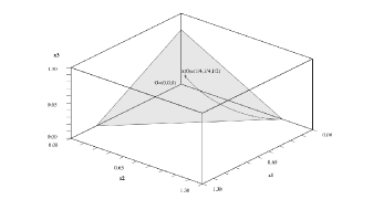
Figure 1: A trajectory of (35).

Karmarkar studied (35) in [29] for a quadratic objective function as a continuous model of the interior point algorithm introduced by him in [28]. Equation (34) is studied by Faybusovich in [18, 19, 20] when $(P)$ is a linear program, establishing connections with completely integrable Hamiltonian systems and exponential convergence rate, and by Herzel et al. in [23], who prove quadratic convergence for an explicit discretization.

Take now the log barrier kernel $\theta_{1}$ and $h(x)=-\sum_{i=1}^{n}\ln x_{i}.$ Since $\nabla^{2}h(x)=X^{-2}$ with $X$ defined as above, the associated differential equation is

$$\dot{x}+[I-X^{2}A^{T}(AX^{2}A^{T})^{-1}A]X^{2}\nabla f(x)=0.$$ (36)

This equation was considered by Bayer and Lagarias in [5] for a linear program. In the particular case $f(x)=\langle c,x\rangle$ and without linear equality constraints, (36) amounts to $\dot{x}+X^{2}c=0$, or $\dot{y}+c=0$ for $y=\nabla h(x)=-X^{-1}e$ with $e=(1,\cdots,1)\in\mathbb{R}^{n}$, which gives $x(t)=\left(1/(1/x_{1}^{0}+c_{1}t),...,1/(1/x_{n}^{0}+c_{n}t)\right)$, $T_{m}\leq t\leq T_{M},$ with $T_{m}=\max\{-1/x_{i}^{0}c_{i}\;|\;c_{i}>0\}$ and $T_{M}=\min\{-1/x_{i}^{0}c_{i}\;|\;c_{i}<0\}$ (see [5, pag. 515]). Denote by $\Pi_{A_{0}}$ the Euclidean orthogonal projection onto ${\cal A}_{0}$. To study the associated trajectories for a general linear program, it is introduced in [5] the Legendre transform coordinates $y=\Pi_{{\cal A}_{0}}\nabla h(x)=[I-A^{T}(AA^{T})^{-1}A]X^{-1}e$, which still linearizes (36) when $f$ is linear (see section 5 for an extension of this result), and permits to establish some remarkable analytic and geometric properties of the trajectories. A similar system was considered in [21, 34] as a continuous log-barrier method for nonlinear inequality constraints and with ${\cal A}_{0}=\mathbb{R}^{n}$.

New systems may be derived by choosing other kernels. For instance, taking $h(x)=-1/\gamma\sum_{i=1}^{n}x_{i}^{\gamma}$ with $\gamma\in(0,1)$, $A=(1,\ldots,1)\in\mathbb{R}^{1\times n}$ and $b=1$, we obtain

$$\dot{x}_{i}+\frac{x_{i}^{2-\gamma}}{1-\gamma}\left(\frac{\partial f}{\partial x_{i}}-\sum_{j=1}^{n}\frac{x_{j}^{2-\gamma}}{\sum_{k=1}^{n}x_{k}^{2-\gamma}}\frac{\partial f}{\partial x_{j}}\right)=0,\quad i=1,\ldots,n.$$ (37)

4.5 Convergence results for linear programming

Let us consider the specific case of a linear program

$$\min_{x\in\mathbb{R}^{n}}\{\langle c,x\rangle\mid Bx\geq d,\>Ax=b\},$$

where $A$ and $b$ are as in section 2.1, $c\in\mathbb{R}^{n}$, $B$ is a $p\times n$ full rank real matrix with $p\geq n$ and $d\in\mathbb{R}^{p}$. We assume that the optimal set satisfies

$$S(LP)\hbox{ is nonempty and bounded},$$ (38)

and there exists a Slater point $x^{0}\in\mathbb{R}^{n}$, $Bx^{0}>d$ and $Ax^{0}=b$. Take the Legendre function

$$h(x)=\sum_{i=1}^{n}\theta(g_{i}(x)),\quad g_{i}(x)=\langle B_{i},x\rangle-d_{i},$$ (39)

where $B_{i}\in\mathbb{R}^{n}$ is the $i$th-row of $B$ and the Legendre kernel $\theta$ satisfies $(H_{1})$. By (38), $(WP_{1})$ holds and therefore $(H\mbox{-}SD)$ is well-posed due to Theorem 4.1. Moreover, $x(t)$ is bounded and all its cluster points belong to $S(LP)$ by Proposition 4.1. The variational property (20) ensures the convergence of $x(t)$ and gives a variational characterization of the limit as well. Indeed, we have the following result:

Proposition 4.4.

Let $h$ be given by (39) with $\theta$ satisfying $(H_{1})$. Under (38), $(H\mbox{-}SD)$ is well-posed and $x(t)$ converges as $t\to+\infty$ to the unique solution $x^{*}$ of

$$\min_{x\in S(LP)}\sum\limits_{i\notin I_{0}}D_{\theta}(g_{i}(x),g_{i}(x^{0})),$$ (40)

where $I_{0}=\{i\in I\mid g_{i}(x)=0\mbox{ for all }x\in S(LP)\}$.

Proof.

Assume that $S(LP)$ is not a singleton, otherwise there is nothing to prove. The relative interior ${\rm ri}\>S(LP)$ is nonempty and moreover ${\rm ri}\>S(LP)=\{x\in\mathbb{R}^{n}\mid g_{i}(x)=0\mbox{ for }i\in I_{0},\>g_{i}(x)>0\mbox{ for }i\not\in I_{0},\>Ax=b\}$. By compactness of $S(LP)$ and strict convexity of $\theta\circ g_{i}$, there exists a unique solution $x^{*}$ of (40). Indeed, it is easy to see that $x^{*}\in{\rm ri}\>(LP)$. Let $\bar{x}\in S(LP)$ and $t_{j}\to+\infty$ be such that $x(t_{j})\to\bar{x}$. It suffices to prove that $\bar{x}=x^{*}$. When $\theta(0)<+\infty$, the latter follows by the same arguments as in Corollary 4.1. When $\theta(0)=+\infty$, the proof of [4, Theorem 3.1] can be adapted to our setting (see also [27, Theorem 2]). Set $x^{*}(t)=x(t)-\bar{x}+x^{*}$. Since $Ax^{*}(t)=b$ and $D_{h}(x,x^{0})=\sum_{i=1}^{m}D_{\theta}(g_{i}(x),g_{i}(x^{0}))$, (20) gives

$$\langle c,x(t)\rangle+\frac{1}{t}\sum_{i=1}^{m}D_{\theta}(g_{i}(x(t)),g_{i}(x^{0}))\leq\langle c,x^{*}(t)\rangle+\frac{1}{t}\sum_{i=1}^{m}D_{\theta}(g_{i}(x^{*}(t)),g_{i}(x^{0})).$$ (41)

But $\langle c,x(t)\rangle=\langle c,x^{*}(t)\rangle$ and $\forall i\in I_{0}$, $g_{i}(x^{*}(t))=g_{i}(x(t))>0$. Since $x^{*}\in{\rm ri}\>S(LP)$, for all $i\notin I_{0}$ and $j$ large enough, $g_{i}(x^{*}(t_{j}))>0$. Thus, the right-hand side of (41) is finite at $t_{j}$, and it follows that $\sum\limits_{i\notin I_{0}}D_{\theta}(g_{i}(\bar{x}),g_{i}(x^{0}))\leq\sum\limits_{i\notin I_{0}}D_{\theta}(g_{i}(x^{*}),g_{i}(x^{0})).$ Hence, $\bar{x}=x^{*}$. ∎

Rate of convergence. We turn now to the case where there is no equality constraint so that the linear program is

$$\min_{x\in\mathbb{R}^{n}}\{\langle c,x\rangle\mid Bx\geq d\}.$$ (42)

We assume that (42) admits a unique solution $a$ and we study the rate of convergence when $\theta$ is a Bregman function with zone $\mathbb{R}_{+}$. To apply Proposition 4.2, we need:

Lemma 4.4.

Set $C=\{x\in\mathbb{R}^{n}|Bx>d\}$. If (42) admits a unique solution $a\in\mathbb{R}^{n}$ then $\exists k_{0}>0$, $\forall y\in\overline{C}$, $\langle c,y-a\rangle\geq k_{0}{\cal N}(y-a)$, where ${\cal N}(x)=\sum_{i\in I}|\langle B_{i},x\rangle|$ is a norm on $\mathbb{R}^{n}$.

Proof.

Set $I_{0}=\{i\in I\mid\langle B_{i},a\rangle=d_{i}\}$. The optimality conditions for $a$ imply the existence of a multiplier vector $\lambda\in\mathbb{R}^{p}_{+}$ such that $\lambda_{i}[d_{i}-\langle B_{i},a\rangle]=0$, $\forall i\in I,$ and $c=\sum_{i\in I}\lambda_{i}B_{i}$. Let $y\in\overline{C}$. We deduce that $\langle c,y-a\rangle=N(y-a)$ where $N(x)=\sum_{i\in I_{0}}\lambda_{i}|\langle B_{i},x\rangle|$. By uniqueness of the optimal solution, it is easy to see that ${\rm span}\{B_{i}\mid i\in I_{0}\}=\mathbb{R}^{n}$, hence $N$ is a norm on $\mathbb{R}^{n}$. Since ${\cal N}(x)=\sum_{i\in I}|\langle B_{i},x\rangle|$ is also a norm on $\mathbb{R}^{n}$ (recall that $B$ is a full rank matrix), we deduce that $\exists k_{0}$ such that $N(x)\geq k_{0}{\cal N}(x)$. ∎

The following lemma is a sharper version of Proposition 4.2 in the linear context.

Lemma 4.5.

Under the assumptions of Proposition 4.4, assume in addition that $\theta$ is a Bregman function with zone $\mathbb{R}_{-}$ and that there exist $\alpha>0$, $\beta\geq 1$ and $\varepsilon>0$ such that

$$\forall s\in(0,\varepsilon),\>\alpha D_{\theta}(0,s)^{\beta}\leq s.$$ (43)

Then there exists positive constants $K,L,M$ such that for all $t>0$ the trajectory of $(H$-$SD)$ satisfies $D_{h}(a,x(t))\leq Ke^{-Lt}$ if $\beta=1$, and $D_{h}(a,x(t))\leq M/t^{\frac{1}{\beta-1}}$ if $\beta>1$.

Proof.

By Lemma 4.4, there exists $k_{0}$ such that for all $t>0$,

$$\langle c,x(t)-a\rangle\geq\sum_{i\in I}k_{0}|\langle B_{i},x(t)\rangle-\langle B_{i},a\rangle|.$$ (44)

Now, if we prove that $\exists\lambda>0$ such that

$$|\langle B_{i},x(t)\rangle-\langle B_{i},a\rangle|\geq\lambda D_{\theta}(\langle B_{i},a\rangle-d_{i},\langle B_{i},x(t)\rangle-d_{i})$$ (45)

for all $i\in I$ and for $t$ large enough, then from (44) it follows that $f(\cdot)=\langle c,\cdot\rangle$ satisfies the assumptions of Proposition 4.2 and the conclusion follows easily. Since $x(t)\rightarrow a$, to prove (45) it suffices to show that $\forall r_{0}\geq 0$, $\exists\eta,\mu>0$ such that $\forall s$, $|s-r_{0}|<\eta$, $\mu D_{\theta}(r_{0},s)^{\beta}\leq|r_{0}-s|.$ The case where $r_{0}=0$ is a direct consequence of (43). Let $r_{0}>0$. An easy computation yields $\frac{d^{2}}{ds^{2}}D_{\theta}(r_{0},s)_{|s=r_{0}}=\theta^{\prime\prime}(r_{0}),$ and by Taylor’s expansion formula

$$D_{\theta}(r_{0},s)=\frac{\theta^{\prime\prime}(r_{0})}{2}(s-r_{0})^{2}+o(s-r_{0})^{2}$$ (46)

with $\theta^{\prime\prime}(r_{0})>0$ due to $(H_{1})$(iii). Let $\eta$ be such that $\forall s$, $|s-r_{0}|<\eta$, $s>0$, $D_{\theta}(r_{0},s)\leq\theta^{\prime\prime}(r_{0})(s-r_{0})^{2}$ and $D_{\theta}(r_{0},s)\leq 1$; since $\beta\geq 1$, $D_{\theta}(r_{0},s)^{\beta}\leq D_{\theta}(r_{0},s)\leq\theta^{\prime\prime}(r_{0})|s-r_{0}|$. ∎

To obtain Euclidean estimates, the functions $s\mapsto D_{\theta}(r_{0},s)$, $r_{0}\in\mathbb{R}_{+}$ have to be locally compared to $s\mapsto|r_{0}-s|$. By (46) and the fact that $\theta^{\prime\prime}>0$, for each $r_{0}>0$ there exists $K,\eta>0$ such that $|r_{0}-s|\leq K\sqrt{D_{\theta}(r_{0},s)},\>\forall s,\>|r_{0}-s|<\eta.$ This shows that, in practice, the Euclidean estimate depends only on a property of the type (43). Examples:
$\bullet$ The Boltzmann-Shannon entropy $\theta_{3}(s)=s\ln(s)-s$ and $\theta_{6}(s)=s\ln s$ satisfy $D_{\theta_{i}}(0,s)=s$, $s>0$; hence for some $K,L>0$, $|x(t)-a|\leq Ke^{-Lt}$, $\forall t\geq 0$.
$\bullet$ With either $\theta_{4}(s)=-s^{\gamma}/\gamma$ or $\theta_{5}(s)=(\gamma s-s^{\gamma})/(1-\gamma)$, $\gamma\in(0,1)$, we have $D_{\theta_{i}}(0,s)=(1+1/\gamma)s^{\gamma}$, $s>0$; hence $|x(t)-a|\leq K/t^{\frac{\gamma}{2-2\gamma}}$, $\forall t>0.$

4.6 Dual convergence

In this section we focus on the case $C=\mathbb{R}^{n}_{++}$, so that the minimization problem is

$$\min\{f(x)\mid x\geq 0,\;Ax=b\}.$$

We assume

$$\hbox{$f$ is convex and }S(P)\neq\emptyset,$$ (47)

together with the Slater condition

$$\exists x^{0}\in\mathbb{R}^{n},\;x^{0}>0,\;Ax^{0}=b.$$ (48)

In convex optimization theory, it is usual to associate with $(P)$ the dual problem given by

$$\min\{p(\lambda)\mid\lambda\geq 0\},$$

where $p(\lambda)=\sup\{\langle\lambda,x\rangle-f(x)\mid Ax=b\}$. For many applications, dual solutions are as important as primal ones. In the particular case of a linear program where $f(x)=\langle c,x\rangle$ for some $c\in\mathbb{R}^{n}$, writing $\lambda=c+A^{T}y$ with $y\in\mathbb{R}^{m}$ the linear dual problem may equivalently be expressed as $\min\{\langle b,y\rangle\mid A^{T}y+c\geq 0\}$. Thus, $\lambda$ is interpreted as a vector of slack variables for the dual inequality constraints. In the general case, $S(D)$ is nonempty and bounded under (47) and (48), and moreover $S(D)=\{\lambda\in\mathbb{R}^{n}\mid\lambda\geq 0,\;\lambda\in\nabla f(x^{*})+{\rm Im}\>A^{T},\;\langle\lambda,x^{*}\rangle=0\}$, where $x^{*}$ is any solution of $(P)$; see for instance [24, Theorems VII.2.3.2 and VII.4.5.1].
Let us introduce a Legendre kernel $\theta$ satisfying $(H_{1})$ and define

$$h(x)=\sum_{i=1}^{n}\theta(x_{i}).$$ (49)

Suppose that $(H\mbox{-}SD)$ is well-posed. Integrating the differential inclusion (17), we obtain

$$\lambda(t)\in c(t)+{\rm Im}A^{T},$$ (50)

where $c(t)=\frac{1}{t}\int_{0}^{t}\nabla f(x(\tau))d\tau$ and $\lambda(t)$ is the dual trajectory defined by

$$\lambda(t)=\frac{1}{t}[\nabla h(x^{0})-\nabla h(x(t))].$$ (51)

Assume that $x(t)$ is bounded. From (47), it follows that $\nabla f$ is constant on $S(P)$, and then it is easy to see that $\nabla f(x(t))\to\nabla f(x^{*})$ as $t\to+\infty$ for any $x^{*}\in S(P)$. Consequently, $c(t)\to\nabla f(x^{*})$. By (51) together with [36, Theorem 26.5], we have $x(t)=\nabla h^{*}(\nabla h(x^{0})-t\lambda(t)),$ where the Fenchel conjugate $h^{*}$ is given by $h^{*}(\lambda)=\sum_{i=1}^{n}\theta^{*}(\lambda_{i}).$ Take any solution $\widetilde{x}$ of $A\widetilde{x}=b$. Since $Ax(t)=b$, we have $\widetilde{x}-\nabla h^{*}(\nabla h(x^{0})-t\lambda(t))\in{\rm Ker}\>A$. On account of (50), $\lambda(t)$ is the unique optimal solution of

$$\lambda(t)\in\mbox{\rm Argmin}\left\{\langle\widetilde{x},\lambda\rangle+\frac{1}{t}\sum_{i=1}^{n}\theta^{*}(\theta^{\prime}(x^{0}_{i})-t\lambda_{i})\mid\lambda\in c(t)+{\rm Im}A^{T}\right\}.$$ (52)

By $(H_{1})$(iii), $\theta^{\prime}$ is increasing in $\mathbb{R}_{++}$. Set $\eta=\lim_{s\to+\infty}\theta^{\prime}(s)\in(-\infty,+\infty]$. Since $\theta^{*}$ is a Legendre type function, ${\rm int}\>{\rm dom}\>\theta^{*}={\rm dom}\>\partial\theta^{*}={\rm Im}\>\partial\theta=(-\infty,\eta)$. From $(\theta^{*})^{\prime}=(\theta^{\prime})^{-1}$, it follows that $\lim_{u\to-\infty}(\theta^{*})^{\prime}(u)=0$ and $\lim_{u\to\eta^{-}}(\theta^{*})^{\prime}(u)=+\infty$. Consequently, (52) can be interpreted as a penalty approximation scheme of the dual problem $(D)$, where the dual positivity constraints are penalized by a separable strictly convex function. Similar schemes have been treated in [4, 14, 26]. Consider the additional condition

$$\hbox{Either }\theta(0)<\infty,\hbox{ or }S(P)\hbox{ is bounded, or $f$ is linear.}$$ (53)

As a direct consequence of [26, Propositions 10 and 11], we obtain that under (47), (48), (53) and $(H_{1})$, $\{\lambda(t)\mid t\to+\infty\}$ is bounded and its cluster points belong to $S(D)$. The convergence of $\lambda(t)$ is more difficult to establish. In fact, under some additional conditions on $\theta^{*}$ (see [14, Conditions $(H_{0})$-$(H_{1})$] or [26, Conditions (A7) and (A8)]) it is possible to show that $\lambda(t)$ converges to a particular element of the dual optimal set (the “$\theta^{*}$-center” in the sense of [14, Definition 5.1] or the $D_{h}(\cdot,x^{0})$-center as defined in [26, pag. 616]), which is characterized as the unique solution of a nested hierarchy of optimization problems on the dual optimal set. We will not develop this point here. Let us only mention that for all the examples of section 4.4, $\theta_{i}^{*}$ satisfies such additional conditions and consequently:

Proposition 4.5.

Under (47), (48) and (53), for each of the explicit Legendre kernels given in section 4.4, $\lambda(t)$ given by (51) converges to a particular dual solution.

5 Legendre transform coordinates

5.1 Legendre functions on affine subspaces

The first objective of this section is to slightly generalize the notion of Legendre type function to the case of functions whose domains are contained in an affine subspace of $\mathbb{R}^{n}$. We begin by noticing that the Legendre type property does not depend on canonical coordinates.

Lemma 5.1.

Let $g\in\Gamma_{0}(\mathbb{R}^{r})$, $r\geq 1$, and $T:\mathbb{R}^{r}\to\mathbb{R}^{r}$ an affine invertible mapping. Then $g$ is of Legendre type iff $g\circ T$ is of Legendre type.

Proof.

The proof is elementary and is left to the reader. ∎

From now on, ${\cal A}$ is the affine subspace defined by (1), whose dimension is $r=n-m$.

Definition 5.1.

A function $g\in\Gamma_{0}({\cal A})$ is said to be of Legendre type if there exists an affine invertible mapping $T:{\cal A}\to\mathbb{R}^{r}$ such that $g\circ T^{-1}$ is a Legendre type function in $\Gamma_{0}(\mathbb{R}^{r})$.

By Lemma 5.1, the previous definition is consistent.

Proposition 5.1.

Let $h\in\Gamma_{0}(\mathbb{R}^{n})$ be a function of Legendre type with $C={\rm int}\>{\rm dom}\>h$. If ${{\cal F}}=C\cap{\cal A}\neq\emptyset$ then the restriction $h_{|_{\cal A}}$ of $h$ to ${\cal A}$ is of Legendre type and moreover ${\rm int}_{\cal A}{\rm dom}\>h_{|_{\cal A}}={{\cal F}}$ (${\rm int}_{\cal A}B$ stands for the interior of $B$ in ${\cal A}$ as a topological subspace of $\mathbb{R}^{n}$).

Proof.

From the inclusions ${{\cal F}}\subset{\rm dom}\>h_{|_{\cal A}}\subset\overline{{{\cal F}}}=\overline{C}\cap{\cal A}$ and since ${\rm ri}\>\overline{{{\cal F}}}={{\cal F}}$, we conclude that ${\rm int}_{\cal A}{\rm dom}\>h_{|_{\cal A}}={{\cal F}}\neq\emptyset$. Let $T:\mathbb{R}^{r}\to{\cal A}$ be an invertible transformation with $Tz=Lz+x^{0}$ for all $z\in\mathbb{R}^{r}$, where $x^{0}\in{\cal A}$ and $L:\mathbb{R}^{r}\to{\cal A}_{0}$ is a nonsingular linear mapping. Define $k=h_{|_{\cal A}}\circ T$. Clearly, $k\in\Gamma_{0}(\mathbb{R}^{r})$. Let us prove that $k$ is essentially smooth. We have ${\rm dom}\>k=T^{-1}{\rm dom}\>h_{|_{\cal A}}$ and therefore ${\rm int}\>{\rm dom}\>k=T^{-1}{{\cal F}}$. Since $h$ is differentiable on $C$, we conclude that $k$ is differentiable on ${\rm int}\>{\rm dom}\>k$. Now, let $(z^{j})\in{\rm int}\>{\rm dom}\>k$ be a sequence that converges to a boundary point $z\in{\rm bd}\>{\rm dom}\>k$. Then, $Tz^{j}\in{\rm int}_{\cal A}{\rm dom}\>h_{|_{\cal A}}$ and $Tz^{j}\to Tz\in{\rm bd}_{\cal A}{\rm dom}\>h_{|_{\cal A}}\subset{\rm bd}\>{\rm dom}\>h$. Since $h$ is essentially smooth, $|\nabla h(Tz^{j})|\to+\infty$. Thus, to prove that $|\nabla k(z^{j})|\to+\infty$ it suffices to show that there exists $\lambda>0$ such that $|\nabla k(z^{j})|\geq\lambda|\nabla h(Tz^{j})|$ for all $j$ large enough. Note that $\nabla k(z^{j})=\nabla[h_{|_{\cal A}}\circ T](z^{j})=L^{*}\nabla h_{|_{\cal A}}(Tz^{j})=L^{*}\Pi_{{\cal A}_{0}}\nabla h(Tz^{j}),$ where $L^{*}:{\cal A}_{0}\to\mathbb{R}^{r}$ is defined by $\langle z,L^{*}x\rangle=\langle Lz,x\rangle$, $\forall(z,x)\in\mathbb{R}^{r}\times{\cal A}_{0}.$ Of course, $L^{*}$ is linear with ${\rm Ker}\>L^{*}=\{0\}$. Therefore $\frac{\nabla k(z^{j})}{|\nabla h(Tz^{j})|}=L^{*}\Pi_{{\cal A}_{0}}\frac{\nabla h(Tz^{j})}{|\nabla h(Tz^{j})|}.$ Let $\omega$ denote the nonempty and compact set of cluster points of the normalized sequence $\nabla h(Tz^{j})/|\nabla h(Tz^{j})|$, $j\in\mathbb{N}$. By Lemma 4.1, we have that $\omega\subset\{\nu\in N_{\overline{C}}(Tz)\>|\>|\nu|=1\},$ and consequently Lemma 4.2 yields $\Pi_{{\cal A}_{0}}\omega\cap\{0\}=\emptyset.$ By compactness of $\omega$, we obtain $\liminf_{j\to+\infty}|\Pi_{{\cal A}_{0}}\nabla h(Tz^{j})|/|\nabla h(Tz^{j})|>0,$ which proves our claim. Finally, the strict convexity of $k$ on ${\rm dom}\>\partial k={\rm int}\>{\rm dom}\>k=T^{-1}{{\cal F}}$ is a direct consequence of the strict convexity of $h$ in ${{\cal F}}$. ∎

5.2 Legendre transform coordinates

The prominent fact of Legendre functions theory is that $h\in\Gamma_{0}(\mathbb{R}^{n})$ is of Legendre type iff its Fenchel conjugate $h^{*}$ is of Legendre type [36, Theorem26.5], and $\nabla h:{\rm int}\>{\rm dom}\>h\to{\rm int}\>{\rm dom}\>h^{*}$ is onto with $(\nabla h)^{-1}=\nabla h^{*}$. In the case of Legendre functions on affine subspaces, we have the following generalization:

Proposition 5.2.

If $g\in\Gamma_{0}({\cal A})$ is of Legendre type in the sense of Definition 5.1, then $\nabla g({\rm int}_{\cal A}{\rm dom}\>g)$ is a nonempty, open and convex subset of ${\cal A}_{0}$. In addition, $\nabla g$ is a one-to-one continuous mapping from ${\rm int}_{\cal A}{\rm dom}\>g$ onto its image.

Proof.

Let $Tx=Lx+z_{0}$ with $L:{\cal A}_{0}\to\mathbb{R}^{r}$ being a linear invertible mapping and $z_{0}\in\mathbb{R}^{p}$. Set $k=g\circ T^{-1}\in\Gamma_{0}(\mathbb{R}^{r})$, which is of Legendre type. We have ${\rm dom}\>k=T{\rm dom}\>g$. Define $L^{*}:\mathbb{R}^{r}\to{\cal A}_{0}$ by $\langle L^{*}z,x\rangle=\langle z,Lx\rangle$, $\forall(z,x)\in\mathbb{R}^{r}\times{\cal A}_{0}$. We have that $\nabla g(x)=\nabla[k\circ T](x)=L^{*}\nabla k(Tx)$ for all $x\in{\rm int}_{\cal A}{\rm dom}\>g$. Therefore $\nabla g({\rm int}_{\cal A}{\rm dom}\>g)=L^{*}\nabla k(T{\rm int}_{\cal A}{\rm dom}\>g)=L^{*}\nabla k({\rm int}_{\mathbb{R}^{r}}{\rm dom}\>k)=L^{*}{\rm int}_{\mathbb{R}^{r}}{\rm dom}\>k^{*}.$ Since ${\rm int}_{\mathbb{R}^{r}}{\rm dom}\>k^{*}$ is a nonempty, open and convex subset of $\mathbb{R}^{r}$ and $L^{*}$ is an invertible linear mapping, then $L^{*}{\rm int}_{\mathbb{R}^{r}}{\rm dom}\>k^{*}$ is an open and nonempty subset of ${\cal A}_{0}$. Moreover, by [36, Theorem 6.6], we have $L^{*}{\rm int}_{\mathbb{R}^{r}}{\rm dom}\>k^{*}={\rm ri}\>L^{*}{\rm dom}\>k^{*}.$ Consequently, $\nabla g({\rm int}_{\cal A}{\rm dom}\>g)={\rm ri}\>L^{*}{\rm dom}\>k^{*}={\rm int}_{{\cal A}_{0}}L^{*}{\rm dom}\>k^{*}\neq\emptyset.$ Finally, since $\nabla k:{\rm int}_{\mathbb{R}^{r}}{\rm dom}\>k\to{\rm int}_{\mathbb{R}^{r}}{\rm dom}\>k^{*}$ is one-to-one and continuous, the same result holds for $\nabla g=L^{*}\circ\nabla k\circ T$ on ${\rm int}_{\cal A}{\rm dom}\>g$. ∎

In the sequel, we assume that $h$ satisfies the basic condition $(H_{0})$ and ${{\cal F}}=C\cap{\cal A}\neq\emptyset$. The Legendre transform coordinates mapping on ${{\cal F}}$ associated with $h$ is defined by

$$\begin{array}[]{cccl}\phi_{h}:&{{\cal F}}&\to&{{\cal F}}^{*}=\phi_{h}({{\cal F}})\\ &x&\mapsto&\phi_{h}(x)=\nabla(h_{|_{\cal A}})=\Pi_{{\cal A}_{0}}\nabla h(x).\end{array}$$ (54)

This definition retrieves the Legendre transform coordinates introduced by Bayer and Lagarias in [5] for the particular case of the log-barrier on a polyhedral set.

Theorem 5.1.

Under the above definitions and assumptions, ${{\cal F}}^{*}$ is a convex, (relatively) open and nonempty subset of ${\cal A}_{0}$, $\phi_{h}$ is a ${\cal C}^{1}$ diffeomorphism from ${{\cal F}}$ to ${{\cal F}}^{*}$, and for all $x\in{{\cal F}}$, $d\phi_{h}(x)=\Pi_{{\cal A}_{0}}H(x)$ and $d\phi_{h}(x)^{-1}=\sqrt{H(x)^{-1}}\Pi_{\sqrt{H(x)}{\cal A}_{0}}\sqrt{H(x)^{-1}}$, where $H(x)=\nabla^{2}h(x)$.

Proof.

By Propositions 5.1 and 5.2, ${{\cal F}}^{*}$ is a convex, open and nonempty subset of ${\cal A}_{0}$ and $\phi_{h}$ is a continuous bijection. By $(H_{0})$(ii), $\phi_{h}$ is of class ${\cal C}^{1}$ on ${{\cal F}}$ and we have for all $x\in{{\cal F}}$, $d\phi_{h}(x)=\Pi_{{\cal A}_{0}}\nabla^{2}h(x)=\Pi_{{\cal A}_{0}}H(x).$ Let $v\in{\cal A}_{0}$ be such that $d\phi_{h}(x)v=0$. It follows that $H(x)v\in{\cal A}_{0}^{\perp}$ and in particular $\langle H(x)v,v\rangle=0$. Hence, $v=0$ thanks to $(H_{0})$(iii). The implicit function theorem implies then that $\phi_{h}$ is a ${\cal C}^{1}$ diffeomorphism. The formula concerning $d\phi_{h}(x)^{-1}$ is a direct consequence of the next lemma.

Lemma 5.2.

Define the linear operators $L_{i}:\mathbb{R}^{n}\to\mathbb{R}^{n}$ by $L_{1}=\Pi_{{\cal A}_{0}}H(x)$ and $L_{2}=\sqrt{H(x)^{-1}}\Pi_{\sqrt{H(x)}{\cal A}_{0}}\sqrt{H(x)^{-1}}$. Then $L_{2}L_{1}v=v$ for all $v\in{\cal A}_{0}$.

This follows by the same method as in [5], pag. 545; we leave the proof to the reader. ∎

Similarly to the classical Legendre type functions theory, the inverse of $\phi_{h}$ can be expressed in terms of Fenchel conjugates. For that purpose, we notice that inverting $\phi_{h}$ is a minimization problem. Indeed, given $y\in{\cal A}_{0}$, the problem of finding $x\in{{\cal F}}$ such that $y=\Pi_{{\cal A}_{0}}\nabla h(x)$ is equivalent to $x=\mbox{\rm Argmin}\{h(z)-\langle y,z\rangle|z\in{\cal A}\}$, or equivalently

$$x=\mbox{\rm Argmin}\{(h+\delta_{{\cal A}})(z)-\langle y,z\rangle\},$$ (55)

where $\delta_{{\cal A}}$ is the indicator of ${\cal A}$, i.e. $\delta_{{\cal A}}(z)=0$ if $z\in{\cal A}$ and $+\infty$ otherwise. Let us recall the definition of epigraphical sum of two functions $g_{1},g_{2}\in\Gamma_{0}(\mathbb{R}^{n})$, which is given by $\left(g_{1}\square g_{2}\right)(y)=\inf\{g_{1}(u)+g_{2}(v)|u+v=y\}$, $\forall y\in\mathbb{R}^{n}.$ We have $g_{1}\square g_{2}\in\Gamma_{0}(\mathbb{R}^{n})$ and if $g_{1}$ and $g_{2}$ satisfy ${\rm ri}\>{\rm dom}\>g_{1}\cap{\rm ri}\>{\rm dom}\>g_{2}\neq\emptyset$ then $(g_{1}+g_{2})^{*}=g_{1}^{*}\square g_{2}^{*}$ (see [36]).

Proposition 5.3.

We have that $\phi_{h}^{-1}:{{\cal F}}^{*}\to{{\cal F}}$ is given by $\phi_{h}^{-1}(y)=\nabla[h^{*}\square(\delta_{{\cal A}_{0}^{\perp}}+\langle\cdot,\widetilde{x}\rangle)](y),$ for any $\widetilde{x}\in{\cal A}$, and moreover ${{\cal F}}^{*}=\Pi_{{\cal A}_{0}}{\rm int}\>{\rm dom}\>h^{*}$.

Proof.

The optimality condition for (55) yields $y\in\partial(h+\delta_{{\cal A}})(x).$ Thus, $x\in\partial(h+\delta_{\cal A})^{*}(y)$. From ${{\cal F}}\neq\emptyset$, we conclude that the function $g\in\Gamma_{0}(\mathbb{R}^{n})$ defined by $g=(h+\delta_{\cal A})^{*}$ satisfies $g=h^{*}\square\delta_{\cal A}^{*}=h^{*}\square(\delta_{{\cal A}_{0}^{\perp}}+\langle\cdot,\widetilde{x}\rangle)$ with $\widetilde{x}\in{\cal A}$. Moreover, by [36, Corollary 26.3.2], $g$ is essentially smooth and we deduce that indeed $x=\nabla g(y)$. Since $g$ is essentially smooth, ${\rm dom}\>\partial g={\rm int}\>{\rm dom}\>g$. By definition of epigraphical sum, $g(y)=\inf\{h^{*}(u)+\delta_{{\cal A}_{0}^{\perp}}(v)+\langle v,\widetilde{x}\rangle|u+v=y\},$ and consequently we have that $y\in{\rm dom}\>g$ iff $y\in{\rm dom}\>h^{*}+{\cal A}_{0}^{\perp}$. Hence, ${\rm int}\>{\rm dom}\>g={\rm int}\>{\rm dom}\>h^{*}+{\cal A}_{0}^{\perp}$ (see for instance [36, Corollary 6.6.2]). Recalling that ${{\cal F}}^{*}$ is a relatively open subset of ${\cal A}_{0}$, we deduce that ${{\cal F}}^{*}=\Pi_{{\cal A}_{0}}{\rm dom}\>\partial g=\Pi_{{\cal A}_{0}}{\rm int}\>{\rm dom}\>h^{*}$. ∎

5.3 Linear problems in Legendre transform coordinates

5.3.1 Polyhedral sets in Legendre transform coordinates

One of the first interest of Legendre transform coordinates is to transform linear constraints into positive cones.

Proposition 5.4.

Assume that $C=\{x\in\mathbb{R}^{n}|Bx>d\}$, where $B$ is a $p\times n$ full rank matrix, with $p\geq n$. Suppose also that $h$ is of the form (39) with $\theta$ satisfying $(H_{1})$, and let $\eta=\lim_{s\to+\infty}\theta^{\prime}(s)\in(-\infty,+\infty]$. If $\eta<+\infty$ then $\overline{{\rm dom}\>h^{*}}=\{y\in\mathbb{R}^{n}\mid y+B^{T}\lambda=0,\;\lambda_{i}\geq-\eta\},$ and ${\rm dom}\>h^{*}=\mathbb{R}^{n}$ when $\eta=+\infty$.

Proof.

By [37, Theorem 11.5], $\overline{{\rm dom}\>h^{*}}=\{y\in\mathbb{R}^{n}\mid\langle y,d\rangle\leq h^{\infty}(d)\hbox{ for all }d\in\mathbb{R}^{n}\}$, where $h^{\infty}$ is the recession function, also known as horizon function, of $h$. The recession function is defined by $h^{\infty}(d)=\lim_{t\to+\infty}\frac{1}{t}[h(\bar{x}+td)-h(\bar{x})],\;d\in\mathbb{R}^{n}$, where $\bar{x}\in{\rm dom}\>h$; this limit does not depend of $\bar{x}$ and eventually $h^{\infty}(d)=+\infty$ (see also [36]). In this case, it is easy to verify that $h^{\infty}(d)=\sum_{i=1}^{p}\theta^{\infty}(\langle B_{i},d\rangle).$ Clearly, $\theta^{\infty}(-1)=+\infty$ and $\theta^{\infty}(1)=\lim_{s\to+\infty}\theta^{\prime}(s)=\eta$. In particular, if $\eta=+\infty$ then ${\rm dom}\>h^{*}=\mathbb{R}^{n}$. If $\eta<+\infty$ then $y\in\overline{{\rm dom}\>h^{*}}$ iff for all $d\in\mathbb{R}^{n}$ such that $Bd\geq 0$, $\langle y,d\rangle\leq h^{\infty}(d)=\sum_{i=1}^{p}\eta\langle B_{i},d\rangle$, that is $\langle y-\eta B^{T}e,d\rangle\leq 0$ with $e=(1,\cdots,1)$. Thus, by the Farkas lemma, $y\in\overline{{\rm dom}\>h^{*}}$ iff $\exists\mu\geq 0$, $y-\eta B^{T}e+B^{T}\mu=0$. ∎

As a direct consequence of Propositions 5.3 and 5.4:

Corollary 5.1.

Under the assumptions of Proposition 5.4, if $\eta=0$ then ${{\cal F}}^{*}$ is a positive convex cone and if $\eta=+\infty$ then ${{\cal F}}^{*}={\cal A}_{0}$.

5.3.2 $(H\mbox{-}SD)$-trajectories in Legendre transform coordinates

In the sequel, we assume that $f(x)=\langle c,x\rangle$ for some $c\in\mathbb{R}^{n}$. As another striking application of Legendre transform coordinates, we prove now that the trajectories of $(H\mbox{-}SD)$ may be seen as straight lines in ${{\cal F}}^{*}$. Recall that the push forward vector field of $\nabla_{{}_{H}}f_{|_{{\cal F}}}$ by $\phi_{h}$ is defined for every $y\in{{\cal F}}^{*}$ by $[(\phi_{h})_{*}\nabla_{{}_{H}}f_{|_{{{\cal F}}}}]\>(y)=d\phi_{h}(\phi_{h}^{-1}(y))\nabla_{{}_{H}}f_{|_{{\cal F}}}(\phi_{h}^{-1}(y))$.

Proposition 5.5.

For all $y\in{{\cal F}}^{*}$, $[(\phi_{h})_{*}\nabla_{{}_{H}}f_{|_{{\cal F}}}]\>(y)=\Pi_{{\cal A}_{0}}c.$

Proof.

Let $y\in{{\cal F}}^{*}$. Setting $x=\phi_{h}^{-1}(y)$, by Theorem 5.1 we get $[(\phi_{h})_{*}\nabla_{{}_{H}}f_{|_{{{\cal F}}}}]\>(y)=d\phi_{h}(x)\nabla_{{}_{H}}f_{|_{{\cal F}}}(x)=\Pi_{{\cal A}_{0}}H(x)H(x)^{-1}[I-A^{T}(AH(x)^{-1}A^{T})^{-1}AH(x)^{-1}]c=\Pi_{{\cal A}_{0}}c-\Pi_{{\cal A}_{0}}A^{T}z,$ where $z=[(AH(x)^{-1}A^{T})^{-1}AH(x)^{-1}]c.$ Since ${\rm Im}\>A^{T}={\cal A}_{0}^{\perp}$, the conclusion follows. ∎

Next, we give two optimality characterizations of the orbits of $(H\mbox{-}SD)$, extending thus to the general case the results of [5] for the log-metric.

5.3.3 Geodesic curves

First, we claim that the orbits of $(H\mbox{-}SD)$ can be regarded as geodesics curves with respect to some appropriate metric on ${{\cal F}}$. To this end, we endow ${{\cal F}}^{*}=\phi_{h}({{\cal F}})$ with the Euclidean metric, which allows us to define on ${{\cal F}}$ the metric

$$(\cdot,\cdot)^{H^{2}}=\left(\phi_{h}\right)^{*}\langle\cdot,\cdot\rangle,$$ (56)

that is, $\forall(x,u,v)\in{{\cal F}}\times\mathbb{R}^{n}\times\mathbb{R}^{n}$, $(u,v)^{H^{2}}_{x}=\langle d\phi_{h}(x)u,d\phi_{h}(x)v\rangle=\langle\Pi_{{\cal A}_{0}}H(x)u,\Pi_{{\cal A}_{0}}H(x)v\rangle.$ For each initial condition $x^{0}\in{{\cal F}}$, and for every $c\in\mathbb{R}^{n}$ we set

$$v=d\phi_{h}(x^{0})^{-1}\Pi_{{\cal A}_{0}}c=\sqrt{H(x^{0})^{-1}}\Pi_{\sqrt{H(x^{0})}{\cal A}_{0}}\sqrt{H(x^{0})^{-1}}\Pi_{{\cal A}_{0}}c.$$ (57)

Theorem 5.2.

Let $(x^{0},c)\in{{\cal F}}\times\mathbb{R}^{n}$, set $f(x)=\langle c,x\rangle,\>\forall x\in C$ and define $v$ as in (57). If ${{\cal F}}$ is endowed with the metric $(\cdot,\cdot)^{H^{2}}$ given by (56), then the solution $x(t)$ of $(H\mbox{-}SD)$ is the unique geodesic passing through $x^{0}$ with velocity $v$.

Proof.

Since ${{\cal F}},\>(\cdot,\cdot)^{H^{2}}$ is isometric to the Euclidean Riemannian manifold ${{\cal F}}^{*}$, the geodesic joining two points of ${{\cal F}}$ exists and is unique. Let us denote by $\gamma:J\subset\mathbb{R}\mapsto{{\cal F}}$ the geodesic passing through $x^{0}$ with velocity $v$. By definition of $(\cdot,\cdot)^{H^{2}}$, $\phi_{h}(\gamma)$ is a geodesic in ${{\cal F}}^{*}$. Whence $\phi_{h}(\gamma(t))=\phi_{h}(x^{0})+td\phi_{h}(x^{0})v,$ where $t\in J$. In view of (57), this can be rewritten $\phi_{h}(\gamma(t))=\phi_{h}(x^{0})+t\Pi_{{\cal A}_{0}}c$. By Proposition 5.5 we know that $\left(\phi_{h}\right)_{*}\nabla_{{}_{H}}f_{|{{\cal F}}}=\Pi_{{\cal A}_{0}}c$, and therefore $\phi_{h}^{-1}(\phi_{h}(\gamma))=\gamma$ is exactly the solution of $(H\mbox{-}SD)$.∎

Remark 5.1.

A Riemannian manifold is called geodesically complete if the maximal interval of definition of every geodesic is $\mathbb{R}$. When $\Pi_{{\cal A}_{0}}c\neq 0$ and ${{\cal F}}^{*}$ is not an affine subspace of $\mathbb{R}^{n}$, the Riemannian manifold ${{\cal F}},\>(\cdot,\cdot)^{H^{2}}$ is not complete in this sense.

5.3.4 Lagrange equations

Following the ideas of [5], we describe the orbits of $(H\mbox{-}SD)$ as orthogonal projections on ${\cal A}$ of $\dot{q}-$trajectories of a specific Lagrangian system. Recall that given a real-valued mapping ${\cal L}(q,\dot{q})$ called the Lagrangian, where $q=(q_{1},\dots,q_{n})$ and $\dot{q}=(\dot{q}_{1},\dots,\dot{q}_{n})$, the associated Lagrange equations of motion are the following

$$\frac{d}{dt}\frac{\partial{\cal L}}{\partial\dot{q}_{i}}=\frac{\partial{\cal L}}{\partial q_{i}},\quad\frac{d}{dt}q_{i}=\dot{q}_{i},\quad\forall i=1\dots n.$$ (58)

Their solutions are $C^{1}-$piecewise paths $\gamma:t\longmapsto(q(t),\dot{q}(t))$, defined for $t\in J\subset\mathbb{R}$, that satisfy (58), and appear as extremals of the functional $\widehat{{\cal L}}(\gamma)=\int_{J}{\cal L}(q(t),\dot{q}(t))dt$. Notice that in general, the solutions are not unique, in the sense that they do not only depend on the initial condition $\gamma(0)$. Let us introduce the Lagrangian ${\cal L}:\mathbb{R}^{n}\times C\to\mathbb{R}$ defined by

$${\cal L}(q,\dot{q})=\langle\Pi_{{\cal A}_{0}}c,q\rangle-h(\Pi_{{\cal A}}\dot{q}),$$ (59)

where $\Pi_{{\cal A}}$ is the orthogonal projection onto ${\cal A}$, i.e. $\Pi_{{\cal A}}x=\widetilde{x}+\Pi_{{\cal A}_{0}}(x-\widetilde{x})$ for any $\widetilde{x}\in{\cal A}$.

Theorem 5.3.

For any solution $\gamma(t)=(q(t),\dot{q}(t))$ of the Lagrangian dynamical system (58) with Lagrangian given by (59), the projection $x(t)=\Pi_{{\cal A}}\dot{q}(t)$ is the solution of (H-SD) with initial condition $x^{0}=\Pi_{{\cal A}}\dot{q}(0).$

Proof.

It is easy to verify that $\nabla(h\circ\Pi_{{\cal A}})(x)=\Pi_{{\cal A}_{0}}\nabla h(\Pi_{{\cal A}}x)$ for any $x\in\mathbb{R}^{n}.$ Given a solution $\gamma(t)=(q(t),\dot{q}(t))$ of (59) defined on $J$, we set $p(t)=(p_{1}(t),\dots,p_{n}(t))=\left(\frac{\partial{\cal L}}{\partial\dot{q}_{1}}(\gamma(t)),\dots,\frac{\partial{\cal L}}{\partial\dot{q}_{n}}(\gamma(t))\right)$. We have $p(t)=\nabla(h\circ\Pi_{{\cal A}})(\dot{q}(t))=\Pi_{{\cal A}_{0}}\nabla h(\Pi_{{\cal A}}\dot{q}(t))=\phi_{h}(\Pi_{{\cal A}}\dot{q}(t)).$ Equations of motion become $\frac{d}{dt}p(t)=\Pi_{{\cal A}_{0}}c,$ that is, $\frac{d}{dt}\phi_{h}(\Pi_{{\cal A}}\dot{q}(t))=\Pi_{{\cal A}_{0}}c$. Since $\phi_{h}:{{\cal F}}\to{{\cal F}}^{*}$ is a diffeomorphism, the latter means, according to Proposition 5.5, that $\Pi_{{\cal A}}\dot{q}(t)$ is a trajectory for the vector field $\nabla_{H}f_{|_{{\cal F}}}.$ Notice that $C$ being convex, as soon as $\dot{q}(0)\in C,$ $\Pi_{{\cal A}}\dot{q}(0)\in C\cap{\cal A}={{\cal F}},$ and what precedes forces $\Pi_{{\cal A}}\dot{q}(t)$ to stay in ${{\cal F}}$ for any $t\in J.$ ∎

5.3.5 Completely integrable Hamiltonian systems

In the sequel, all mappings are supposed to be at least of class ${\cal C}^{2}$. Let us first recall the notion of Hamiltonian system. Given an integer $r\geq 1$ and a real-valued mapping ${\cal H}(q,p)$ on $\mathbb{R}^{2r}$ with coordinates $(q,p)=(q_{1},\dots,q_{r},p_{1},\dots,p_{r})$, the Hamiltonian vector field $X_{{\cal H}}$ associated with ${\cal H}$ is defined by $X_{{\cal H}}=\sum_{i=1}^{r}\frac{\partial{\cal H}}{\partial p_{i}}\frac{\partial}{\partial q_{i}}-\frac{\partial{\cal H}}{\partial q_{i}}\frac{\partial}{\partial p_{i}}.$ The trajectories of the dynamical system induced by $X_{{\cal H}}$ are the solutions to

$$\left\{\begin{array}[]{l}\dot{p}_{i}(t)=-\frac{\partial}{\partial q_{i}}{\cal H}(q(t),p(t)),\>i=1,\dots,r,\\ \dot{q}_{i}(t)=\frac{\partial}{\partial p_{i}}{\cal H}(q(t),p(t)),\>i=1,\dots,r.\end{array}\right.$$ (60)

Following a standard procedure, Lagrangian functions ${\cal L}(q,\dot{q})$ are associated with Hamiltonian systems by means of the so-called Legendre transform

$$\Phi:\left\{\begin{array}[]{ccl}\mathbb{R}^{2r}&\longrightarrow&\mathbb{R}^{2r}\\ (q,\dot{q})&\longmapsto&(q,\frac{\partial{\cal L}}{\partial\dot{q}}(q,\dot{q}))\end{array}\right.$$

In fact, when $\Phi$ is a diffeomorphism, the Hamiltonian function ${\cal H}$ associated with the Lagrangian ${\cal L}$ is defined on $\Phi(\mathbb{R}^{2r})$ by ${\cal H}(p,q)=\sum_{i=1}^{r}p_{i}\dot{q}_{i}-{\cal L}(q,\dot{q})=\langle p,\psi^{-1}(q,p)\rangle-{\cal L}(q,\psi^{-1}(q,p)),$ where $(q,\psi^{-1}(q,p)):=\Phi^{-1}(q,p)$. With these definitions, $\Phi$ sends the trajectories of the corresponding Lagrangian system on the trajectories of the Hamiltonian system (60).

In general, the Lagrangian (59) does not lead to an invertible $\Phi$ on $\mathbb{R}^{2n}$. However, we are only interested in the projections $\Pi_{{\cal A}}\dot{q}$ of the trajectories, which, according to Theorem 5.3, take their values in ${{\cal F}}$. Moreover, notice that for any differentiable path $t\mapsto q^{\perp}(t)$ lying in ${\cal A}_{0}^{\perp}$, $t\mapsto(q(t),\dot{q}(t))$ is a solution of (58) iff $t\mapsto(q(t)+q^{\perp}(t),\dot{q}(t)+\dot{q}^{\perp}(t))$ is. This legitimates the idea of restricting ${\cal L}$ to ${\cal A}_{0}\times\Pi_{{\cal A}_{0}}{{\cal F}}$. Hence and from now on, ${\cal L}$ denotes the function:

$${\cal L}:\left\{\begin{array}[]{ccl}{\cal A}_{0}\times\Pi_{{\cal A}_{0}}{{\cal F}}&\longrightarrow&\mathbb{R}\\ (q,\dot{q})&\longmapsto&{\cal L}(q,\dot{q}).\end{array}\right.$$ (61)

Taking $(q_{1},\dots,q_{r})$, with $r=n-m$, a linear system of coordinates induced by an Euclidean orthonormal basis for ${\cal A}_{0}$, we easily see that this “new” Lagrangian has trajectories $(q(t),\dot{q}(t))$ lying in ${\cal A}_{0}\times\Pi_{{\cal A}_{0}}{{\cal F}}$, whose projections $\Pi_{{\cal A}}\dot{q}(t)$ are exactly the $(H\mbox{-}SD)$ trajectories. Moreover, an easy computation yields

$$\frac{\partial{\cal L}}{\partial\dot{q}}(q,\dot{q})=\Pi_{{\cal A}_{0}}\nabla h(\Pi_{{\cal A}_{0}}\dot{q})=[\phi_{h}\circ\Pi_{{\cal A}}](\dot{q}),$$

which is a diffeomorphism by Proposition 5.1. The Legendre transform is then given by

$$\Phi:\left\{\begin{array}[]{ccl}{\cal A}_{0}\times\Pi_{{\cal A}_{0}}{{\cal F}}&\longrightarrow&{\cal A}_{0}\times{{\cal F}}^{*}\\ (q,\dot{q})&\longmapsto&(q,[\phi_{h}\circ\Pi_{{\cal A}}](\dot{q})),\end{array}\right.$$

and therefore, ${\cal L}$ is converted into the Hamiltonian system associated with

$${\cal H}:\left\{\begin{array}[]{ccl}{\cal A}_{0}\times{{\cal F}}^{*}&\longrightarrow&\mathbb{R}\\ (q,p)&\longmapsto&\langle p,[\phi_{h}\circ\Pi_{{\cal A}}]^{-1}(p)\rangle-{\cal L}(q,[\phi_{h}\circ\Pi_{{\cal A}}]^{-1}(p)).\end{array}\right.$$ (62)

Let us now introduce the concept of completely integrable Hamiltonian system. The Poisson bracket of two real valued functions $f_{1},f_{2}$ on $\mathbb{R}^{2r}$ is given by $\{f_{1},f_{2}\}=\sum_{i=1}^{r}\frac{\partial f_{1}}{\partial p_{i}}\frac{\partial f_{2}}{\partial q_{i}}-\frac{\partial f_{1}}{\partial q_{i}}\frac{\partial f_{2}}{\partial p_{i}}.$ Notice that, from the definitions, we have $\{f_{1},f_{2}\}=X_{f_{1}}(f_{2})$ and $X_{\{f_{1},f_{2}\}}=[X_{f_{1}},X_{f_{2}}]$, where $[\cdot,\cdot]$ is the standard bracket product of vector fields [33]. Now, the system (60) is called completely integrable if there exist $r$ functions $f_{1},\dots,f_{r}$ with $f_{1}={\cal H}$, satisfying

$$\left\{\begin{array}[]{l}\{f_{i},f_{j}\}=0,\quad\forall i,j=1,\dots,r.\\ df_{1}(x),\dots,df_{r}(x)\textrm{ are linearly independent at any }x\in\mathbb{R}^{2r}.\end{array}\right.$$

As a motivation for completely integrable systems, we will just point out the following: the functions $f_{i}$ are called integrals of motions because $X_{{\cal H}}(f_{i})=\{h,f_{i}\}=0$, which means that any trajectory of $X_{{\cal H}}$ lies on the level sets of each $f_{i}$ (the same holds for all $X_{f_{j}}$). Also, the trajectory passing through $(q_{0},p_{0})$ lies in the set $\bigcap_{i=1\dots r}f^{-1}_{i}(\{f_{i}(q_{o},p_{0})\})$. Besides, $[X_{f_{i}},X_{f_{j}}]=0$ implies that we can find, at least locally, coordinates $(x_{1},\dots,x_{r})$ on this set such that $X_{{\cal H}}=\frac{\partial}{\partial x_{1}},X_{f_{2}}=\frac{\partial}{\partial x_{2}},\dots,X_{f_{r}}=\frac{\partial}{\partial x_{r}},$ that is, in these coordinates, the trajectories of $X_{f_{i}}$ are straight lines.

Theorem 5.4.

Suppose $\Pi_{A_{0}}c\neq 0.$ The Lagrangian system on ${\cal A}_{0}\times\Pi_{{\cal A}_{0}}{{\cal F}}$ associated with (59), (61) gives rise, by the Legendre transform, to a completely integrable Hamiltonian system on ${\cal A}_{0}\times{{\cal F}}^{*}$ with Hamiltonian given by (62).

Proof.

There only remains to prove the complete integrability of the system. To this end, we adapt the proof of [5, Theorem II.12.2] to our abstract framework. Take the integrals of motion to be $f_{1}={\cal H}$, $f_{i}(q,p)=\langle c_{i},p\rangle,\>i=2,\dots,r$ where $r=n-m$ and $\{\Pi_{{\cal A}_{0}}c,\>c_{2},\dots,c_{r}\}$ is chosen as to be an orthonormal basis of ${\cal A}_{0}$. For any $i,j\in\{2,\dots,r\},$ $\{f_{i},f_{j}\}$ is zero since $f_{i}$ and $f_{j}$ only depend on $p$. Let $\phi_{h,l}^{-1}(q,p)$ (resp. $(\Pi_{{\cal A}_{0}}c)_{l}$) stand for the $l$-th component of $\phi_{h}^{-1}(q,p)$ (resp. the $l$-th component of $\Pi_{{\cal A}_{0}}c$) and take some $k\in\{1,...,r\}$. Since

$$\frac{\partial{\cal H}}{\partial q_{k}}(q,p) = \frac{\partial(\sum_{l=1}^{r}p_{l}\phi^{-1}_{h,l})}{\partial q_{k}}(q,p)-\frac{\partial({\cal L}\circ\Phi^{-1})}{\partial q_{k}}(q,p)$$

$$= \sum_{l=1}^{r}p_{l}\frac{\partial\phi_{h,l}^{-1}}{\partial q_{k}}(p,q)-\frac{\partial{\cal L}}{\partial q_{k}}(q,\phi_{h}^{-1}(q,p))-\sum_{l=1}^{r}\frac{\partial{\cal L}}{\partial\dot{q}_{l}}(q,\phi_{h}^{-1}(q,p))\frac{\partial\phi_{h,l}}{\partial q_{k}}(q,p)$$

$$= -(\Pi_{{\cal A}_{0}}c)_{k}$$

we deduce that for all $i\in\{2,...,r\}$, $\{{\cal H},f_{i}\}=\sum_{k=1}^{r}-\frac{\partial f_{i}}{\partial p_{k}}\frac{\partial{\cal H}}{\partial q_{k}}=\langle\Pi_{{\cal A}_{0}}c,c_{i}\rangle=0$. The second condition for complete integrability is satisfied too, as the $r\times 2r$ matrix

$$\left([\frac{\partial f_{i}}{\partial q_{1}},\dots,\frac{\partial f_{i}}{\partial q_{r}},\frac{\partial f_{i}}{\partial p_{1}},\dots,\frac{\partial f_{i}}{\partial p_{r}}]\right)_{i=1,\dots,r}=\left(\begin{array}[]{cc}\Pi_{{\cal A}_{0}}c^{T}&\star\\ 0&\begin{array}[]{c}c_{1}^{T}\\ \dots\\ c_{r}^{T}\end{array}\end{array}\right)$$

is full rank. ∎

References

- [1] E. Akin, “The geometry of population genetics”, Lecture Notes in Biomathematics 31, Springer-Verlag, Berlin, 1979.
- [2] H. Attouch, Viscosity solutions of minimization problems, SIAM J. Optim., 6 (1996), No. 3, pp. 769-806.
- [3] H. Attouch and M. Teboulle, A regularized Lotka Volterra dynamical system as a continuous proximal-like method in optimization, December 2001. Submitted.
- [4] A. Auslender, R. Cominetti and M. Haddou, Asymptotic analysis for penalty and barrier methods in convex and linear programming, Math. Oper. Res., 22 (1997), pp. 43-62.
- [5] D.A. Bayer and J.C. Lagarias, The nonlinear geometry of linear programming I. Affine and projective scaling trajectories; II. Legendre transform coordinates and central trajectories , Trans. Amer. Math. Soc., 314 (1989), No. 2, pp. 499-526 and 527-581.
- [6] J. Bolte and M. Teboulle, Barrier operators and associated gradient-like dynamical systems for constrained minimization problems, submitted (June 2002).
- [7] L.M. Bregman, The relaxation method for finding the common point of convex sets and its application to the solution of problems in convex programming, Zh. Vychisl. Mat. i Mat. Fiz., 7 (1967), pp. 620-631 (in Russian). English transl. in U.S.S.R. Comput. Math. and Math. Phys., 7 (1967), pp. 200-217.
- [8] R.W. Brockett, Dynamical systems that sort lists and solve linear programming problems, Proc. IEEE Conf. Decision and Control, Austin, Texas, 1988, pp. 779-803.
- [9] R.W. Brockett, Dynamical systems that sort lists, diagonalize matrices and solve linear programming problems, Linear Alg. Appl., 146 (1991), pp. 79-91.
- [10] R.E. Bruck, Asymptotic convergence of non linear contraction semi-groups in Hilbert space, J. Func. Anal., 18 (1974), pp 15-26.
- [11] Y. Censor and A. Lent, An iterative row action method for interval convex programming, J. Optim. Theory Appl., 34 (1981), pp. 321-353.
- [12] Y. Censor and S.A. Zenios, Proximal minimization algorithm with -functions, J. Optim. Theory Appl., 73 (1992), pp. 451-464.
- [13] G. Chen and M. Teboulle, Convergence analysis of a proximal-like optimization algorithm using Bregman functions, SIAM J. Optim., 3 (1993), pp. 538-543.
- [14] R. Cominetti, Nonlinear average and convergence of penalty trajectories in convex programming, in “Ill-posed variational problems and regularization techniques (Trier, 1998)”, Lecture Notes in Econom. and Math. Systems 477, Springer, Berlin, 1999, pp. 65-78.
- [15] R. Cominetti and J. San Martín, Asymptotic Analysis of the Exponential Penalty Trajectory in Linear Programming, Math. Programming, 67 (1994), pp. 169-187.
- [16] M.P. do Carmo, “Riemannian Geometry (Mathematics, Theory and Applications)”, Birkhäuser, Boston, 1992.
- [17] J.J. Duistermaat, On Hessian Riemannian structures, Asian J. Math., 5 (2001), No. 1, pp. 79-91.
- [18] L.E. Faybusovich, Dynamical systems which solve optimization problems with linear constraints, IMA J. Math. Control and Inf., 8 (1991), pp. 135-149.
- [19] L.E. Faybusovich, Hamiltonian structure of dynamical systems which solve linear programming problems, Phys. D, 53 (1991), pp. 217-232.
- [20] L.E. Faybusovich, Interior point methods and entropy, Proc. IEEE Conf. Decision and Control, Tucson, Arizona, 1992, pp. 1626-1631.
- [21] A.V. Fiacco, Perturbed variations of penalty function methods. Example: Projective SUMT, Annals of Oper. Res., 27 (1990), pp. 371-380.
- [22] U. Helmke and J.B. Moore, “Optimization and Dynamical Systems”, Springer-Verlag, London, 1994.
- [23] S. Herzel, M.C. Recchini and F. Zirilli, A quadratically convergent method for linear programming, Linear Alg. Appl., 151 (1991), pp. 255-290.
- [24] J.B. Hiriart-Urruty and C. Lemaréchal, “Convex Analysis and Minimization Algorithms II”, Springer-Verlag, Berlin, 1996.
- [25] J. Hofbauer and K. Sigmund, “Evolutionary Games and Population Dynamics”, Cambridge University Press, 1998.
- [26] A.N. Iusem and R.D.C. Monteiro, On dual convergence of the generalized proximal point method with Bregman distances, Math. Oper. Res., 25 (2000), No. 4, pp. 606-624.
- [27] A.N. Iusem, B.F. Svaiter and J.X. Da Cruz Neto, Central paths, generalized proximal point methods, and Cauchy trajectories in Riemannian manifolds, SIAM J. Control Optim., 37 (1999), No. 2, pp. 566-588.
- [28] N. Karmarkar, A new polynomial time algorithm for linear programming, Combinatorica 4 (1984), pp. 373-395.
- [29] N. Karmarkar, Riemannian geometry underlying interior point methods for linear programming, in “Mathematical Developments Arising from Linear Programming”, Contemporary Mathematics 114, J.C. Lagarias and M.J. Todd (eds.), AMS, Providence, RI, 1990, pp. 51-76.
- [30] N. Kenmochi, and I. Pawlow, A class of doubly nonlinear elliptic-parabolic equations with time dependent constraints, Nonlinear Analysis, 10 (1986),pp 1181-1202
- [31] K.C. Kiwiel, Free-steering relaxation methods for problems with strictly convex costs, Math. Oper. Res., 22 (1997), No. 2, pp. 326-349.
- [32] K.C. Kiwiel, Proximal minimization methods with generalized Bregman functions, SIAM J. Control Optim., 35 (1997), pp. 1142-1168.
- [33] S. Lang, “Differential and Riemannian Manifolds”, Springer-Verlag, New York, 1995.
- [34] G.P. McCormick, The continuous Projective SUMT method for convex programming, Math. Oper. Res. 14, (1989), No. 2, pp. 203-223.
- [35] J. Palis and W. De Melo, “Geometric theory of dynamical systems”, Springer, 1982.
- [36] R.T. Rockafellar, “Convex Analysis”, Princeton University Press, Princeton, NJ, 1970.
- [37] R.T. Rockafellar and J-B. R. Wets, “Variational Analysis”, Grundlehren der mathematischen Wissenschaften 317, Springer-Verlag, Berlin (1998).
- [38] M. Teboulle, Entropic proximal mappings with applications to nonlinear programming, Math. Oper. Res., 17 (1992), pp. 670-690.