Unconventional charge and spin dependent transport properties of a graphene nanoribbon with line-disorder

Abstract

Electronic transport with a line (or a few lines) of Anderson type disorder in a zigzag graphene nanoribbon is investigated in presence of Rashba spin-orbit interaction. Such line disorders give rise to peculiar behavior in both charge as well as spin-polarized transmission in the following sense. In the weak disorder regime, the charge transport data show Anderson localization up to a certain disorder strength, beyond which the extended states emerge and start dominating over the localized states. These results are the hallmark signature of a selectively disordered (as opposed to bulk disorder) graphene nanoribbon. However, the spin-polarized transport shows a completely contradicting behavior. Further, the structural symmetries are shown to have an important role in the spintronic properties of the nanoribbons. Moreover, the edge-disorder scenario (disorder selectively placed at the edges) seems to hold promise for the spin-filter and switching device applications.

1 Introduction

Since 2004, graphene [1] has been attracted wide attention in both theoretical and experimental research community due to its exotic electronic and transport properties [2]. Owing to some of these properties, such as long spin-diffusion lengths (up to $\sim 100\,\mu$m) [3, 4, 5, 6, 7], quasi-relativistic band structure [1, 8], unconventional quantum Hall effect [1, 8, 9], half metallicity [10, 11] and high carrier mobility [12, 13], graphene was thought to be a suitable candidate in spintronic applications. However, due to the absence of a band gap [2], that possibility gets restricted.

The hurdle can be tackled by fabricating graphene into quasi-one-dimensional ribbons where non-zero band gapes have been found. The electronic properties of these graphene nanoribbons (GNR) depend on the edge geometry [14, 15]. Based on the edge structure, GNRs can have zigzag and armchair edges. Armchair GNRs (AGNR) can be either metallic or semiconducting in nature depending upon the width of the ribbon, whereas, zigzag GNRs (ZGNR) are always metallic [14]. Due to the long spin-diffusion length, spin relaxation time, and electron spin coherence time [16, 17, 18], GNRs are one of the most promising candidates as spintronic device applications among the other derivatives of graphene and have been studied extensively.

The presence of spin-orbit (SO) coupling, specifically the Rashba SO coupling is the key factor in the spintronic applications [19, 20, 21, 22, 23, 24, 25]. Though the strength of Rashba SO coupling in pristine graphene is very weak [26] ($\sim 10\,\mu$eV), it can be enhanced by growing graphene layer on metallic substrates. Graphene grown on WSe₂ show Rashba coupling about $0.6\,$meV as predicted by Gmitra et al [27]. Recent experimental observations showed that the strength of the Rashba SOC can be about $225\,$meV in epitaxial graphene layers grown on the Ni-surface [28] and a giant Rashba SOC ($\sim$ $600\,$meV) from Pb intercalation at the graphene-Ir surface [29].

The electrical properties of GNR can also be tuned by means of various ways, such as chemical edge modifications [30] or chemical doping [31, 32], geometrical deformation [33, 34], application of uniaxial strain [35, 36], and many more. Since the defects, impurities or disorder are inevitable in graphene-based material, it is important to study their effects on the spintronic properties of GNRs. Different kinds of controllable defects such as Stone-Wales defect [37, 38], adatoms [39, 40], vacancies [41, 42], substitution [44], line defects [45, 46, 47, 48, 49, 50], and disorder [51, 52] may also alter the electrical properties of GNR. However, in most of these references, the primary goal was to tune the gap in the energy spectrum.

In this work, we shall be focusing on the spintronic properties of GNR. Moreover, Filho et al. showed in their work [49] that the introduction of a line of impurities can open up a gap in GNR and thus the study of spintronic properties of GNRs can be particularly of interest in this scenario. Another interesting phenomenon studied by Zhong and Stocks [53] is that the electron transport in shell-doped nanowire shows peculiar behavior. The electron dynamics of shell-doped nanowire behaves completely different from uniformly doped nanowires. There exists a localization/quasi-delocalization transition, where specifically the localization phenomenon dominates in the weak disorder regime, while it dampens in the strong disorder range. In this work, motivated by this shell-doped scenario we introduce a line (or lines) of impurities along the zigzag chains in ZGNR (see Fig. 1). We shall demonstrate that with this kind of line impurities, it is possible to tune the spin-transport properties. Moreover, since the presence of line impurities destroys the longitudinal mirror symmetry along the $x$ and $z$-axes of the ZGNR, all the three components of the spin-polarized transmission ($P_{x}$, $P_{y}$ and $P_{z}$) will be finite, which was untrue in a pristine ZGNR. Thus line-disordered ZGNR can serve as an efficient spin-filter device.

In the present work, we explore different aspects of spin transport in a line-disordered ZGNR in presence of Rashba SO interaction using Landauer-Büttiker formalism. We believe that such a study of the spintronic properties has not been done for a line-disordered ZGNR so far.

We organize the rest of the work as follows. In the next section, we introduce the line-disordered ZGNR and the theoretical framework for the total transmission and spin-polarized transmission. Based on the theoretical framework, next we include an elaborate discussion of the results where we have demonstrated the behavior of the three components of the spin-polarized transmission, as a function of different positions for the single line-disorder and also for situations with multiple disorder lines. We end with a brief summary of our results stating the highlights of our findings.

2 Junction Setup and theoretical formulation

Figure 1 represents the schematic illustration of the model quantum system, where a finite size ZGNR is coupled to two semi-infinite pristine graphene leads with zigzag edges. The leads are denoted by red color. A line of impurities denoted by different colors is introduced along a single zigzag chain. The different colors denote the random on-site potential and are picked up from the given color bar. Apart from this zigzag line, the carbon atoms at all other sites in the ZGNR are denoted by green color and their on-site potential is fixed at zero as is seen from the color bar.

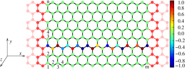
Figure 1: (Color online). Schematic illustration of a two-terminal ZGNR with a line-disorder. The disorder sites are denoted by random colors chosen from the color bar given at the right side of the geometry. The different colors indicate the value of the random on-site potentials at the carbon atoms, and are taken from a rectangular random distribution between $[-1:1]$. Rest of the carbon atoms have the same on-site potential (zero) denoted by the green color. The left and right leads are represented by the red color.

The Rashba SO interaction is assumed to be present in the central scattering region only, while the leads are free from any kind of SO interaction and disorder. Along the $x$-direction, the system has a zigzag shape and along the $y$-direction it has the structure of an armchair, and hence the system is conventionally defined as mZ-nA.

The tight-binding Hamiltonian modeled on a ZGNR in presence of Rashba SO interaction can be written as [54, 55],

$$H=\sum\limits_{i}\epsilon_{i}c_{i}^{\dagger}c_{i}-t\sum\limits_{\langle ij\rangle}c_{i}^{\dagger}c_{j}+i\alpha\sum\limits_{\langle ij\rangle}c_{i}^{\dagger}\left(\vec{\sigma}\times{\bf\hat{d}}_{ij}\right)_{z}c_{j}$$ (1)

where $\epsilon_{i}$ stands for the random on-site potential at the $i$-th carbon atom chosen from a uniform rectangular distribution ($-W$ to $W$). $c_{i}^{\dagger}=\left(c_{i\uparrow}^{\dagger}\quad c_{i\downarrow}^{\dagger}\right)$. $c_{i\sigma}^{\dagger}$ $(\sigma=\uparrow,\downarrow)$ is the creation operator of an electron at site $i$ with spin $\sigma$. The second term is the nearest-neighbor hopping (NNH) term. For simplicity, we assume that the hopping strength between ordered-ordered, ordered-disordered and disordered-disordered carbon atoms has the same value, and that is, $t$. The third term is the nearest-neighbor Rashba term which explicitly violates $z\rightarrow-z$ symmetry. $\vec{\sigma}$ denotes the Pauli spin matrices and $\alpha$ is the strength of the Rashba SO interaction. ${\bf\hat{d}}_{ij}$ is the unit vector that connects the nearest-neighbor sites $i$ and $j$.

The total transmission coefficient, $T$ can be calculated via [56, 57, 58],

$$T=\text{Tr}\left[\Gamma_{L}{\cal G}_{R}\Gamma_{R}{\cal G}_{A}\right]$$ (2)

where ${\cal G}_{R(A)}$ is the retarded (advance) Green’s function. $\Gamma_{L(R)}$ are the coupling matrices representing the coupling between the central region and the left (right) lead. Also, the spin-polarized transmission coefficient $P_{\alpha}$ can be calculated from the relation [59],

$$P_{\alpha}=\text{Tr}\left[\hat{\sigma}_{\alpha}\Gamma_{L}{\cal G}_{R}\Gamma_{R}{\cal G}_{A}\right]/T$$ (3)

where, $\alpha=x,y,z$ and $\sigma$ denote the Pauli matrices, and $T$ as given in Eq. 2.

3 Numerical Results and discussion

We set the hopping term $t=2.7\,$eV [2]. All the energies are measured in units of $t$. The strength of Rashba coupling is fixed at a value given by $\alpha=0.1$, which is very close to the experimentally realized data [28]. The dimension of the scattering region in this work is taken as 241Z-40A. The widths of left and right leads are same as that of the central scattering region. For most of our numerical calculations, we have used KWANT [60].

We have essentially studied the behavior of total transmission $T$ and all the three components of the spin-polarized transmission $P_{\alpha}$ of a ZGNR with line-disorder in presence of Rashba SO interaction. All the results obtained below are averaged over $500$ distinct disordered configurations.

3.1 Total transmission

To begin with, we study the effect of a single line-disorder located at the edges of the ZGNR, specifically, at the top edge or the bottom edge. Subsequently, we study the cases with a number of such disorder lines, where half of the central scattering region is disordered and compare the results with that of a bulk disordered ZGNR.

Figure 2(a) shows the behavior of the transmission coefficient as a function of the Fermi energy in presence of edge-disorder cases. The line-disorder is located at either one of the edges of the ZGNR, that is at the top (green line) or the bottom (black line) edge. The disorder strength is fixed at $W=0.5$. The transmission coefficient is symmetric about $E=0$ and shows identical behavior for the two different edge-disorder cases. Thus, the electronic charges do not feel any difference whether the line-disorder is located at the top or at the bottom edge of the sample. This is owing to the fact that the elements of the $S$-matrix have certain symmetries owing to the geometry of the sample, that is the reflection symmetry $y\rightarrow-y$ [61]. Further, the transmission coefficient exhibits a peculiar behavior as a function of the disorder strength $W$ as shown in Fig. 2(b). For the Fermi energy fixed at a value $E=-0.18$, corresponding to both the top and bottom edge-disorder cases, $T$ shows similar behavior as already seen in Fig. 2(a). For the lower values of disorder, electrons tend to localize, and as a result $T$ decreases. Beyond a certain critical value of $W$, $T$ increases as we increase the disorder strength. It is clear that the delocalization or the extended states emerge in the strong disorder regime.

In order to study the effect of the location of the line-disorder, we have plotted the transmission coefficient as a function of the position of the line-disorder as shown in Fig. 2(c). The Fermi energy is fixed at $E=-0.18$ and the disorder strength is $W=0.5$. The location of the line is governed by the definition of the width of the ZGNR as mentioned earlier. A (zigzag) line-disorder moves from the bottom of the sample to the top, the location of the line number is given in units of $n$ (see Fig. 1). $T$ is symmetric about $n=20$ (width being 40A), where a reflection symmetry exists along $y$-direction.

A comparison between a bulk disordered ZGNR and a set of line-disorder systems has been studied in Fig. 2(d). As mentioned earlier, the width of the ZGNR is 40A, that is we have a total 40 zigzag lines. The set of line-disorder samples are taken as follows. We have considered a single zigzag line, and twenty consecutive zigzag lines from the bottom (half of the ZGNR width).

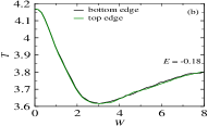
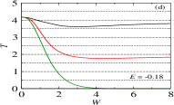
Figure 2: (Color online). (a) Total transmission coefficient $T$ as a function of the Fermi energy for the edge-disorder cases with disorder strength $W=0.5$, where the bottom and top edge disordered cases are denoted by the black and green lines, respectively. (b) $T$ as a function of the strength of disorder for the edge-disorder cases at a typical energy $E=-0.18$, where two different colored curves represent the identical meaning as given in (a). (c) Dependence of total transmission probability on the position of the disorder line ($n$) for $E=-0.18$ and $W=0.5$. (d) $T$-$W$ characteristics at some typical disordered cases where the total number of disordered lines are different. Three distinct cases are shown where the disorder is introduced at the bottom edge, twenty consecutive zigzag lines from the bottom (half of the ZGNR width), and, all over the central scattering region. The corresponding results are denoted by the black, red and green lines, respectively. Here also we choose $E=-0.18$.

For convenience we call these as partially disordered cases. The corresponding transmission coefficients are denoted by black, and red colors respectively. The bulk disorder case is denoted by green color. The complete localization takes place around $W\sim 4$ for the bulk disorder case, which is the familiar Anderson localization. For the partially disordered cases, the scenario is completely different as evident from Fig. 2(b). Moreover, if we look at the strong disorder regime and follow the horizontal dashed lines (drawn to illustrate the slope of $T$), where $T$ increases with $W$, the rate of enhancement of $T$ is greater for the single line-disorder than the half (set of 20 line-disorder) disordered case. Though the localization/delocalization effect has already been discussed in a few recent papers [53, 62, 63] for various kinds of systems, still we have included this feature for the sake of completeness and rigour. Zhong and Stocks [53] had given a proof for this which goes on to explain the anomalous behavior of $T$ in the following way. We may assume that for the partially disordered case, the disordered region is coupled with the rest of the clean (free from disorder but Rashba SO is present) region. If we assume that there is no coupling between these two regions, then there will be localized states in the disordered region, while in the clean region the states will be extended.

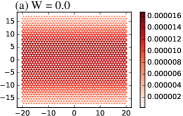
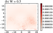
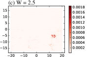
Figure 3: (Color online). LDOS plot for the half disorder ZGNR with (a) $W=0.0$, (b) $W=0.5$, (c) $W=2.5$ and (d) $W=10.0$.

Now suppose we switch on the coupling, which in this case will be the hopping parameter $t$, then there will a competition between the localized states and the extended states associated with the disordered and clean regions, respectively. In the weak disorder regime, the coupling effect is strong, and thus, the localized states will affect the electron transport more than that by the extended states, resulting reduced transmission probability with $W$ in the limit of weak disorder. On the other hand, the coupling effect gradually decreases in the strong disorder regime, where the extended states are less affected by the localized states and as a result, in this limit, the transmission probability increases with increasing disorder.

The anomalous behaviour mentioned above can also be understood from Fig. 3, where we have plotted the space-resolved density of states (LDOS) for three different strengths of disorder, including the disorder-free case. The partially disordered system is considered as half-disorder ZGNR in this case. In the absence of disorder, the LDOS plot (Fig. 3(a)) clearly shows that all the states behave like extended states. Now, for $W=0.5$, the localization starts to occur in the disordered region (Fig. 3(b)). When the disorder strength is $W=2.5$ (close to the critical value, Fig. 3(c)), only a few states have non-zero LDOS, while the amplitude of other states are vanishingly small. This complete localization explains the minimum of the transmission, $T$. Again, for a higher value of disorder, namely $W=10$, there is a complete order-disorder phase separation as seen from Fig. 3(d). At this higher value of $W$, all the states with non-zero amplitudes are located in the disorder-free region, while no such states exist in the disordered region. This discussion also clarifies the distinction between ‘weak’ and ‘strong’ disorder regimes. When the disorder strength is less than the critical value, where the electronic states behave like extended states, we call this regime as weak, and beyond the critical value, the regime is strong disorder regime.

3.2 Spin-polarized transmission

So far, we have studied the total transmission probability for a variety of line-disorder scenarios as well as for the bulk disordered case in presence of Rashba SO interaction. Let us now study the characteristic features of the spin-polarized transmission which is the central focus of our work. In a pristine GNR,

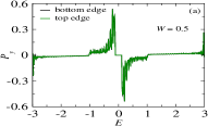
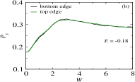
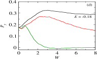
Figure 4: (Color online). The $y$-component of spin-polarized transmission ($P_{y}$) under different conditions. (a) $P_{y}$ as a function of the Fermi energy for the edge-disorder cases setting $W=0.5$. (b) $P_{y}$-$W$ characteristics for the edge-disorder cases. (c) Dependence of $P_{y}$ on the position of the line-disorder ($n$). Here we choose $W=0.5$. (d) $P_{y}$ as a function of $W$ for some distinct disordered cases, where different colors represent the identical meaning as described in Fig. 2(d). In the spectra (b)-(d) we choose $E=-0.18$.

one can have only the $y$-component of the spin-polarized transmission due to the longitudinal mirror symmetry of the finite width GNR in presence of Rashba SO interaction. However, the inclusion of line(s) disorder destroys this symmetry, and as a result, the other two components, namely, $P_{x}$ and $P_{z}$ start contributing in addition to $P_{y}$ [64].

The characteristic features of $P_{y}$ are shown in Fig. 4. In Fig. 4(a), $P_{y}$ is plotted as a function of the Fermi energy for the disorder strength $W=0.5$. The behavior of $P_{y}$ for the top and bottom line-disorder cases are identical and this feature is similar to that of the total transmission coefficient as shown in Fig. 2. However, $P_{y}$ as a function of the disorder strength shows completely different behavior that of the charge transmission $T$ (Fig. 4(b)), that is, starting with a non-zero value ($P_{y}\sim 0.18$ at $W=0$), $P_{y}$ increases (along the positive direction i.e., suppressing down spin propagation) up to a certain disorder strength $W\sim 3.0$ (below this value the Anderson localization dominates, as observed from Fig. 3), and then slowly decreases with increasing $W$. This behavior is peculiar as it implies that the Anderson localization is beneficial to the spin-polarized transport for line-disorder ZGNR.

Moreover, as mentioned earlier that due to the finite width of the ZGNR the longitudinal mirror symmetry is broken along the $y$-axis, even when $W=0$, which results a non-zero $P_{y}$. When we introduce edge-disorder, the system acquires another asymmetric feature, which in turn aids $P_{y}$ even in the presence of Anderson localization. The variation of $P_{y}$ as a function of the location of the line-disorder is shown in Fig. 4(c). It is symmetric about $n=20$. The different line-disorder scenarios are shown in Fig. 4(d) and

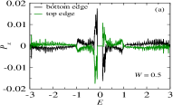
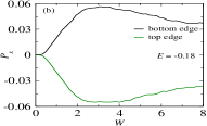
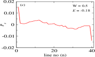
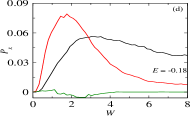
Figure 5: (Color online). The $x$-component of spin-polarized transmission ($P_{x}$) under same different conditions as described in four spectra of Fig. 4.

colors have the same meaning as mentioned in the context of Fig. 2(d). For the partially disordered cases, $P_{y}$ increases in the weak disorder regime up to a critical disorder strength. This value of critical disorder is not unique and depends on the number of line-disorder present in the system. $P_{y}$ increases beyond this critical value in the strong disorder regime. For the bulk disorder case (green curve), $P_{y}$ shows similar feature as the partially disordered cases in low disorder regime, whereas in presence of large disorder $P_{y}$ drops nearly to zero for $W>4$ due to almost complete electronic localization.

As the line-disorder is introduced, due to the broken longitudinal mirror symmetry, finite $P_{x}$ and $P_{z}$ are generated. Figure 5 shows the characteristic feature of the $x$-component of the spin-polarized transmission. For the top and bottom line-disorder cases (denoted by green and black colors, respectively), $P_{x}$ is antisymmetric with respect to each other (Fig. 5(a)). $P_{x}$ is also antisymmetric as a function of the Fermi energy about $E=0$. The antisymmetric nature of $P_{x}$ for the top and bottom edge-disorder cases is also due to the same reason as given in Fig. 4(a) for the explanation of the symmetric behavior of $P_{y}$. Figure 5(b) shows the variation of $P_{x}$ as a function of disorder strength $W$ for the top and bottom line-disorder scenarios. At $W=0$, it is expected that $P_{x}$ should be zero due to the longitudinal mirror symmetry along the $x$-axis, but it remains vanishingly small up to very low values of $W$. While the inclusion of weak disorder can destroy the longitudinal mirror symmetry, the localization still dominates in this regime. $P_{x}$ again shoots up with increasing disorder strength, and beyond the critical value $W\sim 3$ (this value has also been noted from the behavior of $T$ and $P_{y}$ for edge-disorder) it decreases with increasing $W$. Moreover, $P_{x}$ has equal magnitude and opposite phases for the top and bottom line-disorder cases, which also make the line-disordered ZGNR not only an efficient spin-filter device, but also a switching device. This feature can also be verified from the variation of $P_{x}$ as a function of the impurity position as shown in Fig. 5(c). Here the phase of $P_{x}$ continuously changes from being positive to negative as we move the impurity position from the bottom edge to the top edge of the ZGNR. Thus, it is possible to tune the magnitude and determine the phase of $P_{x}$ by changing the location of the line-disorder which is undoubtedly an important observation. Finally, the behavior of $P_{x}$ as a function of $W$ for the different disordered cases is shown in Fig. 5(d). For the partially disordered systems, the peculiar behavior (viz, the spin-polarized transmission enhances in presence of weak disorder, while the reverse happens for the strong disorder) is again prominent like what we get in the case of $P_{y}$ (see Fig. 4(d)). For the bulk disorder ZGNR, $P_{x}$ shows vanishingly small amplitude and beyond a certain value of $W$ it completely disappears.

Finally, we have studied the characteristic features of the $z$-component of spin-polarized transmission and the results are shown in Fig. 6. The variation of $P_{z}$ as a function of the Fermi energy shows similar nature (Fig. 6(a)) to that of $P_{x}$. All the spin-polarized components are antisymmetric about $E=0$ as a function of the Fermi energy due to the electron-hole symmetry of the system. For the top and bottom edge-disorder cases,

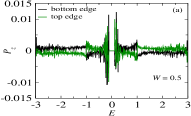
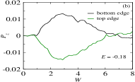
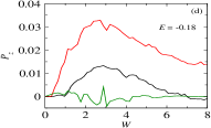
Figure 6: (Color online). The $z$-component of spin-polarized transmission ($P_{x}$) under same different conditions as described in four spectra of Fig. 4.

$P_{z}$ has equal and opposite magnitudes (Fig. 6(b)) indicates the switching property of $P_{z}$ as we have observed in the case of $P_{x}$. As a function of the location of line-disorder, $P_{z}$ is nearly antisymmetric about $n=20$ as shown in Fig. 6(c). The fluctuations in $P_{z}$ are owing to the finite size effects. Figure 6(d) shows the behavior of $P_{z}$ as a function of $W$ for different disorder scenarios. For the half disordered case, the same peculiar behavior is prominent as seen from the behaviour of $P_{x}$ and $P_{y}$ (Fig. 5(d) and Fig. 4(d), respectively). In presence of bulk disorder, $P_{z}$ has very small amplitude, and beyond a certain value of disorder strength, it completely vanishes.

Though the results presented here have been worked out for certain specific parameter values considering a typical system size of the ZGNR, all the physical pictures remain valid

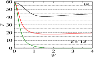
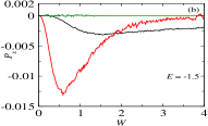
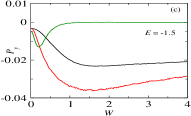
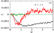
Figure 7: (Color online). (a) $T$, (b) $P_{x}$, (c) $P_{y}$ and (d) $P_{z}$ as a function of $W$ for some distinct disordered cases, where different colors represent the identical meaning as described in Fig. 2(d). The Fermi energy is fixed at $E=-1.5$.

for any other set of parameter values. In support of this, we have also shown a few results corresponding to a different values of the Fermi energy, namely, $E=-1.5$ as shown in Fig. 7. Here, we have shown the behavior of $T$, $P_{x}$, $P_{y}$ and $P_{z}$ as a function of disorder strength $W$. Though the magnitudes of the different spin-polarized components have lower values compared to those for earlier cases, the anomalous behavior is still prominent at this particular energy, which accounts for the robustness of our analysis. Having done a thorough and extensive numerical study, we observe that this feature is also robust for any number of disordered lines in a ZGNR. However they are skipped for the sake of brevity. Moreover, it is also important to note that since the inclusion of the line defect (irrespective of the number of lines), including the bulk disorder, destroys the longitudinal mirror symmetry of the system [64], and hence non-zero $P_{x}$ and $P_{z}$ will always be generated along with $P_{y}$.

4 Experimental perspective

We propose a possible device fabrication technique where a order-disorder structure can be realized. Using the ‘Dip-Pen’ nanolithography (DPN) [67] it is possible to create a selective rough surface. Now, if we manage to create such a surface in one half of the substrate region, while other half is smooth, then the GNR grown on that substrate will acquire the morphology of the substrate. Such substrate morphology can also be achieved using other nanolithography techniques such as photolithgraphy, X-ray lithography with proper masking [68] etc.

All the three components of the spin-polarization can be measured by using a Wien filter and Mott detector (see Ref. [69] for detailed discussion).

5 Conclusion

To summarize, in the present work, we have critically investigated the characteristic features of charge and spin dependent transport properties of zigzag graphene nanoribbons with line(s) of disorder in the presence of Rashba SO interaction within a tight-binding framework based on Green’s function formalism. The disordered region is considered at the edges (top and bottom edges separately), comprising of a few zigzag lines, and, in order to compare the results of these spatially non-uniform disordered ZGNRs with a spatially uniform disordered ZGNR we have considered bulk disordered ZGNR.

The behavior of the charge and spin transport properties for partially disordered scenario show completely contradicting features to that of a bulk disordered ZGNR. The charge transmission decreases in the weak disorder regime due to the Anderson localization, while in the strong disorder regime the extended electronic states dominate and the charge transmission increases with increasing disorder strength, suppressing the effect of electronic localization. All the three components of the spin-polarized transmission ($P_{x}$, $P_{y}$ and $P_{z}$) demonstrate completely inverted behavior to that of the charge transport. Our results predict that for the $y$-component of spin-polarized transmission, the magnitudes and the phases are same for the top and bottom line-disorder cases, while for the $x$ and $z$-components the magnitudes are same but they have opposite phases. The symmetry analysis of the $S$-matrix elements [61, 65, 66] also agrees with our findings. Since the presence of line-disorder can generate all the three components of the spin-polarized transmission, a line-disorder ZGNR can be implemented as an efficient spin-filter device. Moreover, by studying the effect of the location of line impurity, the system can be used to tune the magnitude as well as the phase of $P_{x}$. Since the $x$ and $z$-components have the same magnitude but opposite phases for the top and bottom line-disorder cases, the system can be utilized as a switching device.

References

- [1] K. S. Novoselov et al., Science 306, 666 (2004).
- [2] A. H. C. Neto, F. Guinea, N. M. R. Peres, K. S. Novoselov, and A. K. Geim, Rev. Mod. Phys. 81, 109 (2009).
- [3] Luis E. Hueso et al., Nature 445, 410 (2007).
- [4] N. Tombros, C. Jozsa, M. Popinciuc, H. T. Jonkman and B. J. van Wees, Nature 448, 571 (2007).
- [5] P. J. Zomer, M. H. D. Guimarães, N. Tombros, and B. J. van Wees, Phys. Rev. B 86, 161416(R) (2012).
- [6] T.- Y. Yang et al., Phys. Rev. Lett. 107, 047206 (2011).
- [7] W. Han and R. K. Kawakami, Phys. Rev. Lett. 107, 047207 (2011).
- [8] Y. Zhang, Y.-W. Tan, H. L. Stormer, and P. Kim, Nature 438, 201 (2005).
- [9] V. P. Gusynin and S. G. Sharapov, Phys. Rev. Lett. 95, 146801 (2005).
- [10] E-J. Kan, Z. Li, J. Yang, and J. G. Hou, Appl. Phys. Lett. 91, 243116 (2007).
- [11] X. Lin and J. Ni, Phys. Rev. B 84, 075461 (2011).
- [12] X. Du, I. Skachko, A. Barker, and E. Y. Andrei, Nat. Nanotech. 3 491 (2008).
- [13] K. I. Bolotin, K. J. Sikes, J. Hone, H. L. Stormer, and P. Kim, Phys. Rev. Lett. 101 096802 (2008).
- [14] K. Wakabayashi, M. Fujita, H. Ajiki and M. Sigrist, Phys. Rev. B 59, 8271 (1999).
- [15] R. Saito, M. Fujita, G. Dresselhaus, and M. S. Dresselhaus, Appl. Phys. Lett. 60 , 2204 (1992).
- [16] O. V. Yazyev and M. I. Katsnelson, Phys. Rev. Lett. 100, 047209 (2008).
- [17] O. V. Yazyev, Nano Lett. 8, 1011 (2008).
- [18] G. Cantele, Y.-S. Lee, D. Ninno, and N. Marzari, Nano Lett. 9, 3425 (2009).
- [19] S. A. Wolf et al., Science 294, 5546 (2001).
- [20] Q. F. Sun and X. C. Xie, Phys. Rev. B 71, 155321 (2005).
- [21] Q. F. Sun and X. C. Xie, Phys. Rev. B 73, 235301 (2006).
- [22] F. Chi, J. Zheng, and L. L. Sun, Appl. Phys. Lett. 92, 172104 (2008).
- [23] M. Dey, S. K. Maiti, and S. N. Karmakar, J. Appl. Phys. 109, 024304 (2011).
- [24] S. K. Maiti, Phys. Lett. A 379, 361 (2015).
- [25] S. Sil, S. K. Maiti, and A. Chakrabarti, J. Appl. Phys. 112, 024321 (2012).
- [26] M. Gmitra, S. Konschuh, C. Ertler, C. Ambrosch-Draxl, and J. Fabian, Phys. Rev. B 80, 235431 (2009).
- [27] M. Gmitra, D. Kochan, P. Högl, and J. Fabian, Phys. Rev. B 93, 155104 (2016).
- [28] Y. S. Dedkov, M. Fonin, U. Rüdiger, and C. Laubschat, Phys. Rev. Lett. 100, 107602 (2008).
- [29] F. Calleja et al., Nature Phys. 11, 43 (2015).
- [30] Z. F. Wang, Q. Li, H. Zheng, H. Ren, H. Su, Q. W. Shi, and J. Chen, Phys. Rev. B 75, 113406 (2007).
- [31] Y. Ouyang, S. Sanvito, and J. Guo, Surf. Sci. 605, 1643 (2011).
- [32] B. Huang, Phys. Lett. A 375, 845 (2011).
- [33] G. P. Tang, J. C. Zhou, Z. H. Zhang, X. Q. Deng, and Z. Q. Fan, Appl. Phys. Lett. 101, 023104 (2012).
- [34] K. V. Bets and B. I. Yakobson, Nano Res, 2, 161 (2009).
- [35] S. H. R. Sena, J. M. Pereira Jr., G. A. Farias, F. M. Peeters, and R. N. Costa Filho, J. Phys.: Condens. Matter 24, 375301 (2012).
- [36] C. P. Chang, B. R. Wu, R. B. Chen, and M. F. Lin, J. Appl. Phys. 101, 063506 (2007).
- [37] Y. Park, G. Kim, and Y. H. Lee, Appl. Phys. Lett. 92, 083108 (2008).
- [38] Yun Ren and Ke-Qiu Chen, J. Appl. Phys. 107, 044514 (2010).
- [39] C. Weeks, J. Hu, J. Alicea, M. Franz, and R. Wu, Phys. Rev. X 1, 021001 (2011).
- [40] S. Ganguly and S. Basu, Mater. Res. Express 4, 11 (2017).
- [41] J. Y. Yan, P. Zhang, B. Sun, H. Z. Lu, Z. G. Wang, S. Q. Duan, and X. G. Zhao, Phys. Rev. B 79, 115403 (2009).
- [42] H. Şahin and R. T. Senger, Phys. Rev. B 78, 205423 (2008).
- [43] M. Topsakal, E. Aktürk, H. Sevinçli, and S. Ciraci, Phys. Rev. B 78, 235435 (2008).
- [44] N. M. R. Peres, F. D. Klironomos, S. W. Tsai, J. R. Santos, J. M. B. Lopes dos Santos, and A. H. Castro Neto, Europhys. Lett. 80, 67007 (2007).
- [45] J. Lahiri, Y. Lin, P. Bozkurt, I. I. Oleynik, and M. Batzill, Nature Nanotechnol. 5, 326 (2010).
- [46] X. Lin and J. Ni, Phys. Rev. B 84, 075461 (2011).
- [47] S. Okada, T. Kawai, and K. Nakada, J. Phys. Soc. Jpn. 80, 013709 (2011).
- [48] D. Gunlycke and C. T. White, Phys. Rev. Lett. 106, 136806 (2011).
- [49] R. N. Costa Filho, G. A. Farias, and F. M. Peeters, Phys. Rev. B 76, 193409 (2007).
- [50] P. Dutta, S. K. Maiti, and S. N. Karmakar, J. Appl. Phys. 114, 034306 (2013).
- [51] W. Long, Q. F. Sun, and J. Wang, Phys. Rev. Lett. 101, 166806 (2008).
- [52] J. Wurm, M. Wimmer, and K. Richter, Phys. Rev. B 85, 245418 (2012).
- [53] J. Zhong and G. M. Stocks, Nano Lett. 6, 128 (2006).
- [54] C. L. Kane and E. J. Mele, Phys. Rev. Lett. 95, 226801 (2005).
- [55] C. L. Kane and E. J. Mele, Phys. Rev. Lett. 95, 146802 (2005).
- [56] C. Caroli, R. Combescot, P. Nozieres, and D. Saint-James, J. Phys C: Solid State Phys. 4, 916, (1971).
- [57] D. S. Fisher and P. A. Lee, Phys. Rev. B 23, 6851 (1981).
- [58] S. Datta, Electronic transport in mesoscopic systems, Cambridge University Press, Cambridge (1995).
- [59] P.-H. Chang, F. Mahfouzi, N. Nagaosa, and B. K. Nikolic, Phys. Rev. B 89, 195418 (2014).
- [60] C. W. Groth, M. Wimmer, A. R. Akhmerov, and X. Waintal, New J. Phys. 16, 063065 (2014).
- [61] A. A. Kiselev and K. W. Kim, J. Appl. Phys. 94, 4001 (2003).
- [62] S. K. Maiti, Chem. Phys. Lett. 446, 4 (2007).
- [63] C. Y. Yang, J. W. Dinga, and N. Xu, Physica B 394, 69 (2007).
- [64] L. Chico, A. Latge, and L. Brey, Phys. Chem. Chem. Phys. 17, 16469 (2015).
- [65] M. Dey, S. K. Maiti, S. Sil, and S. N. Karmakar, J. Appl. Phys. 114, 164318 (2013).
- [66] S. Ganguly, S. Basu, and S. K. Maiti, Superlattices and Microstruct. 120, 650 (2018).
- [67] R. D. Piner, J. Zhu, F. Xu, S. Hong, and C. A. Mirkin, Science 283, 661 (1999).
- [68] C. Acikgoz, M. A. Hempenius, J. Huskens, and G. J. Vancso, European Polymer Journal 47, 2033 (2011).
- [69] E. Kisker, Review of Scientific Instruments 53, 507 (1982).