On the Structure of Higher Order Voronoi Cells

Abstract

The classic Voronoi cells can be generalized to a higher-order version by considering the cells of points for which a given $k$-element subset of the set of sites consists of the $k$ closest sites. We study the structure of the $k$-order Voronoi cells and illustrate our theoretical findings with a case study of two-dimensional higher-order Voronoi cells for four points.

1 Introduction

The classic Voronoi cells partition the Euclidean space into polyhedral regions that consist of points nearest to one of the sites from a given finite set. We consider higher order (or multipoint) Voronoi cells that correspond to the subsets of points nearest to $k$ several sites (see an illustration in Fig. 1).

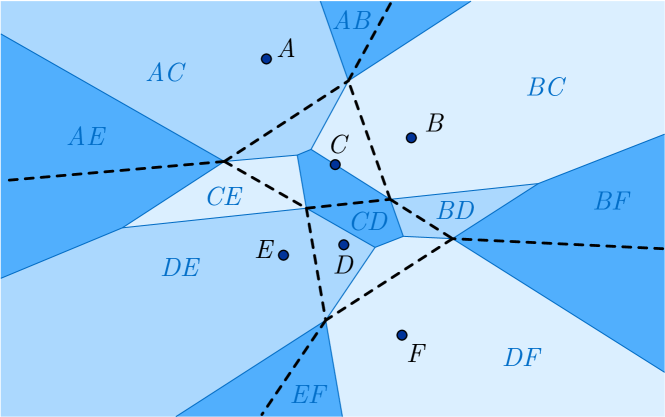
Figure 1: The classic and order two Voronoi diagrams on six sites (shown in dashed lines and shaded regions, respectively). Notice that some two-point combinations generate empty cells.

To our best knowledge, the earliest mention of $k$-point Voronoi cells appears in [1], where a tessellation of the plane by such cells was called the Voronoi diagram of order $k$; that paper also provides bounds on the number of nonempty cells in a plane and complexity estimates for the construction of such diagrams; in [2] the complexity of constructing the higher-order diagrams for line segments was studied.

The multipoint or $k$-order Voronoi diagrams discussed in this paper are one possible way to generalize the classic construction. Some notable generalizations are the cells of more general sets [2, 3], the use of non-Euclidean metrics [4, 5, 6] and the abstract cells that are defined via manifold partitions of the space rather than distance relations [7].

Much of the recent work mentioned above is focussed on the algorithmic complexity of constructing planar Voronoi diagrams of various types. In this paper we rather focus on the structure of multipoint Voronoi cells, and in particular obtain constructive characterizations of cells with nonempty interior, also of bounded and empty cells. We use these results for a case study of multipoint cells defined on at most four sites. We prove that—perhaps counterintuitively—some convex polygons, including triangles and cyclic quadrilaterals, can not be such cells, and provide explicit algorithms for the construction of sites for a given cell in other cases.

Finally, we would like to mention a wealth of emerging application of higher order Voronoi cells, predominantly driven by the recent advancements in big data and mobile sensor technology. For instance, in [8] such cells are utilized in a numerical technique for smoothing point clouds from experimental data; in [9] $k$-order cells are used for detecting and rectifying coverage problems in wireless sensor networks; in [10] the $k$-order diagrams are used to analyze coalitions in the US supreme court voting decisions. A well-known application of the higher order Voronoi cells is in a $k$-nearest neighbor problem in spatial networks [11], however, the practical implementations are limited due to the complexity of higher order diagrams and the lack of readily available software.

Our work is organized as follows. In Section 2 we study the structure of higher order Voronoi cells, and in particular prove the conditions for the cell to be bounded and nonempty. In Section 3 we study the special case of higher order cells on no more than four sites. We will refer to the higher order cells as multipoint cells, to highlight the discrete nature of our construction.

2 High Order Voronoi Cells in $\mathbb{R}^{n}$

Let $T\subset\mathbb{R}^{n}$ be finite and nonempty. For a nonempty proper subset $S\subset T$ we define the multipoint Voronoi cell as the set of points that are not farther from each point of $S$ than from each point of $T\setminus S$,

$$V_{T}(S):=\left\{x\in\mathbb{R}^{n}\,:\,\max_{s\in S}\operatorname{dist}(s,x)\leq\min_{t\in T\setminus S}\operatorname{dist}(t,x)\right\},$$

where $\operatorname{dist}(x,y)$ is the Euclidean distance function. When $S$ is a singleton, i.e. $S=\{s\}$, the set $V_{T}(S)$ is a classic Voronoi cell. We abuse the notation slightly and write $V_{T}(s):=V_{T}(\{s\})$. It is evident that

$$V_{T}(S)=\bigcap_{s\in S}V_{\{s\}\cup\left(T\setminus S\right)}(s).$$ (1)

It is not difficult to observe that each multipoint Voronoi cell is a convex polyhedron, i.e. the intersection of finitely many closed halfspaces, since each cell is defined by finitely many linear inequalities. Explicitly, we have the following representation.

Proposition 2.1.

Let $T$ be a finite subset of $\mathbb{R}^{n}$, and let $S$ be a nonempty and proper subset of $T$. Then $V_{T}\left(S\right)$ is the intersection of $|S|(|T|-|S|)$ closed halfspaces:

$$V_{T}(S)=\bigcap_{\begin{subarray}{c}s\in S\\ t\in T\setminus S\end{subarray}}\left\{x\in\mathbb{R}^{n}\,:\,\langle t-s,x\rangle\leq\frac{1}{2}\left(\|t\|^{2}-\|s\|^{2}\right)\right\}.$$ (2)

Proof.

Observe that, from the definition,

$$V_{T}(S) =\left\{x\in\mathbb{R}^{n}\,:\,\max_{s\in S}\operatorname{dist}(x,s)\leq\min_{t\in T\setminus S}\operatorname{dist}(x,t)\right\}$$

$$=\bigcap_{s\in S}\left\{x\in\mathbb{R}^{n}\,:\,\operatorname{dist}(x,s)\leq\min_{t\in T\setminus S}\operatorname{dist}(x,t)\right\}$$

$$=\bigcap_{s\in S}\bigcap_{t\in T\setminus S}\left\{x\in\mathbb{R}^{n}\,:\,\operatorname{dist}(x,s)\leq\operatorname{dist}(x,t)\right\}.$$

Explicitly for the Euclidean distance function we have

$$\operatorname{dist}(x,s)\leq\operatorname{dist}(x,t)\quad\Leftrightarrow\quad\|x\|^{2}-2\langle s,x\rangle+\|s\|^{2}\leq\|x\|^{2}-2\langle t,x\rangle+\|t\|^{2},$$ (3)

from where the desired representation follows. ∎

As a consequence of a well known necessary and sufficient condition for the inconsistency of an arbitrary system of linear inequalities [12, Theorem 4.4(i)], from (2) we obtain the following characterization of empty Voronoi cells.

Theorem 2.1.

Let $T$ be a finite subset of $\mathbb{R}^{n}$, and let $S$ be a nonempty and proper subset of $T$. Then

$$V_{T}(S)=\emptyset$$

iff

$$\begin{pmatrix}0_{n}\\ -1\end{pmatrix}\in\operatorname{cone}\left\{\begin{pmatrix}t-s\\ \|t\|^{2}-\|s\|^{2}\end{pmatrix},\;s\in S,\,t\in T\setminus S\right\}.$$ (4)

We use the characterization in Theorem 2.1 to obtain two well known statements about the classic Voronoi cells.

Corollary 2.1.

Let $T$ be a finite subset of $\mathbb{R}^{n}$ with $|T|\geq 2.$ Then

$$V_{T}(T\setminus\{t\})\neq\emptyset$$

iff $t$ is an extreme point (vertex) of $\operatorname{conv}T$.

Proof.

Suppose that there exists $s\in T$ such that $V_{T}\left(s\right)=\emptyset.$ Then (4) holds for $S=\{s\}$, and therefore there exist $\lambda_{t}\geq 0$ for $t\in T\setminus\{s\}$ such that

$$\sum_{t\in T\setminus\{s\}}\lambda_{t}\left(t-s\right)=0_{n}\quad\text{ and }\quad\sum_{t\in T\setminus\{s\}}\lambda_{t}\left(\|t\|^{2}-\|s\|^{2}\right)=-1,$$

whereby

$$\lambda_{0}:=\sum_{t\in T\setminus\{s\}}\lambda_{t}>0\;\text{ and }\;s=\sum_{t\in T\setminus\{s\}}\frac{\lambda_{t}}{\lambda_{0}}t.$$

Since the the square of the Euclidean norm $\left\|.\right\|^{2}$ is a strictly convex function, we have

$$\sum_{t\in T\setminus\{s\}}\lambda_{t}\left\|t\right\|^{2}+1 =\sum_{r\in T\setminus\{s\}}\lambda_{r}\left\|s\right\|^{2}=\lambda_{0}\left\|s\right\|^{2}<\lambda_{0}\sum_{t\in T\setminus\{s\}}\frac{\lambda_{t}}{\lambda_{0}}\|t\|^{2}$$

$$=\sum_{t\in T\setminus\{s\}}\lambda_{t}\left\|t\right\|^{2},$$

which is a contradiction. Now, suppose that $V_{T}(T\setminus\{t\})=\emptyset$. Denote $S:=T\setminus\{t\}$. From Theorem 2.1, there exist $\lambda_{s}\geq 0$ for $s\in S$ such that

$$\sum_{s\in S}\lambda_{s}\left(t-s\right)=0_{n}\;\text{ and }\;\sum_{s\in S}\lambda_{s}\left(\left\|t\right\|^{2}-\left\|s\right\|^{2}\right)=-1,$$

whereby

$$\sum_{s\in S}\lambda_{s}>0\;\text{ and }\;t=\sum_{s\in S}\frac{\lambda_{s}}{\sum_{r\in S}\lambda_{r}}s.$$

Hence, $t$ is not an extreme point. If $t$ is not an extreme point, then there exist $\lambda_{s}\geq 0,$ $s\in S$ with $\sum_{s\in S}\lambda_{s}=1$ and $t=\sum_{s\in S}\lambda_{s}s.$ Since $\left\|.\right\|^{2}$ is a strictly convex function,

$$\left\|t\right\|^{2} <\sum_{s\in S}\lambda_{s}\|s\|^{2};$$

therefore, setting $\mu_{s}:=\frac{\lambda_{s}}{\sum_{r\in S}\lambda_{r}\|r\|^{2}-\left\|t\right\|^{2}}$ for $s\in S$, we have $\mu_{s}\geq 0$,

$$\sum_{s\in S}\mu_{s}\left(t-s\right)=0_{n}\;\text{ and }\;\sum_{s\in S}\mu_{s}\left(\left\|t\right\|^{2}-\left\|s\right\|^{2}\right)=-1,$$

showing that (4) holds, which, in view of Theorem 2.1, proves the corollary. ∎

The following result generalizes the “if” statement in the last part of Corollary 2.1.

Corollary 2.2.

Let $T$ be a finite subset of $\mathbb{R}^{n}$, and let $S$ be a nonempty and proper subset of $T$. If $(\operatorname{conv}S)\cap(T\setminus S)\neq\emptyset$, then $V_{T}(S)=\emptyset$.

Proof.

Taking $t\in(\operatorname{conv}S)\cap(T\setminus S),$ since $t$ is not an extreme point of $\operatorname{conv}S,$ by Corollary 2.1 we have $V_{T}(S)\subseteq V_{S\cup\left\{t\right\}}(S)=\emptyset.$ ∎

In fact we can prove a more general geometric statement which yields the preceding corollary.

Theorem 2.2.

Let $T$ be a finite subset of $\mathbb{R}^{n}$, and let $S$ be a nonempty and proper subset of $T$. Then

$$V_{T}(S)\neq\emptyset$$

iff there exists a closed Euclidean ball $B\supset S$ such that

$$\operatorname{int}B\cap(T\setminus S)=\emptyset.$$

Proof.

First assume that $V_{T}(S)\neq\emptyset$. Then there exists $c\in V_{T}(S)$. Let

$$R:=\max_{s\in S}\operatorname{dist}(c,s),$$

and let $B$ be the closed Euclidean ball of radius $R$ centered at $c,$ clearly $S\subset B$. Evidently, $\operatorname{int}B\cap(T\setminus S)=\emptyset$, otherwise we would have $\operatorname{dist}(c,t)<\operatorname{dist}(c,s)$ for some $t\in T\setminus S$ and $s\in S$, hence, $c\notin V_{T}(S)$, which contradicts our choice of $c$. Now assume that there exists some closed Euclidean ball $B$ such that $S\subset B$ and $\operatorname{int}B\cap(T\setminus S)=\emptyset$. The centre of the ball $B$ is contained in $V_{T}(S)$, hence, $V_{T}(S)\neq\emptyset$. ∎

We give an explicit example of an empty cell with $|S|=2$ and $|T|=3$.

Example 2.1.

Let $s_{1}=(-1,0)$, $s_{2}=(1,0)$, $t=(0,0)$. It is not difficult to observe that (2) becomes

$$V_{T}(S)=\left\{(x_{1},x_{2})\,:\,x_{1}\leq-\frac{1}{2},x_{1}\geq\frac{1}{2}\right\}=\emptyset.$$

This configuration is shown in Fig. 2.

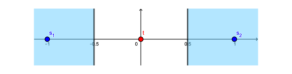
Figure 2: Minimal configuration for an empty cell

Notice that we can likewise construct an empty cell with $|T|>|S|\geq 2$ by making sure that $(T\setminus S)\cap\operatorname{conv}S\neq\emptyset$ (using Corollary 2.2).

Theorem 2.3.

Let $T$ be a finite subset of $\mathbb{R}^{n}$, and let $S$ be a nonempty and proper subset of $T$. Then $V_{T}(S)$ is bounded iff

$$\operatorname{cone}\left\{t-s,s\in S,t\in T\setminus S\right\}=\mathbb{R}^{n}.$$

Proof.

It suffices to observe that from the linear representation (2) we obtain that the first moment cone of $V_{T}(S)$ is $cone\left\{t-s,\;s\in S,t\in T\setminus S\right\}$. ∎

Remark 2.1.

It follows from Theorem 2.3 that if $n\geq 2$ and $|T|\leq 3$ all nonempty cells are unbounded.

We can strengthen the result in the preceding remark as follows.

Theorem 2.4.

Let $T$ be a finite subset of $\mathbb{R}^{n}$. If

$$|T|<2\sqrt{n+1},$$ (5)

then for any $S\subset T$ the cell $V_{T}(S)$ is either empty or unbounded.

Proof.

Assume that $V_{T}(S)=\emptyset.$ The proof is based on the observation that a nonempty bounded polyhedron in $\mathbb{R}^{n}$ must be defined by at least $n+1$ inequalities. Let $p:=|T|$, $k:=|S|$. Then the number of inequalities that feature in the representation (2) is $\phi(k)=k(p-k)$. Observe that $\phi$ attains its maximum at $\frac{p}{2}$ for even $p$ and at $\frac{p-1}{2}$ for odd $p$. Hence for even $p$

$$k(p-k)\leq\frac{p}{2}\left(p-\frac{p}{2}\right)=\frac{p^{2}}{4}=\left\lfloor\frac{p^{2}}{4}\right\rfloor,$$

and for odd $p$

$$k(p-k)\leq\frac{p-1}{2}\left(p-\frac{p-1}{2}\right)=\frac{p^{2}-1}{4}=\left\lfloor\frac{p^{2}}{4}\right\rfloor,$$

hence, ensuring (5) yields at most $n$ inequalities that define each cell, and so all nonempty cells are unbounded. ∎

Proposition 2.2.

Let $S\subset T\subset\mathbb{R}^{n}$, with $|S|=3$ and $|T|=4$. Then $V_{T}(S)$ is either empty or unbounded.

Proof.

Put $T\setminus S=\left\{t\right\}.$ In case $t\in\operatorname{conv}S$, then Corollary 2.1 gives that $V_{T}(S)=\emptyset$. If $t\notin\operatorname{conv}S$, then $t$ can be separated from $S$, and by Theorem 2.3 the cell has to be unbounded. ∎

The following statement will be useful later for a discussion on planar quadrilateral cells.

Proposition 2.3.

Let $S\subset T\subset\mathbb{R}^{2},$ with $S=\{s_{1},s_{2}\}$ and $T\setminus S=\{t_{1},t_{2}\}$. Then

$$V_{T}(S)\text{ is bounded iff }(s_{1},s_{2})\cap(t_{1},t_{2})\text{ is a singleton}.$$

Proof.

The configuration of the points of $T$ in Fig. 3

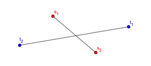
Figure 3: Configuration for a bounded cell

means that if we take the line through $s_{1}$ and $s_{2},$ then $t_{1}$ and $t_{2}$ belong to the two opposite open halfspaces defined by this line. The same holds true if we interchange $s_{1}$ and $s_{2}$ with $t_{1}$ and $t_{2}$. From the linear representation (2) we obtain that the first moment cone $M$ of $V_{T}(S)$ is equal to $\operatorname{cone}\left\{t_{i}-s_{j},\text{ }i,j=1,2\right\}.$ Let us consider that the configuration of the points of $T$ is like in Fig. 3. Then, we are going to prove that $M=\mathbb{R}^{2},$ which, by Theorem 2.3, implies that $V_{T}\left\{S\right\}$ is bounded. What we are actually going to prove is the equivalent assertion that the polar cone $M^{\circ}$ reduces to $\left\{0_{2}\right\}.$ To this aim, let $p\in M^{\circ}$ and assume, w.l.o.g., that $(s_{1},s_{2})\cap(t_{1},t_{2})=\left\{0_{2}\right\}.$ Then there exist $\lambda,\mu>0$ such that $s_{2}=-\lambda s_{1}$ and $t_{2}=-\mu t_{1}.$ Since $\left\langle p,t_{1}-s_{1}\right\rangle\leq 0$ and $\left\langle p,t_{1}+\lambda s_{1}\right\rangle=\left\langle p,t_{1}-s_{2}\right\rangle\leq 0,$ we have $\left\langle p,t_{1}\right\rangle\leq 0.$ This inequality combined with $\left\langle p,-\mu t_{1}-s_{1}\right\rangle=\left\langle p,t_{2}-s_{1}\right\rangle\leq 0$ yields $\left\langle p,s_{1}\right\rangle\geq 0;$ hence, in view of $\left\langle p,-\mu t_{1}+\lambda s_{1}\right\rangle=\left\langle p,t_{2}-s_{2}\right\rangle\leq 0,$ it turns out that $\left\langle p,t_{1}\right\rangle=0=\left\langle p,s_{1}\right\rangle.$ Since $s_{1}$ and $t_{1}$ are linearly independent because of the assumption $(s_{1},s_{2})\cap(t_{1},t_{2})=\left\{0_{2}\right\}$, we conclude that $p=0,$ as was to be proved. Second, let the Voronoi cell $V_{T}\left\{s_{1},s_{2}\right\}$ be bounded. Then, by Theorem 2.3, the first moment cone $\operatorname{cone}\left\{t_{i}-s_{j},\text{ }i,j=1,2\right\}$ is the whole of $\mathbb{R}^{2}.$ This implies that $t_{1}$ and $t_{2}$ are not on a common closed halfplane out of the two determined by the straight line through $s_{1}$ and $s_{2},$ as otherwise that cone would be contained in the translate of that half-space with the boundary line passing through the origin, and the same assertion holds true when we interchange $t_{1}$ and $t_{2}$ with $s_{1}$ and $s_{2}.$ This rules out the possibility that $\operatorname{conv}\left\{s_{1},s_{2},t_{1},t_{2}\right\}$ be a segment, a triangle, or a quadrilateral having $s_{1}$ and $s_{2}$ as adjacent vertices. Therefore $s_{1}$ and $s_{2}$ are opposite vertices of the quadrilateral $\operatorname{conv}\left\{s_{1},s_{2},t_{1},t_{2}\right\},$ which clearly implies that $(s_{1},s_{2})\cap(t_{1},t_{2})$ is a singleton. The proof is completed. ∎

Theorem 2.5.

Let $T$ be a finite subset of $\mathbb{R}^{n}$, and let $S$ be a nonempty and proper subset of $T$. Then

$$\operatorname{int}V_{T}(S)\neq\emptyset$$

iff

$$0_{n+1}\notin\operatorname{conv}\left\{\begin{pmatrix}t-s\\ \left\|t\right\|^{2}-\left\|s\right\|^{2}\end{pmatrix},\quad s\in S,\;t\in T\setminus S\right\}.$$

Proof.

The proof comes from the well known characterization of the Slater condition for a linear system of inequalities [13, Theorem 3.1]. ∎

Example 2.2.

Consider a system $T$ of four points in the plane,

$$T=\{\left(0,0\right),\left(1,1\right),\left(1,0\right),\left(0,1\right)\},\quad S=\{\left(0,0\right),\left(1,1\right)\}.$$

This is illustrated in Fig. 4.

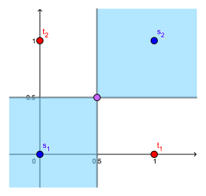
Figure 4: A singleton cell (the intersection of the two shaded regions).

Using Theorems 2.1, 2.3 and 2.5, it is easy to check that $V_{T}\left(S\right)$ is nonempty and bounded, but $\operatorname{int}V_{T}\left(S\right)=\emptyset$. Indeed, $V_{T}\left(S\right)=\left\{\left(\frac{1}{2},\frac{1}{2}\right)\right\}$.

The next statement is a specific characterization for a three-point system, which we will use in what follows.

Proposition 2.4.

Let $T,T^{\prime}\subset\mathbb{R}^{n}$ be such that $|T|=|T^{\prime}|=3$ and $T$ and $T^{\prime}$ differ by exactly one point (i.e. $|T\cap T^{\prime}|=2$). Let $s\in T\setminus T^{\prime}$ and $s^{\prime}\in T^{\prime}\setminus T$. If

$$V_{T}(s)\subseteq V_{T^{\prime}}(s^{\prime}),$$

then all points in the set $T^{\prime}\cup T$ belong to the same straight line.

Proof.

For notational convenience we will prove the result for $T=\{t_{1},t_{2},0\}$ and $T^{\prime}=\{t_{1},t_{2},s\}$, where the points $t_{1},t_{2},s$ are all nonzero and pairwise distinct. Let

$$F:=V_{T}(0)=\left\{x\in\mathbb{R}^{n}\;:\;\langle t_{j},x\rangle\leq\frac{1}{2}\left\|t_{j}\right\|^{2},\;j=1,2\right\},$$

$$F^{\prime}:=V_{T^{\prime}}(s)=\left\{x\in\mathbb{R}^{n}\;:\;\langle t_{j}-s,x\rangle\leq\frac{1}{2}\left(\left\|t_{j}\right\|^{2}-\|s\|^{2}\right),\;j=1,2\right\}.$$

The two inequalities defining $F^{\prime}$ are consequence relations of the inequalities defining $F$. Therefore there exist $\lambda_{ij}\geq 0,$ $i,j=1,2$ such that

$$t_{i}-s=\sum_{j=1}^{2}\lambda_{ij}t_{j},\text{ }i=1,2\text{ and}$$ (6)

$$\left\|t_{i}\right\|^{2}-\left\|s\right\|^{2}\geq\sum_{j=1}^{2}\lambda_{ij}\left\|t_{j}\right\|^{2},\text{ }i=1,2.$$

Hence

$$s=\left(1-\lambda_{ii}\right)t_{i}-\lambda_{i(3-i)}t_{3-i},\text{ }i=1,2\text{ and}$$ (7)

$$\left\|s\right\|^{2}\leq\left(1-\lambda_{ii}\right)\left\|t_{i}\right\|^{2}-\lambda_{i(3-i)}\left\|t_{3-i}\right\|^{2},\text{ }i=1,2.\text{ }$$ (8)

We can subtract the two representations (7) of $s$ to obtain

$$\left(1-\lambda_{11}+\lambda_{21}\right)t_{1}+\left(-1-\lambda_{12}+\lambda_{22}\right)t_{2}=0_{n}.$$

If $t_{j},$ $j=1,2$ are linearly independent, we have

$$1=\lambda_{11}-\lambda_{21}\text{ and }1=\lambda_{22}-\lambda_{12}.$$

Together with (8) this yields

$$0\leq\left\|s\right\|^{2}\leq\left(1-\lambda_{11}\right)\left\|t_{1}\right\|^{2}-\lambda_{12}\left\|t_{2}\right\|^{2}=-\lambda_{21}\left\|t_{1}\right\|^{2}-\lambda_{12}\left\|t_{2}\right\|^{2}\leq 0,$$

which contradicts the condition $s\neq 0$. Therefore $t_{j},$ $j=1,2$ are linearly dependent. Together with (6) this finishes the proof. ∎

Remark 2.2.

This proposition means that it is impossible to enlarge a Voronoi cell of a single point in a three-point affinely independent system by moving this point.

Proposition 2.5.

Let $T$ be a finite subset of $\mathbb{R}^{n}$, and let $S$ be a nonempty proper subset of $T$. If $\left|S\right|\geq 2,$ then

$$V_{T}(S)=\bigcup\limits_{s\in S}\left[V_{T\setminus\{s\}}(S\setminus\{s\})\cap V_{S}(s)\right].$$ (9)

Proof.

Denote

$$A_{s}:=V_{T\setminus\{s\}}(S\setminus\{s\})\cap V_{S}(s).$$

Observe that for any $\bar{s}\in S$ we have

$$A_{\bar{s}}=\{x\in\mathbb{R}^{n}\,:\,\operatorname{dist}(x,\bar{s})\leq\operatorname{dist}(x,s)\leq\operatorname{dist}(x,t)\quad\forall s\in S,\;t\in T\setminus S\}.$$

Evidently, $A_{s}\subseteq V_{T}(S)$ for every $s\in S$, hence, $\bigcup\limits_{s\in S}A_{s}\subseteq V_{T}(S)$. To prove the reverse inclusion, assume that $x\in V_{T}(S)$. Let $\bar{s}$ be a closest point to $x$ in $S$. It is evident that $x\in V_{S}(\bar{s})$. At the same time, it is not difficult to observe that $V_{T}(S)\subseteq V_{T\setminus{\{\bar{s}\}}}(S\setminus\{\bar{s}\})$. Hence

$$x\in V_{T\setminus{\{\bar{s}\}}}(S\setminus\{\bar{s}\})\cap V_{S}(\bar{s})=A_{\bar{s}},$$

and therefore $V_{T}(S)\subseteq\bigcup\limits_{s\in S}A_{s}$. ∎

Proposition 2.6.

Let $T$ be a finite subset of $\mathbb{R}^{n}$, and let $S$ be a nonempty and proper subset of $T$. If there exist $s_{1},s_{2}\in S$ and $t_{1},t_{2}\in T\setminus S$ such that the inequalities

$$\|s_{1}-x\|\leq\|t_{1}-x\|\quad\text{and}\quad\|s_{2}-x\|\leq\|t_{2}-x\|$$ (10)

define the same halfspace, then these inequalities are nonessential for $V_{T}(S)$, i.e. they can be dropped from the system (2).

Proof.

It is evident from the equivalence (3) that these inequalities can be written as

$$\langle t_{1}-s_{1},x\rangle\leq\frac{1}{2}\left(\|t_{1}\|^{2}-\|s_{1}\|^{2}\right),\quad\langle t_{2}-s_{2},x\rangle\leq\frac{1}{2}\left(\|t_{2}\|^{2}-\|s_{2}\|^{2}\right).$$ (11)

If both inequalities in (10) define the same halfspace, then it follows from (11) that there exists $\alpha>0$ such that

$$t_{2}-s_{2}=\alpha(t_{1}-s_{1})\quad\text{and}\quad\frac{1}{2}\left(\|t_{2}\|^{2}-\|s_{2}\|^{2}\right)=\alpha\frac{1}{2}\left(\|t_{1}\|^{2}-\|s_{1}\|^{2}\right).$$ (12)

Every point $x\in V_{T}(S)$ also satisfies the system

$$\langle t_{1}-s_{2},x\rangle\leq\frac{1}{2}\left(\|t_{1}\|^{2}-\|s_{2}\|^{2}\right),\quad\langle t_{2}-s_{1},x\rangle\leq\frac{1}{2}\left(\|t_{2}\|^{2}-\|s_{1}\|^{2}\right).$$ (13)

Adding these inequalities together we obtain

$$\langle t_{1}-s_{2}+t_{2}-s_{1},x\rangle\leq\frac{1}{2}\left(\|t_{1}\|^{2}-\|s_{2}\|^{2}+\|t_{2}\|^{2}-\|s_{1}\|^{2}\right),$$

and using (12) we have a consequence of (13),

$$(1+\alpha)\langle t_{1}-s_{1},x\rangle\leq(1+\alpha)\frac{1}{2}\left(\|t_{1}\|^{2}-\|s_{1}\|^{2}\right),$$

which defines the same halfspace as (11). ∎

Theorem 2.6.

Let $T\subset\mathbb{R}^{n}$ be a finite set, let $S:=\{s_{1},s_{2}\}\subset T$ be a two-point set, and let

$$H :=\{x\in\mathbb{R}^{n}\,:\,\|x-s_{1}\|=\|x-s_{2}\|\}$$

$$=\{x\in\mathbb{R}^{n}\,:\,\langle s_{1}-s_{2},x\rangle=\frac{1}{2}(\|s_{1}\|^{2}-\|s_{2}\|^{2})\}.$$

If $\operatorname{int}V_{T}(S)\neq\emptyset$, then $H\cap\operatorname{ri}F=\emptyset$ for every facet $F$ of $V_{T}(S)$.

Proof.

Let $F$ be the facet of $V_{T}(S)$ defined by the linear equation corresponding to some point $t_{0}\in T$ and, say, $s_{1},$ that is, $\langle t_{0}-s_{1},x\rangle=\frac{1}{2}\left(\|t_{0}\|^{2}-\|s_{1}\|^{2}\right),$ and assume, towards a cotradiction, that $H\cap\operatorname{ri}F\neq\emptyset.$ Take $\overline{x}\in H\cap\operatorname{ri}F.$ We then have

$$\langle t_{0}-s_{1},\overline{x}\rangle=\frac{1}{2}(\|t_{0}\|^{2}-\|s_{1}\|^{2}).$$

Adding the equality

$$\langle s_{1}-s_{2},\overline{x}\rangle=\frac{1}{2}(\|s_{1}\|^{2}-\|s_{2}\|^{2}),$$

which follows from the fact that $\overline{x}\in H,$ to the preceding one, we get

$$\langle t_{0}-s_{2},\overline{x}\rangle=\frac{1}{2}(\|t_{0}\|^{2}-\|s_{2}\|^{2}).$$

Since $\operatorname{int}V_{T}(S)\neq\emptyset$ and $\overline{x}\in\operatorname{ri}F$, there is exactly one halfspace among those defined by the inequalities (2) such that $\overline{x}$ belongs to its boundary hyperplane (and hence to the interior of the remaining halfspaces). Hence the linear equalities

$$\langle t_{0}-s_{1},x\rangle=\frac{1}{2}(\|t_{0}\|^{2}-\|s_{1}\|^{2})$$ (14)

and

$$\langle t_{0}-s_{2},x\rangle=\frac{1}{2}(\|t_{0}\|^{2}-\|s_{2}\|^{2})$$ (15)

define the same hyperplane, which implies the existence of a real number $\lambda$ such that $t_{0}-s_{2}=\lambda\left(t_{0}-s_{1}\right),$ so that the points $t_{0},s_{1},s_{2}$ are colinear. Substituting $x:=\frac{t_{0}+s_{1}}{2},$ which is a solution of (14), into (15) we have, after elementary algebraic manipulation,

$$\langle t_{0}-s_{2},s_{1}-s_{2}\rangle=0,$$

meaning that $s_{1}-s_{2}$ must be orthogonal to $t_{0}-s_{2}$. This, together with the colinearity of $t_{0},s_{1}$ and $s_{2}$ and the fact that these three points ar distinct, yields a contradiction. ∎

3 Case Study

In this section we study the special case of higher order cells on no more than four sites. With the exception of subsections 3.5-3.7, our study will be developed for sets in $\mathbb{R}^{2}.$ For every set $F\subset\mathbb{R}^{2}$ defined by four linear inequalities, we will determine whether or not there exist sets $S\subset T\subset\mathbb{R}^{2},$ with $|S|=2$ and $|T|=4,$ such that $V_{T}(S)=F.$ In the cases when the answer will be affirmative, we will construct the (possibly non necessarity unique) sets $S$ and $T$ explicitly.

3.1 Singletons

A singleton (zero-dimensional) cell $\{c\}$ can be obtained by placing the pairs of points $(s_{1},s_{2})$ and $(t_{1},t_{2})$ in the opposite corners of a square centred at $c$. This was already discussed in Example 2.2. Note that this is a minimal representation, since we need at least three inequalities to obtain a bounded cell (cf. Theorem 2.4), and hence $|T|\geq 4$. In fact the square can be replaced by a rectangle or a general cyclic quadrilateral (we recall that a quadrilateral is said to be cyclic if all of its vertices are on a single circle, which is equivalent to the fact that the sum of opposite angles equals $\pi$).

Proposition 3.1.

Let $S\subset T\subset\mathbb{R}^{2},$ with $|S|=2$ and $|T|=4.$ The following statements are equivalent:

• $V_{T}(S)$ is nonempty and at most one-dimensional.

• The points of $T$ are the vertices of a cyclic quadrilateral, with the two sites of $S$ located opposite to each other (across a diagonal).

• $V_{T}(S)$ is a singleton.

Proof.

Throughout the proof, we use the explicit notation $S:=\{s_{1},s_{2}\}$ and $T:=\{s_{1},s_{2},t_{1},t_{2}\}$. a) $\Rightarrow$ b). Without loss of generality assume that $0\in V_{T}(S)$ while $\operatorname{int}V_{T}(S)=\emptyset$. By Theorem 2.5 we have

$$0=\sum_{i,j\in\{1,2\}}\lambda_{ij}(t_{j}-s_{i}),\qquad 0=\sum_{i,j\in\{1,2\}}\lambda_{ij}(\|t_{j}\|^{2}-\|s_{i}\|^{2}),$$ (16)

where $\lambda_{ij}$ are convex combination coefficients. Since $0\in V_{T}(S)$, we have from (2) that

$$\|t_{j}\|\geq\|s_{i}\|\quad\forall i,j\in\{1,2\}.$$

Without loss of generality assume that

$$\|s_{2}\|\leq\|s_{1}\|\leq\|t_{1}\|\leq\|t_{2}\|.$$

If $\|s_{1}\|<\|t_{1}\|$, then $\|s_{i}\|<\|t_{j}\|$ for all $i,j\in\left\{1,2\right\},$ which implies that the second equality in (16) is impossible. Hence, $\|s_{1}\|=\|t_{1}\|$. If $\|s_{1}\|>\|s_{2}\|$, then $\|t_{i}\|>\|s_{2}\|$ for all $i\in\left\{1,2\right\};$ therefore, from (16), we get $\lambda_{21}=\lambda_{22}=0$ and

$$s_{1}=\lambda_{11}t_{1}+\lambda_{12}t_{2},$$

so $s_{1}\in[t_{1},t_{2}]$ and $\|s_{1}\|^{2}=\lambda_{11}\|t_{1}\|^{2}+\lambda_{12}\|t_{2}\|^{2}$, which holds only when $t_{1}=t_{2}=s_{1}$ by the strict convexity of the squared norm. This is impossible. Likewise, when $\|t_{1}\|<\|t_{2}\|$ we have $\lambda_{12}=\lambda_{22}=0$, then $t_{1}\in[s_{1},s_{2}]$, which by Corollary 2.2 yields $V_{T}(S)=\emptyset$, again a contradiction. We have proved that $\|s_{2}\|=\|s_{1}\|=\|t_{1}\|=\|t_{2}\|$, and hence our sites are the vertices of a cyclic quadrilateral. It is now easy to observe that $s_{1},s_{2}$ are located opposite to each other because, by the first equality in (16), we have $[s_{1},s_{2}]\cap[t_{1},t_{2}]\neq\emptyset$. b) $\Rightarrow$ c) Since the points of $T$ lie on some circle, without loss of generality we may assume that the centre of this circle is the origin, and then $\|t_{1}\|=\|t_{2}\|=\|s_{1}\|=\|s_{2}\|$. In this case the right-hand side of system (2) is zero, and we have, for every point $x\in V_{T}(S),$

$$\langle t_{j}-s_{i},x\rangle\leq 0\quad\forall i,j\in\{1,2\}.$$ (17)

It is evident that $x=0$ is a solution of this system; hence, $V_{T}(S)\neq\emptyset$. On the other hand, from (17) it follows that $V_{T}(S)$ is a cone. From these facts, using Proposition 2.3 we immediately deduce that $V_{T}(S)=\left\{0\right\}.$ The implication c) $\Rightarrow$ a) is obvious. ∎

Note that for the case $|S|=2$ and $|T|=3$ it is impossible to have a nonempty bounded cell due to Remark 2.1. This means that we do not need to consider this configuration when discussing the subsequent cases of bounded polygons.

Furthermore, in the case $|S|=3$ and $|T|=4$ it is impossible to have a bounded cell, as was shown in Proposition 2.2.

Since we have determined that we can not have a nonempty bounded cell for $|T|=|S|+1$, the only possibility to have a singleton cell is for $|S|=2$ and $|T|=4$. Furthermore, we can focus on the latter case when studying other bounded cells.

3.2 One-Dimensional Cells

It follows from the preceding discussion that it is impossible to obtain line segments as multipoint Voronoi cells in our setting.

Corollary 3.1.

Let $S\subset T\subset\mathbb{R}^{2},$ with $|S|=2$ and $|T|=4.$ Then $V_{T}(S)$ is not one-dimensional.

Proof.

Follows directly from Proposition 3.1. ∎

It follows from Corollary 3.1 that it is impossible to have a one-dimensional cell for $|T|=4$, $|S|=2$, so both rays and lines are impossible in this configuration.

Now consider the case $|T|=|S|+1$. If $V_{T}\left(S\right)\neq\emptyset,$ by Corollary 2.2 we must have for $\{t\}=T\setminus S$ that $t\notin\operatorname{conv}S$. By the separation theorem this yields the existence of some $d$, $\|d\|=1$ such that

$$\langle t-s,d\rangle<0\quad\forall s\in S,$$

which yields the existence of a sufficiently small ball $B_{\varepsilon}(d)$ centred at $d$ such that

$$\langle t-s,y\rangle<0\quad\forall s\in S,\;\forall y\in B_{\varepsilon}(d).$$

Then for any $x_{0}\in V_{T}(S)$ and any $y\in B_{\varepsilon}(d)$ we have

$$\langle t-s,x_{0}+y\rangle=\langle t-s,x_{0}\rangle+\langle t-s,y\rangle<\langle t-s,x_{0}\rangle.$$

It is hence clear from the representation in Proposition 2.1 that $x_{0}+B_{\varepsilon}(y)\subset V_{T}(S)$, which gives that $V_{T}(S)$ is one-dimensional.

Thus we have proved the following statement.

Proposition 3.2.

Let $S\subset T\subset\mathbb{R}^{n},$ with $|T|=|S|+1$. Then $V_{T}(S)$ is not one-dimensional.

3.3 Triangles

A somewhat surprising result is that a second order Voronoi cell cannot be a triangle. As discussed previously, we only need to prove this for the case $|S|=2$ and $|T|=4$.

Proposition 3.3.

Let $S\subset T\subset\mathbb{R}^{2},$ with $|S|=2$ and $|T|=4.$ Then $V_{T}(S)$ is not a triangle.

Proof.

Suppose that $V_{T}\left(S\right)$ is a triangle. Denote $T=\{s_{1},s_{2},t_{1},t_{2}\}$, $S=\{s_{1},s_{2}\}$. The cell $V_{T}(S)$ is the solution set of the linear system of inequalities

$$\left\langle c_{ij},x\right\rangle\leq\alpha_{ij}\text{\quad}\left(i,j=1,2\right),$$ (18)

with $c_{ij}:=t_{i}-s_{j}$ and $\alpha_{ij}:=\frac{1}{2}\left(\left\|t_{i}\right\|^{2}-\left\|s_{j}\right\|^{2}\right).$ Notice that

$$\left(\begin{array}[]{c}c_{22}\\ \alpha_{22}\end{array}\right)=-\left(\begin{array}[]{c}c_{11}\\ \alpha_{11}\end{array}\right)+\left(\begin{array}[]{c}c_{12}\\ \alpha_{12}\end{array}\right)+\left(\begin{array}[]{c}c_{21}\\ \alpha_{21}\end{array}\right).$$ (19)

Without loss of generality, we will assume that $0\in\operatorname{int}V_{T}\left(S\right)$, that is, $\alpha_{ij}>0$ $\left(i,j=1,2\right).$ Since (18) defines a triangle, one of its inequalities, say the one corresponding to $i=2=j$ is redundant, so that the triangle is actually the solution set of the system consisting of the other three. We claim that the vectors $\left(\begin{array}[]{c}c_{11}\\ \alpha_{11}\end{array}\right),\left(\begin{array}[]{c}c_{12}\\ \alpha_{12}\end{array}\right)$ and $\left(\begin{array}[]{c}c_{21}\\ \alpha_{21}\end{array}\right)$ are linearly independent. Indeed, assume the existence of $\left(\beta_{11},\beta_{12},\beta_{21}\right)\in\mathbb{R}^{3}\setminus\left\{\left(0,0,0\right)\right\}$ such that

$$\beta_{11}\left(\begin{array}[]{c}c_{11}\\ \alpha_{11}\end{array}\right)+\beta_{12}\left(\begin{array}[]{c}c_{12}\\ \alpha_{12}\end{array}\right)+\beta_{21}\left(\begin{array}[]{c}c_{21}\\ \alpha_{21}\end{array}\right)=\left(\begin{array}[]{c}0_{2}\\ 0\end{array}\right),$$ (20)

and let $\overline{x}$ be the vertex of $V_{T}(S)$ defined by

$$\left\langle c_{12},\overline{x}\right\rangle=\alpha_{12}\text{ and }\left\langle c_{21},\overline{x}\right\rangle=\alpha_{21}.$$ (21)

Then, from (20) and (21) we easily deduce that $\beta_{11}\left(\left\langle c_{11},\overline{x}\right\rangle-\alpha_{11}\right)=0.$ Since $\left\langle c_{11},\overline{x}\right\rangle<\alpha_{11},$ as the three sides of $V_{T}(S)$ don’t have a common point, it follows that $\beta_{11}=0.$ By using the same argument with the other two vertices of $V_{T}(S),$ we deduce that $\beta_{12}=0=\beta_{21},$ thus proving our claim that $\left(\begin{array}[]{c}c_{11}\\ \alpha_{11}\end{array}\right),\left(\begin{array}[]{c}c_{12}\\ \alpha_{12}\end{array}\right)$ and $\left(\begin{array}[]{c}c_{21}\\ \alpha_{21}\end{array}\right)$ are linearly independent. Since the inequality corresponding to $i=2=j$ is redundant, by Farkas’ lemma there exist $\lambda_{ij}\geq 0$ $\left(i,j=1,2\right)$ such that

$$c_{22}=\lambda_{11}c_{11}+\lambda_{12}c_{12}+\lambda_{21}c_{21}\quad\text{and\quad}\alpha_{22}\geq\lambda_{11}\alpha_{11}+\lambda_{12}\alpha_{12}+\lambda_{21}\alpha_{21}.$$ (22)

Considering again the vertex $\overline{x},$ from (19) we obtain that

$$\alpha_{22} =-\alpha_{11}+\alpha_{12}+\alpha_{21}\leq-\left\langle c_{11},\overline{x}\right\rangle+\left\langle c_{12},\overline{x}\right\rangle+\left\langle c_{21},\overline{x}\right\rangle=\left\langle-c_{11}+c_{12}+c_{21},\overline{x}\right\rangle$$

$$=\left\langle c_{22},\overline{x}\right\rangle\leq\alpha_{22};$$

hence, by (22), we deduce that

$$\left\langle c_{22},\overline{x}\right\rangle =\alpha_{22}\geq\lambda_{11}\alpha_{11}+\lambda_{12}\alpha_{12}+\lambda_{21}\alpha_{21}$$

$$\geq\lambda_{11}\left\langle c_{11},\overline{x}\right\rangle+\lambda_{12}\left\langle c_{12},\overline{x}\right\rangle+\lambda_{21}\left\langle c_{21},\overline{x}\right\rangle=\left\langle\lambda_{11}c_{11}+\lambda_{12}c_{12}+\lambda_{21}c_{21},\overline{x}\right\rangle$$

$$=\left\langle c_{22},\overline{x}\right\rangle.$$

Therefore $\lambda_{11}\alpha_{11}+\lambda_{12}\alpha_{12}+\lambda_{21}\alpha_{21}=\alpha_{22},$ that is,

$$\left(\begin{array}[]{c}c_{22}\\ \alpha_{22}\end{array}\right)=\lambda_{11}\left(\begin{array}[]{c}c_{11}\\ \alpha_{11}\end{array}\right)+\lambda_{12}\left(\begin{array}[]{c}c_{12}\\ \alpha_{12}\end{array}\right)+\lambda_{12}\left(\begin{array}[]{c}c_{21}\\ \alpha_{21}\end{array}\right).$$

Comparing this equality with (19) and taking into account that the vectors $\left(\begin{array}[]{c}c_{11}\\ \alpha_{11}\end{array}\right),\left(\begin{array}[]{c}c_{12}\\ \alpha_{12}\end{array}\right)$ and $\left(\begin{array}[]{c}c_{21}\\ \alpha_{21}\end{array}\right)$ are linearly independent, we deduce that $\lambda_{11}=-1,$ a contradiction. ∎

3.4 Bounded Quadrilaterals

We next show that any non-cyclic bounded convex quadrilateral is a second order Voronoi cell with $|T|=4$. We also prove that it is impossible for a cyclic quadrilateral to be a Voronoi cell of 2 points (when $|T|=4$).

Proposition 3.4.

Let $F\subset\mathbb{R}^{2}$ be a non-cyclic bounded convex quadrilateral. Then there exist $S\subset T\subset\mathbb{R}^{2}$, with $|S|=2$ and $|T|=4$, such that $V_{T}(S)=F$.

Proof.

First, looking at Fig. 5, where $F$ is depicted as the quadrilateral $ACBD,$

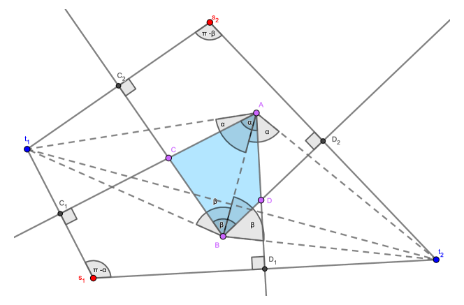
Figure 5: Bounded quadrilateral.

we would like to mention that $\sphericalangle CAD=\alpha>0$ and $\sphericalangle CBD=\beta>0$ and, w.l.o.g., $\pi>\alpha+\beta.$ We draw the lines through $A$ ($B$) that make an angle equal to $\alpha$ (resp., $\beta$) with the segment $AB.$ In this way, we get the points $t_{1}$ and $t_{2}$ as the two other vertices of the quadrilateral having those lines as their sides. We take $s_{1}$ and $s_{2}$ as the symmetric points of $t_{1}$ with respect to the lines $CA$ and $CB,$ respectively, and we set $S:=\left\{s_{1},s_{2}\right\}$ and $T:=\left\{s_{1},s_{2},t_{1},t_{2}\right\}$. The only thing that we have to prove is that $t_{2}s_{1}\bot AD$ and $t_{2}s_{2}\bot BD.$ The point $B$ is the center of the circle passing through the points $t_{1},$ $t_{2}\$and$\ s_{2}.$ Therefore, $\sphericalangle t_{1}s_{2}t_{2}=\pi-\beta,$ which, looking at the quadrilateral $C_{2}s_{2}D_{2}B,$ implies that $t_{2}s_{2}\bot BD.$ The point $A$ is the center of the circle passing through the points $t_{1},$ $t_{2}$ and$\ s_{1}.$ Therefore, $\sphericalangle t_{1}s_{1}t_{2}=\pi-\alpha,$ which, looking at the quadrilateral $C_{1}s_{1}D_{1}A,$ implies $t_{2}s_{1}\bot AD.$ ∎

Observe that the algorithm does not work if $\pi\leq\alpha+\beta$. However it is not difficult to observe that for a non-cyclic convex quadrilateral it is always possible to choose the corners to ensure $\alpha+\beta<\pi$. We have the following negative result.

Proposition 3.5.

Let $S\subset T\subset\mathbb{R}^{2},$ with $|S|=2$ and $|T|=4.$ Then $V_{T}(S)$ is not a cyclic quadrilateral.

Proof.

Assume that the Voronoi cell $V_{T}(S)$ of some set $S:=\{s_{1},s_{2}\}$, with $T:=\{s_{1},s_{2},t_{1},t_{2}\}$, is a cyclic quadrilateral. Then each side of this quadrilateral is defined by the bisector between $s_{i}$ and $t_{j}$ for $i,j\in\{1,2\}$. First, we will show that any two sides defined by the bisectors of disjoint pairs, say, $\{s_{1},t_{1}\}$ and $\{s_{2},t_{2}\}$, cannot be adjoint. Assume the contrary: then without loss of generality the intersection $u$ of the two bisectors is a vertex of $V_{T}(S)$. We have, by using the representation (2),

$$\langle t_{1}-s_{2},u\rangle\leq\frac{1}{2}(\|t_{1}\|^{2}-\|s_{2}\|^{2}),\qquad\langle t_{2}-s_{1},u\rangle\leq\frac{1}{2}(\|t_{2}\|^{2}-\|s_{1}\|^{2}),$$ (23)

and since $u$ is the intersection of the two bisectors,

$$\langle t_{1}-s_{1},u\rangle=\frac{1}{2}(\|t_{1}\|^{2}-\|s_{1}\|^{2}),\qquad\langle t_{2}-s_{2},u\rangle=\frac{1}{2}(\|t_{2}\|^{2}-\|s_{2}\|^{2}).$$ (24)

Adding the two equalities in (24) and rearranging, we obtain

$$\langle t_{1}-s_{2},u\rangle+\langle t_{2}-s_{1},u\rangle=\frac{1}{2}(\|t_{1}\|^{2}-\|s_{2}\|^{2})+\frac{1}{2}(\|t_{2}\|^{2}-\|s_{1}\|^{2}).$$

Together with (23) this yields equalities in (23), and hence the four lines that define the sides of the quadrilateral must intersect at $u$. This is impossible, hence, the assumption is wrong.

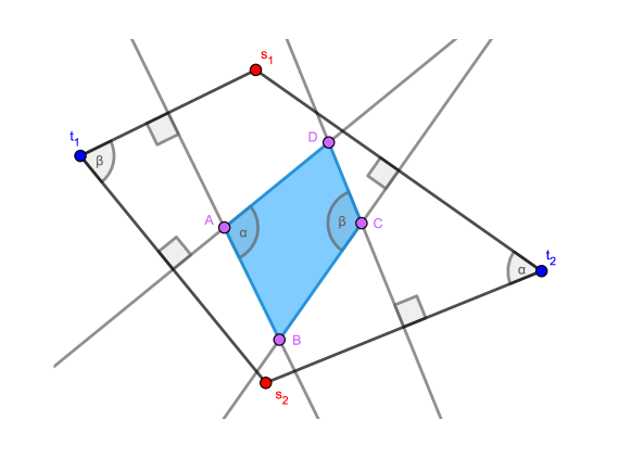
Figure 6: An illustration to the proof of Proposition 3.5.

Now, let us consider the quadrilateral with vertices $s_{1},s_{2},t_{1}$ and $t_{2}.$ Looking at Fig. 6, it is easy to see that the angles at $t_{1}$ and $C$ are equal, and so they are the angles at $t_{2}$ and $A.$ This means that this quadrilateral is cyclic too, that is, $s_{1},s_{2},t_{1}$ and $t_{2}$ lie on a circle. It follows from Proposition 3.1 that the Voronoi cell $V_{T}(S)$ is a singleton, which contradicts our assumption. ∎

3.5 Halfspaces

A halfspace cell can be obtained by putting the two points of $S$ on a line perpendicular to the boundary line of the halfspace making sure that $S$ is in the interior of the halfspace. An additional point $t$ is placed on the same line on the opposite side of the hyperplane at the same distance from the hyperplane as the distance to the hyperplane from the farthest point in $S$ (see Fig. 7).

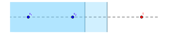
Figure 7: The intersection of the two halfspaces is $V_{T}({s_{1},s_{2}})$.

We hence conclude that a halfspace can be constructed using $|S|=2$ and $|T|=3$. Observe that it is also possible to do the same construction for $|S|\in\{2,3\}$ and $|T|=4$. We prove this explicitly in the next statement.

Proposition 3.6.

Let $F\subset\mathbb{R}^{n}$ be a halfspace. Then for any two integers $\tau>\sigma\geq 1$ there exist $S\subset T\subset\mathbb{R}^{n}$, with $|S|=\sigma$ and $|T|=\tau$, such that $V_{T}(S)=F$.

Proof.

Note that any halfspace $F$ can be represented as $F=\{x\in\mathbb{R}^{n}\,|\,\langle d,x\rangle\leq\gamma\}$ for some $d$, $\|d\|=1,$ and $\gamma\in\mathbb{R}$. Choose any $x_{0}$ such that $\langle d,x_{0}\rangle=\gamma$, and let $S:=\{s_{0},\dots,s_{m}\}$ and $T:=\{t_{0},\dots,t_{p}\}\cup S$, where $m=\sigma-1$, $p=\tau-\sigma-1$,

$$s_{0}:=x_{0}-d,\text{ }t_{0}:=x_{0}+d,$$

$$s_{i}=x_{0}-\alpha_{i}d,\;0<\alpha_{i}<1\;\forall i\in\{1,\dots,m\},\;t_{j}:=x_{0}+\beta_{j}d,\,\beta_{j}>1\;\forall j\in\{1,\dots,p\},$$ (25)

and the constants $\alpha_{i}$ and $\beta_{j}$ are all different (to ensure that the sites do not coincide). We will next show that

$$V_{T}(S)=\{x\in\mathbb{R}^{2}\,|\,\langle d,x\rangle\leq\gamma\}.$$

We have, from the representation in Proposition 2.1,

$$V_{T}(S)=\bigcap_{\begin{subarray}{c}i\in\{0,1,\dots,m\}\\ j\in\{0,1,\dots,p\}\end{subarray}}\left\{x\,:\,\langle t_{j}-s_{i},x\rangle\leq\frac{1}{2}\left(\|t_{j}\|^{2}-\|s_{i}\|^{2}\right)\right\}.$$

By (25), the inequalities in the latter expression can be rewritten as

$$(\beta_{j}+\alpha_{i})\langle d,x\rangle\leq\frac{1}{2}\left((\beta_{j}-\alpha_{i})(\beta_{j}+\alpha_{i})+(\beta_{j}+\alpha_{i})\langle d,x_{0}\rangle\right),\;\begin{array}[]{l}\forall i\in\{0,\dots,m\},\\ \forall j\in\{0,\dots,p\},\end{array}$$

where $\alpha_{0}=\beta_{0}=1$. Dividing by the factor $\beta_{j}+\alpha_{i}>0$, we have

$$\langle d,x\rangle-\langle d,x_{0}\rangle\leq\frac{\beta_{j}-\alpha_{i}}{2};$$

hence,

$$V_{T}(S)=\left\{x\,:\,\langle d,x\rangle-\gamma\leq\frac{1}{2}\cdot\min_{i,j}(\beta_{j}-\alpha_{i})\right\}=\{x\,:\,\langle d,x\rangle\leq\gamma\}.$$

The latter set is precisely the halfspace that we were aiming for. ∎

3.6 Intersections of Parallel Halfspaces

We consider a set $F\subset\mathbb{R}^{n}$ represented by the inequalities $\alpha\leq\left\langle d,x\right\rangle\leq\beta,$ with $\left\|d\right\|=1$ and $\alpha<\beta.$ One can easily check that $F=V_{T}\left(S\right)$ for $T:=\left\{s_{1},s_{2},t_{1},t_{2}\right\}$ and $S:=\left\{s_{1},s_{2}\right\}$ with, for instance, $s_{1}:=\frac{3\alpha+\beta}{4}d,$ $s_{2}:=\frac{\alpha+\beta}{2}d,$ $t_{1}:=\frac{3\alpha-\beta}{2}d$ and $t_{2}:=\frac{7\beta-3\alpha}{4}d.$ We have shown the following result.

Proposition 3.7.

Let $F\subset\mathbb{R}^{n}$ be an intersection of two parallel halfspaces with opposite normals, such that $F$ has a nonempty interior. Then there exist $S\subset T\subset\mathbb{R}^{n}$, with $|S|=2$ and $|T|=4$, such that $V_{T}(S)=F$.

Note that it is impossible to produce a strip with $|T|-|S|=1$: indeed, it is clear from the fact that all constraints are defined by parallel lines that all vectors $s-t$, $s\in S$, $t\in T$ should be colinear, lying on some line orthogonal to the inequalities. Now, if for the unique $t\in T\setminus S$ we have $t\in\operatorname{conv}S$, then the cell is empty by Corollary 2.2. However if $t\notin\operatorname{conv}S$, then the cell has to be a halfspace. Hence the only possibility is $|T|=4$, $|S|=2$.

3.7 Wedges

Now, let us have a wedge $F:=\left\{x\in\mathbb{R}^{n}:\left\langle c_{i},x\right\rangle\leq\alpha_{i},\text{ }i=1,2\right\},$ with $c_{1}$ and $c_{2}$ being linearly independent. Let us take an arbitrary point from $t\in\operatorname{int}F^{-}:=\left\{x\in\mathbb{R}^{n}:\left\langle c_{i},x\right\rangle\geq\alpha_{i},\text{ }i=1,2\right\}$ and construct the two symmetric points $s_{1}$ and $s_{2}$ with respect to both hyperplanes defining $F.$ If $T:=\left\{s_{1},s_{2},t\right\}$ and $S:=\left\{s_{1},s_{2}\right\},$ then $V_{T}\left(S\right)=F_{T}(t)=F.$

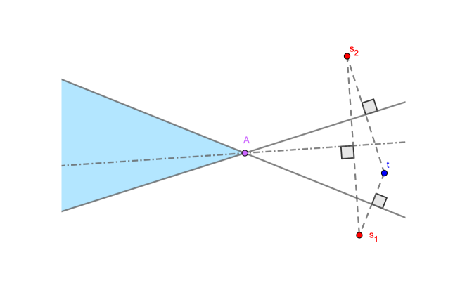
Figure 8: Construction of the set of sites for a wedge

It is possible to add any number of more sites $s$ to $S$ in such a way that the halfspaces $\|s-x\|\leq\|t-x\|$ include the original wedge.

Proposition 3.8.

Let

$$F:=\left\{x\in\mathbb{R}^{n}\,|\,\langle v_{i},x\rangle\leq b_{i},\quad i=1,2\right\},$$

with $v_{1,}v_{2}\in\mathbb{R}^{n}$ linearly independent unit vectors and $b_{1},b_{2}\in\mathbb{R}.$ Then there exist $S\subset T\subset\mathbb{R}^{n},$ with $|S|=2$ and $|T|=4,$ such that $V_{T}(S)=F$.

Proof.

Without loss of generality, we assume that $b_{i}=0$ $\left(i=1,2\right).$ Set $\beta:=\left\langle v_{1},v_{2}\right\rangle,$ $i^{\prime}:=3-i$ for $i=1,2,$ and define

$$s_{i}:=-v_{i}-2v_{i^{\prime}}\text{\qquad}\left(i=1,2\right).$$

Let $t_{i}$ be the point symmetric to $s_{i}$ with respect to the hyperplane defined by $\langle x,v_{i^{\prime}}\rangle=0,$ that is,

$$t_{i}:=-v_{i}+2\left(1+\beta\right)v_{i^{\prime}}\text{\qquad}\left(i=1,2\right),$$

and define $S:=\left\{s_{1},s_{2}\right\}$ and $T:=\left\{s_{1},s_{2},t_{1,}t_{2}\right\}.$ We have $|T|=4,$ since $\beta>-1.$ Given that

$$\left\|t_{i}\right\|^{2}=5+4\beta=\|s_{i}\|^{2}\text{\qquad}\left(i=1,2\right),$$

one has

$$V_{T}(S)=\left\{x\in\mathbb{R}^{n}\,|\,\langle t_{i}-s_{i},x\rangle\leq 0,\;\langle t_{i}-s_{i^{\prime}},x\rangle\leq 0,\text{\qquad}i=1,2\right\}.$$ (26)

Hence, to prove that $V_{T}(S)=F,$ it will suffice to show that, for $i=1,2,$ the inequality $\langle x,t_{i}-s_{i}\rangle\leq 0$ is equivalent to $\langle x,v_{i^{\prime}}\rangle\leq 0$ and that the remaining two inequalities in (26) are redundant. The first assertion is obvious, since $t_{i}-s_{i}=2\left(2+\beta\right)v_{i^{\prime}}$ and $\beta>-1.$ Let us now prove that the inequalities $\langle t_{i}-s_{i^{\prime}},x\rangle\leq 0$ are redundant, that is, that they are consequences of the system $\langle v_{i},x\rangle\leq 0$ $\left(i=1,2\right).$ But this is also immediate, since $t_{i}-s_{i^{\prime}}=v_{i}+\left(3+2\beta\right)v_{i^{\prime}}$ and $\beta>-1.$ ∎

3.8 Unbounded Polygons with Three Sides

Our next construction is for an unbounded polygon like the shadowed one in Fig. 9,

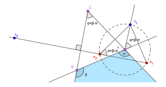
Figure 9: Unbounded polygon with three sides

with three sides, which is unbouned and has non-parallel sides.

Proposition 3.9.

Let $F$ be an unbounded convex polygon with non-parallel sides and two vertices. Then there exist $S\subset T\subset\mathbb{R}^{2}$, with $|S|=2$ and $|T|=4$, such that $V_{T}(S)=F$.

Proof.

In the notation of Fig. 9, where $F$ is depicted as the shaded region, we would like to mention that $0<\alpha<\pi$, $0<\beta<\pi$, $\alpha+\beta>\pi$ and $\beta\geq\alpha$. If we consider the triangle $ABC,$ the angle at $C$ is $\alpha+\beta-\pi.$ Now, we draw a line through the point $A,$ which makes an angle $\alpha+\beta-\pi$ with the line $BA.$ On this line we consider an arbitrary point $t_{1}$, sufficiently close to $A.$ Let us take the symmetric points $s_{1}$ and $s_{2}$ of $t_{1}$ with respect to $AB$ and $AC,$ respectively. We shall prove that the line through the points $s_{1}$, $s_{2}$ is perpendicular to $BC.$ For this purpose, we would like to mention that the point $A$ is the center of the circle passing through the points $s_{1}$, $s_{2}$ and $t_{1}.$ This means that $\sphericalangle s_{1}s_{2}t_{1}=\alpha+\beta-\pi.$ If we consider the quadrilateral formed by the lines $BC,$ $AC,$ $s_{1}s_{2}$ and $t_{1}s_{2},$ we get the desired fact. At the end we construct the site $t_{2}$ as the symmetric point of $s_{1}$ with respect to the line $BC\$and set $S:=\left\{s_{1},s_{2}\right\}$ and $T:=\left\{s_{1},s_{2},t_{1},t_{2}\right\}$. ∎

Proposition 3.10.

Let $S\subset T\subset\mathbb{R}^{2},$ with $|S|=2$ and $|T|=4.$ Then $V_{T}(S)$ is not an unbounded polygon with parallel sides and just two vertices.

Proof.

Similarly to the proof of Proposition 3.3, suppose that $V_{T}\left(S\right)$ is an unbounded convex polygon with parallel sides and just two vertices, denote $S=\{s_{1},s_{2}\}$ and $T=\{s_{1},s_{2},t_{1},t_{2}\},$ and suppose further, w.l.o.g., that the redundant inequality in the linear system

$$\left\langle t_{i}-s_{j},x\right\rangle\leq\frac{1}{2}\left(\left\|t_{i}\right\|^{2}-\left\|s_{j}\right\|^{2}\right)\text{\quad}\left(i,j=1,2\right)$$ (27)

(which has $V_{T}(S)$ as its solution set) is the one corresponding to $i=2=j.$ Then, by Farkas’ Lemma, there exist $\gamma_{11},\gamma_{12},\gamma_{21}\geq 0$ such that

$$t_{2}-s_{2}=\gamma_{11}\left(t_{1}-s_{1}\right)+\gamma_{12}\left(t_{1}-s_{2}\right)+\gamma_{21}\left(t_{2}-s_{1}\right)$$ (28)

and

$$\alpha_{22}\geq\gamma_{11}\alpha_{11}+\gamma_{12}\alpha_{12}+\gamma_{21}\alpha_{21},$$ (29)

where $\alpha_{ij}:=\frac{1}{2}\left(\left\|t_{i}\right\|^{2}-\left\|s_{j}\right\|^{2}\right).$ From (28) we obtain that $t_{2}-s_{2}$ belongs to

$$K_{1}:=\operatorname{cone}\left\{t_{1}-s_{1},t_{1}-s_{2},t_{2}-s_{1}\right\}.$$

On the other hand, two of the three vectors $t_{1}-s_{1},$ $t_{1}-s_{2}$ and $t_{2}-s_{1}$ are exterior normals to the parallel sides, and hence they make an angle of $\pi.$ Those two vectors cannot be $t_{1}-s_{1}$ and $t_{1}-s_{2},$ because with such a configuration $V_{T}(S)$ would be empty. We will consider the two remaining cases. We start with the case when the two vectors are $t_{1}-s_{1}$ and $t_{2}-s_{1},$ say $t_{1}-s_{1}=-\mu\left(t_{2}-s_{1}\right),$ with $\mu>0.$ Since in this case $s_{2}$ does not belong to the straight line determined by $s_{1},$ $t_{1}$ and $t_{2}$ (because the side of $V_{T}(S)$ contained in the line $\left\langle t_{1}-s_{2},x\right\rangle=\frac{1}{2}\left(\left\|t_{1}\right\|^{2}-\left\|s_{2}\right\|^{2}\right)$ is not parallel to the other two sides), there is a circle containing $s_{2},$ $t_{1}$ and $t_{2},$ and we may assume, w.l.o.g., that the center of this circle is $0_{2}.$ Then $\alpha_{11}=\alpha_{21}>0$ and $\alpha_{12}=\alpha_{22}=0,$ thus, in view of (29), we have $\gamma_{11}=0=\gamma_{12}$ and then, by (28),

$$\gamma_{12}\left(t_{1}-s_{2}\right)=t_{2}-s_{2}=-\left(t_{1}-s_{1}\right)+t_{1}-s_{2}+t_{2}-s_{1}=t_{1}-s_{2}+\left(1+\mu\right)\left(t_{2}-s_{1}\right),$$

which yields

$$t_{2}-s_{1}=\frac{\gamma_{12}-1}{1+\mu}\left(t_{1}-s_{2}\right).$$

This is impossible because the vectors $t_{1}-s_{1},$ $t_{1}-s_{2}$ and $t_{2}-s_{1}$ are not all colinear. It only remains to consider the case when $t_{1}-s_{2}$ and $t_{2}-s_{1}$ are the vectors that make an angle of $\pi.$ Since $t_{1}-s_{1}$ is not colinear with these two vectors, we have that the cones $K_{1}$ and

$$K_{2}:=\operatorname{cone}\left\{-\left(t_{1}-s_{1}\right),t_{1}-s_{2},t_{2}-s_{1}\right\}$$

are opposite halfplanes defined by the line containing the vectors $t_{1}-s_{2}$ and $t_{2}-s_{1}.$ The fact that $t_{2}-s_{2}\in K_{1}\cap\operatorname{int}K_{2}$ provides a contradiction. ∎

We note here that it is possible to have an unbounded polygon with three sides for the case $|S|=3$ and $|T|=4$ if and only if the unbounded sides are non-parallel. Indeed, in this case we can first build a wedge that defines the two unbounded sides (see Subsection 3.7), and then add an extra site to define the extra inequality. For the case of unbounded parallel sides, it is clear that the point $t$ should at the same time lie outside of each of these parallel sides, which is impossible.

3.9 Unbounded Polygons with Four Sides

In the next proposition we shall consider the case of an unbounded quadrilateral in $\mathbb{R}^{2}$ with two parallel sides, shown in Fig. 10.

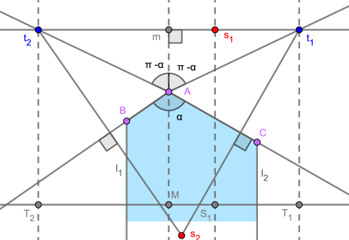
Figure 10: Unbounded polygon with parallel sides

Proposition 3.11.

Let $F\subset\mathbb{R}^{2}$ be an unbounded convex quadrilateral with two parallel sides. Then there exist $S\subset T\subset\mathbb{R}^{2}$, with $|S|=2$ and $|T|=4$, such that $V_{T}(S)=F$.

Proof.

In the notation of Fig. 10, where $F$ is depicted as the unboubed convex polygon with vertices $A,$ $B$ and $C,$ we have $l_{1}\parallel l_{2}$ and $0<\alpha<\pi,$ and the point $A$ belongs to the interior of the parallel band. First, we move, parallel to the line $l_{1},$ the point $A$ to an arbitrary point $M$. Through $M$ we draw a line perpendicular to $l_{1}.$ Take a point $S_{1}$ on the same line, with the same distance to $l_{2}$ as $M$ is to $l_{1}.$ Now, we consider the symmetrical point $T_{1}$ and $T_{2}$ of $S_{1}$ with respect to $l_{2}$ and $l_{1},$ respectively. In this way $M$ is the midpoint of the segment $T_{1}T_{2}$. Next we translate the line through the points $T_{1}$ and $T_{2}$ in such a way that, defining $t_{1},$ $t_{2},$ $m$ and $s_{1}$ as the orthogonal projections of $T_{1},$ $T_{2},$ $M$ and $S_{1}$ onto the resulting translated line, one has $\sphericalangle$ $t_{1}At_{2}=2\pi-2\alpha$ and $\sphericalangle$ $mAt_{2}=\pi-\alpha.$ For the last site, we take $s_{2}$ as the symmetric point of $t_{2}$ with respect to the line through the points $A$ and $B.$ We shall prove that the line through the points $t_{1}$, $s_{2}$ is perpendicular to $AC.$ For this purpose, we observe that the point $A$ is the center of the circle passing through the points $t_{1}$, $t_{2}$ and $s_{2}.$ This means that $\sphericalangle t_{2}s_{2}t_{1}=\pi-\alpha.$ If we consider the quadrilateral formed by the lines $BA,$ $AC,$ $t_{1}s_{2}$ and $t_{2}s_{2},$ we get the desired fact. At the end, after having found the desired sets $S:=\left\{s_{1},s_{2}\right\}$ and $T:=\left\{s_{1},s_{2},t_{1},t_{2}\right\}$, we would like to mention that this construction is impossible if $\alpha=\pi.$ ∎

We next consider the case of an arbitrary unbounded convex quadrilateral with nonparallel sides, presented in Fig. 11.

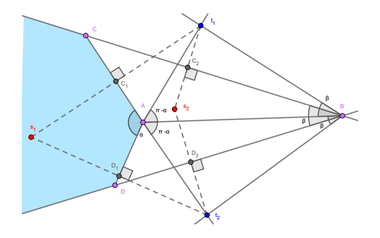
Figure 11: Configuration for a general unbounded quadrilateral

Proposition 3.12.

Let $F$ be an unbounded convex quadrilateral with no sides parallel. Then there exist $S\subset T\subset\mathbb{R}^{2}$, with $|S|=2$ and $|T|=4$, such that $V_{T}(S)=F$.

Proof.

First, looking at Fig. 11, where $F$ is depicted as the shaded region, we obtain the point $B$ as the intersection of the unbounded sides of the convex quadrilateral with vertices $CAD$. We denote $\sphericalangle CAD=\alpha$ and $\sphericalangle CBD=\beta$ and observe that $\pi>\alpha>\beta>0.$ We next draw the lines that make angles $\pi-\alpha$ with $AB$ at the point $A$ and those that make angles $\beta$ with the same segment at $B.$ We then get the points $t_{1}$ and $t_{2}$ as the two other vertices of the quadrilateral determined by these four lines. We take $s_{1}$ and $s_{2}$ as the symmetric points of $t_{1}$ with respect to $CA$ and $CB,$ respectively. To see that $V_{T}(S)=F$ for $S:=\left\{s_{1},s_{2}\right\}$ and $T:=\left\{s_{1},s_{2},t_{1},t_{2}\right\},$ the only thing that we have to prove is that $t_{2}s_{1}\bot AD$ and $t_{2}s_{2}\bot BD.$ The pòint $B$ is the center of the circle passing through the points $t_{1},$ $t_{2}\$and$\ s_{2}.$ Therefore, $\sphericalangle t_{1}s_{2}t_{2}=\pi-\beta,$ which, looking at the quadrilateral $C_{2}s_{2}D_{2}B,$ implies that $t_{2}s_{2}\bot BD.$ The point $A$ is the center of the circle passing through the points $t_{1},$ $t_{2}$ and$\ s_{1}.$ Therefore, $\sphericalangle t_{1}s_{1}t_{2}=\pi-\alpha,$ which, looking at the quadrilateral $C_{1}s_{1}D_{1}A,$ implies $t_{2}s_{1}\bot AD.$ ∎

4 Conclusions

We have obtained constructive characterizations of properties pertaining to higher-order Voronoi cells, and applied these characterizations to a case study of cells of order at least two in the system of four sites.

In particular, the results obtained in the preceding subsections show that for $S\subset T\subset\mathbb{R}^{2}$, with $|S|=2$ and $|T|=4$, the resulting cell $V_{T}(S)$ can be any of the following sets: the empty set, a singleton, a non-cyclic bounded convex quadrilateral, a halfplane, an intersection of parallel halfplanes with opposite normals and a nonempty interior, an angle, an unbounded polygon with non-parallel sides and just two vertices, or an unbounded convex quadrilateral. All the remaining possibilities for sets in $\mathbb{R}^{2}$ de ned by four linear inequalities, namely, a singleton, a one-dimensional set, a triangle, a cyclic quadrilateral, and an unbounded quadrilateral with parallel sides and just two vertices are unfeasible.

The restrictions on the possible shapes of higher-order cells discovered in our case study are consistent with the challenges encountered in the design of numerical methods for constructing higher-order cells (cf. [14]), where the key assumption of general position ensures the absence of cyclic quadrilateral configurations). Thus a natural direction for the future study is to obtain general structural results on the shapes of higher-order cells, which will in turn inform the design of algorithms. For instance, we would like to know whether the convex hull of affinely independent points can be represented as a higher-order Voronoi cell (generalizing our result on the impossibility of a triangular cell), what higher-dimensional configurations produce cells with empty interiors, and what are the possible dimensions of higher-order Voronoi cells in $\mathbb{R}^{n}$.

5 Acknowledgments

We are grateful to the two JOTA referees for their thoughtful and thorough corrections and suggestions, including the proof of Proposition 3.10. These corrections have greatly improved the quality of our paper.

The first author was supported by the MINECO of Spain, Grant MTM2014-59179-C2-2-P, and the Severo Ochoa Programme for Centres of Excellence in R&D [SEV-2015-0563]. He is affiliated to MOVE (Markets, Organizations and Votes in Economics). He thanks The School of Mathematics and Statistics of UNSW Sydney for sponsoring a visit to Sidney to complete this work.

The second author is grateful to the Australian Research Council for continuous financial support via grants DE150100240 and DP180100602, which in particular sponsored a trip to Barcelona that initiated this collaboration.

The third author was partially supported by MINECO of Spain and ERDF of EU, Grant MTM2014-59179-C2-1-P, and Sistema Nacional de Investigadores, Mexico.

References

- [1] Shamos, M., Hoey, D.: Closest-point problems. 16th Annual Symposium on Foundations of Computer Science (sfcs 1975) pp. 730–743 (1975)
- [2] Papadopoulou, E., Zavershynskyi, M.: On higher order Voronoi diagrams of line segments. In: Algorithms and computation, Lecture Notes in Comput. Sci., vol. 7676, pp. 177–186. Springer, Heidelberg (2012)
- [3] Goberna, M.A., Martínez-Legaz, J.E., Vera de Serio, V.N.: The Voronoi inverse mapping. Linear Algebra Appl. 504, 248–271 (2016)
- [4] Mallozzi, L., Puerto, J.: The geometry of optimal partitions in location problems. Optim. Lett. 12(1), 203–220 (2018)
- [5] Gemsa, A., Lee, D.T., Liu, C.H., Wagner, D.: Higher order city Voronoi diagrams. In: Algorithm theory—SWAT 2012, Lecture Notes in Comput. Sci., vol. 7357, pp. 59–70. Springer, Heidelberg (2012)
- [6] Kaplan, H., Mulzer, W., Roditty, L., Seiferth, P., Sharir, M.: Dynamic planar Voronoi diagrams for general distance functions and their algorithmic applications. In: Proceedings of the Twenty-Eighth Annual ACM-SIAM Symposium on Discrete Algorithms, pp. 2495–2504. SIAM, Philadelphia, PA (2017)
- [7] Klein, R.: Abstract Voronoĭ diagrams and their applications (extended abstract). In: Computational geometry and its applications (Würzburg, 1988), Lecture Notes in Comput. Sci., vol. 333, pp. 148–157. Springer, New York (1988)
- [8] O’Neil, P., Wanner, T.: Analyzing the squared distance-to-measure gradient flow system with k-order voronoi diagrams. Discrete & Computational Geometry (2018)
- [9] Qiu, C., Shen, H., Chen, K.: An energy-efficient and distributed cooperation mechanism for-coverage hole detection and healing in wsns. IEEE Transactions on Mobile Computing 17(6), 1247–1259 (2018)
- [10] Giansiracusa, N., Ricciardi, C.: Spatial analysis of U.S. Supreme Court 5-to-4 decisions (2018)
- [11] Kolahdouzan, M., Shahabi, C.: Voronoi-based k nearest neighbor search for spatial network databases. In: Proceedings of the Thirtieth International Conference on Very Large Data Bases - Volume 30, VLDB ’04, pp. 840–851. VLDB Endowment (2004)
- [12] Goberna, M.A., López, M.A.: Linear semi-infinite optimization, Wiley Series in Mathematical Methods in Practice, vol. 2. John Wiley & Sons, Ltd., Chichester (1998)
- [13] Goberna, M.A., Lopez, M.A., Todorov, M.: Stability theory for linear inequality systems. SIAM J. Matrix Anal. Appl. 17(4), 730–743 (1996)
- [14] Zavershynskyi, M., Papadopoulou, E.: A sweepline algorithm for higher order Voronoi diagrams. In: 2013 10th International Symposium on Voronoi Diagrams in Science and Engineering, pp. 16–22 (2013). DOI 10.1109/ISVD.2013.17