High-mass star formation at sub-50 AU scales .

Abstract

Context. The hierarchical process of star formation has so far mostly been studied on scales from thousands of au to parsecs, but the smaller sub-1000 au scales of high-mass star formation are still largely unexplored in the submm regime.

Aims. We aim to resolve the dust and gas emission at the highest spatial resolution to study the physical properties of the densest structures during high-mass star formation.

Methods. We observed the high-mass hot core region G351.77-0.54 with the Atacama Large Millimeter Array with baselines extending out to more than 16 km. This allowed us to dissect the region at sub-50 au spatial scales.

Results. At a spatial resolution of 18/40 au (depending on the distance), we identify twelve sub-structures within the inner few thousand au of the region. The brightness temperatures are high, reaching values greater 1000 K, signposting high optical depth toward the peak positions. Core separations vary between sub-100 au to several 100 and 1000 au. The core separations and approximate masses are largely consistent with thermal Jeans fragmentation of a dense gas core. Due to the high continuum optical depth, most spectral lines are seen in absorption. However, a few exceptional emission lines are found that most likely stem from transitions with excitation conditions above 1000 K. Toward the main continuum source, these emission lines exhibit a velocity gradient across scales of 100-200 au aligned with the molecular outflow and perpendicular to the previously inferred disk orientation. While we cannot exclude that these observational features stem from an inner hot accretion disk, the alignment with the outflow rather suggests that it stems from the inner jet and outflow region. The highest-velocity features are found toward the peak position, and no Hubble-like velocity structure can be identified. Therefore, these data are consistent with steady-state turbulent entrainment of the hot molecular gas via Kelvin-Helmholtz instabilities at the interface between the jet and the outflow.

Conclusions. Resolving this high-mass star-forming region at sub-50 au scales indicates that the hierarchical fragmentation process in the framework of thermal Jeans fragmentation can continue down to the smallest accessible spatial scales. Velocity gradients on these small scales have to be treated cautiously and do not necessarily stem from disks, but may be better explained with outflow emission. Studying these small scales is very powerful, but covering all spatial scales and deriving a global picture from large to small scales are the next steps to investigate.

1 Introduction

Star formation is an intrinsically hierarchical process where fragmentation occurs on almost all scales, from the large-scale molecular clouds with sizes of several ten to hundred pc, down to close binary formation at the center of dense cores and disk fragmentation that can lead to planets. In that framework, the smallest scale fragmentation of the cores and potentially also the disks are poorly understood, in particular for regions forming high-mass stars ($>8$ M_⊙) because they are typically located at distances of several kpc. Until recently, the state-of-the-art observations had as high resolution as $\sim$0.2^′′, allowing for the investigation of the fragmentation processes of the larger-scale molecular gas clumps into their cluster-forming cores (e.g., Beuther et al. 2007; Bontemps et al. 2010; Palau et al. 2013, 2014; Beuther et al. 2013; Csengeri et al. 2017; Cesaroni et al. 2017; Beuther et al. 2018). To understand the formation of close binaries or systems like the Trapezium in Orion (e.g., Preibisch et al. 1999), higher spatial resolution is needed. Furthermore, many other physical processes take place on small spatial scales. For example, disk-like structures as well as the inner jet and outflow regions are found on scales on the order of 10 to a few 100 au (e.g., Tan et al. 2014; Frank et al. 2014; Beltrán & de Wit 2016), again requiring the highest spatial resolution possible. Additionally important are global infall and streamer-like motions through which the material can get channeled in the innermost regions (e.g., Maud et al. 2017; Goddi et al. 2018).

Figure 1: Spectra of the four spectral windows extracted toward the main mm continuum peak position mm1. Clearly most lines are seen in absorption against the continuum, only a few in emission. Selected spectral lines are labeled.

Millimeter and centimeter wavelengths are the ideal spectral regime to study these processes because the young disks and jets are still deeply embedded within their natal cores. Sub-$0.1^{\prime\prime}$ spatial resolution can be achieved with the Very Large Array at cm wavelengths (e.g., Moscadelli & Goddi 2014; Beuther et al. 2017a), and now also with the Atacama Large Millimeter Array (ALMA) at (sub)mm wavelengths (e.g., Partnership et al. 2015).

Our target region is the well-known high-mass star-forming region G351.77-0.54 (a.k.a. IRAS 17233-3606). The distance to the target is debated, and while early studies put it at 2.2 kpc (Norris et al., 1993), more recent investigations favor smaller distances around 1 kpc (Leurini et al., 2011a). Since the accurate distance is not clear yet, in the following, we will always give the parameters for both distances. The luminosity and mass of the entire region are estimated to be $1.7\times 10^{4}/10^{5}$ L_⊙ and 660/3170 M_⊙ at 1/2.2 kpc, respectively (Norris et al., 1993; Leurini et al., 2011a, b). These numbers clearly show that we are dealing with a massive star-forming region on its way to form high-mass stars. The region exhibits linear CH₃OH class II maser features as well as strong outflow emission (e.g., Norris et al. 1993; Walsh et al. 1998; Leurini et al. 2009, 2013; Klaassen et al. 2015). Furthermore, this region is a very bright (sub)mm line emission source. Centimeter-wavelength interferometric studies revealed strong NH₃(4,4)/(5,5) emission at temperatures above 200 K and resolving overall rotational motion on a few 1000 au scales (Beuther et al., 2009), approximately perpendicular to the larger-scale outflow. Following Leurini et al. (2011a), we use as $\varv_{\rm lsr}$ a value of $\sim-3.6$ km s^-1. Since Zapata et al. (2008) found six cm continuum sources within that core, it was expected that this region would show fragmentation on smaller spatial scales in the (sub)mm regime. Furthermore, multiple outflows have been identified (e.g., Leurini et al. 2009, 2011a; Klaassen et al. 2015; Beuther et al. 2017b). In a recent ALMA study of this region at 690 GHz we resolved the region at 0.06^′′ resolution (Beuther et al., 2017b). This study revealed at least four sub-cores where the central source #1 provide strong evidence for rotational motion on scales of a few hundred au, perpendicular to an outflow seen in CO(6–5). But ALMA can go to even higher spatial resolution, and here we present a study of the same region at $\sim$1.3 mm wavelengths and 21 mas$\times$15 mas resolution, corresponding to $\sim$18/40 au at a distance of 1/2.2 kpc.

2 Observations

The target high-mass star-forming region G351.77-0.54 was observed with ALMA as a cycle 3 project (id 2015.1.00496) in four separate observing blocks between Nov. 5 and Dec. 2, 2015. The duration of the four scheduling blocks varied between 1 and 1.6 hours with on-source target observing times between 24 and 45 minutes. Between 33 and 43 antennas were in the array and baselines between 17 m and more than 16 km were covered. The phase center of our observations was R.A. (J2000.0) 17:26:42.568 and Dec. (J2000.0) -36:09:17.60. To calibrate the phases on the long baselines, short cycle times were used between the target and the phase and amplitude calibrator J1733-3722 with a typical cycle times consisting of $\sim$55 sec on source and $\sim$18 sec on the calibration quasar. Bandpass and flux calibration were conducted with the sources J1517-2422 and J1617-5848, respectively. The precipitable water vapor (PWV) varied between 0.42 and 0.93 mm. The 1.3 mm band 6 receivers were tuned to the LO frequency of 226.378 GHz with two spectral windows (spws) in the upper and lower sidebands, respectively. The frequency coverages of the four spectral windows is depicted in Fig. 1. The spectral resolution of the spws was 244 kHz, 488 kHz, and for the wider spectral windows 3906 kHz, corresponding to velocity resolutions of $\sim$0.33, $\sim$0.67 and 5.3 km s^-1, respectively. The primary beam of ALMA at these frequencies is $\sim$27^′′.

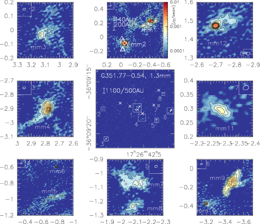
Figure 2: ALMA 1.3 mm continuum data toward the high-mass star-forming region G351.77-0.54 at an angular resolution of $0.021^{\prime\prime}\times 0.015^{\prime\prime}$. The central panel shows the overall structure (the white crosses mark the cm continuum source positions from Zapata et al. 2008), and the surrounding panels show selected zooms into the areas marked in the central panel. We note the different cutout sizes of the individual zoom windows. The contour levels always start at a $4\sigma$ level of 0.2 mJy beam^-1 and continue in $4\sigma$ steps. Scale bars assuming 1.0/2.2 kpc distance are shown in the middle and middle-top panels. The middle-top panel also shows the CH₃OH maser positions from Walsh et al. (1998) and an intensity scale. The synthesized beam is presented in each panel.

The calibration of the data was done with the ALMA pipeline in CASA (McMullin et al., 2007) version 4.5.0 following the scripts provided by the observatory. In a following step, we applied phase-only self-calibration to the data going down to time-steps of 30 sec. Images prior and after self-calibration were carefully compared, and while all structures are well recovered, the noise is decreased after self-calibration. No amplitude self-calibration was applied.

The following imaging was also conducted within CASA. Although some baselines between 17 and 55 m are observed, their coverage is sparsely sampled, and so do not allow us to reasonably image the larger-scale emission. Therefore, in the imaging process we only used data from baselines longer than 55 m, which allows us to concentrate on the most compact structures. As visible in Fig. 1, this hot core hosts many spectral lines and defining line-free parts of the spectrum is not easy. Therefore, we compared different approaches to create a continuum image of the region. On the one hand, we produced a continuum image from only a small part of the spectrum that appears line-free, and on the other hand, we produced a continuum image from the whole bandpass with all spectral features included. Structurally and with respect to the intensities, there was barely any difference between the two images, only the noise of the full-bandpass image was lower. Therefore, in the following we use the continuum image created from the whole bandpass. For the continuum images we applied a robust weighting of -2, corresponding to uniform weighting. This results in a synthesized beam of 21 mas $\times$ 15 mas with a position angle of -74^∘. A few apparently line-free parts of the spectra were used for the continuum subtraction. However, in such a line-rich source, this is not a trivial process and some weak bandpass slope remains (Fig. 1). However, that slope is so weak that is does not affect any of the analyses. The line data were then imaged with a robust weighting of 0, resulting in a slightly larger synthesized beam of $\sim$25 mas $\times$ 20 mas with a position angle of -86^∘. The continuum 1$\sigma$ rms is $\sim$50 $\mu$Jy beam^-1, and the typical rms for the spectral lines in a line-free channel of 1 km s^-1 width is $\sim$0.9 mJy beam^-1.

3 Results

As outlined in the previous Section 2 and shown in Fig. 1, extended emission is not well imaged in this long-baseline-only dataset, and most lines are mainly seen in absorption against the continuum sources. However, there are a few emission lines (Fig. 1) showing structure on small spatial scales below 100 au. Therefore, in the following we concentrate on the small-scale continuum emission as well as on the few transitions seen in emission.

3.1 Continuum emission and core fragmentation

Figure 2 presents a compilation of the 1.3 mm continuum data of the region. While the central panel shows the inner $\sim 7^{\prime\prime}\times 7^{\prime\prime}$, the surrounding 8 panels present zoom-ins for the sub-structure. With an angular resolution of $0.021^{\prime\prime}\times 0.015^{\prime\prime}$ (mean of $0.018^{\prime\prime}$), we can resolve linear structures of roughly 18/40 au at 1/2.2 kpc distance, among the highest spatial resolution observations achieved for high-mass star-forming regions today.

While at first sight, this image appears largely empty with only a few compact sub-structures distributed throughout, one should keep in mind that this image is strongly affected by missing flux because we only image data with baselines larger than 55 m (and extending to more than 16 km). Hence, all intermediate and large-scale structures are filtered out and we concentrate on the small sub-cores remaining. To get a feeling for the fraction of missing flux, we extract the 870 $\mu$m flux (central frequency 345 GHz) of G351.77-0.54 from the ATLASGAL survey (Schuller et al., 2009). Scaling the 870 $\mu$m peak flux density of 52.1 Jy beam^-1 (with a beam size of $19.2^{\prime\prime}$) with a flux dependency of $S\propto\nu^{4}$ to our central frequency of 226.6 GHz, approximately 9.7 Jy should be emitted in our field. However, as shown below, the sum of the fluxes of all identified sub-cores accumulates to only $\sim$208 mJy. Taking these numbers, we recover only about 2.1% of the total continuum emission in the field.

Table 1: Millimeter continuum emission parameters

name	R.A.	Dec.	$S_{\rm peak}$	$S_{\rm int}$	$T_{\rm b}$	mean $T_{\rm b}$	M@1.0kpca	M@2.2kpca	Nb
	(J2000.0)	(J2000.0)	(mJy/beam)	(mJy)	(K)	(K)	(M⊙)	(M⊙)	$(\times 10^{25}$cm-2)
mm1	17:26:42.533	-36:09:17.37	15.0	47.4	1144	53	0.41	2.0	3.3
mm2	17:26:42.563	-36:09:17.68	13.5	42.3	1027	93	0.20	1.0	3.0
mm3	17:26:42.827	-36:09:17.63	0.7	4.5	56	24	0.10	0.5	1.6
mm4	17:26:42.797	-36:09:20.50	1.9	21.0	152	44	0.22	1.1	4.5
mm5	17:26:42.506	-36:09:18.58	0.3	3.6	29	20	0.10	0.5	0.7
mm6	17:26:42.503	-36:09:18.19	1.4	1.4	111	50	0.01	0.1	3.2
mm7	17:26:42.395	-36:09:18.67	0.6	13.8	49	26	0.27	1.3	1.4
mm8	17:26:42.396	-36:09:18.83	0.6	3.0	52	24	0.06	0.3	1.4
mm9	17:26:42.280	-36:09:17.73	1.4	55.3	115	50	0.51	2.5	3.4
mm10	17:26:42.304	-36:09:17.97	1.3	3.7	101	32	0.06	0.3	2.9
mm11	17:26:42.379	-36:09:17.31	0.8	2.9	62	30	0.05	0.2	1.8
mm12	17:26:42.345	-36:09:16.13	4.0	10.5	310	38	0.13	0.6	9.4

Notes:
^a Masses are calculated using their mean brightness temperature $T_{\rm b}$.
^b Column densities are calculated using the peak brightness temperature $T_{\rm b}$.

Nevertheless, this spatial filtering also has strong advantages because we can isolate the compact structures within this region. With the sparse spatial sampling on short and intermediate baselines, and only a limited amount of emission features in the map, an automized source identification is not required. Therefore, we identify the source structures by eye following the 5$\sigma$ contours in Fig. 2. This way, we identify 12 separate mm sources within a radius of roughly $3.5^{\prime\prime}$ or 3500/7700 au at 1.0/2.2 kpc distance, respectively. Projected separations range from more than 1000 au to several 100 au. Some sources, for example, mm1 and mm2, show even smaller secondary peaks on scales below 100 au. The largest extended structures we can trace with these observations are found toward the sub-sources mm1, mm4 and mm8, and depending on the distance to the region, these sources have sizes between roughly 200 and 600 au. Taking mm9 as an example, and assuming the closer distance of 1 kpc, our spatial resolution corresponds to $\sim$18 au, and the extent of the source is roughly 300 au. This outlines the approximate spatial dynamic range covered by these data. None of the mm continuum sources are directly spatially associated with the cm continuum sources reported in Zapata et al. (2008) and marked in Fig. 2. In comparison to the 438 $\mu$m submm continuum sources presented in Beuther et al. (2017b), the here identified sources mm1 and mm2 correspond to their sources #1 and #2. The sources #3 and #4 in Beuther et al. (2017b) correspond to the mm sources mm12 and mm3, respectively. While the compact sources most likely host protostars, some of the more diffuse structures like mm5 or mm7 may not be of protostellar nature but could rather be remnants of the larger-scale envelope where only some imaged structure is left after the interferometric spatial filtering (see also Section 4.1).

At these spatial scales, optical depth effects can also become important, and one way to assess this is by converting the peak flux densities into peak brightness temperatures. Table 1 presents for all 11 identified sub-structures the peak flux densities $S_{\rm peak}$, the integrated fluxes $S_{\rm int}$ (integrated within the 4$\sigma$ contours), the corresponding peak brightness temperature $T_{\rm b}$ as well as the mean brightness temperatures derived again within the 4$\sigma$ contours of 16 K. As one sees, the peak brightness temperatures toward the strongest positions mm1 and mm2 exceed 1000 K, and toward the other peak positions are between 29 and 310 K. From the CH₃CN temperature analysis for this region at 690 GHz presented in Beuther et al. (2017b), we know that the gas temperatures around mm1 are also around 1000 K. This clearly shows that the dust emission in this region is optically thick and traces an inner core surface at the derived brightness temperature. Such high dust optical depth can also be inferred from the fact that almost all lines are seen in absorption against the mm1 continuum peak (Fig. 1). While the peak brightness temperatures in the other sub-structures are lower, they are still high compared to studies at slightly lower angular resolution (e.g., the NOEMA CORE survey at $\sim 0.4^{\prime\prime}$, Beuther et al. 2018).

What gas temperature would one expect for the outer sub-structures assuming the heating is dominated by the innermost core mm1? In this case we can do a simple estimate assuming a typical temperature distribution in dust and gas cores of $T\propto r^{-0.4}$ (e.g., van der Tak et al. 2000). Using 1000 K as the temperature at our resolution element (mean value $0.018^{\prime\prime}$), at the approximate spatial separation of the outer core structures of $3.5^{\prime\prime}$ one would get a temperature of $\sim$121 K. Taking into account that (a) the medium is not homogeneous, (b) there are probably several heating sources, and that (c) the 1000 K at the resolution element is an lower limit because it is an average over the beam size, the measured peak brightness temperatures do not deviate too much from the temperatures one could expect on these scales in such a region if they were heated by an internal source like mm1. It is likely that some of the lower intensity structures already have moderate optical depth at such high spatial resolution as well.

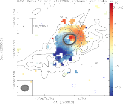
Figure 3: Color-scale shows for mm1 the first moment map (intensity-weighted peak velocities) from the line at 217.82 GHz. The contours are the 1.3 mm continuum data in $4\sigma$ level of 0.2 mJy beam^-1 up to a 3 mJy beam^-1 level (to avoid too many contours in the center). A scale-bar and the resolution elements of the line (gray) and continuum are shown as well. The arrow outlines the approximate direction of the CO(6–5) red outflow lobe shown in Fig. 6.

Although we argue that the dust emission has increased optical depth at several positions, we nevertheless would like to get rough estimates of the masses and column densities toward the individual sub-structures. Therefore, we use the typical approach to estimate masses from mm continuum emission assuming optically thin emission (e.g., Hildebrand 1983), but at the same time stress that the derived masses and column densities should be considered as lower limits. Following the equations outlined in Schuller et al. (2009) for dust emission, we are using for the 1.3 mm dust opacity $\kappa$ a value of 1.11 cm² g^-1 from Ossenkopf & Henning (1994) at high densities of $10^{8}$ cm^-3. Furthermore, a gas-to-dust mass ratio of 150 is assumed (Draine, 2011). Regarding the temperatures, since we are apparently dealing with optically thick emission, using the derived brightness temperature as an approximate proxy to estimate the actual temperatures seems a reasonable approach. For the column density estimates, we use 1000 K for the two very bright sources mm1 and mm2, and lower temperatures of 100 K for the other sources (depending on the dust optical depth peak brightness temperatures for some of the weaker sources may be lower limits for the actual gas temperature). Since the substructures are extended and cover a range of brightness temperatures, for the mass estimates, we derive for each core a mean brightness temperature within the $4\sigma$ contour (Table 1).

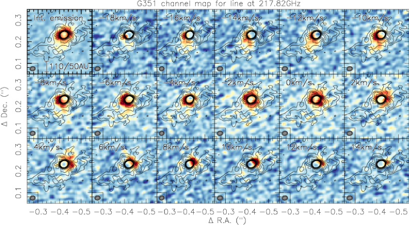
Figure 4: Channel map of the 217.82 GHz line for mm1. The top-left panel presents the integrated emission between -18 and +14 km s^-1. The remaining panels show the channels with 2 km s^-1 width at the velocities marked at the top-left of each panel. The contours are the 1.3 mm continuum data in $4\sigma$ level of 0.2 mJy beam^-1 up to a 3 mJy beam^-1 level (to avoid too many contours in the center). A scale-bar is shown in the top-left panel, and the resolution elements of the line (gray) and continuum are presented in each panel. The $\varv_{\rm lsr}$ is at approximately $-3.6$ km s^-1.

Table 1 presents the derived masses and column densities, and we stress that these values have to be considered as lower limits because of the high optical depth as well as the large amount of missing flux. Hence, although individual core masses between a fraction of a solar mass and 2 M_⊙ (depending on distance) do not seem very high, since they are lower limits and measured over very small size scales, they already indicate very high densities. For example, the almost spherical source mm2 has at 1 kpc distance a mass lower limit of 0.2 M_⊙ and a diameter of $\sim$100 au. Assuming that the three-dimensional structure of the core resembles a sphere, we can estimate a number density, and we derive high values for the approximate molecular hydrogen densities around $6.8\times 10^{10}$ cm^-3. The corresponding column densities are on the order of $10^{25}$ cm^-2, corresponding to visual extinction values around $10^{4}$ mag.

3.2 Emission lines and the dense inner entrained outflow/jet

As shown in the spectra in Fig. 1, we barely find any line emission signal in these data. On larger scales molecular emission is expected and also found in previous studies of this region (e.g., Leurini et al. 2011a; Beuther et al. 2009, 2017b), however, this emission is filtered out by these long baseline observations. In contrast to this, toward the compact mm peaks the brightness temperatures of the dust are so high that most lines are found only in absorption. However, there are a few lines seen in Fig. 1 that are indeed emission lines, even against the strong continuum with a peak brightness temperature above 1100 K. This implies that these spectral line emission features should stem from molecular lines with very high excitation levels E_u/K, most likely above 1000 K. Identifying these lines is tricky because one finds many possible line candidates in the typical databases (e.g., JPL Pickett et al. 1998, CDMS Müller et al. 2001, Splatalogue https://www.cv.nrao.edu/php/splat/). Table 2 presents the frequencies of the emission lines as well as possible transition candidates. Except for the SiO(5–4) line, we only list line candidates with excitation temperatures E_u/K above 500 K. We only list two to three possible candidates for each line, but going through the line catalogs, others are possible as well. Since we are mainly interested in the kinematics of the gas in this study, and not so much in the chemistry, the exact line identification is of lower importance here, and in the following, we refer to the lines only by their frequencies.

Table 2: Emission line parameters

frequency	possible lines	Eu/k
(GHz)		(K)
217.10	SiO(5–4) @ 217.10498	31.3
217.82	HDCO($26_{4,23}-25_{5,20}$) @217.82120	1218
	CH3CH2CN($65_{7,58}-65_{6,59}$) @217.82669	980
231.896	C2H3OCHO($96_{11,85}-95_{12,84}$) @231.89506	1439
	CH3CH2CN($57_{8,50}-58_{5,53}$) @231.90159	783
232.029	CH2CHCN($34_{7,28}-35_{6,29}$)v11=2 @232.02812	1063
	CH2CHCN($34_{7,27}-35_{6,30}$)v11=2 @232.03717	1063
232.693	H2O($5_{5,0}-6_{4,3}$) @232.68670a	3462
	CH2CHCN($28_{2,27}-28_{1,28}$)v15=1 @232.68736	683
	(CH3)2CO($43_{16,27}-43_{15,28}$)AA @232.69487	686
234.82	(CH3)2CO($67_{48,20}-67_{47,21}$)EE @234.81810	1912
	HC5N(88–87)v11=1 @234.81890	655
235.965	HCOOH($47_{6,42}-46_{7,39}$) @235.96447	1337
	CH2CHCN($63_{3,60}-64_{2,63}$)v11=1 @235.96961	1281

Notes: ^a suggested in Ginsburg et al. (2018)

All compact emission lines can be well imaged and they show mainly emission around mm1. Since the 217.82 GHz line is in the spectral window with the highest spectral resolution (244 kHz, see Section 2), we do most of the analysis with that line. Other line detections toward mm2 and mm12 will be discussed in the following Section 3.3.

Figure 3 presents a first moment map of the 217.82 GHz line, and one identifies a clear velocity gradient in approximately northwest-southeast direction, similar to the general elongation of the dust continuum emission in this region. For comparison, Fig. 4 shows the corresponding channel map (binned to 2 km s^-1), and one sees that the highest velocity emission is peaked at the northwestern and southeastern sides very close to the continuum peak position whereas the emission in channels around the $\varv_{\rm lsr}$ is more evenly distributed around the central continuum peak. In these central channels, the emission is ring-like, however, that is unlikely to reflect the real molecular gas distribution but it is probably due to the high optical depth of the continuum and corresponding self-absorption in that direction. In an alternative representation of the data, the first moment map in Figure 3 also shows that the highest velocities are close to the center of mm1 with values of +7.9 and $-9.0$ km s^-1 within a separation of only $\sim$0.01^′′. Since a moment map measures intensity-weighted peak velocities, peak positions of separate velocity channels can be separated by less than a beam size. A different measure can be the spatial separation of the peak positions in the highest-velocity channels shown in Figure 4: The spatial peak positions in the channels at $-18$ and +14 km s^-1 are separated by only $0.049^{\prime\prime}$ or $\sim$108/49 au at the two potential distances. Because of the spatially more distributed emission in the intervening channels, peak positions closer to the $\varv_{\rm lsr}$ are difficult to measure. Independent of that, the analysis of the first moment map as well as the channel map shows that the highest velocities peak close to the continuum emission peak of mm1.

The general outflow structures in this region have been discussed in several studies. Leurini et al. (2009, 2011a) suggest three different outflows whereas Klaassen et al. (2015) propose a unified picture where all features may be explained by one outflow structure. The recent ALMA CO(6–5) data reveal a red-shifted outflow emanating from mm1 in northwestern direction (Beuther et al., 2017b) which coincides with outflow OF1 from Leurini et al. (2011a). Interestingly, the single outflow suggested by Klaassen et al. (2015) in approximately northeast-southwest direction has the blue-shifted component toward the north, inverse to what is found in the CO(6–5) data (Beuther et al., 2017b). Therefore, the interpretation of multiple outflows driven by several sub-sources appears more likely. This also makes sense in the framework of the many mm and cm continuum sources identified in this region which are likely to drive several independent outflows.

The fact that one sees the highest-velocity gas in several spectral lines close to the center of source mm1 (Keplerian-like signature), and that the mm continuum emission is elongated in the same direction as the velocity gradient, suggests that these features may be caused by a Keplerian disk. However, several observational features argue against this interpretation. Starting with our knowledge about this region, as shown in our previous ALMA 690 GHz data (Beuther et al., 2017b), the molecular outflow originating from mm1 is directed in the northwest-southeast direction, similar to the velocity gradient direction in the 217.82 GHz line. Furthermore, the rotational motion visible in the CH₃CN($37_{k}-36_{k}$) lines at $\sim$680 GHz with almost Keplerian-like motion is oriented perpendicular to the outflow and 217.82 GHz velocity gradient (Fig. 8 in Beuther et al. 2017b). In addition to this, the position-velocity diagram of the 217.82 GHz line along the orientation of the velocity gradient (Fig. 5) shows the high-velocity gas toward the center, but one barely sees any lower-velocity gas further out as would be expected for Keplerian motion.

For comparison, we checked whether we can see the outflow in our new SiO(5–4) data as well. Figure 6 shows the previous CO(6–5) data (Beuther et al., 2017b) as well as the blue- and redshifted SiO(5–4) emission. Although the outflow is typically more extended, SiO traces a more compact structure that can also be identified in our data. One sees that the extended redshifted SiO(5–4) emission traces a collimated jet-like structure emanating from mm1 toward the northwest that at larger scales the spatially coincides with one cavity wall that is also seen in the CO(6–5) emission. In addition to this, the compact blue- and redshifted SiO emission is also oriented in the northwest-southeast direction around the mm1 source. This high-velocity SiO gas shows the same spatial and velocity orientation we also see in the highly excited 217.82 GHz line.

It is interesting to note that in recent ALMA SiO(5–4) observations toward the high-mass disk candidate G17.64 at $\sim 0.2^{\prime\prime}$, the thermal SiO emission is very compact with a velocity gradient perpendicular to the outflow (Maud et al., 2018). In that case the SiO emission is interpreted as being emitted from a disk. While thermal SiO in the past has typically been attributed to shocks from outflows (e.g., Schilke et al. 1997), the G17.64 data indicate also possible different origins of thermal SiO emission. In that context, we cannot exclude that some of the compact SiO emission in G351 toward the center of mm1 may have a disk-contribution. However, in G351 considering also the more extended SiO emission, its spatial and velocity-association with the CO(6–5) emission, and the perpendicular velocity gradient found in CH₃CN($37_{k}-36_{k}$) (Beuther et al., 2017b), the SiO emission presented here seems to be dominated by the outflow.

The combination of these various observations indicates that the highly excited line emission we see in our new long baseline ALMA data are likely tracing the innermost jet/outflow driven by mm1. It is interesting to note that the 1.3 mm continuum emission is also elongated along the direction of the outflow (Fig. 6). Therefore, this extended 1.3 mm emission apparently does not stem from an inner disk, but seems rather to be related to the inner jet region of the source as well. Similar outflow-related dust continuum emission features were found toward the low-mass outflow region L1157 (Gueth et al., 2003). While the southeastern extension of the dust emission is elongated along the outflow direction, the northwestern continuum structure more resembles a cone-like structure often observed in molecular outflows (e.g., Arce & Sargent 2006). As seen in Fig. 6, these cone-like continuum features toward the northwest form an envelope around the central SiO jet-like emission, possibly tracing the outflow cavity walls.

To compare the larger-scale velocities from SiO(5–4) with the smaller-scale velocity structure in the 217.82 GHz line, Fig. 7 shows the position-velocity diagram extracted along the axis of the outflow. While the blue-shifted SiO emission is largely filtered out by our extended baseline configuration, we find SiO(5–4) emission at almost all redshifted velocities close to the center of mm1. Going further outward in the northwestern direction (positive offsets in Fig. 7), weaker emission is found around velocities of $\sim 10$ km s^-1 but without any strong gradients. None of these data show a “Hubble-law” like velocity distribution, where the velocities would increase with distance from the center (e.g., Downes & Ray 1999; Arce et al. 2007). Rather the opposite, we find that the highest velocities are close to the center. Implications for the entrainment process are discussed in Section 4.2.

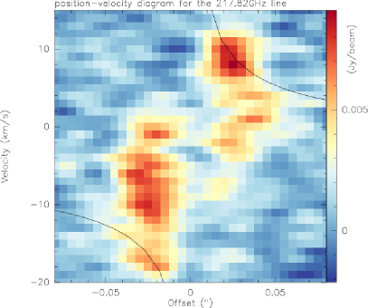
Figure 5: Color-scale shows for mm1 the position-velocity diagram for the line at 217.82 GHz along the axis of the strong velocity gradient visible in Fig. 3. The lines correspond to a Keplerian curve around a 10 M_⊙ central object, not representing the data well.

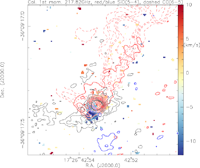
Figure 6: Color-scale shows for mm1 the first moment map (intensity-weighted peak velocities) from the line at 217.82 GHz. The blue and red solid contours present the blue- and redshifted SiO(5-4) emission integrated between [-22,-14] and [0,24] km s^-1, respectively. The red dashed contours show the red-shifted CO(6–5) emission from Beuther et al. (2017b). Blue-shifted CO(6–5) can not be properly imaged in that dataset, most likely because of missing short spacings. The black contours show the lower level 1.3 mm continuum data from the 4$\sigma$ levels of 0.2 mJy beam^-1 to 1.0 mJy beam^-1 in 4$\sigma$ steps.

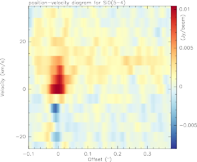
Figure 7: Color-scale shows the position-velocity diagram from SiO(5-4) along the outflow axis seen in Fig. 6.

3.3 Emission lines in other cores

For completeness, we also report detections of emission lines toward a few other sub-sources. We detect line emission from fewer lines toward mm2 and mm12, while all other sub-sources remain undetected in emission lines. Figure 8 presents the first moment maps toward mm1, mm2 and mm12 in the emission line at 232.693 GHz. While for mm1, the velocity structure previously found in the 217.82 GHz line is well recovered, it is interesting that the other two sources also depict clear velocity gradients. The one in mm2 has approximately the same orientation as that in mm1, however, the blue- and red-shifted sides are swapped. For mm12, the velocity gradient is in the northsouth direction. Since we do not have any information about molecular outflows from these two sub-sources mm2 and mm12 (the cm continuum emission from Zapata et al. (2008) is not associated with any of these features either), we cannot infer whether these velocity gradients are caused by rotation, outflows or any other process.

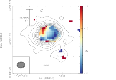
Figure 9: Color-scale shows the first moment map (intensity-weighted peak velocities) from the line at 231.896 GHz for the source mm2. The contours are the 1.3 mm continuum data in $4\sigma$ level of 0.2 mJy beam^-1 up to a 3 mJy beam^-1 level (to avoid too many contours in the center). A scale-bar and the resolution elements of the line (gray) and continuum are shown as well.

For mm2, an additional feature arises when imaging the line at 231.896 GHz (Fig. 9). While the structure in mm1 is the same as found in the other lines, toward mm2 we find emission mainly blue-shifted from the $\varv_{\rm lsr}\sim-3.6$ km s^-1 to $\sim-20$ km s^-1. This emission can either be from the same line, just blue-shifted to high velocities, or it may stem from another spectral line that we cannot differentiate properly. Independent of that, the velocity gradient found in this line is approximately in the northeast-southwest direction, roughly perpendicular to the velocity gradient seen before in the 232.693 GHz line. The perpendicular directions of the velocity gradients in the two lines toward mm2 indicates that one may trace an outflow/jet whereas the other may trace rotation. Since we do not have any additional information at hand, we refrain from further interpretation of these structures.

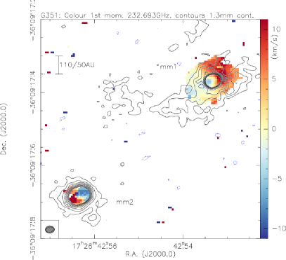
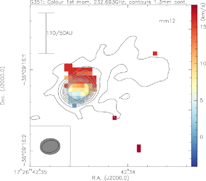
Figure 8: Color-scale shows the first moment maps (intensity-weighted peak velocities) from the line at 232.693 GHz. The left panel focus’ on mm1 and mm2, whereas the right panel presents mm12. The contours are the 1.3 mm continuum data in $4\sigma$ level of 0.2 mJy beam^-1 up to a 3 mJy beam^-1 level (to avoid too many contours in the center). A scale-bar and the resolution elements of the line (gray) and continuum are shown as well.

4 Discussion

4.1 Fragmentation

Fragmentation of molecular clouds and star-forming regions is a hierarchical process, and one finds fragmentation from large-scale molecular clouds (e.g., Blitz 1993; Kramer et al. 1998; McKee & Ostriker 2007; Dobbs et al. 2014) to filament fragmentation from giant 100 pc long filaments (Jackson et al., 2010; Goodman et al., 2014; Ragan et al., 2014; Wang et al., 2014, 2015; Zucker et al., 2015; Abreu-Vicente et al., 2016) to those within star-forming regions (e.g., André et al. 2010, 2014; Hacar et al. 2013; Beuther et al. 2015). It is interesting to note that there seems to be a difference in the dominant process driving the fragmentation of filaments and that of star-forming clumps and cores. While filaments can often be described by self-gravitating cylinders (e.g., Jackson et al. 2010; Kainulainen et al. 2013; Beuther et al. 2015), star-forming regions are often well-described by thermal and/or turbulent Jeans fragmentation (e.g., Palau et al. 2013, 2014; Wang et al. 2014; Beuther et al. 2018, Svoboda et al. in prep.). While previous studies of fragmentation in (high-mass) star-forming regions typically studied the fragmentation of star-forming regions from scales of several 10⁴ au down to scales of a few 1000 au, in this study we now zoom into the most central high-mass star-forming core and investigate the fragmentation on scales of hundreds to 1000 au.

What would be the thermal Jeans fragmentation properties of a typical high-mass core of several 1000 au size? Using the study of the IRAM large program CORE of 20 high-mass star-forming regions, Beuther et al. (2018) find, for regions below 2 kpc distance, typical mean volume number densities between $10^{7}$ and $10^{8}$ cm^-3 averaged over spatial resolution elements of $\sim 0.3^{\prime\prime}-0.4^{\prime\prime}$. Assuming mean temperatures of around 50 K for these regions because the star formation process is already active, we find Jeans lengths between roughly 870 and 2800 au, and Jeans masses between 0.1 and 0.4 M_⊙. Although our observed separations and masses are uncertain due to the poorly constrained distance, projection effects as well as missing flux and optical depth uncertainties, the typical observed source separations and masses (Section 3.1) are on the order of these Jeans estimates.

One may also ask whether all the identified twelve sub-sources will form stars. While the compact structures like mm1, mm2, mm4 or mm12 seem good candidates for actual forming protostars (mm1 is actively driving an outflow, mm2 and mm12 are also showing line emission from highly excited lines), other structures like mm5, mm7 or mm11 appear more diffuse and may simply be local over-densities which could be transient structures and will not form stars within them. In fact, these more diffuse structures may be parts of the otherwise largely filtered out envelope which, if it were infalling, could result in these structures ending up on some protostar later in its evolution.

In this context, the spatial structure of mm9 appears intriguing. Its partly bent and wave-like structure has an appearance similar to gravitationally interacting core structures also observed in recent 3D radiation-hydrodynamical simulations of high-mass star-forming regions (e.g., Meyer et al. 2018; Ahmadi et al. in prep.). For example, Meyer et al. (2018) model an infalling envelope around a self-gravitating disk that evolves while being irradiated by the time-dependent evolution of the central protostar. Independent of their initial angular velocity distribution, all their models form similarly bent-like structures at scales of several hundred to thousand au from the center. From the observational side, infalling streamer-like structures have recently also been reported in other high-mass star-forming regions (e.g., Maud et al. 2017; Izquierdo et al. 2018; Goddi et al. 2018). In particular, the observations and analysis of the high-mass region W33A reveals comparably extended structures at $\sim$1000 au separation from the center that are attributed to spiral-like infalling gas streamer (Maud et al., 2017; Izquierdo et al., 2018). If those data were observed with poorer uv-coverage, these more extended spiral-like structure may well resemble what we see here in G351.77-0.54. Hence, within the G351.77-0.54 region, so far, we do not find a larger disk-like structure like for example in AFGL4176 (Johnston et al., 2015) or G17.64 (Maud et al., 2018), but it is more a multisource environment with smaller-scale structures like those found in W33A or W51n (e.g., Izquierdo et al. 2018; Goddi et al. 2018).

However, with the given data, such interpretation is for G351.77-0.54 still largely premature and speculative. To investigate this “inter-core” gas in more detail, complementary ALMA observations with shorter baselines are needed. With such data, not only can the more diffuse dust emission be studied, but also the line emission at lower brightness to investigate the kinematics of the connecting gas structures.

4.2 Turbulent entrainment

Following the interpretation outlined in Section 3.2 that the compact high-energy line emission stems from the innermost jet/outflow driven from mm1, we can use these data to further analyze the entrainment mechanism. Since large-scale molecular outflows are typically entrained gas and do not directly trace the underlying driving jet, gas entrainment processes are important in the star-formation process. Jet-outflow entrainment processes have been discussed for many years (e.g., Masson & Chernin 1993; Raga et al. 1993; Stahler 1994; Downes & Ray 1999; Arce & Goodman 2002; Cantó et al. 2003; Arce et al. 2007; Frank et al. 2014; Raga 2016). One of the key-diagnostics to study gas entrainment are position-velocity diagrams, and one recurring feature in the literature is the so-called Hubble-law of molecular outflows where the observed gas velocities increase with increasing distance from the source (e.g., Raga et al. 1993; Downes & Ray 1999; Arce et al. 2007). The most discussed outflow entrainment scenarios are turbulent entrainment, jet-bow-shock entrainment as well as wide-angle winds (e.g., Canto & Raga 1991; Masson & Chernin 1993; Stahler 1994; Chernin & Masson 1995; Bence et al. 1996; Cliffe et al. 1996; Li & Shu 1996; Hatchell et al. 1999; Lee et al. 2001; Arce & Goodman 2002; Arce et al. 2007; Frank et al. 2014). A summary of these processes and the corresponding diagnostics, in particular the position-velocity diagrams for the various processes can be found in Arce et al. (2007). While the prompt-entrainment jet-bow-shock models and the wide-angle winds both predict velocity structures where the velocity increases with distance to the source, the more steady-state turbulent entrainment predicts rather the opposite with high velocities close to the source (Fig. 2 in Arce et al. 2007). Interestingly, many outflow studies on larger spatial scales seem to prefer the jet-bow-shock and wide-angle models (e.g., Yu et al. 1999; Lee et al. 2002; Arce & Goodman 2002; Arce et al. 2007; Ray et al. 2007; Tafalla et al. 2017).

However, although the central peak position around mm1 suffers from absorption (e.g., Figs. 1 and 4), our new data of the hot, likely entrained gas around mm1 do not show any Hubble-like velocity structure with increasing velocity away from the center, but we clearly find high-velocity gas very close to the center of the source (Section 3.2, and Figs. 3 and 4). Furthermore, also the position-velocity diagram of SiO(5-4) along the outflow axis exhibits the highest velocities close to the center and then almost constant velocities with increasing distance from the center (Fig. 7). Hence, also out to distances of several hundred au from the center of mm1, the new ALMA long baseline data do not show Hubble-like velocity-structure. We stress that to our knowledge barely any high-mass jet study in thermal line emission so far has ever resolved the scales below 50 au from the driving protostar as we do here (a notable exception is source I in Orion, Ginsburg et al. 2018). Hence, we reach new territory with the supreme capabilities of ALMA. Compared to the basic predictions of the prompt bow-shock entrainment models at the heads of the jets, and the steady-state turbulent entrainment models via Kelvin-Helmholtz instabilities along the jets (e.g., Bence et al. 1996; Arce & Goodman 2002; Arce et al. 2007), on these small scales, the position-velocity diagnostics are more consistent with turbulent entrainment at the jet-outflow interface. From a physical point of view, both processes have to exist, steady-state turbulent entrainment via Kelvin Helmholtz instabilities along the jet-envelope interface as well as prompt entrainment at the head of jets via bow-shocks. Therefore, the question is not that much about the existence of the different processes but rather which of them dominates in one or the other source and at which spatial scales. Hence, the results for G351.77-0.54 do not necessarily contradict previous observational results that found the Hubble-like velocity structure on larger spatial scales. It is rather possible that on the smallest scales, as observed here, turbulent entrainment may be more important whereas on larger scales bow-shock entrainment could become the dominant process. This issue can again only be directly tackled by observations that connect all spatial scales, from those observed in this study of G351.77 to the larger scales of the more typically observed outflows.

An additionally interesting feature with respect to the inner jet/outflow and accretion disk is the extension of the 1.3 mm continuum emission along the axis of the jet/outflow. While elongations of 1.3 mm continuum emission are typically attributed to the dense cores and potential accretion disks, this seems less likely for the case of G351.77-0.54 here. As outlined in Section 3.2 and Fig. 3, while toward the southeast of mm1 the 1.3 mm continuum emission is elongated along the outflow axis, toward the northwest, the mm emission rather resembles a cone-like structure almost enveloping the central SiO(5–4) jet and CO(6–5) outflow emission. While we do not have a reasonable explanation for this asymmetry of the 1.3 mm emission, both features appear qualitatively consistent with entrainment of the ambient dust and gas. It may be that for the blue wing, we see into the outflow lobe and trace the more compact structures, whereas the red wing could cover the central jet better and one would see more of the limb-brightened edges. As discussed in Section 4.1, typical mean densities in these dense cores are $10^{7}$ to $10^{8}$ cm^-3 (e.g., Beuther et al. 2018), and close to the peak positions even higher (Section 3.1). At such high densities, gas and dust are well coupled, and if the gas is entrained by the underlying jet, it should be no surprise that similar spatial structures are also observed in the dust continuum emission.

5 Conclusions

Resolving for one of the first times a high-mass star-forming region at sub-50 au spatial scales (18 or 40 au resolution depending on the distance of 1.0 or 2.2 kpc) reveals various highly interesting outcomes. In the dust continuum emission, we resolve twelve distinct sub-sources within a region of roughly $6^{\prime\prime}\times 6^{\prime\prime}$ or 6000/13200 au at 1.0/2.2 kpc distance. Projected separations between sub-sources range from more than 1000 au to several 100 au but can be even smaller below 100 au. Since we filter out the large-scale emission, very extended structures are not visible in the data, but the largest features we can identify are between approximately 200 and 600 au in size, similar to the size-scales predicted by theoretical simulations for disks around embedded high-mass protostars. Brightness temperatures toward the main continuum peak positions are in excess of 1000 K, indicating high optical depth toward these positions. This high optical depth as well as the missing flux only allows us to derive lower limits for the masses and column densities of the sub-sources. In the hierarchical picture of fragmentation from large-scale clouds to small-scale cores, we find that the fragmentation properties of this high-mass core with a size of several 1000 au is consistent with thermal Jeans fragmentation.

The high continuum optical depth is also confirmed by the fact that most spectral lines toward the dust peak positions are only seen in absorption. However, we find a few lines in emission toward the main source mm1 as well as two other sources mm2 and mm12. Because of the high dust continuum brightness temperatures, these emission lines have to stem from transitions with very high excitation levels $E_{u}/k$ on the order of 1000 K. The emission toward mm1 shows a velocity gradient with the highest velocities found toward the core center. While this high-excitation line emission by itself may be indicative of a Keplerian disk-like structure, additional information let us favor a different interpretation. In particular, the elongation of this velocity gradient is exactly along the direction of the molecular outflow observed in SiO(5–4) and CO(6–5) and perpendicular to the rotational velocity gradient previously identified in 690 GHz CH₃CN$(37_{k}-36_{k})$ data (Beuther et al., 2017b). Hence this gas emission does likely not arise from an inner accretion disk but is more consistent with being caused by the central jet/outflow region. The high-velocity gas close to the center is consistent with steady-state turbulent entrainment of the molecular gas from the underlying jet via Kelvin-Helmholtz instabilities. So far, in G351.77-0.54 we do not identify a larger-scale disk but the region is composed of a smaller-scale multisource environment.

Since this study only covers the smallest spatial scales without any baselines below 55 m, we are not seeing any extended emission. Such extended emission would be important to connect the scales from thousands and more au down to sub-50 au scales observed here. How does the dense compact structure connect to the more extended gas? How are the kinematic connections from large to small spatial scales? These questions can only be addressed by data with a more complete uv-coverage that would trace all spatial scales and would also be sensitive to lower brightness emission from dust and gas. These investigations will be conducted in future studies.