Interpreting BEC in e⁺e^- annihilation

Abstract

The usual interpretation of Bose-Einstein correlations (BEC) of identical boson pairs relates the width of the peak in the correlation function at small relative four-momentum to the spatial extent of the source of the bosons. However, in the $\tau$-model, which successfully describes BEC in hadronic $\mathrm{Z}$ decay, the width of the peak is related to the temporal extent of boson emission. Some new checks on the validity of both the $\tau$-model and the usual descriptions are presented.

1 Introduction

First a brief review of ‘classic’ parametrizations of Bose-Einstein Correlations (BEC) is given and contrasted with the parametrization of the $\tau$-model Tamas;Zimanji:1990 ; ourTauModel . which has been found L3_levy:2011 to describe well Bose-Einstein correlations in hadronic $\mathrm{Z}$ decay.

The data used in this paper are taken from Ref. (L3_levy:2011, ). They comprise both two-jet and three-jet events, as determined using the Durham jet algorithm durham ; durham2 ; durham3 with resolution parameter $y_{\mathrm{cut}}$=0.006, from e⁺e^- annihilation at the $\mathrm{Z}$-pole.

1.1 ‘Classic’ Parametrizations

The Bose-Einstein correlation function, $R_{2}$, is measured by $R_{2}(Q)=\rho(Q)/\rho_{0}(Q)$, where $\rho(Q)$ is the density of identical boson pairs with invariant four-momentum difference $Q=\sqrt{-(p_{1}-p_{2})^{2}}$ and $\rho_{0}(Q)$ is the similar density in an artificially constructed reference sample, which should differ from the data only in that it does not contain the effects of Bose symmetrization of identical bosons. It is often parametrized as

$$R_{2}=\gamma\left[1+\lambda G\right](1+\epsilon Q)\;,$$ (1)

with

$$G=\exp\left(-\left(rQ\right)^{2}\right)\;.$$ (2)

The corresponding distribution of boson emission points in space-time is a spherically symmetric Gaussian with standard deviation $r$.

The factor $(1+\epsilon Q)$ is included to account for non-BEC which are not removed by $\rho_{0}$, i.e., to make up for slight inadequacies in $\rho_{0}$, and $\gamma$ is a normalization parameter. The parameter $\lambda$ is introduced to account for effects reducing the amount of BEC, e.g., some of the bosons coming from resonance decays, or the identical bosons being partially coherent.

However, this description was found L3_levy:2011 not to describe the $\mathrm{Z}$-decay data, a better description being provided by the Edgeworth expansion about the Gaussian L3_3D:1999 :

$$G=\exp\left(-\left(rQ\right)^{2}\right)\cdot\left[1+\frac{\kappa}{3!}H_{3}(rQ)\right]\;,$$ (3)

where $H_{3}$ is the third-order Hermite polynomial.

A different way to depart from the Gaussian is the generalization to a symmetric Lévy stable distribution. Then

$$G=\exp\left(-\left(rQ\right)^{\alpha}\right)\>,$$ (4)

where $0<\alpha\leq 2$ is the so-called index of stability, which was introduced to BEC in Ref. Tamas:Levy2004 .

A fit of the Edgeworth parametrization to the two-jet data of Ref. (L3_levy:2011, ) finds $\kappa=0.71\pm 0.06$, while a fit of the symmetric Lévy parametrization yields $\alpha=1.34\pm 0.04$. Both values are far from the corresponding Gaussian values of $\kappa=0$ and $\alpha=2$, respectively. Although the $\chi^{2}$ of these fits are a great improvement over that of the Gaussian fit, they are still very large. The corresponding confidence levels are $10^{-15}$ for the Gaussian and $10^{-5}$ and $10^{-8}$ for the Edgeworth and Lévy fits, respectively. The symmetric Lévy fit is shown in Fig. 1a.

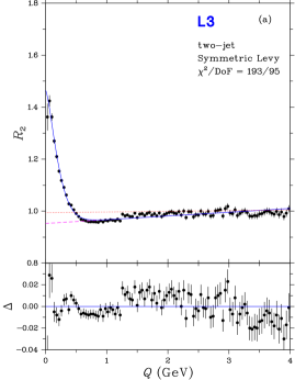
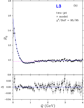
Figure 1: (a) Symmetric Lévy fit for two-jet events; (b) Simplified $\tau$-model fit for two-jet events.

The reason for the failure of the ‘classic’ parametrizations is readily apparent from Fig. 1a. There is a region of anti-correlation ($R_{2}<1$) extending from about $Q=0.5$ to $1.5\,\hbox{$\mathrm{G}$\hbox{$\mathrm{e\kern-1.00006ptV}$}}$. The ‘classic’ parametrizations, which are of the form $1+P$, where $P$ is a positive-definite quantity, are unable to accomadate the anti-correlation. This was not realized for a long time because experiments only plotted the correlation function up to $Q=2\;\hbox{$\mathrm{G}$\hbox{$\mathrm{e\kern-1.00006ptV}$}}$ or less. In Ref. (L3_levy:2011, ) $Q$ was plotted to 4 $\mathrm{G}$$\mathrm{e\kern-1.00006ptV}$, and the anti-correlation became apparent. This anti-correlation, which one might term Bose-Einstein Anti-Correlations (BEAC), as well as the Bose-Einstein correlations (BEC) are both well described by the $\tau$-model.

1.2 The $\tau$-model

The $\tau$-model Tamas;Zimanji:1990 ; ourTauModel rests on several assumptions:

• The average production point is proportional to the momentum of the emitted boson. Dimensionally the momentum must be multiplied by a time divided by a mass to yield a spatial dimension. The description of a two-jet event is invariant to Lorentz boosts along the direction of the colour field. The relevant boost-invariant quantities are the “longitudinal” proper time, $\tau=\sqrt{\overline{t}^{2}-\overline{r}^{2}_{z}}$ and the “transverse” mass, $m_{\mathrm{t}}=\sqrt{E^{2}-p_{z}^{2}}$, resulting in

  $$\overline{x}^{\mu}(p^{\mu})=a\tau\ p^{\mu}\;,\qquad a=1/m_{\mathrm{t}}\;.$$ (5)

• The spatial distribution of production points about their mean is very narrow, although the distribution of proper time may be broad.

• The distribution of $\tau$ is a one-sided Lévy distribution, one-sided because no particles are emitted before the e⁺e^- collision.

Then $R_{2}$ turns out to depend on three variables, $Q$ and the transverse mass of each of the particles making up the pair:

$$R_{2}(Q,a_{1},a_{2}) = \gamma\left\{1+\lambda\cos\left[\frac{\tau_{0}Q^{2}(a_{1}+a_{2})}{2}+\tan\left(\frac{\alpha\pi}{2}\right)\left(\frac{\Delta\tau{Q^{2}}}{2}\right)^{\!\alpha}\frac{a_{1}^{\alpha}+a_{2}^{\alpha}}{2}\right]\right.$$ (6)

$$\hfill\left.\cdot\exp\left[-\left(\frac{\Delta\tau{Q^{2}}}{2}\right)^{\!\alpha}\frac{a_{1}^{\alpha}+a_{2}^{\alpha}}{2}\right]\right\}\cdot\left(1+\epsilon Q\right)\;.$$

Fits in three dimensions are problematic with the available statistics. Hence we simplify this expression by introducing an effective radius, $R$, defined by

$$R=\left(\frac{\Delta\tau}{2}\right)^{\!\alpha}\frac{a_{1}^{\alpha}+a_{2}^{\alpha}}{2}\;.$$ (7)

Further, we assume that particle production begins immediately, i.e., $\tau_{0}=0$. Then

$$R_{2}(Q) =\gamma\left[1+\lambda\cos\left(\left(R_{\mathrm{a}}Q\right)^{2\alpha}\right)\exp\left(-\left(RQ\right)^{2\alpha}\right)\right](1+\epsilon Q)\;,$$ (8a)

$$R_{\mathrm{a}}^{2\alpha} =\tan\left(\frac{\alpha\pi}{2}\right)R^{2\alpha}\;.$$ (8b)

The fit of the simplified $\tau$-model to the two-jet data is shown in Fig. 1b. Unlike the fits of the classic parametrizations, the $\chi^{2}$ is acceptable, and the residuals lack structure.

Note that the difference between the parametrizations of Eqs. (4) and (8) is the presence of the cosine term, which provides the description of the BEAC dip. The parameter $R$ describes the BEC peak, and $R_{\mathrm{a}}$  describes the anti-correlation region. While one might have had the insight to add, ad hoc, a $\cos$ term to Eq. (4), it is the $\tau$-model which provides a physical reason for it and which predicts a relationship, Eq. (8b), between $R$ and $R_{\mathrm{a}}$, i.e., between the correlation and the anti-correlation.

2 Expansions

Recall that the Edgeworth expansion of the Gaussian parametrization provided evidence (in addition to the poor $\chi^{2}$) that the Gaussian was inadequate. In this section we look at expansions of the Symmetric Lévy and the $\tau$-model parametrizations.

2.1 Symmetric Lévy

The symmetric Lévy distribution can be expanded in terms of Lévy polynomials DeKock:WPCF2011 ; Csorgo:Odderon , $l_{i}$, which are orthonormal. The resulting expression for $R_{2}$ is

$$R_{2}(Q)=\gamma\left[1+\lambda\exp\left(-\left|rQ\right|^{\alpha}\right)(1+\sum c_{i}l_{i})\right]\cdot\left(1+\epsilon Q\right)\;.$$ (9)

Fits to the two-jet data are shown in Fig. 2a for orders 0 through 3 of the Lévy polynomials. The order-0 fit (also shown in Fig. 1a) has a very poor $\chi^{2}$, but the order-1 fit has a good $\chi^{2}$. Higher orders show only marginal further improvement.

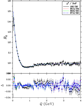
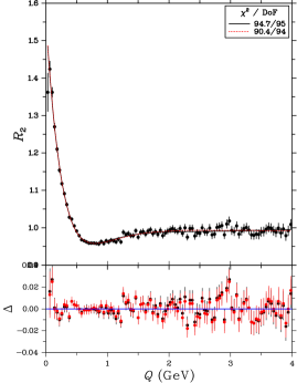
(a)                                                        (b)

Figure 2: (a) Symmetric Lévy fit for two-jet events up to orders 0 through 3 Lévy polynomials; (b) First-order Lévy polynomial fit (black) for two-jet events compared to the $\tau$-model fit (red).

The first-order symmetric Lévy polynomial fit is shown together with the simplified $\tau$-model fit in Fig. 2b. The $\chi^{2}$ of the Lévy polynomial fit is slightly better than the $\tau$-model fit, but the fit curves are nearly identical, what difference there is being mainly for $Q>1.5\,\hbox{$\mathrm{G}$\hbox{$\mathrm{e\kern-1.00006ptV}$}}$.

Comparing Eqs. (8) and (9), we see that in the symmetric Lévy parametrization the cosine of the $\tau$-model parametrization is replaced by the Lévy polynomial expansion. Also, in the exponential $2\alpha$ becomes simply $\alpha$. Fig. 3 compares the cosine and the Lévy polynomials. We see a rather similar behaviour: Both decrease more or less linearly with $Q$, which explains why both fit the data approximately equally well.

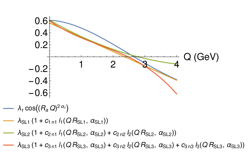
Figure 3: Comparison of the cosine term of the $\tau$-model parametrization with the Lévy polynomial term of the symmetric Lévy parametrization.

2.2 $\tau$-model (asymmetric Lévy)

Lacking an orthogonal polynomial expansion for the asymmetric Lévy distribution $H(\tau)$ of the $\tau$-model, we use, motivated by the results of Ref. (DeKock:WPCF2011, ), a derivative expansion:

$$R_{2}(Q) = {\gamma}\left[1+\lambda\left\{\cos\left(\left(R_{\mathrm{a}}Q\right)^{2\alpha}\right)\exp\left(-\left(RQ\right)^{2\alpha}\right)\right.\right.\qquad\qquad\qquad$$ (10)

$$\left.\left.+\sum c_{n}\frac{{\textrm{d}}^{n}\phantom{Q}}{{\textrm{d}}Q^{n}}\cos\left(\left(R_{\mathrm{a}}Q\right)^{2\alpha}\right)\exp\left(-\left(RQ\right)^{2\alpha}\right)\right\}\right]\cdot\left(1+\epsilon Q\right)\;.$$

We also consider letting $R_{\mathrm{a}}$ be a free parameter rather than as defined in Eq. (8b). The results of these fits are shown in Table 1 and Fig. 4a. The $\chi^{2}$ of the order-1 fit is, of course, smaller than that of the order-0 fit, as is the $R_{\mathrm{a}}$-free fit, and the confidence levels are somewhat better. To test the significance of the improvement in $\chi^{2}$, we make use of the $\chi^{2}$-difference. For the order-0 and order-1 fits this is $\chi^{2}_{\text{diff}}=94.7-90.9=3.8$, and the difference in the number of degrees of freedom is 1. The confidence level for a $\chi^{2}$ of 3.8 with 1 degree of freedom is 5.1%. A small value of this confidence level, say less than 5%, would be grounds for rejecting the order-0 parametrization. (This corresponds to the 95% commonly used in making decisions.) Thus we conclude that for two-jet events the order-0 fit is adequate.

Table 1: Fit results of $\tau$-model parametrizations for two-jet events.

$\begin{array}[]{lccc}\hline\cr&\text{order 0}&\text{order 1}&\text{order 0, $R_{\mathrm{a}}$\ free}\\ \hline\cr\alpha&0.44\pm 0.01&0.43\pm 0.01&0.41\pm 0.02\\ R\ \text{(fm)}&0.78\pm 0.04&0.84\pm 0.05&0.79\pm 0.04\\ R_{\mathrm{a}}\ \text{(fm)}&-&-&0.69\pm 0.04\\ \lambda&0.61\pm 0.03&0.67\pm 0.05&0.63\pm 0.03\\ \gamma&0.979\pm 0.002&0.979\pm 0.002&0.988\pm 0.005\\ \epsilon&0.005\pm 0.001&0.005\pm 0.001&0.001\pm 0.002\\ c_{1}&-&0.0008\pm 0.0005&-\\ \hline\cr\chi^{2}/{\text{DoF}}&94.7/95&90.9/94&91.0/94\\ \text{CL}&49\%&57\%&57\%\\ \hline\cr\end{array}$

The order-0, $R_{\mathrm{a}}$-free fit also provides an adequate description, having a $\chi^{2}$ nearly identical to that of the order-1, $R_{\mathrm{a}}$-constrained fit. Note that the physical parameters ($\alpha$, $R$, $\lambda$) differ at most by about 1 standard deviation in going from order-0 to order-1 or to $R_{\mathrm{a}}$ free. Thus conclusions based on these values, such as the reconstructions of the space-time picture in Ref. (L3_levy:2011, ), remain valid.

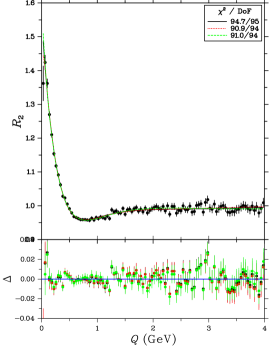
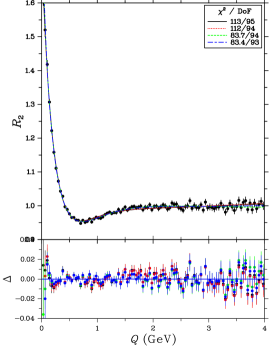
(a)                                                        (b)

Figure 4: (a) Fits of the $\tau$-model (black), the order-1 expansion of the $\tau$-model (red), and the $\tau$-model with $R_{\mathrm{a}}$ free (green), for two-jet events; (b) Fits of the $\tau$-model (black), the order-1 expansion of the $\tau$-model (red), the $\tau$-model with $R_{\mathrm{a}}$ free (green), and the order-1 expansion of the $\tau$-model with $R_{\mathrm{a}}$ free (blue), for three-jet events.

3 Conclusions for two-jet events

We have used expansions about the hypothesized form to test whether it provides an adequate description of the data or is only a (poor) approximation. In the latter case the shape of the expansion terms provide an indication of how to modify the original parametrization. For the symmetric Lévy parametrization this showed that an approximately linearly decreasing function of $Q$ is necessary, which in fact is what is provided by the $\tau$-model.

An expansion in the case of the $\tau$-model is found not to be significant, i.e., the one-sided Lévy distribution of the $\tau$-model is adequate.

4 Three-jet events

For two-jet events hadronization occurs basically in 1+1 dimensions, which lead to the dependence of $R_{2}$ on $\tau$, the longitudinal proper time and $m_{\mathrm{t}}$, the transverse mass. For three-jet events, the $\mathrm{q}$$\bar{\mathrm{q}}$$\mathrm{g}$ system no longer forms a linear system (in the overall centre of mass), but a planar one. There is no event axis by which the transverse mass and longitudinal proper time are defined. Therefore we might expect the $\tau$-model, as formulated for a two-jet system, to work less well.

The results of fits of the $\tau$-model and its first-order expansion, without and with $R_{\mathrm{a}}$ a free parameter, are shown in Fig. 4b and Table 2. Applying the $\chi^{2}$-difference test to the order-0 and order-1 fits yields a confidence level of 37% for the case that $R_{\mathrm{a}}$ is constrained and 58% when $R_{\mathrm{a}}$ is free.

However, the $\chi^{2}$-difference between the order-0 $R_{\mathrm{a}}$ constrained and free cases yields a confidence level of $6\cdot 10^{-8}$. Thus regarding $R_{\mathrm{a}}$ as a free parameter does give significant improvement.

But it must be pointed out that the parameters $R_{\mathrm{a}}$ and $\tau_{0}$ are expected to be highly correlated. While for two-jet events it was found in Ref. (L3_levy:2011, ) that $\tau_{0}$ is consistent with zero, such studies have not yet been performed for three-jet events. Further investigation is ongoing. Also, note that the value of $\alpha$ is significantly less for the fits with $R_{\mathrm{a}}$ free than for those with $R_{\mathrm{a}}$ constrained. This was not the case for two-jet events. This too requires additional investigation.

Table 2: Fit results of $\tau$-model parametrizations for three-jet events.

$\begin{array}[]{lcccc}\hline\cr&\text{order 0}&\text{order 1}&\text{order 0, $R_{\mathrm{a}}$\ free}&\text{order 1, $R_{\mathrm{a}}$\ free}\\ \hline\cr\alpha&0.42\pm 0.01&0.42\pm 0.01&0.35\pm 0.01&0.35\pm 0.01\\ R\ \text{(fm)}&0.98\pm 0.04&0.96\pm 0.05&1.06\pm 0.05&1.00\pm 0.11\\ R_{\mathrm{a}}\ \text{(fm)}&-&-&0.87\pm 0.04&0.96\pm 0.30\\ \lambda&0.84\pm 0.04&0.81\pm 0.05&0.92\pm 0.05&0.65\pm 0.49\\ \gamma&0.977\pm 0.001&0.977\pm 0.001&0.997\pm 0.005&0.994\pm 0.007\\ \epsilon&0.008\pm 0.001&0.008\pm 0.001&0.0003\pm 0.0017&0.001\pm 0.002\\ c_{1}&-&-0.0005\pm 0.0005&-&-0.04\pm 0.08\\ \hline\cr\chi^{2}/{\text{DoF}}&113.2/95&112.4/94&83.7/94&83.4/93\\ \text{CL}&10\%&9\%&77\%&75\%\\ \hline\cr\end{array}$

5 Conclusions for three-jet events

As for the two-jet case, expansion of the $\tau$-model expression does not lead to significant improvement in the fits. This validates the use of an asymmetric Lévy distribution for the longitudinal proper time.

However, significant improvement of the fit is obtained by letting $R_{\mathrm{a}}$ be a free parameter. i.e., by lessening the connection of the simplified $\tau$-model between the BEC peak and the antisymmetric dip. Whether letting $\tau_{0}$ also be a free parameter would also give significant improvement is the subject of ongoing investigation, as is the question whether $\alpha$ decreases as the number of jets increases.

S. Lökös greatfully acknowledges the support from the ERASMUS project of the EU and thanks W. Metzger for his kind hospitality at the Radboud University Nijmegen, The Netherlands. This research was partially supported by the NKTIH FK 123842 and FK 123 959 grants (Hungary), by the Circles of Knowledge Club (Hungary) and by the EFOP 3.6.1-16-2016-00001 project (Hungary).

References

- (1) T. Csörgő, J. Zimányi, Nucl. Phys. A517, 588 (1990)
- (2) T. Csörgő, W. Kittel, W. Metzger, T. Novák, Phys. Lett. B663, 214 (2008)
- (3) L3 Collab., P. Achard, et al., Eur. Phys. J. C71, 1648 (2011)
- (4) Y. Dokshitzer, Contribution cited in Report of the Hard QCD Working Group, Proc. Workshop on Jet Studies at LEP and HERA, Durham, Dec. 1990, J. Phys. g17 (1991) 1537
- (5) S. Catani, et al., Phys. Lett. B269, 432 (1991)
- (6) S. Bethke, et al., Nucl. Phys. B370, 310 (1992)
- (7) L3 Collab., M. Acciarri, et al., Phys. Lett. B458, 517 (1999)
- (8) T. Csörgő, S. Hegyi, W. Zajc, Eur. Phys. J. C36, 67 (2004)
- (9) M. De Kock, H. Eggers, T. Csörgő, in Proc. Workshop on Particle Correlations and Femtoscopy 2011 (PoS, 2011), p. 033
- (10) T. Csörgő, R. Pasechnik, A. Ster, Odderon and proton substructure from a model-independent Lévy imaging of elastic pp and p collisions (2018), ArXiv:1807.02897