Evaluation of Intel Memory Drive Technology Performance for Scientific Applications

Abstract.

In this paper, we present benchmark data for Intel Memory Drive Technology (IMDT), which is a new generation of Software-defined Memory (SDM) based on Intel ScaleMP collaboration and using 3D XPoint ^TM based Intel Solid-State Drives called Optane. We studied IMDT performance for synthetic benchmarks, scientific kernels, and applications. We chose these benchmarks to represent different patterns for computation and accessing data on disks and memory. To put performance of IMDT in comparison, we used two memory configurations: hybrid IMDT DDR4/Optane and DDR4 only systems. The performance was measured as a percentage of used memory and analyzed in detail. We found that for some applications DDR4/Optane hybrid configuration outperforms DDR4 setup by up to 20%.

1. Introduction

In the recent years the capacity of system memory for high performance computing (HPC) systems has not been kept with the pace of the increased central processing unit (CPU) power. The amount of system memory often limits the size of problems that can be solved. System memory is typically based on dynamic random access memory (DRAM). DRAM prices have significantly grown up in the recent year. In 2017, DRAM prices were growing up approximately 10-20% quarterly (tre, 2018). As a result, memory can contribute up to 90% to the cost of the servers.

A modern memory system is a hierarchy of storage devices with different capacities, costs, latencies, and bandwidths intended to reduce price of the system. It makes a perfect sense to introduce yet another level in the memory hierarchy between DRAM and hard disks to drive price of the system down. SSDs are a good candidate because they are cheaper than DRAM up to 10 times. What is more important, over the last 10 years, SSDs based on NAND technology emerged with higher read/write speed and Input/Ouput Operations per Second (IOPS) metric than hard disks.

Recently, Intel announced (Shenoy, 2018) a new SSD product based on novel 3D XPoint^TM technology under the name Intel® Optane^TM. It was developed to overcome the drawbacks of NAND-technology: block-based memory addressing and limited write endurance. To be more specific, with 3D XPoint each memory cell can be addressed individually and write endurance of 3D XPoint memory is significantly higher than NAND SSDs. As a result, 3D XPoint flash memory can be used instead of DRAM, albeit as a slow memory, which can be still an attractive solution given that Intel Optane is notably cheaper than random access memory (RAM) per gigabyte. A novel IMDT allows to use Intel Optane drives as a system memory. Another important advantage of 3D XPoint compared to DRAM is that it has a high density of memory cells, which allows to build compact systems with massive memory banks.

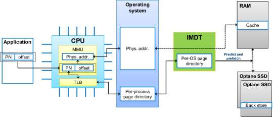
Figure 1. This figure describes how Intel Memory Drive Technology works. Solid lines represent inquiry, dashed lines represent data transfer, and double lines represent commands issued.

In this work, we evaluated the capabilities of Intel Optane drives together with IMDT for numerical simulations requiring large amount of memory. We started with the overview of IMDT technology in section 2. In section 3, we described the methodology. In Sections 4 and 5 we described all benchmarks and corresponding performance results. In section 6 we discussed the performance results, and in Section 7 we presented our conclusions and plans for the future work.

2. Overview of Intel Memory Drive Technology

For effective use of Intel Optane in hybrid RAM-SSD memory systems, Intel corporation and ScaleMP developed a technology called IMDT (imd, 2018a, b). IMDT integrates the Intel Optane into the memory subsystem and makes it appear like RAM to the operating system and applications. Moreover, IMDT increases memory capacity beyond RAM limitations and performs in a completely transparent manner without any changes in operating system and applications. The key feature of IMDT is that RAM is effectively used as cache. As a result, IMDT can achieve good performance compared to all-RAM systems for some applications at a fraction of the cost as we have shown in this paper.

ScaleMP initially has developed a technology to make virtual non-uniform memory access (NUMA) system using high speed node interconnect of modern high performance computational clusters. NUMA systems are typically defined as any contemporary multi-socket system. It allows a processor to access memory at varying degrees of latency or “distance” (e.g. memory attached to another processor), over a network or fabric. In some cases, this fabric is purpose-built for such processor communication, like Intel® QuickPath and UltraPath Interconnects (Intel® QPI and UPI respectively). In other cases, standard fabrics such as Express (PCIe) or Intel® Omni-Path Fabric are used for the same purpose along with software-defined memory (SDM) to provide memory coherency, operating as if additional memory was installed in the system.

Accessing memory at varying lower performance over networks has proven to be feasible and useful by using predictive memory access technologies that support advanced caching and replication, effectively trading latency for bandwidth. This is exactly what IMDT is doing to enable non-volatile memory (NVM) to be used as system memory. Instead of doing it over fabric, however, it does so with storage. With IMDT, most of the Intel Optane capacity is transparently used as an extension to the DRAM capacity of the system.

IMDT is implemented as an operating system (OS)-transparent virtual machine (Figure 1). In IMDT, Intel Optane SSDs are used as part of the system memory to present the aggregated capacity of the DRAM and NVM installed in the system as one coherent, shared memory address space. No changes are required to the operating system, applications, or any other system components. Additionally IMDT implements advanced memory access prediction algorithms to optimize memory access performance.

A popular approach to virtualize disk memory is to store part of virtual memory (VM) pages on special disk partition or file is implemented in all popular operating systems nowadays. However, the resulting performance is very sensitive not only to the storage speed but also to VM manager implementation. It is very important to correctly predict which memory page on disk will be needed soon and to load it in RAM to avoid program spinning in a page fault state. The built-in OS swap in Linux kernel is not very intelligent and usually affected by this problem. On the contrary, IMDT analyzes memory access patterns and prefetches the data into the RAM “cache” (Figure 1) before it is used, resulting in better performance.

IMDT leverage the low-latency media access provide by Intel Optane SSDs. NAND SSD latency cannot be improved by simply aggregating multiple drives. Transitioning to Intel Optane SSDs is another step forward to the reductions of the gap between DRAM and SSD performance by using lower latency media based on the 3D XPoint technology. However, DRAM still has lower latency than Intel Optane, which can potentially affect the performance of applications with DRAM+Optane configuration studied in this paper.

3. Methodology

IMDT architecture is based on the hypervisor layer which manages paging exclusively. This makes a hybrid memory transparent from one side, however, standard CPU counters become unavailable to performance profiling tools. Thus, we took an approach to make a comparison with DRAM-based system side by side. The efficiency metric was calculated as a ratio of software defined performance counters, if available, or simply the ratio of the time-to-solution on DRAM-based system and IMDT-based system.

3.1. Hardware and software configuration

In this study, we used dual-socket Intel Broadwell (Xeon E5 2699 v4, 22 cores, 2.2 GHz) node with latest version of BIOS. We have used two memory configurations for this node. In the first configuration, it was equipped with 256 GB DDR4 registered ECC memory (16$\times$16 GB Kingston 2133 MHz DDR4) and four Intel® Optane^TM SSDs P4800X (320 GB memory mode). We used Intel Memory Drive Technology 8.2 to expand system memory with Intel SSDs up to approximately 1,500 GB. In the second configuration, the node was exclusively equipped by 1,536 GB of DDR4 registered ECC memory (24$\times$64 GB Micron 2666 MHz DDR4). In both configurations we used a stripe of four 400 GB Intel DC P3700 SSD drives as a local storage. Intel Parallel Studio XE 2017 (update 4) was used to compile the code for all benchmarks. Hardware counters on non-IMDT setup were collected using Intel® Performance Counter Monitor (pcm, 2018).

3.2. Data size representation

IMDT assumes that all data is loaded in the RAM before it is actually used. It is important to note that if the whole dataset fits in the RAM, it is very unlikely that it will be moved to the Optane disks. In this case, the difference between IMDT and RAM should be negligible. The difference will be more visible only when the data size is significantly larger than the available RAM. Since the performance results are connected to the actual RAM size, we find more convenient to represent benchmark sizes in parts of RAM in IMDT configuration (256 GB) and not in GB or problem dimensions. Such representation of data sets is more general and the results can be extrapolated to different hardware configurations.

4. Description of Benchmarks

In this section, we described various types of benchmarks to evaluate performance of IMDT. We broadly divided benchmarks in three classes – synthetic benchmarks, scientific kernels, and scientific applications. The goal is to test performance for a diverse set of scientific applications, which have different memory access patterns with various memory bandwidth and latency requirements.

4.1. Synthetic benchmarks

4.1.1. STREAM

(McCalpin, 1995) is a simple benchmark commonly used to measure sustainable bandwidth of the system memory and corresponding computation rate for a few simple vector kernels. In this work, we have used multi-threaded implementation of this benchmark. We studied memory bandwidth for a test requiring $\approx 500$ GB memory allocation on 22, 44, and 88 threads.

4.1.2. Polynomial benchmark

was used to compute polynomials of various degree of complexity. Polynomials are commonly used in mathematical libraries for fast and precise evaluation of various special functions. Thus, they are virtually present in all scientific programs. In our tests, we calculated polynomials of predefined degree over a large array of double precision data stored in memory.

Memory access pattern is similar to the STREAM benchmark. The only difference that we can finely tune the arithmetic intensity of the benchmark by changing the degree of computed polynomials. From this point of view STREAM benchmark is a particular case of the polynomial benchmark when the polynomial degree is zero (STREAM copy) or one (STREAM scale). We used Horner’s method of polynomial evaluation which is efficiently translated to the fused multiply-add (FMA) operations.

We have calculated performance for polynomials of degrees 16, 64, 128, 256, 512, 768, 1024, 2048, and 8192 using various data sizes (from 50 to 900 GB). We studied two data access patterns. In the first one we just read the value from the array of arguments, calculate the polynomial value and add it to a thread-local variable. There is only one (read) data stream to the IMDT disk storage in this case. In another case the result of polynomial calculation updates corresponding value in the array of arguments. There are two data streams here (read and write). Arithmetic intensity of this benchmark was calculated as follows:

(1) $$AI=2\cdot\frac{polynomial\ degree}{sizeof(double)},$$

where factor two corresponds to the one addition and one multiplication for each polynomial degree in Horner’s method of polynomial evaluation.

4.1.3. GEMM

(GEneral Matrix Multiplication) is one of the core routines in Basic Linear Algebra Subprograms (BLAS) library. It is a level 3 BLAS operation defining matrix-matrix operation. GEneral Matrix Multiplication (GEMM) is often used for performance evaluations and it is our first benchmark to evaluate IMDT performance. GEMM is a compute-bound operation with $\mathcal{O}(N^{3})$ arithmetic operations and $\mathcal{O}(N^{2})$ memory operations, where $N$ is a leading dimension of matrices. Arithmetic intensity grows as $\mathcal{O}(N)$ depending on matrix size and is flexible. The source code of the benchmark used in our tests is available here (gem, 2018).

4.2. Scientific kernels

4.2.1. LU decomposition

(where “LU” stands for “lower upper” of a matrix, and also called LU factorization) is a commonly used kernel in a number of important linear algebraic problems like solving system of linear equations, finding eigenvalues, etc. In current study, we used Intel Math Kernel Library (MKL) (mkl, 2018) implementations of LU decomposition, more specifically dgetrf and mkl_dgetrfnpi. We also studied the performance of an LU decomposition algorithm using tile algorithm, which dramatically improved performance of IMDT. The source code of the latter was taken from the hetero-streams code base (het, 2018).

4.2.2. Fast Fourier Transform (FFT)

is an algorithm that samples a signal over a period of time or space and divides it into its frequency components. FFT is an important kernel in many scientific codes. In this work, we have studied the performance of the FFT implemented in MKL library (mkl, 2018). We have used three-dimensional decomposition of the $N\times N\times N$ grid data. The benchmark sizes were $N=(500\div 5800)$ resulting in 0.001-1.5 TB memory footprint.

4.3. Scientific applications

4.3.1. LAMMPS

(Large-scale Atomic/Molecular Massively Parallel Simulator) is a popular molecular simulation package developed in Sandia National Laboratory (Plimpton, 1995). Its main focus is a force-field based molecular dynamics. We have used scaled Rhodopsin benchmark distributed with the source code. Benchmark set was generated from the original chemical system (32,000 atoms) by its periodical replication in $X,Y$ (8 times) and $Z$ (8-160 times) dimensions. The largest chemical system comprises 328,000,000 atoms ($\approx 1.1$ TB memory footprint). Performance metrics – number of molecular dynamics steps per second.

4.3.2. GAMESS

(General Atomic and Molecular Electronic Structure System) is one of the most popular quantum chemistry packages. It is a general purpose program, where a large number of quantum chemistry methods are implemented. We used the latest version of code distributed from GAMESS website (gam, 2018). In this work, we have studied the performance of the Hartree-Fock method. We have used stacks of benzene molecules as a model chemical system. By changing the number of benzene molecules in stack we can vary memory footprint of the application. 6-31G(d) basis set was used in the simulations.

4.3.3. AstroPhi

is a hyperbolic PDE engine which is used for numerical simulation of astrophysical problems (Ast, 2018). AstroPhi realizing a multi-component hydrodynamic model for astrophysical objects interaction. The numerical method of solving hydrodynamic equations is based on a combination of an operator splitting approach, Godunov’s method with modification of Roe’s averaging, and a piecewise-parabolic method on a local stencil (Popov and Ustyugov, 2007, 2008). The redefined system of equations is used to guarantee the non-decrease of entropy (Godunov and Kulikov, 2014) and for speed corrections (A. Vshivkov et al., 2011). The detailed description of a numerical method can be found in (Kulikov et al., 2015). In this work, we used the numerical simulation of gas expansion into vacuum for benchmarking. We have used 3D arrays with up to $2000^{3}$ size ($\approx 1.5$ TB memory footprint) for this benchmark.

4.3.4. PARDISO

is a package for sparse linear algebra calculations. It is a part of Intel MKL library (mkl, 2018). In our work, we studied the performance of the Cholesky decomposition of sparse ($\mathcal{O}(N)$ non-zero elements) $N\times N$ matrices, where $N=(5,10,20,25,30,35,40)\cdot 10^{6}$. Memory footprint of benchmarks varied from 36 to 790 GB.

4.3.5. Intel-QS

(former qHiPSTER) is a distributed high-performance implementation of a quantum simulator on a classical computer, that can simulate general single-qubit gates and two-qubit controlled gates (Smelyanskiy et al., 2016). The code is fully parallelized with MPI and OpenMP. The code is architectured in the way that memory consumption exponentially grows as more qubits are being simulated. We benchmarked a provided quantum FFT test for 30-35 qubit simulations. 35 qubits simulation required more than 1.5TB of memory. The code used in our benchmarks was taken from Intel-QS repository on Github (qsg, 2018).

5. Results

5.1. Synthetic benchmarks

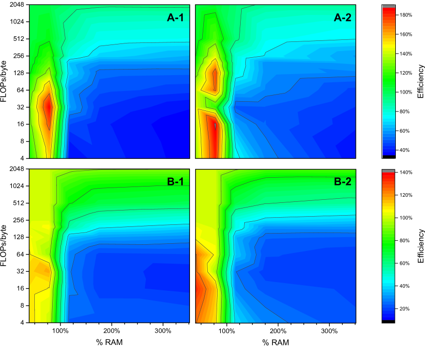
Figure 2. Polynomial benchmark results. (A) – one data stream for 44 (A-1) and 88 (A-2) threads. (B) – two data streams for 44 (B-1) and 88 (B-2) threads. The efficiency is denoted by color with a legend on corresponding row. See text for more details.

5.1.1. STREAM

benchmark was used as a reference to a worst case scenario, where application has low CPU utilization and high memory bandwidth requirements. We obtained 80 GB/s memory bandwidth for the DRAM-configured node, while for IMDT-configured node we got 10 GB/s memory bandwidth for the benchmarks requesting maximum available memory. In other words, we are comparing best case scenario for DRAM bandwidth with the worst case scenario on IMDT. Thus, we can expect the worst possible efficiency of $10/80=12.5\%$ IMDT vs DRAM. It should be noted that running benchmarks which fit in DRAM cache of IMDT results in the bandwidth equal to (80-100 GB/s), which is comparable to the DRAM bandwidth. This is what we expected and it is the proof that IMDT utilizes optimally DRAM cache. The measured bandwidth actually depends only on the number of threads and it was higher for the less concurrent jobs. It applies only to IMDT benchmarks requesting memory smaller than the size of DRAM cache. Memory bandwidth of DRAM-configured node does not depend on the workload size nor on the number of threads.

5.1.2. Polynomial benchmark.

Results of the polynomial benchmarks are presented in Figure 2. As one can see in Figure 2, patterns of efficiency are very similar. If the data fits in the RAM cache of IMDT then IMDT typically shows better performance than DRAM-configured node, especially for short polynomials. High concurrency (88 threads, Figure 2 (A-2 and B-2)) is also beneficial to IMDT in these benchmarks. However, a better efficiency can be obtained for benchmarks with higher order of polynomials. In terms of arithmetic intensity (eq. 1), it is required to have at least 256 floating-point operations per byte to get IMDT efficiency close to $100\%$. It will be discussed later in detail (see Section 5.4).

5.1.3. GEMM benchmark.

According to our benchmarks shown in Figure 3, GEMM shows very good efficiency for every problem size. All observed efficiencies vary from 90% for large benchmarks to 125% for small benchmarks. Such efficiency is expected because GEMM is purely compute bound. To be more specific, the arithmetic intensity even for a relatively small GEMM benchmark is much higher than the required value of 250 FLOP/byte per data stream, which was estimated in polynomial benchmarks. In our tests, we have used custom (“segmented”) GEMM benchmark with improved data locality: all matrices are stored in a tiled format (arrays of “segments”) and matrix multiplication goes tile-by-tile. Thus the arithmetic intensity of all benchmarks is constant and equal to the arithmetic intensity of a simple tile-by-tile matrix multiplication. It is approximately equal to 2 FLOPs multiplied by tile dimension and divided by the size of data type in bytes (4 for float and 8 for double). In our benchmark with a single-precision GEMM with typical tile dimension size of $\approx$43000, the arithmetic intensity is $\approx$21500 FLOPs/byte, which is far beyond the required 250 FLOPs/byte.

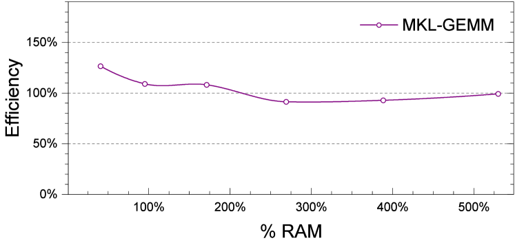
Figure 3. IMDT efficiency plot for GEMM benchmark. Higher efficiency is better. 100% efficiency corresponds to DRAM performance.

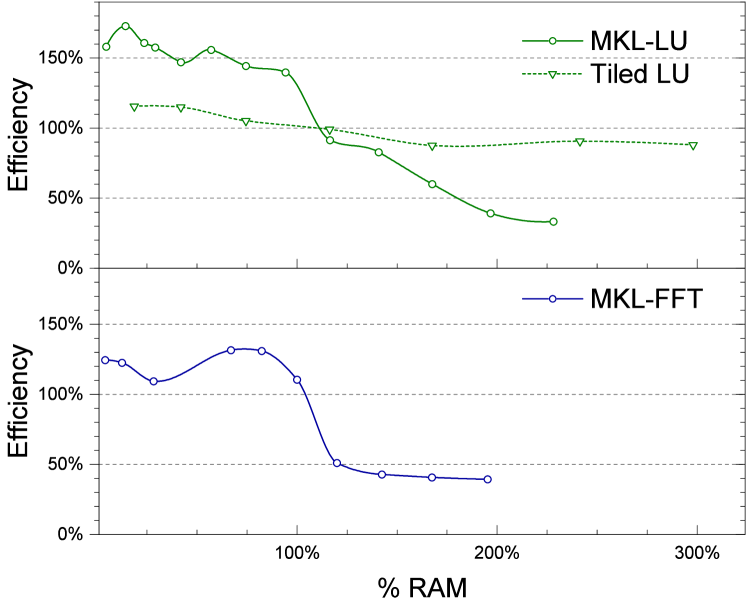
Figure 4. IMDT efficiency plots for LU and FFT benchmarks. Two implementations (MKL and tiled) of LU decomposition were benchmarked. Higher efficiency is better. 100% efficiency corresponds to DRAM performance.

5.2. Scientific kernels

5.2.1. LU decomposition

The efficiency of LU decomposition implemented in MKL library strongly depends on the problem size. The efficiency is excellent when a matrix fits into the memory (Figure 4). We observe about $150\%-180\%$ speedup on IMDT for small matrices. However, the efficiency decreases down to $\approx 30\%$ for very large matrices with leading dimension equal or greater than $\approx 2\cdot 10^{5}$. This result was unexpected; in fact, our LU implementation calls BLAS level 3 functions such as GEMM, which has excellent efficiency on IMDT as we demonstrated in previous section. We can provide two explanations for unfavorable memory access patterns in LU decomposition. First one is the partial pivoting which interchanges rows and columns in the original matrix. Second, matrix is stored as a contiguous array in memory that is known for its inefficient memory access to the elements of the neighboring columns (rows in case of Fortran). Both problems are absent in a special tile-based LU decomposition benchmark implemented in hetero-streams code base. We also ran benchmarks for this optimized LU decomposition benchmark. Tiling of the matrix not only improved the performance by about 20% for both “DRAM” and “IMDT” memory configurations, but also improved the efficiency of IMDT to $\approx$90% (see Figure 4). Removing of pivoting only without introducing matrix tiling does not significantly improve the efficiency of LU decomposition.

5.2.2. Fast Fourier Transform.

The results of MKL-FFT benchmark are similar to those obtained for MKL-LU as shown in Figure 4. For small problem sizes the efficiency of IMDT exceeds $100\%$, but for large benchmarks the efficiency drops down to $\approx 40\%$. Performance drop occurs at $100\%$ of RAM utilization. FFT problems typically have relatively small arithmetic intensity (small ratio of FLOPs/byte). Thus, obtaining relatively low IMDT efficiency was expected. We still believe that the FFT benchmark can be optimized for memory locality to improve IMDT efficiency even higher (see (Bailey, 1989; Cormen and Nicol, 1998; Akin et al., 2016) for the examples of memory-optimized FFT implementations).

5.3. Scientific applications

The benchmarking results for different scientific applications are shown in Figure 5 and Figure 6. The applications are PARDISO, AstroPhi, LAMMPS, Intel-QS, and GAMESS. All applications except PARDISO show similar efficiency trends. When a benchmark requests memory smaller than the amount of available DRAM, the application performance on the IMDT-configured node is typically higher than for DRAM-configured node. At a certain threshold, which is typically a multiple of DRAM size, the IMDT efficiency declines based on the CPU Flop/S and memory bandwidth requirements.

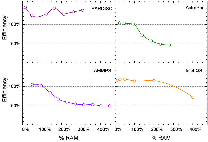
Figure 5. IMDT efficiency plots for various scientific applications. Higher efficiency is better. 100% efficiency corresponds to DRAM performance.

5.3.1. MKL-PARDISO

PARDISO is very different from other studied benchmarks. The observed IMDT efficiency is 120-140% of “DRAM”-configured node for all studied problem sizes. It was not very surprising because Cholesky decomposition is known to be compute intensive. MKL-PARDISO is optimized for the disk-based out-of-core calculations resulting in excellent memory locality to access data structures. As a result, this benchmark always benefits from faster access to the non-local NUMA memory on IMDT which results in the improved performance on “IMDT”-configured node.

5.3.2. AstroPhi

In Figure 5 we presented the efficiency plot of Lagrangian step of the gas dynamic simulation, which is the most time consuming step ($>90\%$ compute time). This step describes the convective transport of the gas quantities with the scheme velocity for the gas expansion into vacuum problem. The number of FLOPs/byte is not very high and the efficiency plot follows the trend we described above. We observe a slow decrease in efficiency down to $\approx$50% when the data does not fit into DRAM cache of IMDT. Otherwise the efficiency is close to 100%.

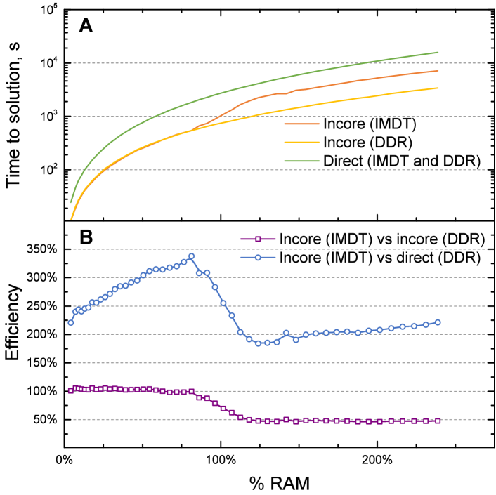
Figure 6. GAMESS Hartree-Fock simulation (10 iterations) for stacks of benzene molecules with 6-31G(d) basis set. (A) Time to solution in seconds, lower is better. (B) IMDT efficiency, higher efficiency is better, 100% efficiency corresponds to DRAM performance. The performance of the direct Hartree-Fock on “IMDT” and “DRAM”-configured node (see text for details) is the same ((A), green line).

5.3.3. LAMMPS

We studied the performance of the molecular dynamics of the Rhodopsin benchmark provided with LAMMPS distribution. It is an all-atom simulation of the solvated lipid bilayer surrounding Rhodopsin protein. The calculations are dominated by the long-range electrostatics interactions in particle-particle mesh algorithm. The results of benchmarks are presented in Figure 5. It is obvious that LAMMPS efficiency follows the same pattern as AstroPhi and FFT: it is more than 100% when tests fit in the DRAM cache of the IMDT and it is dropping down when tests do not fit. For tests with high memory usage the efficiency is $\approx$50%.

5.3.4. Intel-QS

We benchmarked Intel-QS using provided quantum FFT example for 30-35 qubits. Actually, each additional qubit doubles the amount of memory required for the job. For that reason we had to stop at 35 qubit test which occupy about 1 TB of memory. The observed IMDT efficiency was greater than 100% for 30-34 qubits and drops down to $\approx$70% at 35 qubit simulation. A significant portion of the simulation take FFT steps. Thus, degradation of the performance at high memory utilization was not surprising. However, the overall efficiency is almost two times better than for FFT benchmark.

5.3.5. GAMESS

We studied the performance of the two Hartree-Fock method (HF) algorithms. HF is solved iteratively and for each iteration a large number of electron-repulsion integrals need to be re-computed (direct HF) or read from disk or memory (conventional HF). In the special case of conventional HF called incore HF, ERIs are computed once before HF iterations and stored in DRAM. In the subsequent HF iterations, the computed ERIs are read from memory. We benchmarked both direct and incore HF methods. The former algorithm has small memory footprint, but re-computation of all ERIs each iteration (typical number of iterations is 20) results in much longer time to solution compared to incore HF method if ERIs fit in memory.

The performance of the direct HF method on “DRAM” and “IMDT”-configured nodes is very similar (see Figure 6 (A), green line). However, the performance of the incore method differs between “DRAM” and “IMDT” (see Figure 6 (A), red and yellow lines). The efficiency shown in Figure 6 (B) for incore IMDT vs incore DRAM (purple line) behaves similar to other benchmarks – when benchmarks fits in the DRAM cache of the IMDT then the efficiency is close to 100%, otherwise it decreases to $\approx$50%. But for incore IMDT vs direct DRAM (blue line) the efficiency is much better. The efficiency varies between approximately 200% and 350%. Thus, IMDT can be used to speed up Hartree-Fock calculations when the amount of DRAM is not available to fit all ERIs in memory.

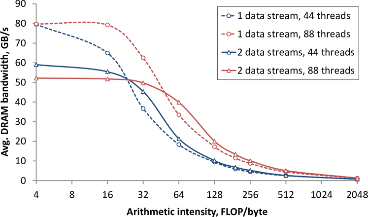
Figure 7. Average DRAM bandwidth in the polynomial benchmark depending on the arithmetic intensity (polynomial degree), number of data streams (1 data stream – read-only access pattern, 2 data streams – read/write access pattern, see text for details), and the number of working threads. The results were obtained by Intel Processor Counter Monitor (sum of System READ and WRITE counters).

5.4. Analysis of IMDT performance

Modern processors can overlap data transfer and computation very efficiently. A good representative example is the Polynomial benchmark (see Section 4.1.2). When the polynomial degree is low the time required to move data from system memory to CPU is much higher than the time of polynomial computation (Section 5.1.2, Figure 2). In this case, the performance is bound by memory bandwidth. By increasing the amount of computation, the overlap between data transfer and computation becomes more efficient and the benchmark gradually transforms from a memory-bound to a compute-bound problem. Increasing of arithmetic intensity is achieved by increasing the degree of polynomials (see eq. 1).

On Figure 7 the dependence of average DRAM bandwidths on the arithmetic intensity is shown for polynomial benchmarks with different number of data streams. The improvement of overlap between data transfer and computation is observed at about 16-32 FLOP/byte. The computation of low-order polynomials (less than 16 FLOP/byte) is not limited by the compute power, resulting in high memory bandwidth. The bandwidth value depends on I/O pattern (i.e. the number of data streams) and it is limited by the DRAM memory bandwidth, which is about 80 GB/s.

The bandwidth dependence on the number of data streams of low-order polynomials results from NUMA memory access. If the benchmark was optimized for NUMA, the highest bandwidth for one and two data streams would be the same. However, in IMDT architecture, while application thread accesses the remote NUMA node for writes, IMDT places the data to the DRAM attached to the local NUMA node. This can significantly reduce the pressure on the cross-socket link and as a result the performance can become better than DRAM based system performance. It is exactly what we observed in our tests when all the data fits in the DRAM cache (see Figure 2).

When the arithmetic intensity grows beyond 16 FLOP/byte, the memory bandwidth starts decreasing. At 64 FLOP/byte and beyond the benchmark becomes compute bound. It means that the memory bandwidth does not depend on the number of data streams but on the availability of computational resources (i.e. number of threads). However, the memory bandwidth decreases slowly with the arithmetic intensity (Figure 7). Taking into account that the memory bandwidth of our IMDT system is capped by 10 GB/s, we expect that only those benchmarks that are below this threshold will have good efficiency. It is expected that it will apply to all benchmarks with different problem sizes. In terms of the arithmetic intensity, it corresponds to $\approx 128-256$ FLOP/byte. This correlation is shown on Figure 2. The same analysis can be applied to any benchmark to estimate the potential efficiency of the IMDT approach.

5.5. Summary

To sum up our benchmarking results, our tests show that there is virtually no difference between using DRAM and IMDT if a benchmark requires memory less than the amount of available RAM. IMDT correctly handles these cases, if the test fits in RAM and there is no need to use Optane memory. In fact, IMDT frequently outperforms RAM because IMDT has advanced memory management system. The situation is very different for large tests. For some tests like dense linear algebra, PARDISO and Intel-QS efficiency remains high, while for other applications like LAMMPS, AstroPhi, and GAMESS the efficiency slowly declines to about 50%. Even in the latter case IMDT can be attractive for scientific users since it enables larger problem sizes to be addressed.

6. Discussion

One of the most important benefits of IMDT is that it significantly reduces data traffic trough Intel QuickPath Interconnect (QPI) bus on NUMA systems. For example, GEMM unoptimized benchmark on “DRAM”-configured node performs about 20-50% slower for large datasets compared to a small ones. The main reason is overloaded QPI bus. When a benchmark saturates QPI bandwidth then it causes CPU stalls waiting for data. QPI bandwidth in our system is 9.6 GT/s (1 GT/s$=10^{9}$ transfers per second) or $\approx$10 GB/s unidirectional ($\approx$20 GB/s bidirectional) and it can easily become a bottleneck. It is an inherent issue of multisocket NUMA-systems which adversely affects performance of not only GEMM, but any other applications.

There are a few ways to resolve this issue. For example, in optimized GEMM implementation (gem, 2018) matrices are split to tiles, which are placed in memory intelligently taking into the account the “first-touch” memory allocation policy in Linux OS. As a result, QPI bus load drops to 5-10% and performance significantly improves achieving almost theoretical peak. It was observed in our experiments with GEMM by using Intel Performance Counter Monitor (PCM) software (pcm, 2018).

There is no such issue with IMDT and performance is consistently close to theoretical peak even for the unoptimized GEMM implementation. IMDT provides optimal access to the data on the remote NUMA node improving the efficiency of almost all applications. This is why we almost never seen in practice a very low IMDT efficiency even for strongly memory-bandwidth bound benchmarks like FFT and AstroPhi. Theoretical efficiency minimum of 12.5% was observed only for the specially designed synthetic benchmarks like STREAM and polynomial benchmark.

However, IMDT is not a solution to all memory-related issues. For example, it cannot help in situations when an application has random memory access patterns across a large number of memory pages with a low degree of application parallelism. While the performance penalty is not very high for DRAM memory, frequent access of the IMDT backstore on SSD can be limited by the bandwidth of Intel Optane SSD, and IMDT can only compensate for that if the workload has a high degree of parallel memory accesses (using many threads or many processes concurrently). In such cases, it may be beneficial to redesign data layout for better locality of data structures. In this work, we observed it when we ran MKL implementation of LU decomposition. Switching to the tiled implementation of the LU algorithm results in the significantly improved efficiency of IMDT because of better data locality. The similar approach can be applied to other applications. However, it is beyond the scope of this paper and it is a subject for our future studies.

7. Conclusions and future work

IMDT is a revolutionary technology that flattens the last levels of memory hierarchy: DRAM and disks. One of the major IMDT advantages is the high density of memory. It will be feasible in the near future to build systems with many terabytes of Optane memory. In fact, the bottleneck will not be the amount of Optane memory, but the amount of available DRAM cache for IMDT. It is currently possible to build an IMDT system with 24 TB of addressable memory (with 3 TB DRAM cache), which is not possible to build with DRAM. Even if it was possible to build a such system, IMDT offers a more cost effective solution.

There are HPC applications with large memory requirements. It is a common practice for such applications to store data in parallel network storage or use distributed memory. In this case, the application performance can be limited by network bandwidth. There is now another alternative which is to use DRAM+Optane configuration with IMDT. In theory, the bandwidth of the multiple striped Optane drives exceeds network bandwidth. IMDT especially benefits the applications that poorly scale on the multi-node environment due to high communication overhead. A good example of such application is a quantum simulator. Indeed, Intel-QS simulator efficiency shown in Figure 5 is excellent compared to other applications. Another good application that fits profile is the visualization of massive amount of data. We plan to explore the potential of IMDT for such applications in our future work.

IMDT prefetching subsystem analyzes memory access patterns in the real time and makes appropriate adjustments according to workload characteristics. This feature is crucial for IMDT performance and differentiates it from other solutions such as OS swap. We plan to analyze it in detail in our future work.

This work is important because we systematically studied performance of IMDT technology for a diverse set of scientific applications. We have demonstrated that applications and benchmarks exhibit reasonable performance level, when the system main memory is extended with the help of IMDT by Optane SSD. In some cases, we have seen DRAM+Optane configuration to outperform DRAM-only system by up to 20%. Based on performance analysis, we provide recipes how to unlock full potential of IMDT technology. It is our hope that this work will educate professionals about this new exciting technology and promote its wide-spread use.

8. Acknowledgements

This research used the resources of the Argonne Leadership Computing Facility, which is a U.S. Department of Energy (DOE) Office of Science User Facility supported under Contract DE-AC02-06CH11357. We gratefully acknowledge the computing resources provided and operated by the Joint Laboratory for System Evaluation (JLSE) at Argonne National Laboratory. We thank the Intel® Parallel Computing Centers program for funding, ScaleMP team for technical support, RSC Group and Siberian Supercomputer Center ICMMG SB RAS for providing access to hardware, and Gennady Fedorov for help with Intel® PARDISO benchmark. This work was partially supported by the Russian Fund of Basic Researches grant 18-07-00757, 18-01-00166 and by the Grant of the Russian Science Foundation (project 18-11-00044).

References

- (1)
- Ast (2018) 2018. AstroPhi. The hyperbolic PDE engine . https://github.com/IgorKulikov/AstroPhi
- het (2018) 2018. Hetero Streams Library. https://github.com/01org/hetero-streams
- mkl (2018) 2018. Intel Math Kernel Library. https://software.intel.com/mkl
- imd (2018a) 2018a. Intel Memory Drive Technology. https://www.intel.com/content/www/us/en/software/intel-memory-drive-technology.html
- pcm (2018) 2018. Intel Performance Counter Monitor – A better way to measure CPU utilization. www.intel.com/software/pcm
- gem (2018) 2018. Segmented SGEMM benchmark for large memory systems. https://github.com/ScaleMP/SEG_SGEMM
- imd (2018b) 2018b. Software Defined Memory at a Fraction of the DRAM Cost – white paper. https://www.intel.com/content/www/us/en/solid-state-drives/intel-ssd-software-defined-memory-with-vm.html
- gam (2018) 2018. The General Atomic and Molecular Electronic Structure System (GAMESS). http://www.msg.ameslab.gov/gamess/index.html
- qsg (2018) 2018. The Intel Quantum Simulator. https://github.com/intel/Intel-QS
- tre (2018) 2018. TrendForce. http://www.trendforce.com
- A. Vshivkov et al. (2011) Vitaly A. Vshivkov, Galina G. Lazareva, Alexei V. Snytnikov, I Kulikov, and Alexander V. Tutukov. 2011. Computational methods for ill-posed problems of gravitational gasodynamics. 19 (05 2011).
- Akin et al. (2016) Berkin Akin, Franz Franchetti, and James C. Hoe. 2016. FFTs with Near-Optimal Memory Access Through Block Data Layouts: Algorithm, Architecture and Design Automation. J. Signal Process. Syst. 85, 1 (Oct. 2016), 67–82. https://doi.org/10.1007/s11265-015-1018-0
- Bailey (1989) D. H. Bailey. 1989. FFTs in External of Hierarchical Memory. In Proceedings of the 1989 ACM/IEEE Conference on Supercomputing (Supercomputing ’89). ACM, New York, NY, USA, 234–242. https://doi.org/10.1145/76263.76288
- Cormen and Nicol (1998) Thomas H Cormen and David M Nicol. 1998. Performing out-of-core FFTs on parallel disk systems. Parallel Comput. 24, 1 (1998), 5–20.
- Godunov and Kulikov (2014) S. K. Godunov and I. M. Kulikov. 2014. Computation of discontinuous solutions of fluid dynamics equations with entropy nondecrease guarantee. Computational Mathematics and Mathematical Physics 54, 6 (01 Jun 2014), 1012–1024. https://doi.org/10.1134/S0965542514060086
- Kulikov et al. (2015) I.M. Kulikov, I.G. Chernykh, A.V. Snytnikov, B.M. Glinskiy, and A.V. Tutukov. 2015. AstroPhi: A code for complex simulation of the dynamics of astrophysical objects using hybrid supercomputers. Computer Physics Communications 186, Supplement C (2015), 71 – 80. https://doi.org/10.1016/j.cpc.2014.09.004
- McCalpin (1995) John D. McCalpin. 1995. Memory Bandwidth and Machine Balance in Current High Performance Computers. IEEE Computer Society Technical Committee on Computer Architecture (TCCA) Newsletter (Dec. 1995), 19–25.
- Plimpton (1995) Steve Plimpton. 1995. Fast Parallel Algorithms for Short-Range Molecular Dynamics. J. Comput. Phys. 117, 1 (1995), 1–19. https://doi.org/10.1006/jcph.1995.1039
- Popov and Ustyugov (2007) M. V. Popov and S. D. Ustyugov. 2007. Piecewise parabolic method on local stencil for gasdynamic simulations. Computational Mathematics and Mathematical Physics 47, 12 (01 Dec 2007), 1970–1989. https://doi.org/10.1134/S0965542507120081
- Popov and Ustyugov (2008) M. V. Popov and S. D. Ustyugov. 2008. Piecewise parabolic method on a local stencil for ideal magnetohydrodynamics. Computational Mathematics and Mathematical Physics 48, 3 (01 Mar 2008), 477–499. https://doi.org/10.1134/S0965542508030111
- Shenoy (2018) Navin Shenoy. 2018. What Happens When Your PC Meets Intel Optane Memory? https://newsroom.intel.com/editorials/what-happens-pc-meets-intel-optane-memory/
- Smelyanskiy et al. (2016) M. Smelyanskiy, N. P. D. Sawaya, and A. Aspuru-Guzik. 2016. qHiPSTER: The Quantum High Performance Software Testing Environment. ArXiv e-prints (Jan. 2016). arXiv:quant-ph/1601.07195 https://arxiv.org/abs/1601.07195v2