The next-to-leading order corrections to $\rho$ meson electromagnetic form factors in the $k_{T}$ factorization approach

Abstract

In this paper we calculate the next-to-leading-order (NLO) corrections to $\rho$-meson electromagnetic form factors by employing the $k_{T}$ factorization approach. We find that the NLO correction to $F_{i}(Q^{2})(i=LT,TL)$ is around $30\%$ of the leading-order (LO) contribution in the region $Q^{2}>2GeV^{2}$. The NLO correction to $F_{LL}(Q^{2})$ is close to $20\%$ of the LO one in the region $Q^{2}>3GeV^{2}$. The NLO radiative corrections to the electric, magnetic, and quadruple form factors $F_{j}(Q^{2})(j=1,2,3)$ are sizeable in magnitude and agree with those from other approaches.

I Introduction

The form factors, as the important nonperturbative observables in hadron physics, are essential for studying the structure of various hadrons. For light meson, their electromagnetic and transition form factors have been studied extensively due to their significance in phenomenology. Over the past decades, the collinear and $k_{T}$ factorization for light meson form factors have been demonstrated pi2 ; Nagashima2 ; Nagashima3 ; rhopi ; rho ; Brho and calculatedpipi2 ; pipi3 ; rholo ; rhopinlo based on the Perturbative QCD (PQCD) factorization approach. For the pseudoscalar mesons such as the pion, the form factors are well understood up to NLO accuracy pipi2 ; pipi3 . For the vector mesons, however, the situation is rather different. For the $\rho$ meson, for example, the NLO correction to its electromagnetic form factor in $k_{T}$ factorization is still absent now. In early years, the NLO correction to $\rho$-meson electromagnetic form factors have been investigated by employing the QCD sum rulesBraguta , and the light cone sum rulesAliev ,the light-front quark model Ho-Meoyng , lattice calculate W. Andersen and so on. In this paper, we will calculate the NLO correction to the $\rho$-meson electromagnetic form factors associated with the process $\rho\gamma^{*}\to\rho$ in the framework of the $k_{T}$ factorization approach.

A modified perturbative QCD approach based on the $k_{T}$ factorization, named as the PQCD approach Brodsky ; Huang ; Li381 ; Botts ; StermanAJ ; YuHP ; ZuoHZ , was proposed two decades ago and has been successfully applied for many exclusive processes, such as the calculations of some transition form factors Zhang2014 , the two body and three body decays of B meson wang2016 ; Rui2018 ; Ya2017 ; Ma2017 ; Qin:2014xta , the production of light mesons in colliders Lu:2018obb and so on. By introducing a small transverse momentum $k_{T}$, the infrared divergences could be regulated in both the full QCD Feynman diagrams and the effective diagrams. Both the large double logarithms could be absorbed by the resummation technology. The light-cone singularities are regularized by rotating the Wilson lines away from the light cone collins ; J.P. Ma . The physical amplitudes then can be written as the convolution of the universal nonperturbative hadron wave functions and a hard scattering kernel. For the $\rho$ meson electromagnetic form factor, its NLO hard kernel is defined as the difference between the full QCD Feynman diagrams and the corresponding effective ones in $k_{T}$ factorization theorem. In the transition process, the collinear divergence from gluon emission in the quark diagrams are cancelled by those divergences in the $\rho$ effective wave function, and the soft divergences will be canceled by summing over all quark diagrams, which ensured by the KLN theorem Lee:1964is ; Kinoshita:1962ur . Then we can derive the infrared-safe $k_{T}$-dependent NLO hard kernel for $\rho$-meson electromagnetic form factors in the $k_{T}$ factorization approach, which setting the renormalization and factorization scales as the internal hard scale.

This paper is organized as follows. In Sec. II, we calculate the $O(\alpha_{s}^{2})$ QCD quark diagrams, and effective diagrams for rho wave function, and then derive the NLO hard kernel for its electromagnetic form factor. Numerical results are performed in Sec. III. Sec. IV contains the conclusion.

II THEORETICAL FRAMEWORK

In this section we consider the NLO gluon radiative corrections to the rho meson electromagnetic form factors in the framework of the $k_{T}$ factorization. The moment of initial-state (final-state) $\rho$ meason is defined in the light-cone (LC) coordinate as,

$$p_{1}=\frac{Q}{\sqrt{2}}(1,r^{2}_{\rho},0),\,\,\,\,\,\ p_{2}=\frac{Q}{\sqrt{2}}(r^{2}_{\rho},1,0),$$ (1)

where $Q^{2}=2P_{1}\cdot P_{2}$ is the momentum transfer squared from the virtual photon, and the dimensionless factor $r^{2}_{\rho}$ is $r^{2}_{\rho}\equiv M^{2}_{\rho}/Q^{2}$. The anti-quark in initial and final pion carries momentum $k_{1}=(x_{1}p^{+}_{1},0,\mathbf{k_{1T}})$ and $k_{2}=(0,x_{2}P^{-}_{2},\mathbf{k_{2T}})$, respectively, $\mathbf{k_{T}}$ represents the transversal momentum, and x is parton momentum fraction. The polarization vectors of the initial and final $\rho$ meson are also defined as,

$$\epsilon_{1\mu}(L)=\frac{1}{\sqrt{2}r_{\rho}}(1,-r_{\rho}^{2},\mathbf{0_{T}}),\,\,\,\,\ \epsilon_{1\mu}(T)=(0,0,\mathbf{1_{T}}),$$

$$\epsilon_{2\mu}(L)=\frac{1}{\sqrt{2}r_{\rho}}(-r_{\rho}^{2},1,\mathbf{0_{T}}),\,\,\,\,\ \epsilon_{2\mu}(T)=(0,0,\mathbf{1_{T}}).$$ (2)

The LO quark diagrams are shown in Fig. 1. We focus on Fig. 1(a) only, since the contribution from other three diagrams can be obtained from the exchanging symmetry between Fig. 1(a) and Figs. 1(b-d).

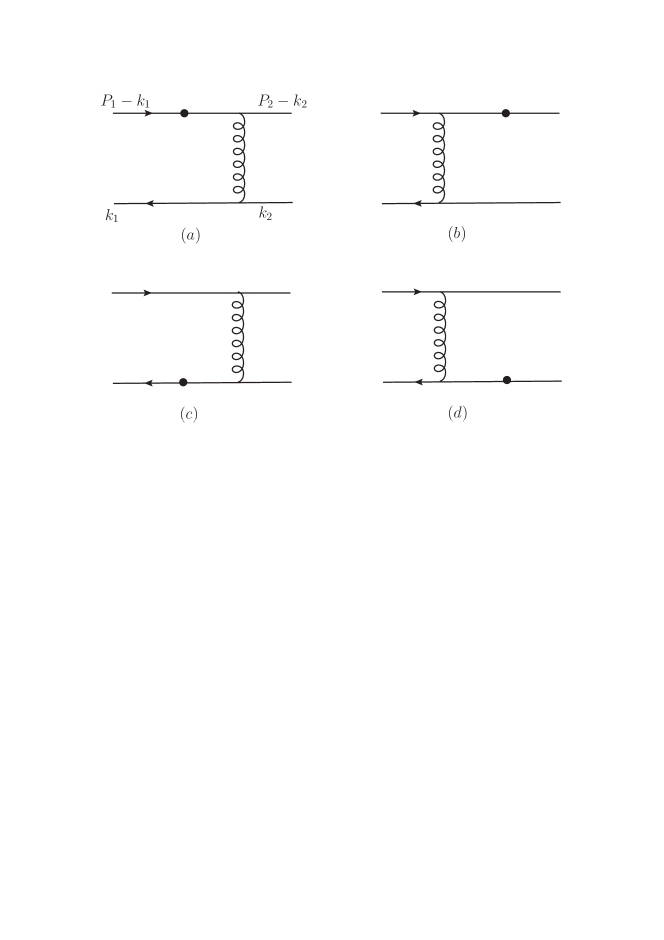
Figure 1: The leading order Feynman diagrams for $\rho\gamma^{\star}\rightarrow\rho$ process.

The related meson wave functions are written as in Refs. Ball:1998sk ; Ball:1998ff ,

$$\langle 0|\bar{u}(0)_{j}d(z_{1})_{l}|\rho^{-}(p_{1},\epsilon_{1T})\rangle=\frac{1}{\sqrt{2N_{C}}}\int_{0}^{1}dx_{1}e^{ix_{1}p_{1}z_{1}}\left\{p/_{1}\epsilon/_{1T}\phi_{\rho}^{T}(x_{1})+m_{\rho}\epsilon/_{1T}\phi^{v}_{\rho}(x_{1})\right.$$

$$\left.\hskip 227.62204pt+m_{\rho}i\epsilon_{\mu\nu\rho\sigma}\gamma^{\mu}\gamma_{5}\epsilon^{\nu}_{1T}n^{\rho}v^{\sigma}\phi_{\rho}^{a}(x_{1})\right\}_{lj},$$ (3)

$$\langle 0|\bar{u}(0)_{j}d(z_{1})_{l}|\rho^{-}(p_{1},\epsilon_{1L})\rangle=\frac{1}{\sqrt{2N_{C}}}\int_{0}^{1}dx_{1}e^{ix_{1}p_{1}z_{1}}\left\{M_{\rho}\epsilon/_{1L}\phi_{\rho}(x_{1})+\epsilon/_{1L}p/_{1}\phi^{t}_{\rho}(x_{1})\right.$$

$$\left.\hskip 227.62204pt+M_{\rho}\phi_{\rho}^{s}(x_{1})\right\}_{lj},$$ (4)

$$\langle\rho^{+}(p_{2},\epsilon_{2T})|\bar{u}(z_{2})_{j}d(0)_{l}|0\rangle=\frac{1}{\sqrt{2N_{C}}}\int_{0}^{1}dx_{2}e^{ix_{2}p_{2}z_{2}}\left\{\epsilon/_{2T}p/_{2}\phi_{\rho}^{T}(x_{2})+m_{\rho}\epsilon/_{2T}\phi^{v}_{\rho}(x_{2})\right.$$

$$\left.\hskip 227.62204pt+m_{\rho}i\epsilon_{\mu\nu\rho\sigma}\gamma_{5}\gamma^{\mu}\epsilon^{\nu}_{2T}n^{\rho}v^{\sigma}\phi_{\rho}^{a}(x_{2})\right\}_{lj},$$ (5)

$$\langle\rho^{+}(p_{2},\epsilon_{2L})|\bar{u}(z_{2})_{j}d(0)_{l}|0\rangle=\frac{1}{\sqrt{2N_{C}}}\int_{0}^{1}dx_{2}e^{ix_{2}p_{2}z_{2}}\left\{M_{\rho}\epsilon/_{2L}\phi_{\rho}(x_{2})+p/_{2}\epsilon/_{2L}\phi^{t}_{\rho}(x_{2})\right.$$

$$\left.\hskip 227.62204pt+M_{\rho}\phi_{\rho}^{s}(x_{2})\right\}_{lj},$$ (6)

where $\phi_{\rho}$ and $\phi^{T}_{\rho}$ denote the twist-2 distribution amplitudes (DAs), $\phi^{s/t}_{\rho}$ and $\phi^{v,a}_{\rho}$ are twist-3 DAs, light-like vectors $n=(1,0,\mathbf{0}_{T})$ and $v=(0,1,\mathbf{0}_{T})$, $N_{c}$ is the number of colors.

In small x region , our calculation is based on the following hierarchy of the energy scales LiNN ,

$$Q^{2}\gg x_{1}Q^{2}\thicksim x_{2}Q^{2}\gg x_{1}x_{2}Q^{2}\gg k^{2}_{1T}\thicksim k^{2}_{2T}.$$ (7)

The NLO hard kernel $H^{(1)}$ is defined by taking the difference between the full amplitude and the effective diagrams, where the wave functions in the latter one absorb all infrared (IR) divergence at a certain order of strong coupling,

$$H^{(1)}(x_{1},k_{1T},x_{2},k_{2T},Q^{2}) = G^{(1)}(x_{1},k_{1T},x_{2},k_{2T},Q^{2})$$ (8)

$$- \int{dx^{{}^{\prime}}_{1}d^{2}k^{{}^{\prime}}_{1T}\,\mathbf{\Phi}_{I}^{(1)}(x_{1},k_{1T};x^{{}^{\prime}}_{1},k^{{}^{\prime}}_{1T})}\,\mathcal{H}^{(0)}(x^{{}^{\prime}}_{1},k^{{}^{\prime}}_{1T},x_{2},k_{2T},Q^{2})$$

$$- \int{dx^{{}^{\prime}}_{2}d^{2}k^{{}^{\prime}}_{2T}\,\mathcal{H}^{(0)}(x_{1},k_{1T},x^{{}^{\prime}}_{2},k^{{}^{\prime}}_{2T},Q^{2})\,\mathbf{\Phi}_{F}^{(1)}(x_{2},k_{2T};x^{{}^{\prime}}_{2},k^{{}^{\prime}}_{2T})}.$$

where $G^{(1)}$ denotes the NLO quark diagrams associated with Fig. 1(a), $\Phi_{I/F}^{(1)}$ presents the $O(\alpha_{s})$ effective diagrams for initial (final) quark-level wave function, and $H^{(0)}$ is the LO hard kernel.

II.0.1 Full amplitudes at NLO

The full amplitudes of QCD diagrams for the NLO corrections to Fig. 1(a) include the self-energy correction, the vertex correction and the box and pentagon correction, as shown in Fig. 2, Fig. 3 and Fig. 4, respectively. We firstly define the dimensionless ratios

$$\delta_{1}=\frac{k^{2}_{1T}}{Q^{2}},\quad\delta_{2}=\frac{k^{2}_{2T}}{Q^{2}},\quad\delta_{12}=\frac{-(k_{1}-k_{2})^{2}}{Q^{2}}\,.$$ (9)

The collinear divergences are both regulated by logarithms $\ln\delta_{1}$ and $\ln\delta_{2}$, while their overlap singularity (the soft divergences) is regulated by double logarithms $\ln^{2}\delta_{1}$ and $\ln^{2}\delta_{2}$.

We only focus on the NLO correction to $F_{i}(Q^{2})$ ($i=LL,TL,LT$), which include the $F_{LL22}$ ( proportional to the term $\phi_{\rho}(x_{1})\phi_{\rho}(x_{2})$), $F_{TL23}$ ( proportional to the term $\phi_{\rho}^{T}(x_{1})\phi_{\rho}^{s}(x_{2})$) and $F_{LT23}$ ( proportional to the term $\phi_{\rho}(x_{1})(\phi_{\rho}^{v}(x_{2})+\phi_{\rho}^{a}(x_{2}))$ ). Fortunately, the structure of the NLO correction to $F_{LL22}$ is the same one as that to pion electromagnetic form factor at leading twist LiNN . And the NLO correction to $F_{TL23}$ has similar behavior with the rho pion transition form factor rhopinlo . So, here we can only pay close attention to the NLO correction to $F_{LT23}$.

Figure 2: Self-energy corrections to Fig. 1(a).

By analytic evaluations of the one-loop Feynman diagrams as shown in Fig. 2(a-i), we find the self-energy corrections of the external (internal) quark and hard gluon:

$$G^{(1)}_{2a+2b+2c+2d} = -\frac{\alpha_{s}C_{F}}{4\pi}\left[\frac{2}{\varepsilon}+\ln\frac{4\pi\mu^{2}}{\delta_{1}Q^{2}e^{\gamma_{E}}}+\ln\frac{4\pi\mu^{2}}{\delta_{2}Q^{2}e^{\gamma_{E}}}+4\right]H^{(0)}\,,$$ (10)

$$G^{(1)}_{2e} = -\frac{\alpha_{s}C_{F}}{4\pi}\left[\frac{1}{\varepsilon}+\ln\frac{4\pi\mu^{2}}{x_{1}Q^{2}e^{\gamma_{E}}}+2\right]H^{(0)}\,,$$ (11)

$$G^{(1)}_{2f+2g+2h+2i} = \frac{\alpha_{s}C_{F}}{4\pi}(\frac{5}{3}N_{c}-\frac{2}{3}N_{f})\left[\frac{1}{\varepsilon}+\ln\frac{4\pi\mu^{2}}{\delta_{12}Q^{2}e^{\gamma_{E}}}+2\right]H^{(0)}\,,$$ (12)

where $1/\varepsilon$ is the ultraviolet pole, $\mu$ is the renormalization scale, $\gamma_{E}$ is the Euler constant and $N_{f}$ is the number of quark flavors. The collinear divergences from gluon collimated to the initial-state (final-state) external quark in Fig. 2(a-d) are regularized into infrared logarithms in $\ln{\delta_{1}}$ ($\ln{\delta_{2}}$). The correction of internal quark is regularized into $\ln{x_{1}Q^{2}}$ in Fig. 2(e), since it is off-shell by the invariant mass squared $x_{1}Q^{2}$. Analogously, the self-energy correction to the hard gluon is regularized into $\ln\delta_{12}$ in Fig. 2(f-i).

Figure 3: Vertex corrections to Fig. 1(a).

By the same way, we derived the results for the vertex corrections as shown in Fig. 3(a-e) :

$$G^{(1)}_{3a} = \frac{\alpha_{s}C_{F}}{4\pi}\left[\frac{1}{\varepsilon}+\ln\frac{4\pi\mu^{2}}{Q^{2}e^{\gamma_{E}}}-(2\ln{\delta_{1}}+1)\ln{x_{1}}-\frac{\pi^{2}}{3}+\frac{3}{2}\right]H^{(0)}\,,$$ (13)

$$G^{(1)}_{3b} = -\frac{\alpha_{s}}{8\pi N_{c}}\left[\frac{1}{\varepsilon}+\ln\frac{4\pi\mu^{2}}{x_{1}Q^{2}e^{\gamma_{E}}}+3\right]H^{(0)}\,,$$ (14)

$$G^{(1)}_{3c} = -\frac{\alpha_{s}}{8\pi N_{c}}\left[\frac{1}{\varepsilon}+\ln\frac{4\pi\mu^{2}}{\delta_{12}Q^{2}e^{\gamma_{E}}}+3\right]H^{(0)}\,,$$ (15)

$$G^{(1)}_{3d} = \frac{\alpha_{s}N_{c}}{8\pi}\left[\frac{3}{\varepsilon}+3\ln\frac{4\pi\mu^{2}}{\delta_{12}Q^{2}e^{\gamma_{E}}}+\ln{\frac{\delta_{12}}{\delta_{1}}}+\ln{\frac{\delta_{12}}{\delta_{2}}}+3\right]H^{(0)}\,,$$ (16)

$$G^{(1)}_{3e} = \frac{\alpha_{s}N_{c}}{8\pi}\left[\frac{3}{\varepsilon}+3\ln\frac{4\pi\mu^{2}}{x_{1}Q^{2}e^{\gamma_{E}}}+\ln{\frac{x_{1}}{\delta_{2}}}+2\ln{\frac{x_{1}}{\delta_{12}}}-2\ln\frac{x_{1}}{\delta_{2}}\ln\frac{x_{1}}{\delta_{12}}-\frac{2}{3}\pi^{2}+\frac{1}{2}\right]H^{(0)}\,.$$ (17)

The NLO correction $G^{(1)}_{3a}$ contains the infrared logarithm $\ln\delta_{1}$ and $\ln x_{1}$ only, since the end of radiative gluon are attached to initial-state external quark line and internal quark line in Fig. 3(a). The correction $G^{(1)}_{3b}$ ($G^{(1)}_{3c}$) to the upper (lower) gluon vertex have no infrared logarithms, because the sequence of $\gamma$-matrices in the fermion flow. The triple-gluon vertex correction $G^{(1)}_{3d}$ contains the term $\ln(\delta_{12}Q^{2})$ with the LO hard gluon invariant mass squared $\delta_{12}Q^{2}$. There are two infrared logarithms $\ln\delta_{1}$ and $\ln\delta_{2}$ coming from the gluon collinear with the incoming and outgoing quark lines. For Fig. 3(d), there always exist a hard gluon at leading order and no overlap of collinear divergence which may cause the soft divergence (double log). Another triple-gluon vertex correction $G^{(1)}_{3e}$, the same as $G^{(1)}_{3a}$ in Fig. 3(a), involves only infrared logarithm $\ln\delta_{2}$ and $\ln x_{1}$. Unlike the case for Fig. 3(d), there is only infrared logarithm $\ln\delta_{2}$ in Eq. (17), which is mainly induced by the structure of hard gluon restricting the additional gluon being attached to the final up quark. We sum up all the UV terms in the self-energy and vertex corrections into $\alpha_{s}(11-2N_{f}/3)/4\pi$, which agree with the universality of the wave function as given in Ref. LiNN .

Figure 4: Box and pentagon corrections to Fig. 1(a).

The corrections from the box and pentagon diagrams in Fig. 4 are free from the ultraviolet divergence, and can be written in the following forms

$$G^{(1)}_{4a} = -\frac{\alpha_{s}N_{c}}{8\pi}\left[\ln{\delta_{1}}-1\right]H^{(0)}-\frac{\alpha_{s}N_{c}}{8\pi}\left[\ln{\delta_{2}}-1\right]\bar{H}^{(0)}\,,$$ (18)

$$G^{(1)}_{4c} = 0\,,$$ (19)

$$G^{(1)}_{4e} = \frac{\alpha_{s}}{4\pi N_{c}}\left[\ln{\delta_{1}}\ln{\delta_{2}}+\ln{\delta_{1}}(1-\ln{x_{1}})-\ln{x_{1}}+\frac{\pi^{2}}{6}-1\right]\,,$$ (20)

$$G^{(1)}_{4f} = -\frac{\alpha_{s}}{4\pi N_{c}}\left[\ln{\frac{\delta_{12}}{\delta_{1}}}\ln{\frac{x_{1}}{\delta_{2}}}+\ln{\frac{\delta_{12}}{\delta_{2}}}+\frac{\pi^{2}}{6}\right]H^{(0)}\,,$$ (21)

where $\bar{H}^{(0)}$ is the other LO hard kernel, which is induced by the singular gluon attaches to the final-state quark lines.

$$\bar{H}^{(0)}(x_{1},k_{1T},x_{2},k_{2T},Q^{2}) = -\frac{16\pi C_{F}M^{2}_{\rho}\alpha_{s}}{3}\frac{\phi_{\rho}(x_{1})[\phi^{v}_{\rho}(x_{2})+\phi^{a}_{\rho}(x_{2})]}{(p_{1}-k_{2})^{2}(k_{1}-k_{2})^{2}}.$$ (22)

Here we have to point out that the Fig. 4(a-c) also have the contributions to this LO hard kernel Eq. (22). The correction $G^{(1)}_{4c}$ does not have any infrared logarithms, because the $\gamma$-matrices of the gluon vertex here would give a suppress by power counting. The contributions from the reducible diagrams, Fig. 4 (b) and 4(d), which are power-suppressed at small x, can be canceled by the relevant effective diagrams. The corrections of Fig. 4(e) and Fig. 4(f), with the soft radiative gluon attaching to the incoming and outgoing quark lines, both involve the soft logarithm $\ln\delta_{1}\ln\delta_{2}$, and also cancel with each other.

Then we sum over all the NLO contributions from the LO quark diagrams and find the result

$$G^{(1)} = \frac{\alpha_{s}C_{F}}{4\pi}\Big{[}\frac{1}{\varepsilon}+\ln\frac{4\pi\mu^{2}}{Q^{2}e^{\gamma_{E}}}-2(\ln\delta_{1}+\ln\delta_{2}).-2(\ln x_{1}\ln\delta_{1}+\ln x_{2}\ln\delta_{2})$$ (23)

$$-\frac{9}{8}\ln x_{1}-\frac{15}{8}\ln\delta_{12}+\frac{9}{4}\ln x_{1}\ln x_{2}+\frac{63}{8}+\frac{3}{16}\pi^{2}\Big{]}H^{(0)}\,,$$

for $N_{f}=6$.

II.0.2 Effective diagrams at NLO

In this part we calculate the effective diagrams in terms of the convolution of NLO initial(final) meson wave functions and LO hard kernel,

Figure 5: The effective diagrams for the initial $\rho$ meson wave function.

$$\Phi^{(1)}_{\rho}\otimes\mathcal{H}^{(0)} \equiv \int dx^{\prime}_{1}d^{2}\mathbf{k}^{\prime}_{1T}\,\Phi^{(1)}_{\rho}(x_{1},\mathbf{k}_{1T};x^{\prime}_{1},\mathbf{k}^{\prime}_{1T})\,\mathcal{H}^{(0)}(x^{\prime}_{1},\mathbf{k}^{\prime}_{1T};x_{2},\mathbf{k}_{2T},Q^{2}),\,$$

$$\mathcal{H}^{(0)}\otimes\Phi^{(1)}_{\rho} \equiv \int dx^{\prime}_{2}d^{2}\mathbf{k}^{\prime}_{2T}\,\mathcal{H}^{(0)}(x_{1},\mathbf{k}_{1T};x^{\prime}_{2},\mathbf{k}^{\prime}_{2T},Q^{2})\,\Phi^{(1)}_{\rho}(x_{2},\mathbf{k}_{2T};x^{\prime}_{2},\mathbf{k}^{\prime}_{2T}),\,$$ (24)

and the $O(\alpha_{s})$ effective diagrams for the quark-level wave function of $\rho$ meson can be defined as

$$\Phi_{\rho}(x_{1},k_{1T};x^{\prime}_{1},k^{\prime}_{1T}) = \int\frac{dy^{-}}{2\pi}\frac{d^{2}y_{T}}{(2\pi)^{2}}e^{-ix^{{}^{\prime}}_{1}p^{+}_{1}y^{-}+i\mathbf{k^{{}^{\prime}}_{1T}}\cdot\mathbf{y_{T}}}$$ (25)

$$\cdot\langle 0|\bar{q}(y)\gamma_{L}v/W_{y}^{\dagger}(n_{1})I_{n_{1};y,0}W_{0}(n_{1})q(0)|\bar{u}(p_{1}-k_{1})d(k_{1})\rangle\,,$$

$$\Phi_{\rho}^{v}(x^{\prime}_{2},k^{\prime}_{2T};x_{2},k_{2T}) = \int\frac{dz^{+}}{2\pi}\frac{d^{2}z_{T}}{(2\pi)^{2}}e^{-ix^{{}^{\prime}}_{2}p^{-}_{2}z^{+}+i\mathbf{k^{{}^{\prime}}_{2T}}\cdot\mathbf{z_{T}}}$$ (26)

$$\cdot\langle 0|\bar{q}(z)\gamma_{T}W_{z}^{\dagger}(n_{2})I_{n_{2};z,0}W_{0}(n_{2})q(0)|\bar{u}(p_{2}-k_{2})d(k_{2})\rangle\,,$$

where $y=(0,y^{-},\mathbf{y_{T}})$ and $z=(z^{+},0,\mathbf{z_{T}})$ are light cone coordinates of the anti-quark field. The Wilson line operator $W_{y}(n_{1})$($W_{z}(n_{2}))$ with the choice of $n_{1}^{2}\neq 0$ ($n_{2}^{2}\neq 0$) to regularize the light-cone singularities can be written as

$$W_{y}(n_{1}) = \mathrm{P\,\exp}\left[{-ig_{s}\int_{0}^{\infty}d\lambda n\cdot A(y+\lambda n_{1})}\right]\,,$$ (27)

$$W_{z}(n_{2}) = \mathrm{P\,\exp}\left[{-ig_{s}\int_{0}^{\infty}d\lambda v\cdot A(z+\lambda n_{2})}\right]\,.$$ (28)

Thus the $O(\alpha_{s})$ wave function depend on $n^{2}$ through the scale $\xi_{1}^{2}\equiv 4(n_{1}\cdot p_{1})^{2}/|n_{1}^{2}|$ and $\xi_{2}^{2}\equiv 4(n_{2}\cdot p_{2})^{2}/|n_{2}^{2}|$. This scale, which should be regarded as a factorization-scheme dependence, can be minimized by choosing a fixed $n^{2}$yuming2015 . In this paper, we will choose the $\xi_{1}^{2}=\xi_{2}^{2}=Q^{2}$ to minimize the scheme dependence.

The explicit expressions for the $O(\alpha_{s})$ contributions from the effective diagrams displayed in Fig. 5(a-j) are given as

$$\Phi^{(1)}_{\rho,a}{\otimes}\mathcal{H}^{(0)} = \Phi^{(1)}_{\rho,b}\small{\otimes}H^{(0)}=-\frac{\alpha_{s}C_{F}}{8\pi}\left(\frac{1}{\varepsilon}+\ln\frac{4\pi\mu^{2}_{f}}{\delta_{1}Q^{2}e^{\gamma_{E}}}+2\right)\,H^{(0)}\,,$$ (29)

$$\Phi^{(1)}_{\rho,c}{\otimes}\mathcal{H}^{(0)} = 0\,,$$ (30)

$$\Phi^{(1)}_{\rho,d}{\otimes}\mathcal{H}^{(0)} = \frac{\alpha_{s}C_{F}}{4\pi}\left(\frac{1}{\varepsilon}+\ln\frac{4\pi\mu^{2}_{f}}{\xi^{2}_{1}e^{\gamma_{E}}}-\ln^{2}\frac{k^{2}_{1T}}{\xi^{2}_{1}}-2\ln\frac{k^{2}_{1T}}{\xi^{2}_{1}}+2-\frac{\pi^{2}}{3}\right)\,H^{(0)}\,,$$ (31)

$$\Phi^{(1)}_{\rho,e}{\otimes}\mathcal{H}^{(0)} = \frac{\alpha_{s}C_{F}}{4\pi}\left(\ln^{2}\frac{k^{2}_{1T}}{x_{1}\xi^{2}_{1}}+\pi^{2}\right)\,H^{(0)}\,,$$ (32)

$$\Phi^{(1)}_{\rho,f}{\otimes}\mathcal{H}^{(0)} = \frac{\alpha_{s}C_{F}}{4\pi}\left(\frac{1}{\varepsilon}+\ln\frac{4\pi\mu^{2}_{f}}{\xi^{2}_{1}e^{\gamma_{E}}}-\ln^{2}\frac{k^{2}_{1T}}{x^{2}_{1}\xi^{2}_{1}}-2\ln\frac{k^{2}_{1T}}{x^{2}_{1}\xi^{2}_{1}}+2-\frac{\pi^{2}}{3}\right)\,H^{(0)}\,,$$ (33)

$$\Phi^{(1)}_{\rho,g}{\otimes}\mathcal{H}^{(0)} = \frac{\alpha_{s}C_{F}}{4\pi}\left(\ln^{2}\frac{k^{2}_{1T}}{x^{2}_{1}\xi^{2}_{1}}-\frac{\pi^{2}}{3}\right)\,H^{(0)}\,,$$ (34)

$$\Phi^{(1)}_{\rho,h}{\otimes}\mathcal{H}^{(0)} = \frac{\alpha_{s}C_{F}}{2\pi}\left(\frac{1}{\varepsilon}+\ln\frac{4\pi\mu^{2}_{f}}{\delta_{12}Q^{2}e^{\gamma_{E}}}\right)\,H^{(0)}\,,$$ (35)

with the factorization scale $\mu_{f}$. We can also see that the double log $\ln^{2}{k_{T}}$ disappears ultimately due to the same reason as in the full amplitudes. We naively consider the reducible Fig. 5(c) as zero because it also reproduces the result of quark diagram Fig. 4(e) exactly. Their summation gives

$$\sum_{i=a,\cdots,h}\Phi^{(1)}_{\rho,i}\otimes\mathcal{H}^{(0)} = \frac{\alpha_{s}C_{F}}{4\pi}\left[\frac{3}{\varepsilon}+3\ln\frac{4\pi\mu^{2}_{f}}{Q^{2}e^{\gamma_{E}}}+\ln\delta_{1}-2\ln\delta_{1}+2\ln x_{1}\right.$$ (36)

$$\left.\hskip 28.45274pt+2\ln^{2}x_{1}-2\ln\delta_{1}\ln x_{1}-2\ln\delta_{12}+2\right]\,H^{(0)}.$$

We also calculate the third term of Eq. (8), with the wave function of final state meson is Eq. (26)

$$\mathcal{H}^{(0)}\otimes\Phi^{(1)}_{\rho}=\int dx^{\prime}_{2}d^{2}\mathbf{k}^{\prime}_{2T}\,H^{(0)}(x^{\prime}_{1},\mathbf{k}^{\prime}_{1T};x_{2},\mathbf{k}_{2T})\,\Phi^{v,a,\,(1)}_{\rho}(x_{2},\mathbf{k}_{2T};x^{\prime}_{2},\mathbf{k}^{\prime}_{2T}).$$ (37)

The effective Feynman diagrams for the NLO wave function of the final state are similar with those as shown in Fig. 5, we do not show the details of them for the sake of simplicity, but show the summed result

$$\sum_{i=a,\cdots,h}\mathcal{H}^{(0)}\otimes\Phi^{(1)}_{\rho,i} = \frac{\alpha_{s}C_{F}}{4\pi}\left[\frac{3}{\varepsilon}+3\ln\frac{4\pi\mu^{2}_{f}}{Q^{2}e^{\gamma_{E}}}+\ln\delta_{2}-2\ln\delta_{2}+2\ln x_{2}\right.$$ (38)

$$\left.\hskip 28.45274pt+2\ln^{2}x_{2}-2\ln\delta_{2}\ln x_{2}-2\ln\delta_{12}+2\right]\,H^{(0)}.$$

II.0.3 NLO hard correction

The double logarithm $\ln^{2}x_{1}$ should be absorbed into the jet function, which emerged when the internal quark is on-shell in the small $x_{1}$ regionLiAY ,

$$J^{(1)}\,H^{(0)}=-\frac{1}{2}\frac{\alpha_{s}(\mu_{f})C_{F}}{4\pi}\left[\ln^{2}x_{1}+\ln x_{1}+\frac{\pi^{2}}{3}\right]\,H^{(0)}\,.$$ (39)

We obtain the NLO hard kernel in the $\overline{\mathrm{MS}}$ scheme with Eq. (8) ,

$$H^{(1)}(\mu,\mu_{f},Q^{2}) \rightarrow H^{(1)}-J^{(1)}\,H^{(0)}\equiv\mathcal{F}_{\rho,LT23}^{(1)}(\mu,\mu_{f},Q^{2})\,H^{(0)}$$ (40)

$$= \frac{\alpha_{s}(\mu_{f})C_{F}}{4\pi}\left[\frac{21}{4}\ln{\frac{\mu^{2}}{Q^{2}}-6\ln{\frac{\mu_{f}^{2}}{Q^{2}}}}+\frac{9}{4}\ln{x_{1}}\ln{x_{2}}-\frac{21}{8}\ln{x_{1}}-2\ln{x_{2}}\right.$$

$$\left.\hskip 48.36958pt-\frac{1}{2}\ln^{2}{x_{1}}-\ln^{2}{x_{2}}+\frac{17}{4}\ln{\delta_{12}}+\frac{31}{8}+\frac{17}{48}\pi^{2}\right]\,H^{(0)}\,\,\,.$$

Then we present the expression of $F_{TL23}$ (and $F_{LL22}$) directly, which has the same form with the rho pion transition form factor ( and pion electromagnetic form factor at leading twist).

$$\mathcal{F}_{\rho,LT32}^{(1)}(\mu,\mu_{f},Q^{2})\,H^{(0)} = \frac{\alpha_{s}(\mu_{f})C_{F}}{8\pi}\left[\frac{21}{2}\ln{\frac{\mu^{2}}{Q^{2}}-8\ln{\frac{\mu_{f}^{2}}{Q^{2}}}}+\frac{9}{4}\ln{x_{1}}\ln{x_{2}}-\frac{3}{4}\ln^{2}{x_{1}}-\ln^{2}{x_{2}}\right.$$ (41)

$$\left.\hskip 48.36958pt-\frac{67}{8}\ln{x_{1}}-2\ln{x_{2}}+\frac{37}{8}\ln{\delta_{12}}+\frac{107}{8}-\frac{\pi^{2}}{3}\right]\,H^{(0)}\,\,\,,$$

$$\mathcal{F}_{\rho,LL22}^{(1)}(\mu,\mu_{f},Q^{2})\,H^{(0)} = \frac{\alpha_{s}(\mu_{f})C_{F}}{4\pi}\left[\frac{21}{4}\ln{\frac{\mu^{2}}{Q^{2}}-6\ln{\frac{\mu_{f}^{2}}{Q^{2}}}}+\frac{27}{8}\ln{x_{1}}\ln{x_{2}}-\frac{13}{8}\ln{x_{1}}+\frac{31}{16}\ln{x_{2}}\right.$$ (42)

$$\left.-\ln^{2}\delta_{12}+\frac{17}{4}\ln x_{1}\ln\delta_{12}+\frac{23}{8}\ln\delta_{12}-\frac{17}{4}\ln^{2}{x_{1}}+\frac{1}{2}\ln 2+\frac{53}{4}+\frac{5}{48}\pi^{2}\right]\,H^{(0)}\,\,\,.$$

III NUMERICAL ANALYSIS

In this section we evaluate the form factors and present the numerical results.

$$F_{\rm LL}(Q^{2}) = \frac{32\pi C_{F}}{3}Q^{2}\alpha_{s}(\mu)\int^{1}_{0}dx_{1}dx_{2}\int^{\infty}_{0}b_{1}db_{1}b_{2}db_{2}~{}\cdot\exp[-S_{\rho}(x_{i};b_{i};Q;\mu)]$$ (43)

$$\times\Bigl{\{}\bigl{[}x_{1}-\frac{1}{2}\gamma^{2}_{\rho}(1+x_{1})\bigr{]}\phi_{\rho}(x_{1})\phi_{\rho}(x_{2})[1+\mathcal{F}_{LL}^{(1)}(\mu,\mu_{f},Q^{2})]+\gamma^{2}_{\rho}\phi^{t}_{\rho}(x_{1})\phi^{s}_{\rho}(x_{2})$$

$$+2\gamma^{2}_{\rho}(1-x_{1})\phi^{s}_{\rho}(x_{1})\phi^{s}_{\rho}(x_{2})\Bigr{\}}\cdot h(x_{2},x_{1},b_{2},b_{1}),$$

$$F_{\rm LT}(Q^{2}) = \frac{32\pi C_{F}}{3}QM_{\rho}\alpha_{s}(\mu)\int^{1}_{0}dx_{1}dx_{2}\int^{\infty}_{0}b_{1}db_{1}b_{2}db_{2}~{}\cdot\exp[-S_{\rho}(x_{i};b_{i};Q;\mu)]$$ (44)

$$\times\Bigl{\{}\frac{1}{2}\phi_{\rho}(x_{1})\left[\phi^{v}_{\rho}(x_{2})+\phi^{a}_{\rho}(x_{2})\right][1+\mathcal{F}_{LT23}^{(1)}(\mu,\mu_{f},Q^{2})]$$

$$\ \ \ +\phi^{T}_{\rho}(x_{1})\phi^{s}_{\rho}(x_{2})[1+\mathcal{F}_{LT32}^{(1)}(\mu,\mu_{f},Q^{2})]$$

$$\ \ \ -\frac{1}{2}x_{1}\phi_{\rho}(x_{1})\left[\phi^{v}_{\rho}(x_{2})+\phi^{a}_{\rho}(x_{2})\right]\Bigr{\}}\cdot h(x_{2},x_{1},b_{2},b_{1}),$$

$$F_{\rm TT}(Q^{2}) = \frac{32\pi C_{F}}{3}M^{2}_{\rho}\alpha_{s}(\mu)\int^{1}_{0}dx_{1}dx_{2}\int^{\infty}_{0}b_{1}db_{1}b_{2}db_{2}~{}\cdot\exp[-S_{\rho}(x_{i};b_{i};Q;\mu)]$$ (45)

$$\times\Bigl{\{}(1-x_{1})\left[\phi^{a}_{\rho}(x_{1})\phi^{a}_{\rho}(x_{2})-\phi^{v}_{\rho}(x_{1})\phi^{v}_{\rho}(x_{2})\right]$$

$$\ \ \ +(1+x_{1})\left[\phi^{a}_{\rho}(x_{1})\phi^{v}_{\rho}(x_{2})-\phi^{v}_{\rho}(x_{1})\phi^{a}_{\rho}(x_{2})\right]\Bigr{\}}\cdot h(x_{2},x_{1},b_{2},b_{1}),$$

where the expressions for the the Sudakov factor $S_{\rho}(x_{i};b_{i};Q;\mu)$ and the hard function $h(x_{2},x_{1},b_{2},b_{1})$ can be found in Ref. rholo . The NLO correction of $F_{TT}(Q^{2})$ is the result of both the initial and final states taking the twist-3 meson distribution amplitudes, whose power-law behavior is the same as the one combining twist-2 with twist-4 meson distribution amplitudes Chengtt . So we neglect the $F_{TT}(Q^{2})$ term in this paper. The light cone distribution amplitudes (LCDAs) are taken up to $n=2$ in the Gegenbauer expansion of the rho meson as given in Ref. Ball ,

$$\phi_{\rho}(x) = \frac{3f_{\rho}}{\sqrt{6}}x(1-x)[1+a^{\|}_{2\rho}C^{3/2}_{2}(t)],$$

$$\phi^{T}_{\rho}(x) = \frac{3f^{T}_{\rho}}{\sqrt{6}}x(1-x)[1+a^{\bot}_{2\rho}C^{3/2}_{2}(t)],$$

$$\phi^{v}_{\rho}(x) = \frac{f_{\rho}}{2\sqrt{6}}[0.75(1+t^{2})+0.24(3t^{2}-1)+0.12(3-30t^{2}+35t^{4})],$$

$$\phi^{a}_{\rho}(x) = \frac{4f_{\rho}}{4\sqrt{6}}(1-2x)[1+0.93(10x^{2}-10x+1)];$$

$$\phi^{t}_{\rho}(x) = \frac{f^{T}_{\rho}}{2\sqrt{6}}\left[3t^{2}+0.3t^{2}(5t^{2}-3)+0.21(3-30t^{2}+35t^{4})\right],$$

$$\phi^{s}_{\rho}(x) = \frac{3f^{T}_{\rho}}{2\sqrt{6}}(1-2x)\left[1+0.76\left(10x^{2}-10x+1\right)\right],$$ (46)

where $t=2x-1$, the Gegenbauer moments $a_{2,\rho}^{\perp}=0.14$, $a_{2,\rho}^{\parallel}=0.17$, and the decay constants $f_{\rho}=0.216$, $f_{\rho}^{T}=0.160$StraubICA . The Gegenbauer polynomials in Eq. (46) is $C_{2}^{3/2}(t)=3/2[5t^{2}-1]$. Here, the renormalization and factorization scales are set to the hard scale t which defined in the PQCD approach to exclusive processes on the $k_{T}$ factorization theorem,

$$\mu=\mu_{f}=t=\max(\sqrt{x_{1}}Q,\sqrt{x_{2}}Q,1/b_{1},1/b_{2}).$$ (47)

We calculate the LO contributions and NLO contributions in Eqs. (43,44), and show the theoretical prediction in Fig. 6(a): (1) the red dashed curve denotes the LO contribution of $F_{LL}(Q^{2})$, while the red solid curve shows the summation of the LO and NLO contribution; (2) the blue dotted ( dot-dashed ) curve denotes the LO contribution ( the summation of the LO and NLO ones ) of $F_{LT,TL}(Q^{2})$; and (3) finally the green dot-dot-dashed curve shows the LO contribution of $F_{TT}(Q^{2})$. We also give the ratio of the NLO contribution over the LO contribution to the $F_{LL}(Q^{2})$ and $F_{LT/TL}(Q^{2})$ in Fig. 6(b), where the solid line denotes the ratio of the NLO contribution over the LO contribution to the $F_{LL}(Q^{2})$, and $F_{LT/TL}(Q^{2})$.

One can see that the PQCD predictions vary quickly in the region of $Q^{2}<2GeV^{2}$, which tell us that the perturbation theory may not be reliable in such region. For $F_{LL}(Q^{2})$ the NLO part is around $20\%$ of the LO one when $Q^{2}>2GeV^{2}$. For $F_{LT/TL}(Q^{2})$, the NLO contribution is around $30\%$ of the LO contribution in the region of $Q^{2}>3GeV^{2}$.

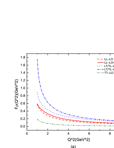
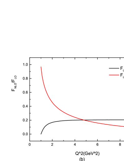
Figure 6: (a) The PQCD predictions for $Q^{2}$ dependence of the $\rho$-meson form factors $F_{j}(Q^{2})(j=LL,LT/TL,TT)$ with different polarizations. (b) The ratio of the NLO contribution over the LO one for the $\rho$ form factors.

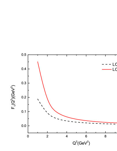
Figure 7: (color online). The PQCD predictions for $Q^{2}$ dependence of electric form factor $F_{1}$.

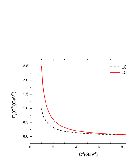
Figure 8: (color online). The PQCD predictions for $Q^{2}$ dependence of magnetic form factor $F_{2}$ .

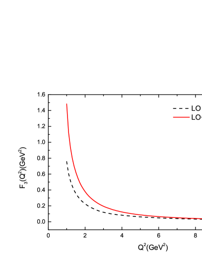
Figure 9: (color online). The PQCD predictions for $Q^{2}$ dependence of quadrupole form factor $F_{3}$.

The results for $\rho$ meson electric $F_{1}(Q^{2})$, magnetic $F_{2}(Q^{2})$ and quadrupole $F_{3}(Q^{2})$ form factors including NLO corrections are shown in Fig. 7, Fig. 8 and Fig. 9 (solid line denotes LO contribution and curve with long dashes is the sum of LO and NLO contribution). Apparently at small $Q^{2}$, our numerical result is not stable. But the value of our prediction is gradually level off at $Q^{2}$ greater than $4GeV^{2}$. The asymptotic behavior of $\rho$ meson form factors, which derived from quark counting and chirality conservation, are $F_{1}(Q^{2})\sim F_{2}(Q^{2})\sim 1/Q^{4}$ and $F_{3}(Q^{2})\sim 1/Q^{6}$. Obviously it can be checked that our numerical result with radiative corrections satisfy this behavior at large $Q^{2}$.

Table 1: The comparisons of our predictions with those from other different approaches for the $\rho$ meson form factors at different values of $Q^{2}$. (Note that value at $Q^{2}=4,5$ for light-front quark-model and $Q^{2}=5$ for three-point QCD sum rules are not given.)

$Q^{2}$(GeV2)	3	4	5
Form factors	$F_{1}$   $F_{2}$   $F_{3}$	$F_{1}$   $F_{2}$   $F_{3}$	$F_{1}$   $F_{2}$   $F_{3}$
Light-front quark-model	0.08   0.41   -0.10	/     /     /	/     /     /
Three-point QCD sum rules	0.07   0.15   0.009	0.05   0.10   0.001	/     /     /
Light cone QCD sum rules	0.08   0.17   -0.15	0.06   0.16   -0.12	0.04   0.12   -0.10
PQCD	0.07   0.30   0.20	0.05   0.20   0.12	0.03   0.15   0.09

The $\rho$ meson form factors have been calculated in the frameworks of different approaches, such as the three-point QCD sum rules, the light cone sum rules, the Light-front quark-model, the lattice QCD, and our PQCD approach. In Table I, we present the values of the electric, magnetic and quadruple form factors predicted by different approaches at different values of $Q^{2}$. At small $Q^{2}$, where the lattice calculation is applicable, our PQCD does not work. So we only selected three values of $Q^{2}$, $Q^{2}=3,4,5$, at intermediate momentum transfer for QCD sum rules and large for our PQCD. We found that our results for electric form factor $F_{1}$ practically identify with the prediction with three-point QCD sum rule and light cone QCD sum rule. Then our prediction for magnetic form factor $F_{2}$ is 2 times larger than QCD sum rules at $Q^{2}=3$, while close to light-front quark-model. But our values are getting closer to the one from QCD sum rules with the increase of $Q^{2}$, at $Q^{2}=3,4$. The value of quadruple form factors $F_{3}$ are much larger than the one for other approaches, which deserve our further consideration. Unfortunately, the PQCD does not work properly at small $Q^{2}$ region, we therefore can not determine magnetic moment of $\rho$ meson in the low-$Q^{2}$ region where both the lattice calculation and the light-front quark model can work well.

IV CONCLUSION

In this paper we studied the $\rho\gamma^{*}\to\rho$ transition process and calculated the next-to-leading-order corrections to the $\rho$ meson electromagnetic form factors in the framework of the PQCD factorization approach. We firstly derive the infrared-finite NLO hard kernel for $\rho$ meson electromagnetic form factors by taking the difference of the quark diagrams and the effective diagrams for the pion wave function, and then calculate the NLO corrections to the form factors $F_{i}(Q^{2})(i=LL,LT,TL)$, and present the expressions of the electric $F_{1}(Q^{2})$, the magnetic $F_{2}(Q^{2})$ and the quadruple $F_{3}(Q^{2})$ form factors of $\rho$ meson in the hard scale. We found that the NLO corrections to $F_{LT,TL}$ are around $30\%$ of the LO contribution in the region $Q^{2}>2GeV^{2}$, where the PQCD approach is applicable. The NLO correction to $F_{LL}(Q^{2})$ is around $20\%$ of the LO one in the region $Q^{2}>3GeV^{2}$. The NLO radiative corrections to the electric, the magnetic, and the quadruple form factors $F_{j}(Q^{2})(j=1,2,3)$ are sizeable in magnitude, and do agree with the results from the QCD sum rules.

V ACKNOWLEDGEMENTS

Many thanks to Shan Cheng for valuable discussions. This work is supported by the National Natural Science Foundation of China under Grants No.11847141 and 11775117, and also by the Practice Innovation Program of Jiangsu Province under Grant No. KYCX18-1184.

References

(1)
H. N. Li, Perturbative QCD factorization of and ,
Phys. Rev. D64, 014019 (2001).
(2)
M. Nagashima and H. N. Li, factorization of exclusive processes, Phys. Rev. D67, 034001 (2003).
(3)
M. Nagashima and H. N. Li, Two parton twist three factorization in perturbative QCD , Eur. Phys. J. C40, 395 (2005).
(4)
S. Cheng, and Z. J. Xiao, Perturbative QCD factorization of ,
Phys. Rev. D90, 076001 (2014).
(5) Y. L. Zhang, S. Cheng, J. Hua, and Z. J. Xiao, Perturbative QCD factorization of ,
Phys. Rev. D93, 036002 (2016).
(6) J. Hua, Y. L. Zhang, and Z. J. Xiao, Next-to-leading order corrections to transition in the factorization ,
Phys. Rev. D99, 016007 (2019).
(7)
H. N. Li, Y. L. Shen, Y. M. Wang, and H. Zou, Next-to-leading-order correction to pion form factor in factorization ,
Phys. Rev. D83, 054029 (2011).
(8)
S. Cheng, Y. Y. Fan, and Z. J. Xiao, NLO twist-3 contribution to the pion electromagnetic form factors in factorization,
Phys. Rev. D89, 054015 (2014).
(9)
Y. L. Zhang, S. Cheng, J. Hua, and Z. J. Xiao, transition form factors in the perturbative QCD factorization approach, Phys. Rev. D92, 094031 (2015).
(10)
J. Hua, S. Cheng, Y. L. Zhang, and Z. J. Xiao, Rho-pion transition form factors in the factorization formulism revisited,
Phys. Rev. D97, 113002 (2018).
(11) V. V. Braguta and A. I. Onishchenko, rho-meson form factors and QCD sum rules,
Phys. Rev. D70, 033001 (2004).
(12) T. M. Aliev and M. Savci, Electromagnetic form factors of the rho meson in light cone QCD sum rules,
Phys. Rev. D70, 094007 (2004).
(13) H. M. Choi and C. R. Ji, Electromagnetic structure of the rho meson in the light front quark model,
Phys. Rev. D70, 053015 (2004).
(14)
W. Andersen and W. Wilcox, Lattice Charge Overlap I. Elastic Limit of Pi and Rho Mesons,
Ann. Phys.(N.Y.)255, 34 (1997).
(15)
P. Ball, V. M. Braun, Y. Koike and K. Tanaka, Higher twist distribution amplitudes of vector mesons in QCD:Formalism and twist 3 distributions, Nucl. Phys. B529, 323 (1998).
(16)
P. Ball and V. M. Braun, Higher twist distribution amplitudes of vector mesons in QCD: Twist 4 distributions and meson mass corrections, Nucl. Phys. B543, 201 (1999).
(17) C. Wang, Q. A. Zhang, Y. Li and C. D. Lu, Charmless Decays in Factorization-Assisted Topological-Amplitude Approach, Eur. Phys. J. C77, 333 (2017).
(18)
S. J. Brodsky, C. R. Ji, A. Pang, and D. G. Robertson, Optimal renormalization scale and scheme for exclusive processes ,
Phys. Rev. D57, 245 (1998).
(19) T. Huang and Q. X. Shen, A Study of the Applicability of Perturbative QCD to the Pion Form-factor,
Z. Phys. C50, 139 (1991).
(20)
H. N. Li and G. Sterman, The Perturbative pion form-factor with Sudakov suppression ,
Nucl. Phys. B381, 129 (1992).
(21)
J. Botts and G. Sterman, Hard Elastic Scattering in QCD: Leading Behavior, Nucl. Phys. B325, 62 (1989).
(22) G. F. Sterman, Summation of Large Corrections to Short Distance Hadronic Cross-Sections , Nucl. Phys. B281, 310 (1987).
(23)
J. h. Yu, B. W. Xiao and B. Q. Ma, Space-like and time-like pion-rho transition form factors in the light-cone formalism,
J.Phys.-G-34, 1845 (2007).
(24)
F. Zuo, Y. Jia and T. Huang, Transition Form Factor in Extended AdS/QCD Models,
Eur. Phys. J. C67, 253 (2010).
(25)
Y. L. Zhang, X. Y. Liu, Y. Y. Fan, S. Cheng, Z. J. Xiao, decays and effects of the next-to-leading order contributions,
Phys. Rev. D90, 014029 (2014).
(26)
W. F. Wang, H. N. Li, Quasi-two-body decays in perturbative QCD approach,
Phys. Lett. B763, 29 (2016).
(27) Z. Rui, W. F. Wang , S-wave K contributions to the hadronic charmonium B decays in the perturbative QCD approach,
Phys. Rev. D97, 033006 (2018).
(28)
Y. Li, A. J. Ma, W. F. Wang, Z. J. Xiao, Quasi-two-body decays
in the perturbative QCD approach, Phys. Rev. D96,036014(2017).
(29)
A. J. Ma, Y. Li, W. F. Wang, Z. J. Xiao, The quasi-two-body decays in the perturbative QCD , Nucl. Phys. B923 , 54 (2017).
(30)
Q. Qin, Z. T. Zou, X. Yu, H. L. Li and C. D. L, Perturbative QCD study of decays to a pseudoscalar
meson and a tensor meson, Phys. Lett. B732, 36 (2014).
(31)
C. D. L, W. Wang, Y. Xing and Q. A. Zhang, Perturbative QCD analysis of exclusive processes
and , Phys. Rev. D97, 114016 (2018).
(32)
J.C.Collins, What exactly is a parton density? , Acta. Phys. Polon. B 34, 3103 (2003).
(33)
J.P.Ma, Q. Wang, Transverse momentum dependent factorization for radiative leptonic decay of B-meson, J. High Energy Phys. 0601, 067 (2006).
(34) T. D. Lee and M. Nauenberg, Degenerate Systems and Mass Singularities, Phys. Rev.133, B1549 (1964).
(35)
T. Kinoshita, Mass singularities of Feynman amplitudes, J. Math. Phys.3, 650 (1962).
(36)
Y. L. Zhang, S. Cheng, J. Hua, and Z. J. Xiao, Perturbative QCD factorization of ,
Phys. Rev. D93, 036002 (2016).
(37)
S. Catani and L. Trentadue, Resummation of the QCD Perturbative Series for Hard Processes, Nucl. Phys. B327, 323 (1989).
(38) H. N. Li, Resummation in hard QCD processes, Phys. Rev. D55, 105 (1997).
(39)
Z. T. Wei and M. Z. Yang, Phenomenological study of Sudakov effects in the pion form-factor,
Phys. Rev. D67, 094013 (2003).
(40)
H. N. Li, Unification of the and threshold resummations, Phys. Lett. B454 , 328 (1999).
(41)
T. Kurimoto, H. N. Li and A. I. Sanda, Leading power contributions to B —¿ pi, rho transition form-factors,
Phys. Rev. D65, 014007 (2002).
(42)
H. N. Li, Y. L. Shen, Y. M. Wang and H. Zou, Next-to-leading-order correction to pion form factor in factorization,
Phys. Rev. D83, 054029 (2011).
(43)
H. N. Li,Y. M. Wang, Non-dipolar Wilson links for transverse-momentum-dependent wave functions,
J. High Energy Phys. 1506, 013 (2015).
(44)
H. N. Li, Threshold resummation for exclusive B meson decays ,
Phys. Rev. D66, 094010 (2002).
(45)
P. Ball, Theoretical update of pseudoscalar meson distribution amplitudes of higher twist: The Nonsinglet case,
J. High Energy Phys. 9901, 010 (1999);
P. Ball, V. M. Braun and A. Lenz, Higher-twist distribution amplitudes of the K meson in QCD,
J. High Energy Phys. 0605, 004 (2006);
P. Ball and R. Zwicky, New results on decay formfactors from light-cone sum rules,
Phys. Rev. D71, 014015 (2005).
(46) S. Cheng, Y. L. Zhang, J. Hua, H. N. Li and Z. J. Xiao, Revisiting the factorization theorem for at twist 3 , Phys. Rev. D95, 076005 (2017).
(47)
A. Bharucha, D. M. Straub and R. Zwicky, in the Standard Model from light-cone sum rules,
J. High Energy Phys. 1608, 098 (2016).