Tweedie Gradient Boosting for Extremely Unbalanced Zero-inflated Data

Abstract

Tweedie’s compound Poisson model is a popular method to model insurance claims with probability mass at zero and nonnegative, highly right-skewed distribution. In particular, it is not uncommon to have extremely unbalanced data with excessively large proportion of zero claims, and even traditional Tweedie model may not be satisfactory for fitting the data. In this paper, we propose a boosting-assisted zero-inflated Tweedie model, called EMTboost, that allows zero probability mass to exceed a traditional model. We makes a nonparametric assumption on its Tweedie model component, that unlike a linear model, is able to capture nonlinearities, discontinuities, and complex higher order interactions among predictors. A specialized Expectation-Maximization algorithm is developed that integrates a blockwise coordinate descent strategy and a gradient tree-boosting algorithm to estimate key model parameters. We use extensive simulation and data analysis on synthetic zero-inflated auto-insurance claim data to illustrate our method’s prediction performance.

KEY WORDS: Claim frequency and severity; Gradient boosting; Zero-inflated insurance claims data; EM algorithm.

1.   INTRODUCTION

Setting premium for policyholders is one of the most important problems in insurance business, and it is crucial to predict the size of actual but unforeseeable claims. For typical portfolios in property and casualty insurance business, the policy claim for a covered risk usually has a highly right-skewed continuous distribution for positive claims, while having a probability mass at zero when a claim does not occur. This phenomenon poses unique challenges for data analysis as the data cannot be transformed to normality by power transformation and special treatment on zero claims is often required. In particular, Jørgensen and Paes De Souza (1994) and Smyth and Jørgensen (2002) used generalized linear models (GLM; Nelder and Wedderburn, 1972) with a Tweedie distributed outcome, assuming Possion arrival of claims and Gamma distributed amount for individual claims, to simultanuously model frequency and severity of insurance claims. Although Tweedie GLM has been widely used in actuarial studies (e.g., Mildenhall, 1999; Murphy et al., 2000; Sandri and Zuccolotto, 2008), its structure of the logarithmic mean is restricted to a linear form, which can be too rigid for some applications. Zhang (2011) modeled the nonlinearity by adding splines to capture nonlinearity in claim data, and generalized additive models (GAM; Hastie and Tibshirani, 1990; Wood, 2006) can also model nonlinearity by estimating smooth functions. The structures of these models have to be determined a priori by specifying spline degrees, main effects and interactions to be used in the model fitting. More flexibly, Yang et al. (2017) proposed a nonparametric Tweedie model to identify important predictors and their interactions.

Despite the popularity of the Tweedie model under linear or nonlinear logarithmic mean assumptions, it remains under-studied for problems of modeling extremely unbalanced (zero-inflated) claim data. However, it is well-known that the percentage of zeros in insurance claim data can often be well over 90%, posing challenges even for traditional Tweedie model. In statistics literature, there are two general approaches to handle data sets with excess zeros: the “Hurdle-at-zero” models and the “zero-inflated” models. The Hurdle models (e.g., Cragg, 1971; Mullahy, 1986) use a truncated-at-zero strategy, whose examples include truncated Poisson and truncated negative-binomial models. On the other hand, “zero-inflated” models typically use a mixture model strategy, whose examples include zero-inflated Poisson regression and zero-inflated negative binomial regression (e.g., Lambert, 1992; Hall, 2000; Frees et al., 2016), among many notable others.

In this paper, we aim to tackle the entremely unbalanced insurance data problem with excessive zeros by developing a zero-inflated nonparametric Tweedie compound Poisson model. To our knowledge, no existing work systematically studied the zero-inflated Tweedie model and its computational issues. Under a mixture model framework that subsumes traditional Tweedie model as a special case, we develop an Expectation-Maximization (EM) algorithm that efficiently integrates a blockwise coordinate descent algorithm and a gradient boosting-type algorithm to estimate key parameters. We call our method as EMTboost for brevity.

The EMTboost method assumes a mixture of Tweedie model component and a mass zero component. As one interesting feature, it can simultaneously provide estimation for the zero mass probability as well as the dispersion/power parameters of the Tweedie model component, which are useful information in understanding the zero-inflated nature of claim data under analysis. In addition, we employ boosting techniques to fit the mean of the Tweedie component. This boosting approach is motivated by its proven success for nonparametric regression and classification (Freund and Schapire, 1997; Breiman et al., 1998; Breiman, 1999; Friedman, 2001,2002,2001). By integrating a gradient-boosting algorithm with trees as weak learners, the zero-inflated model can learn nonlinearities, discontinuities and complex higher order interactions of predictors, and potentially reduce modeling bias to produce high predictive performance. Due to the inherent use trees, this approach also naturally handles missing values, outliers and various predictor types.

The rest of the article is organized as follows. Section 2 briefly present the models. The main methodology with implementation details is given in Section 3. We use simulation to show performance of EMTboost in Section 4, and apply it to analyze an auto-insurance claim data in Section 5. Brief concluding remarks are given in Section 6.

2.   ZERO-INFLATED TWEEDIE MODEL

To begin with, we give a brief overview of the Tweedie’s compound Poisson model, followed by the introduction of the zero-inflated Tweedie model. Let $N$ be a Poisson random variable denoted by $\mathrm{Pois}(\lambda)$ with mean $\lambda$, and let $\tilde{Z}_{d}$’s ($d=0,1,\dots,N$) be i.i.d Gamma random variables denoted by $\mathrm{Gamma}(\alpha,\gamma)$ with mean $\alpha\gamma$ and variance $\alpha\gamma^{2}$. Assume $N$ is independent of $\tilde{Z}_{d}$’s. Define a compound Poisson random variable $Z$ by

$$Z=\left\{\begin{array}[]{ll}0&\text{if }N=0,\\ \tilde{Z}_{1}+\tilde{Z}_{2}+\cdots+\tilde{Z}_{N}&\text{if }N=1,2,\dots\end{array}\right..$$ (1)

Then $Z$ is a Poisson sum of independent Gamma random variables. The compound Poisson distribution (Jørgensen and Paes De Souza, 1994; Smyth and Jørgensen, 2002) is closely connected to a special class of exponential dispersion models (Jørgensen, 1987) known as Tweedie models (Tweedie, 1984), whose probability density functions are of the form

$$f_{Z}(z|\theta,\phi)=a(z,\phi)\exp\left\{\frac{z\theta-\kappa(\theta)}{\phi}\right\},$$ (2)

where $a(\cdot)$ and $\kappa(\cdot)$ are given functions, with $\theta\in\mathbb{R}$ and $\phi\in\mathbb{R}^{+}$. For Tweedie models, the mean and variance of $Z$ has the property $\mathrm{\mathbb{E}}(Z)\coloneqq\mu=\dot{\kappa}(\theta),~{}\mathrm{Var}(Z)=\phi\ddot{\kappa}(\theta)$, where $\dot{\kappa}(\theta)$ and $\ddot{\kappa}(\theta)$ are the first and second derivatives of $\kappa(\theta)$, respectively. The power mean-variance relationship is $\mathrm{Var}(Z)=\phi\mu^{\rho}$ for some index parameter $\rho\in(1,2)$, which gives $\theta=\mu^{1-\rho}/(1-\rho)$, $\kappa(\theta)=\mu^{2-\rho}/(2-\rho)$ and $\ddot{\kappa}(\theta)=\mu^{\rho}$. If we re-parameterize the compound Poisson model by

$$\lambda=\frac{1}{\phi}\frac{\mu^{2-\rho}}{2-\rho},~{}~{}\alpha=\frac{2-\rho}{\rho-1},~{}~{}\gamma=\phi(\rho-1)\mu^{\rho-1},$$ (3)

then it will have the form of a Tweedie model $\textrm{Tw}(\mu,\phi,\rho)$ with the probability density function

$$f_{\text{Tw}}(z|\mu,\phi,\rho)\coloneqq a(z,\phi,\rho)\exp\left(\frac{1}{\phi}\left(z\frac{\mu^{1-\rho}}{1-\rho}-\frac{\mu^{2-\rho}}{2-\rho}\right)\right)$$ (4)

where

$$a(z,\phi,\rho)=\left\{\begin{array}[]{ll}1,&\text{if }z=0,\\ \frac{1}{z}\sum_{t=1}^{\infty}W_{t}(z,\phi,\rho)\\ ~{}~{}=\frac{1}{z}\sum_{t=1}^{\infty}\frac{z^{t\alpha}}{(\rho-1)^{t\alpha}(2-\rho)^{t}\Gamma(t\alpha)\phi^{t(1+\alpha)}t!},&\text{if }z>0,\end{array}\right.$$ (5)

with $\alpha=(2-\rho)/(\rho-1)$. When $z>0$, the sum of infinite series $\sum_{t=1}^{\infty}W_{t}$ is an example of Weight’s generalized Bessel function.

With the formulation above, the Tweedie model has positive probability mass at zero with $\mathrm{\mathbb{P}}(Z=0)=\mathrm{\mathbb{P}}(N=0)=\exp(-\lambda)$. Despite its popularity in actuarial studies, Tweedie models do not always give ideal performance in cases when the empirical distribution of claim data (e.g., in auto insurance), is extremely unbalanced and has an excessively high proportion of zero claims, which will be illustrated in the numerical exposition. This motivates us to consider a zero-inflated mixture model that combines a Tweedie distribution with probability $q$ and an exact zero mass with probability $1-q$ :

$$Y=\left\{\begin{array}[]{ll}Z,&\text{with probability }q,\ \text{where\ }Z\sim\text{Tw}(\mu,\phi,\rho),\\ 0,&\text{with probability }1-q.\end{array}\right.$$ (6)

We denote this zero-inflated Tweedie model by $Y\sim\text{ZIF-Tw}(\mu,\phi,\rho,q)$. The probability density function of $Y$ can be written as

$$f_{\text{ZIF-Tw}}(y|\mu,\phi,\rho,q)\coloneqq qf_{\text{Tw}}(y|\mu,\phi,\rho)+(1-q)I\left\{y=0\right\},$$ (7)

so that $\mathbb{P}\left(Y=0\right)=q\exp\left(-\frac{1}{\phi}\frac{\mu^{2-\rho}}{2-\rho}\right)+\left(1-q\right)$ and $\mathbb{E}\left(Y\right)=q\mu$.

3.   METHODOLOGY

Consider a portfolio of polices $\mathbf{D}=\{(y_{i},\bm{\mathrm{x}}_{i},\omega_{i})\}_{i=1}^{n}$ from $n$ independent insurance policy contracts, where for the $i$-th contract, $y_{i}$ is the policy pure premium, $\bm{\mathrm{x}}_{i}$ is a $p$-dimensional vector of explanatory variables that characterize the policyholder and the risk being insured, and $\omega_{i}$ is the policy duration, i.e., the length of time that the policy remains in force. Assume that each policy pure premium $y_{i}$ is an observation from the zero-inflated Tweedie distribution $Y_{i}\sim\text{ZIF-Tw}(\mu_{i},\phi/\omega_{i},\rho,q)$ as defined in (6). For now we assume that the value of $\rho$ is given and in the end of this section we will discuss the estimation of $\rho$. Assume $\mu_{i}$ is determined by a regression function $F:\mathbb{R}^{p}\rightarrow\mathbb{R}$ of $\bm{\mathrm{x}}_{i}$ through the $\log$ link function

$$\log(\mu_{i})=\log\left\{\mathrm{\mathbb{E}}\left(Y_{i}|\bm{\mathrm{x}}_{i}\right)\right\}=F(\bm{\mathrm{x}}_{i}).$$ (8)

Let $\bm{\theta}=\left(F,\phi,q\right)\in\mathcal{F}\times\mathbb{R}^{+}\times\left[0,1\right]$ denote a collection of parameters to be estimated with $\mathcal{F}$ denoting a class of regression functions (based on tree learners). Our goal is to maximize the log-likelihood function of the mixture model

$$\widehat{\bm{\theta}}=\arg\max_{\bm{\theta}\in\mathbf{\Theta}}\log\mathcal{L}\left(\bm{\theta};\mathbf{D}\right).$$ (9)

where

$$\mathcal{L}\left(\bm{\theta};\mathbf{D}\right)\coloneqq\prod_{i=1}^{n}f_{\text{ZIF-Tw}}\left(y_{i}|\exp\left(F(\bm{\mathrm{x}}_{i})\right),\phi/\omega_{i},\rho,q\right)$$ , (10)

but doing so directly is computationally difficult. To efficiently estimate $\bm{\theta}=\left(F,\phi,q\right)$, we propose a gradient-boosting based EM algorithm, referred to as EMTboost henceforth. We first give an outline of the EMTboost algorithm and the details will be discussed further in Section 3.1–3.2. The basic idea is to first construct a proxy $Q\text{-function}$ corresponding to the current iterate by which the target likelihood function (10) is lower bounded (E-step), and then maximize the $Q\text{-function}$ to get the next update (M-step) so that 10 can be driven uphill:

E-Step Construction

We introduce $n$ independent Bernoulli latent variables $\Pi_{1},\ldots,\Pi_{n}$ such that for $i=1,\ldots,n$, $P(\Pi_{i}=1)=q$, and $\Pi_{i}=1$ when $y_{i}$ is sampled from $\text{Tweedie}(\mu_{i},\phi/\omega_{i},\rho)$ and $\Pi_{i}=0$ if $y_{i}$ is from the exact zero point mass. Denote $\bm{\Pi}=(\Pi_{1},\ldots,\Pi_{n})^{\top}$. Assume predictors $\mathbf{x}_{i}$’s are fixed. Given $\Pi_{i}\in\left\{0,1\right\}$ and $\bm{\theta}$, the joint-distribution of the complete model for each observation is

$$f\left(y_{i},\Pi_{i}|\bm{\theta}\right)\coloneqq\left(q\cdot f_{\text{Tw}}\left(y_{i}|\exp\left(F(\bm{\mathrm{x}}_{i})\right),\phi,\omega_{i}\right)\right)^{\Pi_{i}}\left(\left(1-q\right)\cdot I\left\{y_{i}=0\right\}\right)^{1-\Pi_{i}}.$$ (11)

The posterior distribution of each latent variable $\Pi_{i}$ is

$$f\left(\Pi_{i}|y_{i},\bm{\theta}\right)=\frac{f\left(y_{i},\Pi_{i}|\bm{\theta}\right)}{f\left(y_{i},\Pi_{i}|\bm{\theta}\right)+f\left(y_{i},1-\Pi_{i}|\bm{\theta}\right)}.$$ (12)

For the E-step construction, denote $\bm{\theta}^{t}=\left(F^{t},\phi^{t},q^{t}\right)$ the value of $\bm{\theta}$ during $t$-th iteration of the EMTboost algorithm. The $Q\text{-function}$ for each observation is

$$Q_{i}\left(\bm{\theta}|\bm{\theta}^{t}\right) \coloneqq\mathbb{E}_{\Pi_{i}\sim f\left(\Pi_{i}|y_{i},\bm{\theta}^{t}\right)}\left[\log f\left(y_{i},\Pi_{i}|\bm{\theta}\right)\right]$$

$$=f\left(\Pi_{i}=1|y_{i},\bm{\theta}^{t}\right)\log f\left(y_{i},\Pi_{i}=1|\bm{\theta}\right)+f\left(\Pi_{i}=0|y_{i},\bm{\theta}^{t}\right)\log f\left(y_{i},\Pi_{i}=0|\bm{\theta}\right)$$

$$=\delta_{1,i}^{t}(\bm{\theta}^{t})\log\left(q\cdot f_{\text{Tw}}\left(y_{i}|\exp\left(F(\textbf{x}_{i})\right),\phi,\omega_{i}\right)\right)+\delta_{0,i}^{t}(\bm{\theta}^{t})\log\left(1-q\right)I\left\{y_{i}=0\right\},$$ (13)

where

$$\delta_{1,i}^{t} (\bm{\theta}^{t})=f\left(\Pi_{i}=1|y_{i},\bm{\theta}^{t}\right)=\left\{\begin{array}[]{ll}1,&\text{if }y_{i}>0;\\ \frac{q^{t}\exp\left(\frac{\omega_{i}}{\phi^{t}}\left(-\frac{\exp\left(F^{t}\left(\textbf{x}_{i}\right)\left(2-\rho\right)\right)}{2-\rho}\right)\right)}{q^{t}\exp\left(\frac{\omega_{i}}{\phi^{t}}\left(-\frac{\exp\left(F^{t}\left(\textbf{x}_{i}\right)\left(2-\rho\right)\right)}{2-\rho}\right)\right)+\left(1-q^{t}\right)},&\text{if }y_{i}=0,\end{array}\right.$$ (16)

$$\delta_{0,i}^{t} (\bm{\theta}^{t})=f\left(\Pi_{i}=0|y_{i},\bm{\theta}^{t}\right)=1-\delta_{1,i}^{t}(\bm{\theta}^{t})$$ (17)

Given $n$ observations of data $\mathbf{D}=\{(y_{i},\bm{\mathrm{x}}_{i},\omega_{i})\}_{i=1}^{n}$, the $Q\text{-function}$ is

$$Q\left(\bm{\theta}|\bm{\theta}^{t}\right) =\frac{1}{n}\sum_{i=1}^{n}Q_{i}\left(\bm{\theta}|\bm{\theta}^{t}\right)$$

$$=\frac{1}{n}\sum_{i=1}^{n}\delta_{1,i}^{t}(\bm{\theta}^{t})\log\left(q\cdot f_{\text{Tw}}\left(y_{i}|\exp\left(F(\bm{\mathrm{x}}_{i})\right),\phi,\omega_{i}\right)\right)+\delta_{0,i}^{t}(\bm{\theta}^{t})\log\left(\left(1-q\right)\cdot I\left\{y_{i}=0\right\}\right)$$

$$=\frac{1}{n}\sum_{i=1}^{n}\delta_{1,i}^{t}(\bm{\theta}^{t})\log\left\{qa(y_{i},\phi/\omega_{i},\rho)\exp\left[\frac{\omega_{i}}{\phi}\left(y_{i}\frac{\exp\left((1-\rho)F(\bm{\mathrm{x}}_{i})\right)}{1-\rho}-\frac{\exp\left((2-\rho)F(\bm{\mathrm{x}}_{i})\right)}{2-\rho}\right)\right]\right\}$$

$$+\frac{1}{n}\sum_{\{i:y_{i}=0\}}\delta_{0,i}^{t}(\bm{\theta}^{t})\log\left(1-q\right)$$ (18)

M-Step Maximization

Given the $Q\text{-function}$ (18), we update $\bm{\theta}^{t}$ to $\bm{\theta}^{t+1}$ through maximization of (18) by

$$\bm{\theta}^{t+1}=\left(F^{t+1},\phi^{t+1},q^{t+1}\right)\longleftarrow\arg\max_{\bm{\theta}\in\bm{\Theta}}Q\left(\bm{\theta}|\bm{\theta}^{t}\right),$$ (19)

in which $F^{t+1}$, $\phi^{t+1}$ and $q^{t+1}$ are updated successively through blockwise coordinate descent

$$F^{t+1} \longleftarrow\arg\max_{F\in\mathcal{F}}Q\left(F|\left(F^{t},\phi^{t},q^{t}\right)\right)$$ (20)

$$\phi^{t+1} \longleftarrow\arg\max_{\phi\in\mathbb{R}^{+}}Q\left(\phi|\left(F^{t+1},\phi^{t},q^{t}\right)\right)$$ (21)

$$q^{t+1} \longleftarrow\arg\max_{q}Q\left(q|\left(F^{t+1},\phi^{t+1},q^{t}\right)\right)$$ (22)

Specifically, (20) is equivalent to update

$$F^{t+1} \longleftarrow\arg\max_{F\in\mathscr{F}}\sum_{i=1}^{n}\delta_{1,i}^{t}(F^{t},\phi^{t},q^{t})\Psi(y_{i},F(\bm{\mathrm{x}}_{i}),\omega_{i}),$$ (23)

where the risk function $\Psi$ is defined as

$$\Psi(y_{i},F(\bm{\mathrm{x}}_{i}),\omega_{i})=\omega_{i}\left(y_{i}\frac{\exp\left(F\left(\bm{\mathrm{x}}_{i}\right)\left(1-\rho\right)\right)}{1-\rho}-\frac{\exp\left(F\left(\bm{\mathrm{x}}_{i}\right)\left(2-\rho\right)\right)}{2-\rho}\right).$$ (24)

We use a gradient tree-boosted algorithm to compute (23), and its details are deferred to Section 3.1. After updating $F^{t+1}$ we then update $\phi^{t+1}$ in (21) using

$$\phi^{t+1} \longleftarrow\arg\max_{\phi\in\mathbb{R}^{+}}\sum_{i=1}^{n}\delta_{1,i}^{t}(F^{t+1},\phi^{t},q^{t})\Biggl{\{}\log a(y_{i},\phi/\omega_{i},\rho),$$ (25)

$$+\frac{\omega_{i}}{\phi}\left(y_{i}\frac{\exp\left((1-\rho)F^{t+1}(\bm{\mathrm{x}}_{i})\right)}{1-\rho}-\frac{\exp\left((2-\rho)F^{t+1}(\bm{\mathrm{x}}_{i})\right)}{2-\rho}\right)\Biggl{\}}.$$

Conditional on the updated $F^{t+1}$ and $q^{t}$, maximizing the log-likelihood function with respect to $\phi$ in (25) is a univariate optimization problem that can be solved by using a combination of golden section search and successive parabolic interpolation (Brent, 2013).

After updating $F^{t+1}$ and $\phi^{t+1}$, we can use a simple formula to update $q^{t+1}$ for (22)

$$q^{t+1}\longleftarrow\frac{1}{n}\sum_{i=1}^{n}\delta_{1,i}^{t}\left(F^{t+1},\phi^{t+1},q^{t}\right).$$ (26)

We repeat the above E-step and M-step iteratively until convergence. In summary, the complete EMTboost algorithm is shown in Algorithm 1.

1

Input : Dataset $\mathbf{D}=\{(y_{i},\bm{\mathrm{x}}_{i},\omega_{i})\}_{i=1}^{n}$ and the index parameter $\rho$.

Output : Estimates $\widehat{\bm{\theta}}=(\widehat{F},\widehat{\phi},\widehat{q})$.

2

3Initialize $\bm{\theta}^{0}=(F^{0},\phi^{0},\rho^{0})$. Compute the index set $\mathcal{I}=\{i:y_{i}=0\}$ and initialize $\{\delta_{0,i}^{0},\delta_{1,i}^{0}\}_{i\in\mathcal{I}}$ by setting $\delta_{1i}=1,\delta_{0i}=0$ for $i\notin\mathcal{I}$. 

4for $t=0,1,2,\ldots,T$ do

5       E-step: Update $\{\delta_{0,i}^{t},\delta_{1,i}^{t}\}_{i\in\mathcal{I}}$ by (16) and (17).

6      M-step: Update $\bm{\theta}^{t+1}=\left(F^{t+1},\phi^{t+1},q^{t+1}\right)$ by using (23) that calls Algorithm 3, (25) and (26).

$$F^{t+1} \longleftarrow\arg\max_{F\in\mathcal{F}}Q\left(F|\left(F^{t},\phi^{t},q^{t}\right)\right)$$

$$\phi^{t+1} \longleftarrow\arg\max_{\phi\in\mathbb{R}^{+}}Q\left(\phi|\left(F^{t+1},\phi^{t},q^{t}\right)\right)$$

$$q^{t+1} \longleftarrow\arg\max_{q}Q\left(q|\left(F^{t+1},\phi^{t+1},q^{t}\right)\right)$$

7 end for

8Return $\widehat{\bm{\theta}}=(\widehat{F},\widehat{\phi},\widehat{q})=\left(F^{T},\phi^{T},q^{T}\right)$.

Algorithm 1 EMTboost Algorithm

So far we only assume that the value of $\rho$ is known when estimating $\bm{\theta}=\left(F,\phi,q\right)$. Next we give a profile likelihood method to jointly estimate $(\bm{\theta},\rho)=\left(F,\phi,q,\rho\right)$ when $\rho$ is unknown. Following Dunn and Smyth (2005), we pick a sequence of $K$ equally-spaced candidate values $\{\rho_{1},\cdots,\rho_{K}\}$ on the interval $(1,2)$, and for each fixed $\rho_{k}$, $k=1,\ldots,K$, we apply Algorithm 1 to maximize the log-likelihood function (10) with respect to $\bm{\theta}_{\rho_{k}}=\left(F_{\rho_{k}},\phi_{\rho_{k}},q_{\rho_{k}}\right)$, which gives the corresponding estimators $\widehat{\bm{\theta}}_{\rho_{k}}=\left(\widehat{F}_{\rho_{k}},\widehat{\phi}_{\rho_{k}},\widehat{q}_{\rho_{k}}\right)$ and the log-likelihood function $\mathcal{L}\left(\widehat{\bm{\theta}}_{\rho_{k}};\mathbf{D},\rho_{k}\right)$. Then from the sequence $\{\rho_{1},\cdots,\rho_{K}\}$ we choose the optimal $\widehat{\rho}$ as the maximizer of $\mathcal{L}$.

$$\widehat{\rho}=\arg\max_{\rho\in\{\rho_{1},\cdots,\rho_{K}\}}\left\{\mathcal{L}\left(\widehat{\bm{\theta}}_{\rho};\mathbf{D},\rho\right)\right\}.$$ (27)

We then obtain the corresponding estimator $\widehat{\bm{\theta}}_{\widehat{\rho}}=\left(\widehat{F}_{\widehat{\rho}},\widehat{\phi}_{\widehat{\rho}},\widehat{q}_{\widehat{\rho}}\right)$.

1

Input : Dataset $\mathbf{D}=\{(y_{i},\bm{\mathrm{x}}_{i},\omega_{i})\}_{i=1}^{n}$.

Output : Estimates $\widehat{\bm{\theta}}_{\widehat{\rho}}=\left(\widehat{F}_{\widehat{\rho}},\widehat{\phi}_{\widehat{\rho}},\widehat{q}_{\widehat{\rho}}\right)$.

2 Pick a sequence of $K$ equally-spaced candidate values $\{\rho_{1},\cdots,\rho_{K}\}$ on the interval $(1,2)$. for $k=1,\ldots,K$ do

3       Set $\rho=\rho_{k}$.

4      Call Algorithm 1 to compute $\widehat{\bm{\theta}}_{\rho_{k}}=\left(\widehat{F}_{\rho_{k}},\widehat{\phi}_{\rho_{k}},\widehat{q}_{\rho_{k}}\right)$ and the corresponding log-likelihood function $\mathcal{L}\left(\widehat{\bm{\theta}}_{\rho_{k}};\mathbf{D},\rho_{k}\right)$.

5 end for

6Compute the optimal $\widehat{\rho}$

$$\widehat{\rho}={\arg\max}_{\rho\in\{\rho_{1},\cdots,\rho_{K}\}}\left\{\mathcal{L}\left(\widehat{\bm{\theta}}_{\rho};\mathbf{D},\rho\right)\right\}.$$

7Return the final estimator $\widehat{\bm{\theta}}_{\widehat{\rho}}=\left(\widehat{F}_{\widehat{\rho}},\widehat{\phi}_{\widehat{\rho}},\widehat{q}_{\widehat{\rho}}\right)$.

Algorithm 2 Profile Likelihood for EMTboost

3.1.   Estimating $F\left(\cdot\right)$ via Tree-based Gradient Boosting

To minimize the weighted sum of the risk function (24), we employ the tree-based gradient boosting algorithm to recover the predictor function $F\left(\cdot\right)$ :

$$\widetilde{F}(\cdot)=\arg\min_{F(\cdot)\in\mathcal{F}}\sum_{i=1}^{n}\delta_{1,i}\Psi(y_{i},F(\bm{\mathrm{x}}_{i}),\omega_{i}),$$ (28)

Note that the objective function does not depend on $\phi$. To solve the gradient-tree boosting, each candidate function $F\in\mathcal{F}$ is assumed to be an ensemble of $L$-terminal nodes regression trees, as base learners:

$$F(\mathbf{x}) =F^{[0]}+\sum_{m=1}^{M}\beta^{[m]}h\left(\bm{\mathrm{x}};\bm{\xi}^{[m]}\right),$$ (29)

$$=F^{[0]}+\sum_{m=1}^{M}\beta^{[m]}\left\{\sum_{l=1}^{L}u_{l}^{[m]}I(\bm{\mathrm{x}}\in R_{l}^{[m]})\right\}$$ (30)

where $F^{[0]}$ is a constant scalar, $\beta^{[m]}$ is the expansion coefficient and $h(\bm{\mathrm{x}};\bm{\xi}^{[m]})$ is the $m$-th base learner, characterized by the parameter $\bm{\xi}^{[m]}=\{R_{l}^{[m]},u_{l}^{[m]}\}_{l=1}^{L}$ , with $R_{l}^{[m]}$ being the disjoint regions representing the terminal nodes of the tree, and constants $u_{l}^{[m]}$ being the values assigned to each region.

The constant $\widehat{F}^{[0]}$ is chosen as the $1$-terminal tree that minimizes the negative log-likelihood. A forward stagewise algorithm (Friedman, 2001) builds up the components $\beta^{[m]}h\left(\bm{\mathrm{x}};\bm{\xi}^{[m]}\right)$ sequentially through a gradient-descent-like approach with $m=1,2,\dots,M$. At iteration stage $m$, suppose that the current estimation for $\widetilde{F}\left(\cdot\right)$ is $\widehat{F}^{[m-1]}\left(\cdot\right)$. To update from $\widehat{F}^{[m-1]}\left(\cdot\right)$ to $\widehat{F}^{[m]}\left(\cdot\right)$, the gradient-tree boosting method fits the $m$-th regression tree $h\left(\bm{\mathrm{x}};\bm{\xi}^{[m]}\right)$ to the negative gradient vector by least-squares function minimization:

$$\widehat{\bm{\xi}}^{\left[m\right]}=\arg\min_{\bm{\xi}^{\left[m\right]}}\sum_{i=1}^{n}\left[g_{i}^{\left[m\right]}-h\left(\bm{\mathrm{x}}_{i};\bm{\xi}^{[m]}\right)\right]^{2},$$ (31)

where $\left(g_{1}^{\left[m\right]},\cdots,g_{n}^{\left[m\right]}\right)^{\top}$is the current negative gradient vector of $\Psi$ with respect to (w.r.t.) $\widehat{F}^{\left[m-1\right]}$:

$$g_{i}^{\left[m\right]}=-\frac{\partial\Psi\left(y_{i},F\left(\bm{\mathrm{x}}_{i}\right),\omega_{i}\right)}{\partial F\left(\bm{\mathrm{x}}_{i}\right)}\bigg{|}_{F\left(\bm{\mathrm{x}}_{i}\right)=\widehat{F}^{\left[m-1\right]}\left(\bm{\mathrm{x}}_{i}\right)}.$$ (32)

When fitting this regression trees, first use a fast top-down “best-fit” algorithm with a least-squares splitting criterion (Friedman et al., 2000) to find the splitting variables and the corresponding splitting locations that determine the terminal regions $\{\widehat{R}_{l}^{[m]}\}_{l=1}^{L}$, then estimate the terminal-node values $\{\hat{u}_{l}^{[m]}\}_{l=1}^{L}$ . This fitted regression tree $h(\bm{\mathrm{x}};\{\hat{u}_{l}^{[m]},\widehat{R}_{l}^{[m]}\}_{l=1}^{L})$ can be viewed as a tree-constrained approximation of the unconstrained negative gradient. Due to the disjoint nature of the regions produced by regression trees, finding the expansion coefficient $\beta^{[m]}$ can be reduced to solving $L$ optimal constants $\eta_{l}^{[m]}$ within each region $\hat{R}_{l}^{[m]}$. And the estimation of $\tilde{F}$ for the next stage becomes

$$\widehat{F}^{[m]}=\widehat{F}^{[m-1]}+\nu\sum_{l=1}^{L}\hat{\eta}_{l}^{[m]}I(\bm{\mathrm{x}}\in\widehat{R}_{l}^{[m]}),$$ (33)

where $0\leq\nu\leq 1$ is the shrinkage factor that controls the update step size. A small $\nu$ imposes more shrinkage, while $\nu=1$ gives complete negative gradient steps. Friedman (2001) has found that the shrinkage factor reduces overfitting and improve the predictive accuracy. The complete algorithm is shown in Algorithm 3.

1

Input : Dataset $\mathbf{D}=\{(y_{i},\bm{\mathrm{x}}_{i},\omega_{i})\}_{i=1}^{n}$ and the index parameter $\rho$.

Output : Estimates $\widehat{F}$.

2

3Initialize $\widehat{F}^{[0]}=\log\left(\frac{\sum_{i=1}^{n}\omega_{i}y_{i}}{\sum_{i=1}^{n}\omega_{i}}\right)$. 

4for $m=0,1,2,\ldots,M$ do

5       Compute the negative gradient vector $(g_{1}^{[m]},\ldots,g_{n}^{[m]})^{\top}$

$$g_{i}^{[m]}=\omega_{i}\left\{-y_{i}\exp\left[(1-\rho)\widehat{F}^{[m-1]}(\bm{\mathrm{x}}_{i})\right]+\exp\left[(2-\rho)\widehat{F}^{[m-1]}(\bm{\mathrm{x}}_{i})\right]\right\},i=1,\ldots,n.$$

6      Fit the negative gradient vector to $(\bm{\mathrm{x}}_{1},\ldots,\bm{\mathrm{x}}_{n})^{\top}$ by an $L$-terminal node regression tree, giving the partition $\{\widehat{R}_{l}^{[m]}\}_{l=1}^{L}$.

7      Compute the optimal terminal node predictions $\eta_{l}^{[m]}$ for each region $\widehat{R}_{l}^{[m]}$, $l=1,2,\ldots,L$

$$\hat{\eta}_{l}^{[m]}=\log\left(\frac{\sum_{i:\bm{\mathrm{x}}_{i}\in\widehat{R}_{l}^{[m]}}\omega_{i}y_{i}\exp\left[(1-\rho)\widehat{F}^{[m-1]}(\bm{\mathrm{x}}_{i})\right]}{\sum_{i:\bm{\mathrm{x}}_{i}\in\widehat{R}_{l}^{[m]}}\omega_{i}y_{i}\exp\left[(2-\rho)\widehat{F}^{[m-1]}(\bm{\mathrm{x}}_{i})\right]}\right)$$

8      Update $\widehat{F}^{[m]}$ for each region $\widehat{R}_{l}^{[m]}$ by (33).

9 end for

10Return $\widehat{F}=\widehat{F}^{[M]}$.

Algorithm 3 TDboost Algorithm

3.2.   Implementation details

Next we give a data-driven method to find initial values for parameter estimation. The idea is that we approximately view the latent variables as $\Pi_{i}\approx I\{y_{i}\neq 0\}$. That is, we treat all zeros as if they are all from the exact zero mass portion, which can be reasonable for extremely unbalanced zero-inflated data. If the latent variables were known, it is straightforward to find the MLE solution of a constant mean model:

$$\bm{\theta}^{0}=\arg\max_{\bm{\theta}\in\bm{\Theta}}\log\mathcal{L}\left(\bm{\theta};\mathbf{D},\widetilde{\bm{\Pi}}\right),$$ (34)

where $\bm{\Theta}=\mathcal{C}\times\mathbb{R}^{+}\times\left[0,1\right]$ , $\mathcal{C}=\left\{F\equiv\eta\,|\,\eta\in\mathbb{R}\right\}$, and $\eta$ is a constant scalar. We then find initial values successively as follows:

Initialize $F^{0}$ by

$$F^{0}= \arg\min_{\eta\in\mathbb{R}}\sum_{i=1}^{n}I\{y_{i}\neq 0\}\cdot\Psi(y_{i},\eta,\omega_{i})$$

$$= \log\left[\frac{\sum_{i=1}^{n}I\{y_{i}\neq 0\}\cdot y_{i}\cdot\omega_{i}}{\sum_{i=1}^{n}I\{y_{i}\neq 0\}\cdot\omega_{i}}\right].$$ (35)

Initialize $\phi^{0}$ by

$$\phi^{0}=\arg\min_{\phi\in\mathbb{R}^{+}}\sum_{i=1}^{n}I\{y_{i}\neq 0\}\left(\log a(y_{i},\phi/\omega_{i},\rho)+\frac{\omega_{i}}{\phi}(y_{i}\frac{\exp\left(F^{0}\left(1-\rho\right)\right)}{1-\rho}-\frac{\exp\left(F^{0}\left(2-\rho\right)\right)}{2-\rho})\right),$$ (36)

Initialize $q^{0}$ by

$$q^{0}=\frac{1}{n}\sum_{i=1}^{n}I\{y_{i}\neq 0\}.$$ (37)

Given $\bm{\theta}^{0}$ obtained above, we can then initialize $(\delta_{1,i},\delta_{0,i})$ by equation (16) and (17), giving $\left(\delta_{0,i}^{0},\delta_{1,i}^{0}\right)$.

As a last note, when implementing EMTboost algorithm, for more stable computation, we may want to avoid that the probability $q$ converges to $1$ (or 0). In such case, we can add a regularization term $r\log(1-q)$ on $q$ so that each M-step in Q-function (18) becomes

$$\mathcal{P}Q\left(\bm{\theta}|\mathbb{\bm{\theta}}^{t}\right)=Q\left(\bm{\theta}|\mathbb{\bm{\theta}}^{t}\right)+\underbrace{r\log\left(1-q\right)}_{\text{regularization term}},$$ (38)

where $r\in\mathbb{R}^{+}$ is a non-negative regularization parameter. Apparently, when maximizing the penalized log-likelihood function (38), larger $q$ will be penalized more. We establish the EM algorithm similar as before, and only need to modify the Maximization step of (26) w.r.t. $q$:

$$q_{\mathcal{P}}^{t+1}=\frac{\frac{1}{n}\sum_{i=1}^{n}\delta_{1,i}^{t}}{r+1},$$ (39)

pulling the original update $q^{t+1}=\frac{1}{n}\sum_{i=1}^{n}\delta_{1,i}^{t}$ towards $0$ by fraction $r+1$. Alternatively, if in some cases, we want to avoid that the EMTboost model degrades to an exact zero mass, the regularization term can be chosen as $r\log\left(1-|1-2q|\right)$. The updating step with respect to $q$ becomes a soft thresholding update with the threshold $r$:

$$q_{\mathcal{P}^{\prime}}^{t+1}=\frac{1}{2}-\frac{\mathcal{S}_{r}\left(1-\frac{2}{n}\sum_{i=1}^{n}\delta_{1,i}^{t}\right)}{2(r+1)}$$ (40)

where $\mathcal{S}_{r}(\cdot)$ is the soft thresholding function with $\mathcal{S}_{r}(x)=\text{sign}(x)(|x|-r)_{+}$. We apply these penalized EMTboost methods to the real data application in Appendix C.1.

4.   SIMULATION STUDIES

In this section, we compare the EMTboost model (Section 3) with a regular Tweedie boosting model (that is $q\equiv 1$; TDboost) and the Gradient Tree-Boosted Tobit model (Grabit; Sigrist and Hirnschall, 2017) in terms of the function estimation performance. The Grabit model extends the Tobit model (Tobin, 1958) using gradient-tree boosting algorithm. We here present two simulation studies in which zero-inflated data are generated from zero-inflated Tweedie model (Case 1 in Section 4.2) and zero-inflated Tobit model (Case 2 in Section 4.3). An additional simulation result (Case 3) in which data are generated from a Tweedie model is put in Appendix B.

Fitting Grabit, TDboost and EMTboost models to these data sets, we get the final predictor function $\hat{F}\left(\cdot\right)$ and parameter estimators. Then we make a prediction about the pure premium by applying the predictor functions on an independent held-out testing set to find estimated expectation: $\widehat{\mu}(\textbf{x})=\mathbb{E}\left(y|\textbf{x}\right)$. For the three competing models, the predicted pure premium is given by equations

$$\widehat{\mu}^{\text{Grabit}}(\textbf{x}) =\varphi\left(-\hat{F}_{\text{Grabit}}(\textbf{x})\right)+\hat{F}_{\text{Grabit}}(\textbf{x})\left(1-\Phi\left(-\hat{F}_{\text{Grabit}}(\textbf{x})\right)\right),$$ (41)

$$\widehat{\mu}^{\text{TDboost}}(\textbf{x}) =\exp(\hat{F}_{\text{TDboost}}(\textbf{x})),$$ (42)

$$\widehat{\mu}^{\text{EMTboost}}(\textbf{x}) =(1-\widehat{q}_{\text{EMTboost}})\exp\left(\hat{F}_{\text{EMTboost}}(\textbf{x})\right),$$ (43)

where $\varphi\left(\cdot\right)$ is the probability density function of the standard normal distribution and $\Phi(\cdot)$ is its cumulative distribution function. The predicted pure premium of the Grabit model is derived in detail in Appendix A. As the true model is known in simulation settings, we can campare the difference between the predicted premiums and the expected true losses. For the zero-inflated Tobit model in case 2, the expected true loss of this model is given by $\mathbb{E}_{\text{ZIF-Tobit}}\left[y|F\left(\textbf{x}\right)\right]=q\left[\varphi\left(-F\left(\textbf{x}\right)\right)+F\left(\textbf{x}\right)\left(1-\Phi\left(-F\left(\textbf{x}\right)\right)\right)\right]$, with $q$ being the probability that response $y$ comes from the Tobit model and $F\left(\textbf{x}\right)$ the true target funtion.

4.1.   Measurement of Prediction Accuracy

Given a portfolio of policies $\mathbf{D}=\{(y_{i},\bm{\mathrm{x_{i}}},\omega_{i})\}_{i=1}^{n}$, $y_{i}$ is the claim cost for the $i$-th policy and $\hat{y}_{i}$ is denoted as the predicted claim cost. We consider the following three measurements of prediction accuracy of $\left\{\hat{y}_{i}\right\}_{i=1}^{n}$.

Gini Index ($\text{Gini}^{a}$)   

Gini index is a well-accepted tool to evaluate the performance of predictions. There exists many variants of Gini index and one variant we use is denoted by $\text{Gini}^{a}$ (Ye et al., 2018): for a sequence of numbers $\{s_{1},\cdots,s_{n}\}$, let $R(s_{i})\in\{1,\cdots,n\}$ be the rank of $s_{i}$ in the sequence in an increasing order. To break the ties when calculating the order, we use the LAST tie-breaking method, i.e., we set $R(s_{i})>R(s_{j})$ if $s_{i}=s_{j},~{}i<j$. Then the normalized Gini index is referred to as:

$$\text{Gini}^{a}=\frac{\frac{\sum_{i=1}^{n}y_{i}R(\hat{y}_{i})}{\sum_{i=1}^{n}y_{i}}-\sum_{i=1}^{n}\frac{n-i+1}{n}}{\frac{\sum_{i=1}^{n}y_{i}R(y_{i})}{\sum_{i=1}^{n}y_{i}}-\sum_{i=1}^{n}\frac{n-i+1}{n}}.$$ (44)

Note that this criterion only depends on the rank of the predictions and larger $\text{Gini}^{a}$ index means better prediction performance.

Gini Index ($\text{Gini}^{b}$)   

We exploit an popular alternative–the ordered Lorentz curve and the associated Gini index (denoted by $\text{Gini}^{b}$; Frees et al., 2011, 2014) to capture the discrepancy between the expected premium $P(\textbf{x})=\widehat{\mu}(\textbf{x})$ and the true losses $y$. We successively specify the prediction from each model as the base premium and use predictions from the remaining models as the competing premium to compute the $\text{Gini}^{b}$ indices. Let $B(\textbf{x})$ be the “base premium” and $P(\textbf{x})$ be the “competing premium”. In the ordered Lorentz curve, the distribution of losses and the distribution of premiums are sorted based on the relative premium $R(\textbf{x})=P(\textbf{x})/B(\textbf{x})$. The ordered premium distribution is

$$\hat{D}_{P}(s)=\frac{\sum_{i=1}^{n}B(\textbf{x}_{i})I\left\{R(\textbf{x}_{i})\leq s\right\}}{\sum_{i=1}^{n}B(\textbf{x}_{i})},$$ (45)

and the ordered loss distribution is

$$\hat{D}_{L}(s)=\frac{\sum_{i=1}^{n}y_{i}I\left\{R(\textbf{x}_{i})\leq s\right\}}{\sum_{i=1}^{n}y_{i}}.$$ (46)

Then the ordered Lorentz curve is the graph of $\left(\hat{D}_{P}(s),\hat{D}_{L}(s)\right)$. Twice the area between the ordered Lorentz curve and the line of equality measures the discrepancy between the premium and loss distributions, and is defined as the $\text{Gini}^{b}$ index.

Mean Absolute Deviation (MAD)   

Mean Absolute Deviation with respect to the true losses $\left\{y_{i}\right\}_{i=1}^{n}$ is defined as $\frac{1}{n}\sum_{i=1}^{n}|y_{i}-\hat{y}_{i}|.$ In the following simulation studies, we can directly compute the mean absolute deviation between the predicted losses $\left\{\hat{y}_{i}\right\}_{i=1}^{n}$ and the expected true losses $\left\{\mathbb{E}\left[y_{i}|\textbf{x}_{i}\right]\right\}_{i=1}^{n}$ to obtain $\frac{1}{n}\sum_{i=1}^{n}|\mathbb{E}\left[y_{i}|\textbf{x}_{i}\right]-\hat{y}_{i}|$, while in the real data study, we can only compute the MAD against true losses $\left\{y_{i}\right\}_{i=1}^{n}$.

4.2.   Case 1

In this simulation case, we generate data from the zero-inflated Tweedie models with two different target functions: one with two interactions and the other generated from Friedman (2001)’s “random function generator” (RFG) model. We fit the training data using Grabit, TDboost, and EMTboost. In all numerical studies, five-fold cross-validation is adopted to select the optimal ensemble size $M$ and regression tree size $L$, while the shrinkage factor $\nu$ is set as 0.001.

4.2.1 Two Interactions Function (Case 1.1)

In this simulation study, we demonstrate the performance of EMTboost to recover the mixed data distribution that involves exact zero mass, and the robustness of our model in terms of premium prediction accuracy when the index parameter $\rho$ is misspecified. We consider the true target function with two hills and two valleys:

$$F(x_{1},x_{2})=e^{-5(1-x_{1})^{2}+x_{2}^{2}}+e^{-5x_{1}^{2}+(1-x_{2})^{2}},$$ (47)

which corresponds to a common scenario where the effect of one variable changes depending on the effect of the other. The response $Y$ follows a zero-inflated Tweedie distribution $\text{ZIF-Tw}(\mu,\phi,\rho,q)$ with Tweedie portion probability $q$:

$$Y\sim\left\{\begin{array}[]{ll}Z,&\text{with probability }q,\ \text{Z$\sim$Tw}(\mu,\phi,\rho),\\ 0,&\text{with probability }1-q,\end{array}\right.$$ (50)

where

$$\mu=\exp(F(x_{1},x_{2}))~{},x_{1},x_{2}\text{$\overset{\text{ind}.}{\sim}$}\text{Unif}(0,1),$$

with $\phi=1$, $\rho=1.5$ and $q$ chosen from a decreasing sequence of values: $q\in\{1$, $0.85$, $0.75$, $0.50$, $0.25$, $0.10\}$.

We generate $n=500$ observations $\{\textbf{x}_{i},y_{i}\}_{i=1}^{n}$ for training and $n^{\prime}=1200$ for testing, and fit the training data using Grabit, TDboost and EMTboost models. The true target functions are known, and we use MAD (against expected true premium) and $\text{Gini}^{a}$ index as performance criteria.

When fitting EMTboost, we design three scenarios to illurstrate the robustness of our method w.r.t. $\rho$. In the first scenario, set $\rho=1.5$, which is the true value. In the second scenario, set $\rho=1.7$, which is misspecified. In the last scenario, we use the profile likelihood method to estimate $\rho$.

The resulting MADs and $\text{Gini}^{a}$ indices of the three competing models on the held-out testing data are reported in Table 1 and Table 2, which are averaged over $20$ independent replications for each $q$. Boxplots of MADs comparing Grabit, TDboost and EMTboost (with estimated $\rho$) are shown in Figure 1. In all three scenarios, EMTboost outperforms Grabit and TDboost in terms of the ability to recover the expected true premium by giving smallest MADs and largest $\text{Gini}^{a}$ indices, especially when zeros inflate: $q\in\left\{0.5,0.25,0.1\right\}$. The prediction performance of EMTboost when $\rho=1.7$ is not much worse than that when $\rho=1.5$, showing that the choice of $\rho$ has relatively small effect on estimation accuracy.

Table 1: Simulation results for case 1.1 with MADs.

	Competing Models
$q$	TDboost	Grabit	EMTboost
			$\rho=1.5$	$\rho=1.7$	tuned $\rho$
$1.00$	$0.597\,(.013)$	$0.746\,(.029)$	$0.594\,(.016)$	$0.598\,(.012)$	$0.598\,(.015)$
$0.85$	$0.565\,(.015)$	$0.761\,(.032)$	$0.554\,(.017)$	$0.555\,(.017)$	$0.562\,(.016)$
$0.75$	$0.561\,(.018)$	$0.706\,(.026)$	$0.489\,(.010)$	$0.485\,(.011)$	$0.503\,(.010)$
$0.50$	$0.454\,(.024)$	$0.674\,(.044)$	$0.365\,(.012)$	$0.375\,(.014)$	$0.361\,(.012)$
$0.25$	$0.301\,(.013)$	$0.382\,(.019)$	$0.240\,(.010)$	$0.242\,(.011)$	$0.237\,(.010)$
$0.10$	$0.135\,(.005)$	$0.169\,(.009)$	$0.122\,(.004)$	$0.124\,(.004)$	$0.124\,(.004)$

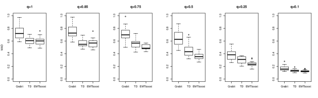
Figure 1: Simulation results for case 1.1: comparing MADs of Grabit, TDboost and EMTboost with decreasing $q$. Boxplots display empirical distributions of MADs based on $20$ independent replications.

Table 2: Simulation results for case 1.1 with $\text{Gini}^{a}$ indices.

	Competing Models
$q$	TDboost	Grabit	EMTboost
			$\rho=1.5$	$\rho=1.7$	tuned $\rho$
$1.00$	$0.480\,(.008)$	$0.449\,(.011)$	$0.481\,(.006)$	$0.481\,(.006)$	$0.481\,(.006)$
$0.85$	$0.393\,(.008)$	$0.354\,(.009)$	$0.397\,(.007)$	$0.397\,(.007)$	$0.397\,(.007)$
$0.75$	$0.343\,(.009)$	$0.300\,(.020)$	$0.363\,(.008)$	$0.365\,(.007)$	$0.361\,(.008)$
$0.50$	$0.242\,(.012)$	$0.186\,(.016)$	$0.289\,(.011)$	$0.288\,(.012)$	$0.292\,(.011)$
$0.25$	$0.172\,(.016)$	$0.116\,(.020)$	$0.219\,(.016)$	$0.215\,(.017)$	$0.217\,(.015)$
$0.10$	$0.085\,(.028)$	$0.107\,(.023)$	$0.137\,(.027)$	$0.122\,(.028)$	$0.136\,(.025)$

4.2.2 Random Function Generator (Case 1.2)

In this case, we compare the performance of the three competing models in various complicated and randomly generated predictor functions. We use the RFG model whose true target function $F$ is randomly generated as a linear expansion of functions $\left\{g_{k}\right\}_{k=1}^{20}$ :

$$F\left(\textbf{x}\right)=\sum_{k=1}^{20}b_{k}g_{k}\left(\textbf{z}_{k}\right).$$ (51)

Here, each coefficient $b_{k}$ is a uniform random variable from Unif$\left[-1,1\right]$. Each $g_{k}\left(\textbf{z}_{k}\right)$ is a function of $\textbf{z}_{k}$, where $\textbf{z}_{k}$ is defined as a $p_{k}$-sized subset of the $p$-dimensional variable x in the form

$$\textbf{z}_{k}=\left\{x_{\psi_{k}\left(j\right)}\right\}_{j=1}^{p_{k}}.$$ (52)

where each $\psi_{k}$ is an independent permutation of the integers $\left\{1,\cdots,p\right\}$. The size $p_{k}$ is randomly selected by $\min\left(\lfloor 2.5+r_{k}\rfloor,p\right)$, where $r_{k}$ is generated from an exponential distribution with mean $2$. Hence, the expected order of interaction presented in each $g_{k}\left(\textbf{z}_{k}\right)$ is between four and five. Each function $g_{k}\left(\textbf{z}_{k}\right)$ is a $p_{k}$-dimensional Gaussian function:

$$g_{k}\left(\textbf{z}_{k}\right)=\exp\left\{-\frac{1}{2}\left(\textbf{z}_{k}-\textbf{u}_{k}\right)^{\text{T}}\textbf{V}_{k}\left(\textbf{z}_{k}-\textbf{u}_{k}\right)\right\},$$ (53)

where each mean vector $\textbf{u}_{k}$ is randomly generated from $\text{N}\left(0,\textbf{I}_{p_{k}}\right)$. The $p_{k}\times p_{k}$ covariance matrix $\textbf{V}_{k}$ is defined by

$$\textbf{V}_{k}=\textbf{U}_{k}\textbf{D}_{k}\textbf{U}_{k}^{\text{T}},$$ (54)

where $\textbf{U}_{k}$ is a random orthonormal matrix, $\textbf{D}_{k}=\text{diag}\left\{d_{k}\left[1\right],\cdots,d_{k}\left[p_{k}\right]\right\}$, and the square root of each diagonal element $\sqrt{d_{k}\left[j\right]}$ is a uniform random variable from $\text{Unif}\left[0.1,2.0\right]$. We generate data $\left\{y_{i},\textbf{x}_{i}\right\}_{i=1}^{n}$ from zero-inflated Tweedie distribution where $\textbf{x}_{i}\sim\text{N}\left(0,\textbf{I}_{p}\right)$, $\mu_{i}=\exp\left\{F\left(\textbf{x}_{i}\right)\right\}$, $i=1,\cdots,n$.

We randomly generate $20$ sets of samples with $\phi=1$ and $\rho=1.5$, each sample having $2000$ observations, $1000$ for training and $1000$ for testing. When fitting EMTboost for each $q\in\left\{1,0.85,0.75,0.5,0.25,0.1\right\}$, the estimates of Tweedie portion probability have mean $\bar{q^{*}}=0.96,0.79,0.71,0.53,0.28,0.13$. Figure 2 shows simulation results comparing the MADs of Grabit, TDboost and EMTboost. We can see, in all the cases, EMTboost outperforms Grabit and becomes very competitive compared to TDboost when $q$ decreases.

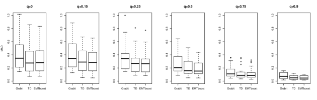
Figure 2: Simulation results for case 1.2: comparing MADs of Grabit, TDboost and EMTboost with decreasing $q$. Boxplots display empirical distributions of the MADs based on $20$ independent replications.

4.3.   Case 2

In this simulation case, we generate data from the zero-inflated Tobit models with two target functions similar to that of case 1. For all three gradient-tree boosting models, five-fold cross-validation is adopted for developing trees. Profile likelihood method is used again.

4.3.1 Two Interactions Function (Case 2.1)

In this simulation study, we compare the performance of three models in terms of MADs. Consider the data generated from the zero-inflated Tobit model where the true target function is given by

$$F(x_{1},x_{2})=2\cos\left(2.4\pi(|x_{1}|^{3}+|x_{2}|^{3})^{0.5}\right).$$ (55)

Conditional on covariates $\textbf{X}=(X_{1},X_{2})$, the latent variable $Y^{*}$ follows a Gaussian distribution:

$$Y^{*}=F(X_{1},X_{2})+\epsilon,~{}X_{k}\text{ i.i.d.}\sim\text{Unif}(-1,1),~{}k=1,2,~{}\epsilon\sim N(0,1).$$

The Tobit response $Y_{\text{Tobit}}$ can be expressed as $Y_{\text{Tobit}}=\max(Y^{*},0)$, and we generate the zero-inflated Tobit data using the Tobit response:

$$Y\sim\begin{cases}Y_{\text{Tobit}},&\text{with probability }q,\\ 0,&\text{with probability }1-q.\end{cases}$$ (56)

where $q$ takes value from the sequence $\left\{1,0.85,0.75,0.5,0.25,0.1\right\}$.

We generate $n=500$ observations for training and $n^{\prime}=4500$ for testing. Figure 3 shows simulation results when comparing MADs of Grabit, TDboost and EMTboost based on $20$ independent replications. We can see from the first boxplot that when $q=1$, zero-inflated Tobit distribution degenerates to a Tobit distribution, and not surprisingly, Grabit outperforms EMTboost in MADs. As $q$ decreases, meaning the proportion of zeros increases, the prediction performance of EMTboost gets improved. When the exact zero mass probability is $1-q=0.9$, the averaged MADs of the three models are $\overline{\text{MAD}}_{\text{Grabit}}=0.0697$, $\overline{\text{MAD}}_{\text{TDboost}}=0.0681$, $\overline{\text{MAD}}_{\text{EMTboost}}=0.0664$, with EMTboost performing the best.

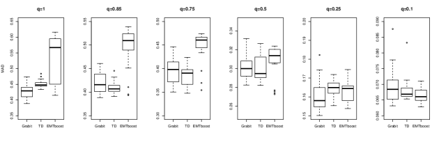
Figure 3: Simulation results for case 2.1: comparing the MADs of Grabit, TDboost and EMTboost with decreasing $q$. Boxplots display empirical distributions of MADs based on $20$ independent replications.

4.3.2 Random Function Generator (Case 2.2)

We again use the RFG model in this simulaiton. The true target function $F$ is randomly generated as given in Section 4.2.2. The latent variable $Y^{*}$ follows

$$Y^{*}=F(\textbf{x}_{i})+\epsilon,~{}\textbf{x}_{i}\sim\text{N}\left(0,\textbf{I}_{p}\right),~{}\epsilon\sim\text{N}(0,1),\;i=1,\cdots,n.$$

We set $Y_{\text{Tobit}}=\max(Y^{*},0)$ and generate the data following the zero-inflated Tobit model (56) with Tobit portion probability $q\in\left\{1,0.85,0.75,0.5,0.25,0.1\right\}$. We randomly generate $20$ sets of sample from the zero-inflated Tobit model for each $q$, and each sample contains $2000$ observations, $1000$ for training and $1000$ for testing. Figure 4 shows MADs of Grabit, TDboost and EMTboost as boxplots. Interestingly, for all the $q$’s, TDboost and EMTboost outperform Grabit even though the true model is a Tobit model. The MAD of EMTboost becomes better when $q$ decreases, and is competitive with that of TDboost when $q=0.1$: the averaged MADs of the three models are $\overline{\text{MAD}}_{\text{Grabit}}=0.0825$, $\overline{\text{MAD}}_{\text{TDboost}}=0.0565$, $\overline{\text{MAD}}_{\text{EMTboost}}=0.0564$. As for the averaged $\text{Gini}^{a}$ indices, EMTboost performs the best when $q=0.1$: $\overline{\text{Gini}^{a}}_{\text{Grabit}}=0.0463$, $\overline{\text{Gini}^{a}}_{\text{TDboost}}=0.0816$, $\overline{\text{Gini}^{a}}_{\text{EMTboost}}=0.1070$.

Figure 4: Simulation results for case 2.2: comparing the MADs of Grabit, TDboost and EMTboost when decreasing $q$. Boxplots display empirical distributions of MADs based on $20$ independent replications.

5.   APPLICATION: AUTOMOBILE CLAIMS

5.1.   Data Set

We consider the auto-insurance claim data set as analyzed in Yip and Yau (2005) and Zhang et al. (2005). The data set contains 10,296 driver vehicle records, each including an individual driver’s total claim amount ($z_{i}$) and 17 characteristics $\textbf{x}_{i}=(x_{i,1},\cdots,x_{i,17})$ for the driver and insured vehicle. We want to predict the expected pure premium based on $\textbf{x}_{i}$. The description statistics of the data are provided in Yang et al. (2017). Approximately $61.1\%$ of policyholders had no claims, and $29.6\%$ of the policyholders had a positive claim amount up to $\$10,000$. Only $9.3\%$ of the policy-holders had a high claim amount above $\$10,000$, but the sum of their claim amount made up to $64\%$ of the overall sum. We use this original data set to synthesize the often more realistic scenarios with extremely unbalanced zero-inflated data sets.

Specifically, we randomly under-sample (without replacement) from the nonzero-claim data with certain fraction $\lambda$ to increase the percentage of the zero-claim data. For example, if we set the under-sampling fraction as $\lambda=0.15$, then the percentage of the non-claim policyholders will become approximately $61.1/(61.1+38.9\lambda)=91.28\%$. We choose a decreasing sequence of under-sampling fractions $\lambda\in\{1,0.75,0.5,0.25,0.15,0.1\}$. For each $\lambda$, we randomly under-sample the positive-loss data without replacement and combine these nonzero-loss data with the zero-loss data to generate a new data set. Then we separate this new data set into two sets uniformly for training and testing . The corresponding percentages of zero-loss data among the new data set w.r.t. different $\lambda$ are presented in Table 3. The Grabit, TDboost and EMTboost models are fitted on the training set and their estimators are obtained with five-fold cross-validation.

Table 3: Real - Zero percentage w.r.t. $\lambda$.

$\lambda$	$1$	$0.75$	$0.50$	$0.25$	$0.15$	$0.10$	$0.05$
Zero Percentage	$61.1\%$	$67.7\%$	$75.9\%$	$86.3\%$	$91.3\%$	$94.0\%$	$96.9\%$

5.2.   Performance Comparison

To compare the performance of Grabit, TDboost and EMTboost models, we predict the pure premium $P(\textbf{x})$ by applying each model on the held-out testing set. Since the losses are highly right-skewed, we use the orderd Lorentz curve and the associated $\text{Gini}^{b}$ index described in Section 4.1 to capture the discrepancy between the expected premiums and true losses.

The entire procedure of under-sampling, data separating and $\text{Gini}^{b}$ index computation are repeated 20 times for each $\lambda$. A sequence of matrices of the averaged $\text{Gini}^{b}$ indices and standard errors w.r.t. each under-sampling fraction $\lambda$ are presented in Table 4. We then follow the “minimax” strategy (Frees et al., 2014) to pick the “best” base premium model that is least vulnerable to the competing premium models. For example, when $\lambda=0.15$, the maximal $\text{Gini}^{b}$ index is $40.381$ when using $B(\textbf{x})=\widehat{\mu}^{\text{Grabit}}(\textbf{x})$ as the base premium, $36.735$ when $B(\textbf{x})=\widehat{\mu}^{\text{TDboost}}(\textbf{x})$ , and $-22.674$ when $B(\textbf{x})=\widehat{\mu}^{\text{EMTboost}}(\textbf{x})$. Therefore, EMTboost has the smallest maximum $\text{Gini}^{b}$ index at $-22.674$, hence having the best performance. Figure 5 also shows that when Grabit (or TDboost) is selected as the base premium, EMTboost represents the most favorable choice.

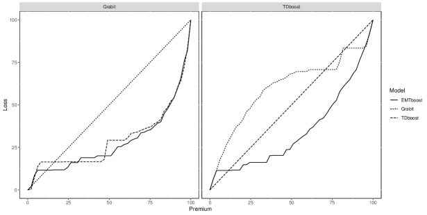
Figure 5: The ordered Lorentz curves for the synthetic data on a single replication when $\lambda=0.15$. Grabit (or TDboost) is set as the base premium and the EMTboost is the competing premium. The ordered Lorentz curve of EMTboost is below the line of equality when choosing Grabit or TDboost as the base premium.

After computing the $\text{Gini}^{b}$ index matrix and using the “minimax” strategy to choose the best candidate model, we count the frequency, out of 20 replications, of each model chosen as the best model and record the ratio of their frequencies. The results w.r.t each $\lambda$ are demenstrated in Figure 6. From Table 4 and Figure 6, we find that when $\lambda$ decreases, the performance of EMTboost gradually outperforms that of TDboost in terms of averaged $\text{Gini}^{b}$ indices and the corresponding model-selection ratios. In particular, TDboost outperforms EMTboost when $\lambda=1,0.75,0.5$, and EMTboost outperforms TDboost when $\lambda=0.25,0.15,0.1,0.05.$ When $\lambda=0.25,0.15,0.1$, EMTboost has the largest model-selection ratio among the three.

Table 4: Grabit, TDboost and EMTboost $\text{Gini}^{b}$ indices. The “best” base premium models are emphasized based on the matrices of averaged $\text{Gini}^{b}$ indices.

	Competing Premium
Base Premium	Grabit	TDboost	EMTboost
	$\lambda=1$
Grabit	$0$	$11.459\,(0.417)$	$11.402\,(0.386)$
TDboost	$\bm{6.638}\,(0.409)$	$0$	$0.377\,(0.355)$
EMTboost	$7.103\,(0.357)$	$2.773\,(0.414)$	$0$
	$\lambda=0.75$
Grabit	$0$	$14.955\,(0.413)$	$15.162\,(0.435)$
TDboost	$\bm{5.466}\,(0.425)$	$0$	$1.848\,(0.504)$
EMTboost	$6.152\,(0.385)$	$2.622\,(0.560)$	$0$
	$\lambda=0.50$
Grabit	$0$	$25.047\,(1.539)$	$25.621\,(1.492)$
TDboost	$3.516\,(0.963)$	$0$	$\bm{4.056}\,(0.651)$
EMTboost	$5.702\,(0.698)$	$2.525\,(0.501)$	$0$
	$\lambda=0.25$
Grabit	$0$	$51.502\,(1.062)$	$51.581\,(1.005)$
TDboost	$-18.248\,(2.445)$	$0$	$20.035\,(2.414)$
EMTboost	$1.283\,(2.593)$	$\bm{3.929}\,(2.544)$	$0$
	$\lambda=0.15$
Grabit	$0$	$37.290\,(2.505)$	$40.381\,(1.822)$
TDboost	$-23.569\,(2.607)$	$0$	$36.735\,(3.188)$
EMTboost	$\bm{-22.674}\,(1.975)$	$-22.926\,(2.604)$	$0$
	$\lambda=0.10$
Grabit	$0$	$-1.189\,(5.828)$	$16.721\,(5.120)$
TDboost	$14.581\,(6.587)$	$0$	$35.298\,(3.026)$
EMTboost	$\bm{-2.742}\,(4.884)$	$-20.080\,(3.572)$	$0$
	$\lambda=0.05$
Grabit	$0$	$-16.851\,(2.662)$	$\bm{-8.652}\,(3.059)$
TDboost	$42.493\,(3.792)$	$0$	$27.754\,(3.784)$
EMTboost	$32.169\,(3.767)$	$-13.448\,(3.551)$	$0$

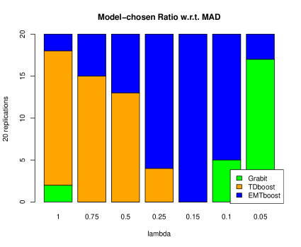
Figure 6: Barplots of model-selection ratio among Grabit, TDboost and EMTboost w.r.t. $\text{Gini}^{b}$ indices under $20$ independent replications when $\lambda$ increases.

Table 5: Comparing Grabit, TDboost and EMTboost with MADs.

	Competing Models
$\lambda$	Grabit	TDboost	EMTboost
$1.00$	$4.248\,(.014)$	$4.129\,(.012)$	$4.067\,(.012)$
$0.75$	$3.879\,(.017)$	$3.679\,(.011)$	$3.622\,(.012)$
$0.50$	$3.345\,(.026)$	$2.994\,(.017)$	$2.928\,(.016)$
$0.25$	$2.439\,(.014)$	$1.945\,(.021)$	$1.766\,(.014)$
$0.15$	$1.720\,(.015)$	$1.489\,(.023)$	$1.309\,(.019)$
$0.10$	$1.265\,(.011)$	$1.100\,(.015)$	$0.986\,(.014)$
$0.05$	$0.714\,(.012)$	$0.578\,(.015)$	$0.402\,(.009)$

We also find that TDboost and EMTboost both outperform Grabit when $\lambda=1$, $0.75$, $0.5$, $0.25$, $0.15$, $0.1$, but Grabit becomes the best when $\lambda=0.05$; interestingly, if we compare MAD results in Table 5, the prediction error of EMTboost becomes the smallest for each $\lambda$. This inconsistent results between the criteria MAD and $\text{Gini}^{b}$ index when $\lambda=0.05$ can be explained by the different learning characteristics of the EMTboost methods and the Grabit methods. To see it more clearly, we compute the MADs on the positive-loss dataset, denoted by $\text{MAD}^{+}$, and zero-loss dataset, denoted by $\text{MAD}^{0}$ seperately, and compute the $\text{Gini}^{a}$ indices on the nonzero dataset, denoted by $\text{Gini}^{a+}$. When $\lambda=0.05$, EMTboost obtains the smallest averaged MAD on zero-loss dataset ($\overline{\text{MAD}^{0}}_{\text{EMTboost}}^{\text{}}=0.146$ < $\overline{\text{MAD}^{0}}_{\text{TDboost}}=0.269$ < $\overline{\text{MAD}^{0}}_{\text{Grabit}}=0.422$), while Grabit obtains the smallest averaged MAD on positive-loss dataset ($\overline{\text{MAD}^{+}}_{\text{EMTboost}}=10.406$ > $\overline{\text{MAD}^{+}}_{\text{TDboost}}=10.297$ > $\overline{\text{MAD}^{+}}_{\text{Grabit}}=9.927$). The $\text{MAD}^{0}$ performance shows that EMTboost captures the zero information much better than TDboost and Grabit. The somewhat worse $\text{MAD}^{+}$ performance of EMTboost when $\lambda=0.05$ can be explained by the deficiency of the nonzero data points (only about $100$ nonzeros comparing with over $3000$ zeros); if we fix the nonzero sample size with under-sampling fraction $\lambda=0.2$, and at the same time, over-sample the zero-loss part with over-sampling fraction $\eta=3$ to obtain about $96\%$ zero proportion, then the averaged $\text{Gini}^{b}$ results summarized in Table 10 in Appendix C.2 indeed show that EMTboost remains to perform competitively compared with the other methods under this large zero proportion setting.

6.   Concluding Remarks

We have proposed and studied the EMTboost model to handle very unbalanced claim data with excessive proportion of zeros. Our proposal overcomes the difficulties that traditional Tweedie model have when handling these common data scenarios, and at the same time, preserves the flexibility of nonparametric models to accomdate complicated nonlinear and high-order interaction relations. We also expect that our zero-inflated Tweedie approach can be naturally extended to high-dimensional linear settings (Qian et al., 2016). It remains interesting to develop extended approaches to subject-specific zero-inflation settings, and provide formal procedures that can conveniently test if zero-inflated Tweedie model is necessary in data analysis compared to its simplified alternatives under both parametric and nonparametric frameworks.

Appendix A Appendix A: Tobit Model (Truncated Normal Distribution)

Suppose the latent variable $Y^{*}$ follows, conditional on covariate x, a Gaussian distribution:

$$Y^{*}|\textbf{x}\sim N(\mu(\textbf{x}),\sigma^{2})$$ (57)

This latent variable $Y^{*}$ is observed only when it lies in an interval $\left[y_{l},y_{u}\right]$. Otherwise, one observes $y_{l}$ or $y_{u}$ depending on whether the latent variable is below the lower threshold $y_{l}$ or above the upper threshold $y_{u}$, respectively. Denoting $Y$ as the observed variable, we can express it as:

$$Y=\begin{cases}y_{l},&\text{if }Y^{*}\leq y_{l},\\ Y^{*},&\text{if }y_{l}<Y^{*}<y_{u},\\ y_{u},&\text{if }y_{u}\leq Y^{*}.\end{cases}$$ (58)

The density of $Y$ is given by:

$$f_{\text{Tobit}}\left(y;\mu(\textbf{x}),\sigma\right) =\Phi\left(\frac{y_{l}-\mu(\textbf{x})}{\sigma}\right)\textbf{I}_{y_{l}}(y)+\left(1-\Phi\left(\frac{y_{u}-\mu(\textbf{x})}{\sigma}\right)\right)\textbf{I}_{y_{u}}(y).$$

$$+\frac{1}{\sigma}\varphi\left(\frac{y-\mu(\textbf{x})}{\sigma}\right)\textbf{I}\left\{y_{l}<y<y_{u}\right\}$$ (59)

Then the expectation of $Y|\textbf{x}$ is given by:

$$\mathbb{E}_{\sigma}\left[y|\textbf{x}\right] =\int_{-\infty}^{+\infty}yf_{\text{Tobit}}\left(y;\mu(\textbf{x}),\sigma\right)dy$$

$$=y_{l}\Phi\left(\alpha\right)+\int_{y_{l}}^{y_{u}}y\frac{1}{\sigma}\varphi\left(\frac{y-\mu(\textbf{x})}{\sigma}\right)dy+y_{u}\left(1-\Phi\left(\beta\right)\right)$$

$$=y_{l}\Phi\left(\alpha\right)+\int_{\alpha}^{\beta}(s\sigma+\mu(\textbf{x}))\varphi\left(s\right)ds+y_{u}\left(1-\Phi\left(\beta\right)\right)$$

$$=y_{l}\Phi\left(\alpha\right)+\sigma\left(\varphi\left(\alpha\right)-\varphi\left(\beta\right)\right)+\mu(\textbf{x})\left(\Phi\left(\beta\right)-\Phi\left(\alpha\right)\right)+y_{u}\left(1-\Phi\left(\beta\right)\right),$$ (60)

where $\alpha=\frac{y_{l}-\mu(\textbf{x})}{\sigma},\beta=\frac{y_{u}-\mu(\textbf{x})}{\sigma}$. And

$$\phi(\xi)=\frac{1}{\sqrt{2\pi}}\exp\left(-\frac{1}{2}\xi^{2}\right)$$ (61)

is the probability density function of the standard normal distribution and $\Phi(\cdot)$ is its cumulative distribution function:

$$\Phi(y)=\int_{-\infty}^{y}\varphi(\xi)d\xi$$ (62)

In simulation 2, the latent variable is truncated by $0$ from below, i.e., $y_{l}=0,y_{u}=\infty$. So we have $\varphi(\beta)=0,\Phi(\beta)=1$. We also set the variance of the Gaussian distribution as $\sigma=1$. Then the expectation of $Y|\textbf{x}$ is given by:

$$\mathbb{E}_{\sigma=1}\left[y|\text{{x}}\right]=\varphi\left(-\mu(\textbf{x})\right)+\mu(\textbf{x})\left(1-\Phi\left(-\mu(\textbf{x})\right)\right).$$ (63)

Appendix B Appendix B: Case 3

In this simulation study, we demonstrate that our EMTboost model can fit the nonclaim dataset well. We consider the data generated from the Tweedie model, with the true target function (47). We generate response $Y$ from the Tweedie distribution $\text{Tw}(\mu,\phi,\rho)$, with $\mu=\exp(F(x_{1},x_{2}))~{},x_{1},x_{2}\sim\text{Unif}(0,1)$ and the index parameter $\rho=1.5$. We find that when the dispersion parameter $\phi$ takes large value in $\mathbb{\mathbb{R}^{+}}$, Tweedie’s zero mass probability $\mathbb{P}(Y_{\text{Tw}}=0)=\exp(-\frac{1}{\phi}\frac{\mu^{2-\rho}}{2-\rho})$ gets closer to $1$. So we choose three large dispersion values $\phi\in\left\{20,30,50\right\}$.

We generate $n=500$ observations $\{\textbf{x}_{i},y_{i}\}_{i=1}^{n}$ for training and $n^{\prime}=1000$ for testing, and fit the training data using Grabit, TDboost and EMTboost models. For all three models, five-fold cross-validation is adopted and the shrinkage factor $\nu$ is set as $0.001$. The profile likelihood method is used.

The discrepancy between the predicted loss and the expected true loss in criteria MAD and $\text{Gini}^{b}$ index are shown in Table 6 and Table 7, which are averaged over 20 independent replications for each $\phi$. Table 6 shows that EMTboost obtains the smallest MAD. In terms of $\text{Gini}^{b}$ indices, EMTboost is also chosen as the “best” model for each $\phi$.

In this setting, $\mathbb{P}(Y_{\text{Tw}}=0)\approx 0.83,0.88,0.91$, which means that all the customers are generally very likely to have no claim. The assumption of our EMTboost model with a general exact zero mass probability coincides with this data structure. Its zero mass probability estimation $1-\widehat{q}$ is $0.863$, $0.909$ and $0.943$ respectively, showing that EMTboost learns this zero part of information quite well. As a result, EMTboost performs no worse than TDboost, which is based on the true model assumption.

Table 6: Simulation results for case 3 with MADs.

	Competing Models
$\phi$	Grabit	TDboost	EMTboost
$20$	$2.499\,(.072)$	$2.465\,(.057)$	$2.449\,(.054)$
$30$	$2.442\,(.068)$	$2.492\,(.060)$	$2.442\,(.060)$
$50$	$2.553\,(.091)$	$2.560\,(.082)$	$2.544\,(.080)$

Table 7: Simulation results for case 3 with $\text{Gini}^{b}$ indices.

	Competing premium
Base premium	Grabit	TDboost	EMTboost
	$\phi=20$
Grabit	$0$	$8.205\,(3.492)$	$8.052\,(3.471)$
TDboost	$4.487\,(2.462)$	$0$	$4.104\,(2.283)$
EMTboost	$\bm{3.153}\,(1.982)$	$2.347\,(1.656)$	$0$
	$\phi=30$
Grabit	$0$	$4.273\,(3.447)$	$3.244\,(3.411)$
TDboost	$4.017\,(3.257)$	$0$	$3.454\,(3.191)$
EMTboost	$\bm{1.404}\,(2.730)$	$0.846\,(2.403)$	$0$
	$\phi=50$
Grabit	$0$	$5.452\,(4.806)$	$10.362\,(4.801)$
TDboost	$3.479\,(3.654)$	$0$	$2.476\,(3.899)$
EMTboost	$-0.836\,(2.785)$	$\bm{1.031}\,(3.354)$	$0$

Appendix C Appendix C: Real Data

C.1.   Implemented EMTboost: Penalization on $q$

When fitting the EMTboost model, we want to avoid the situation that the Tweedie portion probability estimation $\widehat{q}$ degenerates to $0$. So we add a regularization term $r\log\left(1-q\right)$ to the Q-function, as equation (39) in Section 3.2. We choose an increasing sequence of penalty parameter $\log_{10}\left(r\right)\in\left\{-2,\cdots,1\right\}_{41}$, and use the strategy of “warm start” to improve the computation efficiency, i.e., setting the current solution $\left(\widehat{\mu}\left(r_{l}\right),\widehat{\phi}\left(r_{l}\right),\widehat{q}\left(r_{l}\right)\right)$ as the initialization for the next solution $\left(\widehat{\mu}\left(r_{l+1}\right),\widehat{\phi}\left(r_{l+1}\right),\widehat{q}\left(r_{l+1}\right)\right)$.

We use this implemented EMTboost model to train the penalized solution paths with respect to the sequence of penalty parameter $r$ on the extremely zero-inflated training data $\left(\lambda=0.05\right)$ under $20$ independent replications, and then apply the estimators to the testing data to compute the discrepancy under MAD. We also compute the MADs on zero-loss dataset ($\text{MAD}^{0}$) and positive-loss dataset ($\text{MAD}^{+}$) seperately, and the $\text{Gini}^{a}$ indices on positive-loss dataset ($\text{Gini}^{a+}$). Table 8 and Figure 7 shows the implemented EMTboost MAD path w.r.t. the logrithm of a sequence of penalty parameter $r$.

Table 8: Implemented EMTboost ($\lambda=0.05$) results with MADs, $\text{MAD}^{0}$s and $\text{MAD}^{+}$s.

$\log(r)$	$-2.00$	$-1.10$	$-0.65$	$0.25$	$0.70$
MAD	$0.432\,(0.047)$	$0.377\,(0.036)$	$0.351\,(0.033)$	$0.330\,(0.032)$	$0.328\,(0.031)$
$\text{MAD}^{0}$	$0.114\,(0.026)$	$0.054\,(0.011)$	$0.026\,(0.005)$	$0.004\,(0.001)$	$0.002\,(0.000)$
$\text{MAD}^{+}$	$10.452\,(1.017)$	$10.527\,(1.017)$	$10.560\,(1.017)$	$10.587\,(1.017)$	$10.590\,(1.017)$

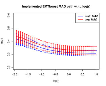
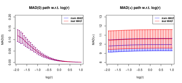
Figure 7: Implemented EMTboost ($\lambda=0.05$) results: MAD error path with its one standard deviation when increasing regularization parameter $r$. The blue lines are the training error lines, and the red ones are the testing error lines. Top figure: averaged MAD drops when penalty parameter increases. Bottom left: averaged $\text{MAD}^{0}$ and its standard deviation drop remarkably and approximate $0$ when $r$ increases. Bottom right: averaged $\text{MAD}^{+}$ is flat and increases a little when $r$ increases. All the averaged testing MADs are within one standard deviation of the averaged training MADs.

Table 9 shows the results of Grabit, TDboost, EMTboost, and implemented EMTboost $\left(r=1/6\right)$. Implemented EMTboost performs the worst in $\text{Gini}^{a}$, $\text{Gini}^{a+}$ and $\text{MAD}^{+}$, but the best in MAD and $\text{MAD}^{0}$.

Table 9: Comparing Grabit, TDboost, EMTboost and Implemented EMTboost ($r=1/6$) with $\text{Gini}^{a}$ indices and MADs.

$\lambda=0.05$	Grabit	TDboost	EMTboost	Implemented EMTboost
$\widehat{q}$	-	-	$0.697\,(.018)$	$0.132\,(.003)$
$\text{Gini}^{a}$	$0.415\,(.023)$	$0.134\,(.040)$	$0.238\,(.033)$	$0.261\,(.033)$
$\text{Gini}^{a+}$	$0.104\,(.030)$	$-0.116\,(.039)$	$-0.164\,(.031)$	$-0.103\,(.040)$
MAD	$0.714\,(.012)$	$0.578\,(.015)$	$0.482\,(.013)$	$0.356\,(.008)$
$\text{MAD}^{0}$	$0.422\,(.009)$	$0.269\,(.012)$	$0.146\,(.008)$	$0.032\,(.002)$
$\text{MAD}^{+}$	$9.927\,(.223)$	$10.287\,(.226)$	$10.406\,(.228)$	$10.551\,(.227)$

C.2.   Resampleing: Under-sampling Fraction $\lambda=0.2$ and Over-sampling Fraction $\eta=3$

We control the nonzero sample size in real application by under-sampling the nonzero-loss data set with fraction $\lambda=0.2$ and over-sampling the zero-loss data with fraction $\eta=3$, generating a data set containing $95.9\%$ zeros. Following the training and testing procedure in Section 5, Table 10shows that EMTboost has the smallest of the maximal (averaged) $\text{Gini}^{b}$ indices, thus is chosen as the “best” model.

Table 10: Grabit, TDboost, EMTboost $\text{Gini}^{b}$ indices with $\lambda=0.2$ and $\eta=3$.

$\lambda=0.2,\eta=3$	Competing Premium
Base Premium	Grabit	TDboost	EMTboost
Grabit	$0$	$23.872\,(3.928)$	$35.616\,(2.655)$
TDboost	$-4.822\,(2.822)$	$0$	$27.234\,(2.152)$
EMTboost	$\bm{-5.583}\,(1.599)$	$-14.806\,(1.681)$	$0$

References

- Breiman (1999) Breiman, L. (1999), “Prediction games and arcing algorithms,” Neural computation, 11, 1493–1517.
- Breiman et al. (1998) Breiman, L. et al. (1998), “Arcing classifier (with discussion and a rejoinder by the author),” The annals of statistics, 26, 801–849.
- Brent (2013) Brent, R. P. (2013), Algorithms for minimization without derivatives, Courier Corporation.
- Cragg (1971) Cragg, J. G. (1971), “Some statistical models for limited dependent variables with application to the demand for durable goods,” Econometrica: Journal of the Econometric Society, 829–844.
- Dunn and Smyth (2005) Dunn, P. K. and Smyth, G. K. (2005), “Series evaluation of Tweedie exponential dispersion model densities,” Statistics and Computing, 15, 267–280.
- Frees et al. (2016) Frees, E., Lee, G., and Yang, L. (2016), “Multivariate frequency-severity regression models in insurance,” Risks, 4, 4.
- Frees et al. (2011) Frees, E. W., Meyers, G., and Cummings, A. D. (2011), “Summarizing insurance scores using a Gini index,” Journal of the American Statistical Association, 106, 1085–1098.
- Frees et al. (2014) — (2014), “Insurance ratemaking and a Gini index,” Journal of Risk and Insurance, 81, 335–366.
- Freund and Schapire (1997) Freund, Y. and Schapire, R. E. (1997), “A decision-theoretic generalization of on-line learning and an application to boosting,” Journal of computer and system sciences, 55, 119–139.
- Friedman et al. (2001) Friedman, J., Hastie, T., and Tibshirani, R. (2001), The elements of statistical learning, vol. 1, Springer series in statistics New York, NY, USA:.
- Friedman et al. (2000) Friedman, J., Hastie, T., Tibshirani, R., et al. (2000), “Additive logistic regression: a statistical view of boosting (with discussion and a rejoinder by the authors),” The annals of statistics, 28, 337–407.
- Friedman (2001) Friedman, J. H. (2001), “Greedy function approximation: a gradient boosting machine,” Annals of statistics, 1189–1232.
- Friedman (2002) — (2002), “Stochastic gradient boosting,” Computational Statistics & Data Analysis, 38, 367–378.
- Hall (2000) Hall, D. B. (2000), “Zero-inflated Poisson and binomial regression with random effects: a case study,” Biometrics, 56, 1030–1039.
- Hastie and Tibshirani (1990) Hastie, T. J. and Tibshirani, R. J. (1990), “Generalized additive models, volume 43 of Monographs on Statistics and Applied Probability,” .
- Jørgensen (1987) Jørgensen, B. (1987), “Exponential dispersion models,” Journal of the Royal Statistical Society. Series B (Methodological), 127–162.
- Jørgensen and Paes De Souza (1994) Jørgensen, B. and Paes De Souza, M. C. (1994), “Fitting Tweedie’s compound Poisson model to insurance claims data,” Scandinavian Actuarial Journal, 1994, 69–93.
- Lambert (1992) Lambert, D. (1992), “Zero-inflated Poisson regression, with an application to defects in manufacturing,” Technometrics, 34, 1–14.
- Mildenhall (1999) Mildenhall, S. J. (1999), “A systematic relationship between minimum bias and generalized linear models,” in Proceedings of the Casualty Actuarial Society, vol. 86, pp. 393–487.
- Mullahy (1986) Mullahy, J. (1986), “Specification and testing of some modified count data models,” Journal of econometrics, 33, 341–365.
- Murphy et al. (2000) Murphy, K. P., Brockman, M. J., and Lee, P. K. (2000), “Using generalized linear models to build dynamic pricing systems,” in Casualty Actuarial Society Forum, Winter, Citeseer, pp. 107–139.
- Nelder and Wedderburn (1972) Nelder, J. and Wedderburn, R. (1972), “Generalized Linear Models,” Journal of the Royal Statistical Society. Series A (General), 370–384.
- Qian et al. (2016) Qian, W., Yang, Y., and Zou, H. (2016), “Tweedie’s compound Poisson model with grouped elastic net,” Journal of Computational and Graphical Statistics, 25, 606–625.
- Sandri and Zuccolotto (2008) Sandri, M. and Zuccolotto, P. (2008), “A bias correction algorithm for the Gini variable importance measure in classification trees,” Journal of Computational and Graphical Statistics, 17, 611–628.
- Sigrist and Hirnschall (2017) Sigrist, F. and Hirnschall, C. (2017), “Grabit: Gradient Tree Boosted Tobit Models for Default Prediction,” arXiv preprint arXiv:1711.08695.
- Smyth and Jørgensen (2002) Smyth, G. K. and Jørgensen, B. (2002), “Fitting Tweedie’s compound Poisson model to insurance claims data: dispersion modelling,” ASTIN Bulletin: The Journal of the IAA, 32, 143–157.
- Tobin (1958) Tobin, J. (1958), “Estimation of relationships for limited dependent variables,” Econometrica: journal of the Econometric Society, 24–36.
- Tweedie (1984) Tweedie, M. (1984), “An index which distinguishes between some important exponential families,” 579, 6o4.
- Wood (2006) Wood, S. N. (2006), Generalized additive models: an introduction with R, Chapman and Hall/CRC.
- Yang et al. (2017) Yang, Y., Qian, W., and Zou, H. (2017), “Insurance premium prediction via gradient tree-boosted Tweedie compound Poisson models,” Journal of Business & Economic Statistics, 1–15.
- Ye et al. (2018) Ye, C., Zhang, L., Han, M., Yu, Y., Zhao, B., and Yang, Y. (2018), “Combining Predictions of Auto Insurance Claims,” arXiv preprint arXiv:1808.08982.
- Yip and Yau (2005) Yip, K. C. and Yau, K. K. (2005), “On modeling claim frequency data in general insurance with extra zeros,” Insurance: Mathematics and Economics, 36, 153–163.
- Zhang et al. (2005) Zhang, T., Yu, B., et al. (2005), “Boosting with early stopping: Convergence and consistency,” The Annals of Statistics, 33, 1538–1579.
- Zhang (2011) Zhang, W. (2011), “cplm: Monte Carlo EM algorithms and Bayesian methods for fitting Tweedie compound Poisson linear models,” R package version 0.2-1, URL http://CRAN. R-project. org/package= cplm.