An improved implicit sampling for Bayesian inverse problems of multi-term time fractional multiscale diffusion models

ABSTRACT

This paper presents an improved implicit sampling method for hierarchical Bayesian inverse problems. A widely used approach for sampling posterior distribution is based on Markov chain Monte Carlo (MCMC). However, the samples generated by MCMC are usually strongly correlated. This may lead to a small size of effective samples from a long Markov chain and the resultant posterior estimate may be inaccurate. An implicit sampling method proposed in [11] can generate independent samples and capture some inherent non-Gaussian features of the posterior based on the weights of samples. In the implicit sampling method, the posterior samples are generated by constructing a map and distribute around the MAP point. However, the weights of implicit sampling in previous works may cause excessive concentration of samples and lead to ensemble collapse. To overcome this issue, we propose a new weight formulation and make resampling based on the new weights. In practice, some parameters in prior density are often unknown and a hierarchical Bayesian inference is necessary for posterior exploration. To this end, the hierarchical Bayesian formulation is used to estimate the MAP point and integrated in the implicit sampling framework. Compared to conventional implicit sampling, the proposed implicit sampling method can significantly improve the posterior estimator and the applicability for high dimensional inverse problems. The improved implicit sampling method is applied to the Bayesian inverse problems of multi-term time fractional diffusion models in heterogeneous media. To effectively capture the heterogeneity effect, we present a mixed generalized multiscale finite element method (mixed GMsFEM) to solve the time fractional diffusion models in a coarse grid, which can substantially speed up the Bayesian inversion. Using the improved implicit sampling, we carry out a few numerical examples to effectively identify various unknown inputs in these models.

keywords: Bayesian inversion, improved implicit sampling, mixed GMsFEM, multi-term time fractional diffusion models

1 Introduction

The fractional diffusion equations have been widely used in modelling of the anomalous phenomenon, such as fractal media, chemistry, and material physics [8, 6, 25, 31]. The time fractional diffusion equations are obtained from the standard diffusion equations through replacing the integer-order time derivative with a fractional derivative, which can be derived from random walk models or generalized master equations. The diffusion process for inhomogeneous anisotropic media modelling by time fractional diffusion equations is also very common in physics [9, 15, 7]. In order to make the modelling more precise, fractional diffusion equations with multi-term time fractional derivatives have been investigated in recent years [29, 30]. If all parameters in the fractional models are given, there are many methods to solve the forward model [22, 45]. However, in practice, there are many inputs unknown in the fractional model, such as the multi-fractional derivatives, the diffusion field and the reaction field. Thus, identification of the unknown inputs in fractional diffusion models lead to inverse problems. To the authors’ best knowledge, there are only few works focused on the inverse problems for multi-term time fractional diffusion model, such as Jiang et al. [20] for determining the source term, Sun et al. [40] for identifying reaction coefficient, and Li et al. [28] for recovering fractional orders and reaction coefficient simultaneously.

The estimation of unknown parameters from limited and noisy measurement data is a big challenge in science and engineering. Uncertainty in model inputs leads to the uncertainty in model predictions, which can in turn have a great impact on experimental design and decision-making. In general, the inverse problems are often ill-posed because of the limited indirect and noisy data. One of the most popular approaches to estimate the unknown parameters is to minimize a cost function involving the misfit between the measurement data and the simulated response based on a regularization term. This is usually called Tikhonov regularization [37]. Iterative methods are used to solve the minimization problems. However, these deterministic approaches usually only generate a point estimate of the unknown parameters, without quantifying the uncertainty in parameters. To treat this situation, the Bayesian statistical approach [16, 23, 21, 38] is often used to solve the inverse problems.

The Bayesian inference provides a natural mechanism for learning from the measurement data by incorporating some prior information and has distinct features over classical deterministic regularization methods. One can obtain the marginalizing, moments ,or confidence intervals through characterizing the posterior distribution. However, only in some special cases, the posterior may be in a closed form. Even when the prior and likelihood are Gaussian, the posterior may be non-Gaussian due to the nonlinearity of the forward operator. The most common choice for exploring the posterior is Markov chain Monte Carlo (MCMC) [16], which generates a serial of samples to evaluate the statistical information. However, MCMC has some drawbacks. For instance, MCMC usually requires millions of samples to estimate the statistical information. This means that a large number of forward model simulations need to be computed. In addition, the resultant samples may be correlated and the size of effective samples is small. It is also difficult to diagnose the convergence of MCMC in practice.

For computationally expensive forward models, sampling using MCMC may be infeasible. Hence, it is necessary to find some other sampling methods with a small computation burden. The ensemble-based method is one of the approaches and give an approximation of the posterior. The typical ensemble methods include linearization around the maximum a posterior distribution (LMAP) [16], randomized maximum likelihood (RML) [24], and ensemble Kalman filter (ENKF) [3, 4], etc.. These methods may be inaccurate because they can be regarded as Gaussian approximations of the posterior. In addition, there exist some other methods based on optimization to improve the performance of sampling in the frame of Bayesian inference, such as randomize-then-optimize (RTO) [5] and optimal map [34]. RTO produces candidate samples from solving a randomly perturbed optimization problem, which acts as a Metropolis proposal. And [44] extends RTO to some cases with non-Gaussian prior. The optimal map needs to construct a map that push the prior measure to posterior measure. However, the construction of the map is often computationally expensive.

An alternative to the above approaches is importance sampling [3, 16], which is a sampling method without any Gaussian assumption. The idea is to draw samples from another easy-sampling importance function with a weight of each sample instead of drawing samples from the target distribution itself, which is usually difficult to explore directly. But the effective sample size [3, 16] may be very small in the conventional importance sampling if the variance of the weights are large. This situation is called filter degeneracy or ensemble collapse [41]. It is critical to carefully select the important function, which can in turn influence the weights. Recently, a method called implicit sampling was proposed in [11] and studied for inverse problems [10, 32, 33, 39]. The implicit sampling method acts as a special formulation of importance sampling to improve sample performance by providing an importance function based on optimization. In order to make samples concentrate on the region with high probability, implicit sampling firstly solve a minimization problem to obtain the MAP point. Then a serial of samples can be generated through solving a nonlinear algebraic equation with a random right hand term. The implicit sampling shares some similarities with LMAP. But the implicit sampling can capture some non-Gaussian information of the posterior based on the weight of each sample compared with LMAP. Moreover, the implicit sampling produces independent samples, which greatly reduce the autocorrelation of samples and avoid the long burn-in process in MCMC. However, there still exist many shortcomings in the conventional implicit sampling. For example, the conventional implicit sampling may still cause sample degeneracy. The implicit sampling is stilled considered for Gaussian prior in most of the previous works [11, 10, 32, 33, 39].

In this paper, we present an improved implicit sampling method and its application with some non-Gaussian priors. When the dimension of unknown parameter is high and the model structure is complicated, the weights of the conventional implicit sampling may cause excessive concentration of samples and lead to ensemble collapse, which may give a poor estimation of the posterior. To overcome the issue, we propose a new weight formulation, which can properly balance the weights of samples. Meanwhile, this new formulation of weight can still retain the original weight order. In practice, the prior information often involves unknown parameters. Hierarchical Bayesian model [23] is necessary to treat this situation. In this paper, we consider the hierarchical Bayesian model when making the MAP estimate in implicit sampling. In addition, we use a Laplace prior for the inputs with heterogeneous property depending on the knowledge of sparsity regularization [24, 27].

For the multi-term time fractional diffusion models in heterogeneous media, there may exist some multiple scales and high contrast feature in the diffusion field. Direct simulating the multiscale models may be very computationally expensive. But Bayesian inversion requires to simulate the forward model many times. Hence, it is necessary to use a suitable model reduction for multiscale models to significantly improve the computation efficiency. It is well known that Generalized Multiscale Finite Element Method (GMsFEM) [13, 14, 18] can efficiently solve the multiscale models in a coarse grid. GMsFEM aims at dividing the computation into offline and online steps. One entails constructing the offline space in order to provide a good approximation of the solution with fewer basis functions. The offline space is established depending on the spectral decomposition of the snapshot space, which can be obtained by solving some local problems. In this paper, we utilize mixed GMsFEM [12, 35] to solve the multi-term time fractional multiscale diffusion models. The mixed GMsFEM can give accurate flux information. The measurement data are the flux information collected at the boundary of the spatial domain.

The paper is organized as follows. In Section 2, we introduce the implicit sampling in Bayesian framework, which includes the approaches to compute the MAP point for different prior information. In Section 3, we introduce the multi-term time fractional diffusion model and then construct the reduced model using mixed GMsFEM. Some numerical results are presented in Section 4 to show the performance of the proposed method. The paper ends with some conclusions and comments in Section 5.

2 Bayesian inference based on implicit sampling

We begin with describing the Bayesian framework and denoting some notions for the paper. We consider the following general model

$$\mathcal{B}(\theta,u)=0\ \ \text{in}\ \ \Omega,$$ (2.1)

which can represent a PDE modeling some physical problems. If the model inputs $\theta$ are available, the model output $u$ can be obtained by numerical simulation. Let $\theta\in\mathds{R}^{m}$. In Bayesian inversion, the unknown parameters and measurement data are usually regarded as random variables. Let $(\mathcal{S},\mathcal{F},\mathds{P})$ be a measure space, where $\mathcal{S}$ is the sampling space, $\mathcal{F}$ is the $\sigma\text{-field}$ and $\mathds{P}$ is the probability measure. Then $p(\theta)=d\mu_{0}/d\theta$ is the density of $\theta$ with respect to Lebesgue measure, where $\mu_{0}$ is a prior measure. According to Bayes’s rule, the posterior probability can be obtained by

$$p(\theta|d)=\frac{p(d|\theta)p(\theta)}{\beta},$$ (2.2)

where the function $p(d|\theta)$ is the likelihood function and $\beta$ is the evidence or marginal likelihood $\beta=\int p(d|\theta)p(\theta)d\theta$. Assume that $\theta^{*}\in\mathds{R}^{m}$ is the reference parameter. We assume that the measurement data is generated by

$$d=H(\theta^{*})+\epsilon,$$ (2.3)

where the function $H:\mathds{R}^{m}\rightarrow\mathds{R}^{n}$ denotes the parameter-to-observation (or forward) map according to model (2.1) and $\epsilon$ is a random variable independent of $\theta$. Generally, we assume $\epsilon\sim N(0,\sigma^{2}\text{I})$, where $\text{I}\in\mathds{R}^{n\times n}$ is the identity matrix. In Bayesian inverse problems, one intends to explore the posterior, which relies on the sparse measurement data $d$ and some prior information $p(\theta)$.

2.1 Hierarchical Bayesian formulation

Under the above assumptions, it can be concluded that the likelihood function has the following form

$$p(d|\theta)\propto(\sigma^{2})^{-n/2}\exp(-\frac{\|H(\theta)-d\|^{2}_{2}}{2\sigma^{2}}).$$

The prior $p(\theta)$ depends on the knowledge of the unknown inputs and plays a critical role on exploring the posterior. A versatile choice for $p(\theta)$ is Markov random field (MRF), i.e.

$$p(\theta)\propto\lambda^{\frac{m}{2}}\exp(-\frac{\lambda}{2}\|\theta\|^{2}_{2}).$$

If $\lambda$ is known, the posterior density $p(\theta|d)$ can be obtained as

$$p(\theta|d)\propto\lambda^{\frac{m}{2}}\exp(-\frac{\|H(\theta)-d\|^{2}_{2}}{2\sigma^{2}})\exp(-\frac{\lambda}{2}\|\theta\|^{2}_{2}).$$

The posterior density $p(\theta|d)$ provides the complete distribution of $\theta$ relying on the observations $d$. We can compute the MAP point, ${\theta}_{MAP}:=\arg\max_{\theta}p(\theta|d)$, which is equivalent to the following minimization problem

$$\theta_{MAP}=\arg\min\big{\{}\|H(\theta)-d\|^{2}_{2}+\mu\|\theta\|^{2}_{2}\big{\}},$$

where $\mu=\lambda\sigma^{2}$ plays the role of regularization parameter in inverse problems. However, as we know, it is not an easy task to ascertain the regularization parameter, especially in nonlinear inverse problems. Fortunately, the hierarchical Bayesian model [16, 23] can provide an effective and flexible way to overcome the difficulty. In hierarchical Bayesian framework, $\lambda$ can be regarded as a hyper-parameter, i.e., we can choose a hyper-prior $p(\lambda)$ for it. Then the posterior density can be written as

$$p(\theta,\lambda)\propto p(d|\theta)p(\theta)p(\lambda).$$

A common method to choose hyper-prior $p(\lambda)$ is using conjugate priors. If we use Gamma distribution as the hyper-prior for $\lambda$, then the posterior density becomes

$$p(\theta,\lambda|d)\propto\lambda^{\frac{m}{2}}\exp(-\frac{\|H(\theta)-d\|^{2}_{2}}{2\sigma^{2}})\exp(-\frac{\lambda}{2}\|\theta\|^{2}_{2})\lambda^{a-1}\exp(-b\lambda),$$ (2.4)

where $\lambda\thicksim Gamma(a,b)$ [16]. Then the MAP estimate for (2.4) can be computed by minimizing the following functional

$$\mathcal{M}(\theta,\lambda)=\frac{\|H(\theta)-d\|^{2}_{2}}{2\sigma^{2}}+\frac{\lambda}{2}\|\theta\|^{2}_{2}+b\lambda-(\frac{m}{2}+a-1)\ln\lambda.$$ (2.5)

However, when solving the forward model, it usually depends on the spatially discretized grid system. Thus if the random vector $\theta$ is grid-based, its dimension may be very high. This will result in the instability and inefficiency of the numerical algorithms. Therefore, the reduction of the dimension of parameter space is necessary. Let the parameter $\theta$ can be represented by

$$\log\theta=\Phi\textbf{v}+\kappa,$$ (2.6)

where $\textbf{v}=[v_{1},v_{2},\cdots,v_{l}]$ are the coefficients under the base matrix $\Phi\in\mathbb{R}^{m\times l}$ and $\kappa$ is a fixed constant vector. Thus the parameter-to-observation map $H(\theta)$ can be expressed by $H(\textbf{v})$. For convenience, we use $\textbf{v}^{*}$ to indicate the reference parameter. We can use the augmented-Tikhonov method [23] to get the MAP estimate. Table 1 describes the augmented-Tikhonov method when the prior for v is assumed to be Gaussian.

Table 1: Augmented-Tikhonov algorithm

Input: The noise level $\sigma$, the maximum iterations $R$ and the precision $eps$ .

Output: $\textbf{v}_{k}=(v_{1}^{k},...,v_{l}^{k})^{T}.$

1. $\bf{Initialize}$ Set k=0 and give the initial value $\textbf{v}_{0}$ and $\mu_{0}$;

2. Settle the forward problem and obtain the additional data $d=H(\textbf{v}^{*})+\epsilon$;

3. $\bf{While}$ $k<R$

4. Compute $h_{k}=(\bar{H}^{T}\bar{H}+\mu_{k-1}I)^{-1}\bar{H}^{T}(d-H(\textbf{v}_{k-1}))$, where $\bar{H}$ is the sensitivity matrix;

5. Update $\textbf{v}_{k}$ by $\textbf{v}_{k}=\textbf{v}_{k-1}+h_{k};$

6. Update the hyper-parameter $\lambda_{k}$ by $\lambda_{k}=\frac{\frac{l}{2}+a-1}{\frac{1}{2}\|\textbf{v}_{k}\|^{2}+b}$ and set $\mu_{k}=\lambda_{k}\sigma^{2}$;

7. $k\leftarrow k+1$;

8. $\bf{Terminate}$ if $\|h_{k}\|<eps$;

9. $\bf{end}$

2.2 MAP estimate with Laplace prior

In this subsection, we consider a non-Gaussian prior case, Laplace prior, which is often used in describing realistic geologic system [24, 27]. Assume the grid-based parameter $\log\theta$ has an approximation formulation as (2.6). A common measure of sparsity of the vector v involves the number of nonzero entries in v, i.e., $\|\textbf{v}\|=\sharp\{i,v_{i}\neq 0\}$. The sparse reconstruction aims at recovering the sparse vector v based on the measurement data $d$. The original sparse inversion problem can be represented as

$$\min\|\textbf{v}\|_{0}\ \ \ s.t.\ \ H(\textbf{v})=d.$$

The exact solution to the above $l_{0}$-$norm$ minimization problem is usually NP-hard. As an alternative, one can find a sparse solution under some mild condition by solving the following problem

$$\min\|\textbf{v}\|_{1}\ \ \ s.t.\ \ H(\textbf{v})=d.$$ (2.7)

The constrained optimization problem (2.7) can be represented by the following unconstrained optimization problem

$$\min\mathcal{J}(\textbf{v})=\|H(\textbf{v})-d\|_{2}^{2}+\mu\|\textbf{v}\|_{1},$$ (2.8)

where $\mu$ acts as the regularization parameter.

For Bayesian inverse problems, if we select the Laplace distribution as a prior for v, i.e., $p(\textbf{v})=\frac{\lambda}{2}\exp(-\lambda\|\textbf{v}\|_{1})$, then the posterior density is

$$p(\textbf{v}|d)\propto\exp(-\mathcal{M}(\textbf{v})),\quad\text{where}\quad\mathcal{M}(\textbf{v})=\frac{\|H(\textbf{v})-d\|_{2}^{2}}{2\sigma^{2}}+\lambda\|\textbf{v}\|_{1}.$$ (2.9)

Let $\mu=2\lambda\sigma^{2}$, then we can find the MAP estimate of $p(\textbf{v}|d)$ by solving the minimization problem (2.8). However, since the derivative of the function $\mathcal{J}(\textbf{v})$ is not defined at the origin, we use the iteratively reweighted approach [27, 24] to solve (2.8), which is widely used in compressive sensing. As mentioned above, the cost function in the iteratively reweighted approach is

$$\min\mathcal{J}(\textbf{v})=\|H(\textbf{v})-d\|_{2}^{2}+\mu\|\textbf{v}\|_{W}^{2},$$ (2.10)

where $W$ is a diagonal weighting matrix generated by the vector $w=[(v_{1}^{2}+\varepsilon)^{-\frac{1}{2}},\cdots,(v_{l}^{2}+\varepsilon)^{-\frac{1}{2}}]$ with a small constant $\varepsilon>0$, and $\|\textbf{v}\|^{2}_{W}=\textbf{v}^{T}W\textbf{v}$. Note that when $\varepsilon=0$, the term $\|\textbf{v}\|^{2}_{W}$ actually equals to $\|\textbf{v}\|_{1}$. We have obtained a similar formalization of the minimization function for the Gaussian prior and Laplace prior. Based on (2.10), the iteratively reweighted approach is listed in Table 2.

Table 2: The iteratively reweighted approach

Input: The noise level $\sigma$, the regularization parameter $\mu$, the maximum iterations $R$,

and the positive constant $\varepsilon$.

Output: $\textbf{v}_{k}=(v_{1}^{k},...,v_{l}^{k})^{T}.$

1. $\bf{Initialize}$ Set k=0 and give the initial value $\textbf{v}_{0}$ and $\mu_{0}$;

2. Settle the forward problem and obtain the additional data $d=H(\textbf{v}^{*})+\epsilon$;

3. $\bf{While}$ $k<R$

4. Update the matrix $W$;

5. Compute $\textbf{v}_{k}=(\bar{H}^{T}\bar{H}+\mu W)^{-1}\bar{H}^{T}(d-H(\textbf{v}_{k-1})+\bar{H}\textbf{v}_{k-1})$,

where $\bar{H}$ is the sensitivity matrix;

6. $\bf{end}$

The above approaches focus on the point estimate (MAP) of unknown inputs from the perspective of variation formulation. However, it is still not enough to characterize the uncertainty of the unknown parameters and the uncertainty propagation of model response. As we know, the most popular method to explore the posterior by samples is Markov chain Monte Carlo (MCMC) [16]. Based on large number of samples generated by MCMC, some statistical information can be estimated to approximate the target distribution. However, MCMC usually needs a lot of samples to estimate the parameter and it is also difficult to diagnose if the chain has converged to the posterior distribution. To overcome these difficulties, we introduce an improved implicit sampling method to efficiently explore the posterior samples.

2.3 Improved implicit sampling

In this subsection, we present implicit sampling, which shares some idea with importance sampling. To this end, we first describe the basic idea of importance sampling [16, 41]. Importance sampling methods can be regarded as multi-step sampling generation techniques. Suppose that we want to sample from a probability density function (pdf) $\rho(\theta)$. However, it is not always an easy task to draw from $\rho(\theta)$ directly. In importance sampling, one first needs to select another easy-sampling pdf $q(\theta)$ and then provides some sort of correction mechanism to draw the samples from $q(\theta)$ to approximate the interest distribution $\rho(\theta)$. As an example, we consider the integration of the form

$$I=\int f(\theta)\rho(\theta)d\theta.$$

If the samples $\{\theta_{i}\}_{i=1}^{N_{s}}$ can be obtained from $\rho(\theta)$ directly, then we can use the simple Monte Carlo (MC) estimator [16] to calculate the integral:

$$I\approx\frac{1}{N_{s}}\sum_{i=1}^{N_{s}}f(\theta_{i})\ \ \text{as}\ \ N_{s}\rightarrow\infty.$$

If $\rho(\theta)$ is not easy for sampling, the integral can be rewritten in the following form with the auxiliary density $q(\theta)$:

$$I=\int f(\theta)\rho(\theta)dx=\int f(\theta)\frac{\rho(\theta)}{q(\theta)}q(\theta)d\theta.$$

Draw samples $\theta_{i}\sim q(\theta)$, and then

$$I\approx\frac{1}{N_{s}}\sum_{i=1}^{N_{s}}f(\theta_{i})\omega_{i}\ \ \text{as}\ \ N_{s}\rightarrow\infty,$$

where the weight $\omega_{i}=\frac{\rho(\theta_{i})}{q(\theta_{i})}$. The auxiliary density must be chosen carefully. In particular, when the interest distribution is the posterior $p(\theta|d)$ and the auxiliary density is chosen as the prior $p(\theta)$, then according to Baye’s rule,

$$E(f(\theta))=\int f(\theta)p(\theta|d)d\theta\approx\sum_{i=1}^{N_{s}}\omega_{i}f(\theta_{i}),$$ (2.11)

where $\theta_{i}\sim p(\theta)$ and $\omega_{i}=\frac{p(d|\theta_{i})}{\sum_{i=1}^{N}p(d|\theta_{i})}$. However, when the prior and likelihood have disjoint support or the prior is too broad, the estimate in (2.11) is not accurate. Implicit sampling can effectively improve the conventional importance sampling in this situation. Based on [33], we give a brief introduction to the implicit sampling, which concentrate on the region with the high posterior probability.

Let

$$F(\theta)=-\log(p(d|\theta)p(\theta)).$$

First, we need to find the MAP estimate by minimizing the negative logarithm of the posterior. Suppose that

$$\theta_{MAP}=\operatorname*{arg\,min}_{\theta}F(\theta),\quad\phi_{F}=\min F(\theta).$$

Then we intend to select an auxiliary function to efficiently draw samples from high probability region, i.e., near the MAP point. To this end, we can use standard Gaussian distribution

$$\bar{q}(\xi)\varpropto\exp(-\frac{1}{2}\xi^{T}\xi)$$

to play the role of the easy-sampling density. Denote $G(\xi)=\frac{1}{2}\xi^{T}\xi$ and $\phi_{G}=\min G(\xi)$, then we solve the following nonlinear algebraic equation:

$$F(\theta)-\phi_{F}=G(\xi)-\phi_{G}.$$ (2.12)

It can be concluded that the left-hand of (2.12) tends to be small since samples drawn from $\bar{q}(\xi)$ can make $G(\xi)$ close to $\phi_{G}$. By solving the above algebraic equation for a series of samples $\xi$, we can obtain the samples located around the MAP point. Based on this idea, we define a map $\mathcal{A}:\xi\rightarrow\theta$ to find the solution. The pdf $q(\theta)$ of $\theta$ can be obtained by

$$q(\theta)=\bar{q}(\mathcal{A}^{-1}(\theta))|\det(\frac{\partial\mathcal{A}^{-1}(\theta)}{\partial\theta})|,$$

where $\frac{\partial\mathcal{A}^{-1}(\theta)}{\partial\theta}$ is the Jacobian matrix for $\mathcal{A}^{-1}(\theta)$ with respect to $\theta$. If we select $q(\theta)$ as the auxiliary function in importance sampling, then the weight is

$$\omega\propto\frac{p(\theta|d)}{q(\theta)}\propto\exp(G(\mathcal{A}^{-1}(\theta))-F(\theta))|\det(\frac{\partial\mathcal{A}^{-1}(\theta)}{\partial\theta})|^{-1},$$ (2.13)

The second-order Taylor expansion of $F(\theta)$ is given by

$$\hat{F}(\theta)=\phi_{F}+\frac{1}{2}(\theta-\theta_{MAP})^{T}\mathcal{H}(\theta-\theta_{MAP}),$$

where $\mathcal{H}$ is the Hessian matrix of $F(\theta)$ at the minimum $\theta_{MAP}$. Then the above method is usually called Gaussian approximation [16] for the posterior $p(\theta|d)$, i.e., $\theta\sim N(\theta_{MAP},\mathcal{H}^{-1}).$ Denote $\bar{H}$ to represent the Fr$\acute{e}$chet derivative of $H(\theta)$ evaluated at $\theta=\theta_{MAP}$, i.e., linearization for $H(\theta)$. In particular, if the prior is Gaussian, we can obtain

$$\mathcal{H}^{-1}\approx C-C\bar{H}^{T}(\bar{H}C\bar{H}^{T}+\Gamma)^{-1}\bar{H}C,$$

where $C$ and $\Gamma$ are the prior covariance matrix and likelihood covariance matrix, respectively. If the prior is Laplace distribution, $\mathcal{H}$ can be represented as

$$\mathcal{H}\approx\bar{H}^{T}\Gamma^{-1}\bar{H}+2\lambda W,$$

where $W=W(\theta_{MAP})$. By substituting $\hat{F}(\theta)$ with $F(\theta)$ in (2.12), we solve the following equation

$$\hat{F}(\theta)-\phi_{F}=\frac{1}{2}\xi^{T}\xi.$$ (2.14)

Then we can define the map $\mathcal{A}$ as

$$\mathcal{A}(\xi)=\theta_{MAP}+L^{T}\xi,$$ (2.15)

where $\xi\sim N(0,\text{I})$ and L is the Cholesky factorization of $\mathcal{H}^{-1}$, i.e., $\mathcal{H}^{-1}=L^{T}L$. It is easy to see that (2.15) is one of the solutions of (2.14). Then the weights of samples in (2.13) are

$$\omega\propto\exp(\hat{F}(\theta)-F(\theta)).$$ (2.16)

Once the randomly perturbed samples in (2.15) are produced, we can implement the resampling technology [41] based on the weights in (2.16) to characterize the posterior. The basic idea of resampling is that samples with low weights are abandoned, while multiple copies of samples with high weights are kept. It can be interpreted that the higher the weight of a sample, the more copies of the sample are produced. The resampling can be performed in many methods and in this paper we utilize stochastic universal sampling [41].

However, it will come out an extreme situation, where the weight of some sample is concentrated near 1 and the weights of the remaining samples are almost 0. In this case, most samples generated by implicit sampling are the copies of the sample with high weight, which can be regarded as the point estimate and will give a poor distribution for the posterior. This is usually called filter degeneracy or ensemble collapse. In order to avoid this issue, we relax the weights in (2.16) by

$$\omega\propto\exp(\frac{\hat{F}(\theta)-F(\theta)}{\vartheta}),$$ (2.17)

where $\vartheta$ is a positive constant greater than 1.

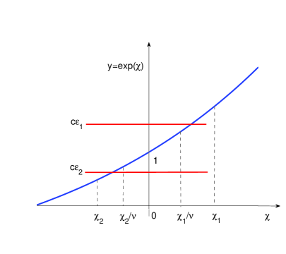
Figure 2.1: Illustration of the improved weights in (2.17); The positive constant $\vartheta$ can squeeze the weights $\frac{1}{c}\exp(\frac{\hat{F}(\theta)-F(\theta)}{\vartheta})$ into $[\epsilon_{1},\epsilon_{2}]$, where $c$ is the normalization constant.

By (2.17), we find that the new weights not only keep the original order in (2.16) but also alleviate the degeneracy phenomenon, where one of weights is too close to 1. In other words, a proper selection of $\vartheta$ will decrease the large weight and increase the small weight simultaneously, which can squeeze the weights into the interval $[\epsilon_{1},\epsilon_{2}]$ (see Figure 2.1). In particular, the weight of each sample will be close to $\frac{1}{N_{s}}$ when $\vartheta$ tends to infinity, where $N_{s}$ is the number of samples from the implicit sampling. A simple method for dynamically selecting scale parameters $\vartheta$ is based on effective sample size (ESS) [16], which can be regarded as the size of random samples with the same variance The algorithm is given in Table 3. As a special case of importance sampling, we can compute the ESS of improved implicit sampling according to the following formula [2, 42]

$$\text{ESS}=\frac{1}{\sum_{i=1}^{N}\omega_{i}^{2}},$$ (2.18)

where $\omega_{i}$ is the weight in improved implicit sampling. We first give a preset value $\mathcal{S}$ of the target ESS and the maximum iterations $N_{\vartheta}$. If the ESS is too small, we can increase $\vartheta$ until it reaches the threshold value $\mathcal{S}$.

Table 3: A strategy for selecting scale parameter $\vartheta$

Input: the preset value of $\mathcal{S}$ and the maximum iteration $N_{\vartheta}$;
Output: $\vartheta_{k}$
1. $\bf{Initialize}$ Set $k=0$ and give the initial value $\vartheta_{0}=1$;
2. $\bf{While}$ $k<N_{\vartheta}$
3. Compute ESS by $\rm ESS=\frac{1}{\sum_{i=1}^{N}\omega_{i}^{2}}$;
4. If $\text{ESS}<\mathcal{S}$
Update $\vartheta_{k}=\vartheta_{k}+1$ and set $k=k+1$;
5. $\bf{end}$

We can find that the samples generated by improved implicit sampling are not only independent of each other but can concentrate on the region with high probability. In improved implicit sampling, one can avoid the case where the support of posterior density is too wide and catch some non-Gaussian feature of the posterior simultaneously. Improved implicit sampling shares the merit of importance sampling and implies a high probability region of the posterior by solving a nonlinear algebraic equation. Based on the Gaussian prior and Laplace prior described in section 2.1 and 2.2, the algorithm of the improved implicit sampling is listed in Table 4, where the scale parameter $\nu$ is selected by Table 3.

Table 4: Improved implicit sampling

1. Compute the MAP point $\theta_{MAP}$ by augmented-Tikhonov algorithm or
the iteratively reweighted approach;
2. Compute the Cholesky factorization $L$ of matrix $\mathcal{H}^{-1}$;
3. $\bf{For}$ $1\leqslant i\leqslant N_{s}$
4. Generate samples by $\theta_{i}=\theta_{MAP}+L^{T}\xi_{i}$, where $\xi_{i}\thicksim N(0,\text{I})$;
5. Compute the weights of samples by $\omega_{i}=\exp(\frac{\hat{F}(\theta_{i})-F(\theta_{i})}{\vartheta})$, then normalization;
6. Resampling based on weights;
7. $\bf{end}$

3 Reduced model based on mixed GMsFEM

We will apply the improved implicit sampling to the inverse problems of the multi-term time fractional diffusion equation, which is described as

$$\begin{cases}(\gamma_{1}\cdot{}_{0}D_{t}^{\alpha_{1}}+\gamma_{2}\cdot{}_{0}D_{t}^{\alpha_{2}})u(x,t)-div(k(x)\nabla u(x,t))+q(x)u(x,t)=f(x,t)\ \ \text{in}\ \ \Omega\times(0,T],\\ u(x,0)=0\ \ \text{in}\ \ \Omega,\\ u(x,t)=g(x,t)\ \ \text{on}\ \ \partial\Omega\times(0,T],\end{cases}$$ (3.19)

where $\gamma_{1}$ and $\gamma_{2}$ are some positive constants, and $\alpha_{1},\alpha_{2}\in(0,1)$ are the fractional orders of the derivative in time. Here ${}_{0}D_{t}^{\alpha}u$ refers to the Caputo derivative [25] with respect to $t$, i.e.,

$${}_{0}D_{t}^{\alpha}u=\frac{1}{\Gamma(1-\alpha)}\int_{0}^{t}\frac{\partial u(x,s)}{\partial s}\frac{ds}{(t-s)^{\alpha}},$$ (3.20)

where $\Gamma$ is the Gamma function. In practice, the diffusion field $k(x)$ is heterogeneous and spatially varies in different scales.

In this section, we present a mixed GMsFEM for solving multi-term time fractional multiscale diffusion equation. Following the mixed GMsFEM framework in [12], the main idea of mixed GMsFEM is to divide the computation into offline stage and online stage. It produces a coarsen computational model. For mixed GMsFEM, we first need to construct the snapshot space. Let $E_{i}$ and $e_{j}$ be the coarse grid edge and the find grid edge, respectively (see Figure 3.2). We define

$$\delta_{j}^{i}=\begin{cases}\ 1&\ \ \text{on $e_{j}$},\\ \ 0&\ \ \text{on other fine grid edges on $E_{i}$}.\end{cases}$$ (3.21)

For the local snapshot $\Psi^{i,snap}_{j}:=v_{j}^{i}$, we need to solve the following problem on the coarse neighborhood $\omega_{i}$ associated with the edge $E_{i}$,

$$\begin{cases}k^{-1}v_{j}^{(i)}+\triangledown p_{j}^{i}=0\ \ \ in\ \ \omega_{i},\\ div(v_{j}^{(i)})=\alpha_{j}^{(i)}\ \ \ in\ \ \omega_{i},\\ v_{j}^{(i)}\cdot n_{i}=0\ \ \ on\ \ \ \partial\omega_{i},\end{cases}$$ (3.22)

where $n_{i}$ denotes the outward unit-normal vector on $\partial\omega_{i}$ and the constant $\alpha_{j}^{(i)}$ satisfies the compatibility condition $\int_{K_{l}}\alpha_{j}^{(i)}=\int_{E_{i}}\delta_{j}^{i}$. We note that the coarse edge $E_{i}$ can be represented by a collection of the fine grid edges $e_{j}$, i.e., $E_{i}=\sum_{j=1}^{J_{i}}e_{j}$, where $J_{i}$ is the total number of the fine grid edges on $E_{i}$, see Figure 3.2.

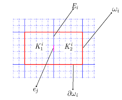
Figure 3.2: An illustration of a neighborhood $\omega_{i}=K_{1}^{i}\cup K_{2}^{i}$ based on a coarse grid edge $E_{i}$.

Then we define the snapshot space $V_{snap}$ by

$$V_{snap}={\rm span}\{\Psi^{i,snap}_{j}:\ \ \ 1\leq j\leq J_{i},\ \ \ 1\leq i\leq N_{e}\}.$$

Let $M_{snap}=\sum_{i=1}^{N_{e}}J_{i}$. Then the snapshot space can be represented as

$$V_{snap}={\rm span}\{\Psi^{snap}_{j}:\ \ \ 1\leq j\leq M_{snap}\}.$$

Therefore we can define a matrix as

$$R_{snap}=[\psi_{1}^{snap},\cdots,\psi_{M_{snap}}^{snap}].$$

To capture the important information in the snapshot space and reduce the dimension of the snapshot space, we consider the local spectral problem: find the eigen-pair $\{\lambda\}$ such that

$$a_{i}(v,w)=\lambda s_{i}(v,w)\ \ \ \forall w\in V_{snap}^{i},$$ (3.23)

where $a_{i}(v,w)$ and $s_{i}(v,w)$ are defined as following

$$\begin{cases}a_{i}(v,w)=\int_{E_{i}}k^{-1}(v\cdot m_{i})(w\cdot m_{i})\\ s_{i}(v,w)=\int_{\omega_{i}}k^{-1}v\cdot w+\int_{\omega_{i}}div(v)div(w).\end{cases}$$

Then we can obtain a matrix representation as

$$A_{snap}^{(i)}Z_{k}^{i}=\lambda_{k}^{i}S_{snap}^{(i)}Z_{k}^{i},$$

where

$$A_{snap}^{(i)}=R_{snap}^{T}A_{fine}^{i}R_{snap},\ \ S_{snap}^{(i)}=R_{snap}^{T}S_{fine}^{i}R_{snap}.$$

Taking the first $L_{b}$ smallest eigenvalues and the corresponding eigenfunctions, the global offline space can be constructed as

$$V_{H}= \{\Psi_{k}^{i}:\Psi_{k}^{i}=\sum_{j=1}^{J_{i}}Z_{kj}^{i}\Psi_{j}^{i,snap},1\leq k\leq L_{b},1\leq i\leq N_{e}\}.$$

This space will be used to approximate the velocity in mixed GMsFEM. If we represent each $\Psi_{k}^{i}$ by the basis functions supported on fine grid and use a single index notation, then we can obtain the following matrix form

$$R_{\text{off}}=[\psi_{1},\psi_{2},\cdots,\psi_{M_{t}}],$$

where $M_{t}=\sum_{i=1}^{Ne}L_{b}$ denotes the total number of multiscale offline basis functions. Once $R_{\text{off}}$ is computed, it can be repeatedly used for online simulation.

Let $u^{n}=u(.,t_{n})$. In this paper, we use the standard $L_{1}$ method [26] to approximate the Caputo derivative by

$${}_{0}D_{t}^{\alpha}u^{n}=\frac{1}{(\Delta t)^{\alpha}\Gamma(2-\alpha)}\sum_{k=1}^{n}(u^{k}-u^{k-1})\times[(n+1-k)^{1-\alpha}-(n-k)^{1-\alpha}],$$ (3.24)

where $0=t_{0}<t_{1}<\cdots<t_{M}=T,\ t_{n}=n\triangle t$. Let $\eta=-k(x)\nabla u$, and $Q_{H}$ and $Q_{h}$ be the space of piecewise constant functions with respect to the coarse grid and fine grid, respectively. Then we can obtain the weak formulation for (3.19),

$$\begin{cases}\int_{\Omega}k^{-1}(x)\eta\cdot v-\int_{\Omega}div(v)u=-\int_{\partial\Omega}g(x,t)v\cdot n,\ \ \forall v\in V_{H}\\ \int_{\Omega}((\gamma_{1}\cdot{}_{0}D_{t}^{\alpha_{1}}+\gamma_{2}\cdot{}_{0}D_{t}^{\alpha_{2}}))u\cdot p+\int_{\Omega}div(\eta)\cdot p+\int_{\Omega}q(x)u\cdot p=\int_{\Omega}f(x,t)p,\ \ \forall p\in Q_{H}.\end{cases}$$

Suppose that $\eta^{n}=\sum_{i=1}^{M_{t}}\sigma_{i}^{n}\psi_{i}$ and $u^{n}=\sum_{k=1}^{J}\beta_{k}^{n}\phi_{k}$, where $\{\phi_{k}\}_{k=1}^{J}\subseteq Q_{H}$.

Let $s_{i}=(\triangle t)^{\alpha_{i}}\Gamma(2-\alpha_{i})\ (i=1,2)$, $s=\frac{s_{1}s_{2}}{\gamma_{1}s_{2}+\gamma_{2}s_{2}}$ and

$$b_{n}=\sum_{i=1}^{2}[n^{1-\alpha_{i}}-(n-1)^{1-\alpha_{i}}]\cdot\frac{\gamma_{i}s_{i+1}}{\gamma_{1}s_{2}+\gamma_{2}s_{1}},\ \ 1\leqslant n\leqslant M,$$

$$c_{k}=\sum_{i=1}^{2}[2k^{1-\alpha_{i}}-(k+1)^{1-\alpha_{i}}-(k-1)^{1-\alpha_{i}}]\cdot\frac{\gamma_{i}s_{i+1}}{\gamma_{1}s_{2}+\gamma_{2}s_{1}},\ \ 1\leqslant k\leqslant M-1,$$

where $s_{3}=s_{1}$. Then the above weak formulation can be transformed into the following matrix form,

$$n=1,\ \ \begin{pmatrix}A&B\\ sB^{T}&C+sD\end{pmatrix}\begin{pmatrix}\sigma^{1}\\ \beta^{1}\end{pmatrix}=\begin{pmatrix}G(:,1)\\ sF(:,1)+b_{1}C\beta^{0}\end{pmatrix},$$

$$n\geq 2,\ \ \begin{pmatrix}A&B\\ sB^{T}&C+sD\end{pmatrix}\begin{pmatrix}\sigma^{n}\\ \beta^{n}\end{pmatrix}=\begin{pmatrix}G(:,n)\\ sF(:,n)+C[c_{1}\beta^{n-1}+c_{2}\beta^{n-2}+\cdots+c_{n-1}\beta^{1}]+b_{n}\beta^{0}\end{pmatrix},$$

where the matrices $A,B,C,D$ and $F,G$ are the corresponding stiffness matrix, mass matrix and load vectors with respect to the multiscale basis functions. If we denote the analogous fine scale matrices by subscript $(\cdot)_{f}$ in the fine grid basis functions, then we can obtain the following relationship between coarse-grid system and fine-grid system,

$$A=R_{\text{off}}^{\prime}A_{f}R_{\text{off}},\ \ \ B=R_{\text{off}}^{\prime}B_{f}B_{\text{off}},\ \ \ C=G_{\text{off}}C_{f}G_{\text{off}}^{\prime}$$ (3.25)

$$D=G_{\text{off}}D_{f}G_{\text{off}}^{\prime},\ \ G=R_{\text{off}}^{\prime}G_{f},\ \ \ \ \ \ \ \ \ F=G_{\text{off}}F_{f}.$$

Here $G_{\text{off}}$ is the restriction operator from $Q_{H}$ to $Q_{h}$. The fine-scale solution and the coarse-scale solution are connected through the matrix $R_{off}$. From (3.25), we can see that the size of matrix $A$ is $M_{t}\times M_{t}$, which is much smaller than $A_{f}\in\mathbb{R}^{N_{h}\times N_{h}}(M_{t}\ll N_{h})$. This shows the multiscale model reduction in terms of algebraic system.

4 Numerical results

In this section, we present a few numerical experiments to identify the unknown parameters in the muti-term time fractional diffusion equations to evaluate the performance of the improved implicit sampling. The mixed GMsFEM is used to build a surrogate model for the multiscale diffusion models to speed up sampling posterior. In subsection 4.1, we identify the multi-term time fractional derivative orders simultaneously. In subsection 4.2, we recover the diffusion coefficient $k(x)$ based on the Gaussian prior when the two occasions occur: known fractional derivatives and unknown fractional derivatives. In subsection 4.3, the reaction coefficient $q(x)$ is estimated based on Laplace prior.

For the numerical examples, we set the spatial domain $\Omega=[0,1]\times[0,1]$ and the final time $T=1$. Measurement data are generated by the fine grid FEM with time step $\Delta t=0.02$, and the noise level is set to be $\sigma=0.01$. The step size to compute the sensitivity matrix $\bar{H}$ using the difference method is equal to $0.5$.

4.1 Inversion for multi-term time fractional derivative orders

In this subsection, our objective is to identify the multi-term time fractional derivatives in model (3.20), where Dirichlet boundary condition $g(x,t)\equiv 1$ on the four boundary sides, the source term $f(x,t)=10$ and the reaction coefficient $q(x)=1$. The positive constants $\gamma_{1}=0.2$ and $\gamma_{2}=0.8$. The forward model is discretized on a $80\times 80$ uniform fine grid, and we set the coarse grid $8\times 8$ for mixed GMsFEM computation. We consider permeability field $k(x)$ as heterogeneous media illustrated in Figure 4.3 (a). We take $n=240$ Neumann observations on the left and right sides at $t=0.4$ and $t=1$. The reference fractional derivative orders are given as $\alpha_{1}=0.3$ and $\alpha_{2}=0.6$. In the example, the fractional orders are restricted in the interval $(0,1)$ (subdiffusion). To this end, we take a transform [21] as following

$$h(x)=\frac{1}{2}+\frac{1}{\pi}\arctan(x),\ x\in\mathbb{R}.$$

By the transformation, it can make the fractional orders lie in the interval $(0,1)$. We impose a Guassian prior for the unknown parameter vector $[\alpha_{1},\alpha_{2}]$ under the framework of hierarchical Bayesian and the variance $\lambda$ of the Gaussian prior is unknown and regarded as the hyper-parameter. Since the dimension of unknown parameters is relatively low, it is appropriate to set $\vartheta=1$ in this example. The initial guess for $(\alpha_{1},\alpha_{2})$ is given by $(0.5,0.5)$ to compute the MAP point by augmented-Tikhonov algorithm described in Table 1. In the example, the approximated posterior $\tilde{p}(\theta|d)$ refers to the posterior obtained by using mixed GMsFEM and the reference posterior $p(\theta|d)$ is obtained by mixed FEM in the sampling process. To illustrate the convergence of KL divergence $D_{KL}(\tilde{p}(\theta|d)||p(\theta|d))$ [17, 21], we plot the KL curve with respect to the number of multiscale basis functions $L_{b}$ by using 5000 samples generated by improved implicit sampling in Figure 4.3 (b). From this figure, it can be found that the $D_{KL}$ substantially decreases as the number of multiscale basis functions increases. In particular, we also list the CPU time in improved implicit sampling by using mixed GMsFEM and mixed FEM in Table 5. From this table, it can be seen that the CPU time decreases significantly when mixed GMsFEM is applied in the improved implicit sampling.

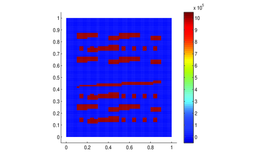
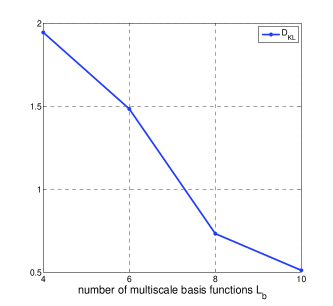
Figure 4.3: (a) The spatial distribution of permeability field; (b) KL divergence between the approximate posterior density $\tilde{p}(\theta|d)$ and reference posterior density $p(\theta|d)$ with respect to the number of multiscale basis funcitons $L_{b}$.

$L_{b}$	4	6	8	10
$t_{off}$	$2.2472s$	$2.3359s$	$2.3870s$	$2.2800s$
$t_{on}$	$3.2088\times 10^{3}s$	$7.0975\times 10^{3}s$	$1.2994\times 10^{4}s$	$2.0652\times 10^{4}s$
$t_{f}$	$2.7453\times 10^{4}s$

Table 5: Comparison of CPU time of improved implicit sampling by using mixed FEM and mixed GMsFEM with respect to the number of multiscale basis functions $L_{b}$. $t_{off}$ and $t_{on}$ are the offline time and online time by using mixed GMsFEM respectively and $t_{f}$ is the total time by using mixed FEM.

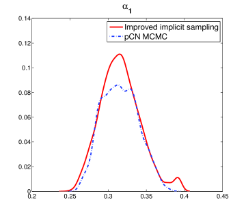
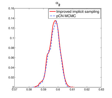
Figure 4.4: The posterior marginal distribution for $\alpha_{1}$ (left) and $\alpha_{2}$ (right) by improved implicit sampling and pCN MCMC method.

In order to compare the performance by using the improved implicit sampling and MCMC sampling, we also use pCN MCMC method [19, 41] to solve the inverse problem. We select $L_{b}=6$ multiscale basis functions at each coarse block to construct the offline space. The tuning parameter in pCN MCMC method is set at $0.05$ with an acceptance probability $30.22\%$ to make the chain efficiently explore the parameter space. The number of samples used in these methods is 5000. The first 1000 steps of the pCN MCMC samples are taken out as the burn-in period and the remaining 4000 samples are used to compute the corresponding statistical quantities. In Figure 4.4, we plot the posterior marginal distribution of the fractional orders by improved implicit sampling and pCN MCMC method, respectively. From this figure, we can see that the posterior marginal distribution of $\alpha_{2}$ produced by the two methods are similar to each other. While for $\alpha_{1}$, it seems that the samples generated by improved implicit sampling have the ability of focusing on the region with high probability than pCN MCMC method, this is because the weights in improved implicit sampling can make the samples be close to the MAP point. By the support of these curves, it can be seen that the uncertainty of $\alpha_{1}$ is larger than that of $\alpha_{2}$. Furthermore, in order to explore the correlation between the two parameters, we present the matrix plot in Figure 4.5. It is clearly to see that the two parameters are strongly negatively correlated.

Next, in order to compare the sampling performance of these two methods, we calculate the effective sample size (ESS). Based on (2.18), we can compute the ESS in improved implicit sampling. There are more than 1712 effective samples in 5000 samples, which is sufficient to verify the validity of improved implicit sampling. In Table 6, we also show the posterior marginal mean and standard deviation of these two methods, both of which give almost the same results. However, the above formula could not be applied to calculating the ESS for MCMC [43]. Alternatively, we adopt the following formula to do some qualitative analysis, i.e.,

$$\text{ESS}=\frac{N_{s}}{\bar{\rho}},$$ (4.26)

where $N_{s}$ is the total number of samples and $\bar{\rho}$ is the averaged integrated auto-correlation time (IACT). For a model with $m$ unknown parameters, IACT $\bar{\rho}$ can be calculated by

$$\bar{\rho}=\frac{1}{m}\sum_{i=1}^{m}(1+2\sum_{k=1}^{\infty}\rho_{k}),$$

where $\rho_{k}$ is the auto-correlation function (ACF) at lag $k$. For a time series $M_{t}$ with mean $\mu_{0}$ and variance $\sigma_{0}^{2}$, $\rho_{k}$ is defined as

$$\rho_{k}=\frac{E[(M_{t}-\mu_{0})^{T}(M_{t+k}-\mu_{0})]}{\sigma_{0}^{2}}.$$

The difference between ESS and the actual sample size is due to the large autocorrelation structure imposed by the MCMC method. In Figure 4.6, we plot the ACF of these two methods. We can see that the ACF of improved impilcit sampling gets closer to 0 as the lag increases. However, it can be seen that the ACF of MCMC method is much larger than that of improved implicit sampling and has no convergence tendency. The figure implies that the ESS of MCMC method is much smaller than improved implicit sampling based on (4.26), though the exact number of the ESS of MCMC method is not sure.

The observations and the actual model response are plotted in Figure 4.7. To construct $95\%$ credible and prediction intervals for model response at $u(0,y;0.4)$ and $u(1,y;0.4)$, we use $5000$ samples to produce realizations of the model. For $u(0,y;0.4)$, we note that the uncertainty focus on the region $[0.3,0.5]$, which is mainly due to the Dirichlet boundary condition imposed in the forward model. It can be also seen from these two figures that most of observations lie in the predictive interval. This implies that the improved implicit sampling properly describes the uncertainty propagation for the model.

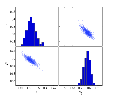
Figure 4.5: The matrix plot for $(\alpha_{1},\alpha_{2})$ by improved implicit sampling.

	Improved implicit sampling	MCMC method
Mean	(0.3160, 0.5974)	(0.3155, 0.5974)
Standard deviation	(0.0262, 0.0038)	(0.0235, 0.0036)

Table 6: The posterior marginal mean, standard derivation for $[\alpha_{1},\alpha_{2}]$ of improved implicit sampling and pCN MCMC method.

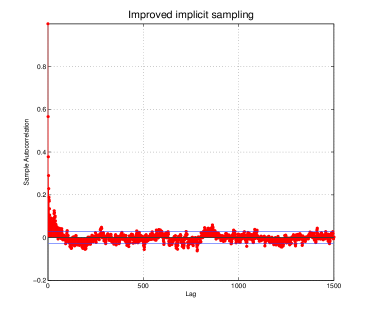
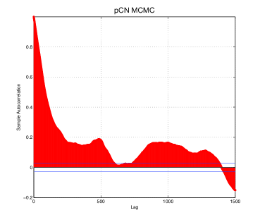
Figure 4.6: The ACF of $\alpha_{1}$ for improved implicit sampling (left) and pCN MCMC method (right).

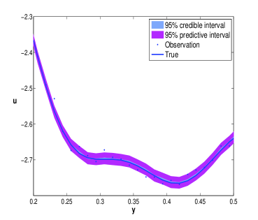
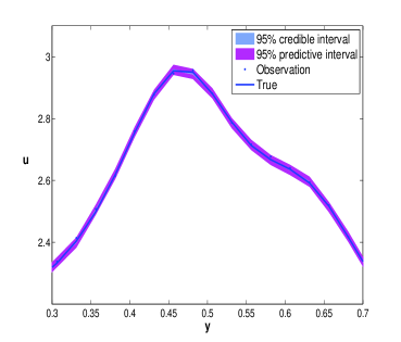
Figure 4.7: Data, true, and $95\%$ credible interval and prediction interval by improved implicit sampling for $u(0,y;0.4)$ (left) and $u(1,y;0.4)$ (right).

4.2 Inversion for diffusion coefficient

In this subsection, we apply the improved implicit sampling to identify the diffusion coefficient $k(x)$ in model (3.19). Assume that $\gamma_{1}=\gamma_{2}=1$ and the fractional orders $\alpha_{1}=0.3,\ \alpha_{2}=0.6$ are fixed. The reaction coefficient $q(x)=1$ is fixed in this example. For this example, we set the source term $f=10$ and the Dirichlet boundary condition $g=1$. In order to reduce the dimension of the grid-based unknown input $k(x)$, we regard it as a random field $k(x,\varrho)$ and assume the log permeability field $\log[k(x,\varrho)]$ can be represented by the Karhunen-Lo$\grave{e}$ve expansion [38]. In particular, we consider a correlated second-order Guassian random field $k(x,\varrho)$ [38] defined for $x\in\Omega$ with the expectation $\text{E}[k(x,\varrho)]$ and covariance function $C(x;y)$. For $k(x,\varrho)$, it can be represented as

$$\log k(x,\varrho)=\text{E}[k(x,\varrho)]+\sum_{j=1}^{\infty}\sqrt{\lambda_{j}}\zeta_{j}(x)v_{j}(\varrho),$$

where $\lambda_{j}$ and $\zeta_{j}$ are the eigenvalues and orthonormal eigenfunctions of the covariance function $C(x;y)$ satisfying

$$\int_{\Omega}C(x;y)\zeta_{j}(y)dy=\lambda_{j}\zeta_{j}(x)$$

for $x\in\Omega$. We note that the random variables $v_{j}(\varrho)$ are centered and uncorrelated. In addition, we assume the covariance function

$$C(x_{1},x_{2};y_{1},y_{2})=\rho^{2}\exp(-\frac{|x_{1}-y_{1}|^{2}}{2l_{1}^{2}}-\frac{|x_{2}-y_{2}|^{2}}{2l_{2}^{2}}).$$

In order to reduce the dimension of the unknown parameters, the truncated expansion based on the decay rate of the eigenvalues $\lambda_{j}$ is usually employed for numerical simulation, which can be expressed as

$$\log k(x,\varrho)=\text{E}[k(x,\varrho)]+\sum_{j=1}^{l}\sqrt{\lambda_{j}}\zeta_{j}(x)v_{j}(\varrho)$$ (4.27)

for $l\ll m$. Finally, one can rewrite (4.27) in a matrix formulation as

$$\log k(x,\varrho)=\Phi\textbf{v}+\kappa,$$

where $\kappa=\text{E}[\theta(x,\varrho)]$ and $\Phi=[\sqrt{\lambda_{1}}\zeta_{1},\cdots,\sqrt{\lambda_{l}}\zeta_{l}]$. As a result, the unknown parameter $\textbf{v}\in\mathbb{R}^{l}$ needs to be estimated under the Bayesian framework.

As a prior information, $\text{E}(\log[k(x,\varrho])$ is illustrated in Figure 4.8. The corresponding parameters in the covariance function are given by $\rho=0.5$, and $l_{1}=l_{2}=0.1$. To reduce the dimensional of the unknown coefficient, we retain the first 12 terms based on the decay of the eigenvalues. The forward model is computed on a uniform $80\times 80$ fine grid and the coarse grid is $5\times 5$ for mixed GMsFEM. We choose $L_{b}=6$ multiscale basis functions to construct the offline space. When we compute the matrix $R_{\text{off}}$, the number of training parameters used in this example is $12$. We choose the whole boundary Neumann data at $t=0.6$ as measurements.

In Figure 4.9, we plot the spatial distribution of the reference, the corresponding posterior mean and the standard deviation in a logarithmic scale by the improved implicit sampling with $5000$ samples. The scale parameter $\vartheta$ is fixed at 1. From these figures, it can be seen that the posterior mean can approximate the reference well. We note that the standard deviation at the center of the physical domain is large. This may be because that only the boundary Neumann data are used to recover the unknown coefficient.

We use augmented-Tikhonov method to compute MAP point. The convergence of the method is shown in Figure 4.10. From Figure 4.10 (a), it can be seen that the relative errors rapidly decrease in the first three iterations. Meanwhile, from Figure 4.10 (c), we can find that the hyper-parameter $\lambda$ exhibits a stable convergence trend after a few iterations, which implies the effectiveness of augmented-Tikhonov method. As we know, the regularization parameter plays a crucial role in inverse problems, and there are a few strategies to select it. In order to compare the hierarchical Bayesian model with discrepancy principle [37], a method of selecting regularization parameters, we plot $\|H(\textbf{v})-d\|^{2}_{2}$ and $n\sigma^{2}$ versus the iterative steps in Figure 4.10 (b). As we expect, $\|H(\textbf{v})-d\|^{2}_{2}$ decreases fast firstly and then becomes stable after the third iterative step. Though the final value of $\|H(\textbf{v})-d\|^{2}_{2}$ is not exactly equal to $n\sigma^{2}$, the regularization parameter $\mu=\lambda\sigma^{2}$ determined by the hierarchical Bayesian model can be also regarded as an approximate solution of the following nonlinear equation

$$\|H(\textbf{v}_{\mu})-d\|^{2}_{2}-n\sigma^{2}=0,$$

which is the practical implementation of discrepancy principle.

To construct $95\%$ credible intervals for the model response, $5000$ model realizations generated by improved implicit sampling are used here. The measurement error is incorporated to construct the prediction intervals. The credible interval and predictive interval, together with the true model response and data, are plotted in Figure 4.11. From this plot, we can see that the synthesized data are almost contained in the prediction intervals. As illustrated in Figure 4.11, the prediction interval gets wider as $y$ increases for $u(0,y;0.6)$ in $[0.1,0.3]$. This is because of the imposed Dirichlet boundary condition.

Next we identify the multi-term time fractional derivative orders and the diffusion field simultaneously. For this simulation, we reset the boundary condition $g=1+x_{1}$ and the source term $f=2x_{1}+2$. The positive constants and the reference multi-term time fractional orders are chosen the same as in Section 4.1. In addition, the reference diffusion field is the same as Figure 4.9 (a). The mesh partition of the forward model is the same as before. Thus we need to recover the unknown parameter $\textbf{v}=[\alpha_{1},\alpha_{2},v_{1},\cdots,v_{12}]\in\mathbb{R}^{14}$ in this case. We first implement the augmented-Tikhonov algorithm to obtain the MAP estimate. Then we use conventional implicit sampling and improved implicit sampling to make comparison. We first compute the weight of each sample generating from the conventional implicit sampling method. In this method, the excessive concentration of weights occurs. That is to say, one weight of the particle is close to $1$ and other particles have no influence since their weights are too small, which will result in a poor representation of the posterior. In order to avoid filter collapse, we adopt the formulation in (2.17) to improve the weights. We note that the weights in the improved implicit sampling obey the formula (2.17) and the weights in the conventional implicit sampling obey the formula (2.16). To show the distribution of the weights for the two implicit sampling methods, we count the number of samples when associated weights lie in the disjoint intervals and list the results in Table 7. Here we set the scale parameter $\vartheta=15$ for the improved implicit sampling. From this table, it can be found that most of the samples have extremely small weights in the conventional implicit sampling, which will cause the ensemble collapse. Thus, the conventional implicit sampling may underestimate the uncertainty of the unknown parameters. But for the improved implicit sampling, we can see that the distribution of weights is relatively flat while it retain the original order. This is a significant improvement. In order to clearly illustrate the effect of the two implicit sampling on the posterior distribution, we plot the marginal posterior histogram of $[\alpha_{1},\alpha_{2},v_{1},v_{7},v_{12}]$ in Figure 4.12. It can be seen that samples are over-concentrate by the conventional implicit sampling and the improved implicit sampling effectively alleviates the situation. This is consistent with the results in Table 7.

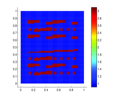
Figure 4.8: The spatial distribution of $\text{E}(\log k(x,\varrho))$.

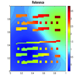
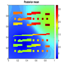
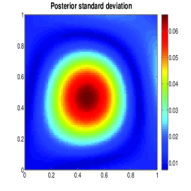
Figure 4.9: The reference solution (left), the posterior mean (middle) and posterior standard deviation (right) of $\log k(x,\varrho)$ by improved implicit sampling.

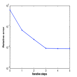
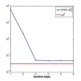
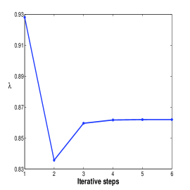
Figure 4.10: Numerical results of augmented-Tikhonov method to compute the MAP point.

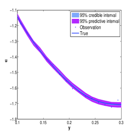
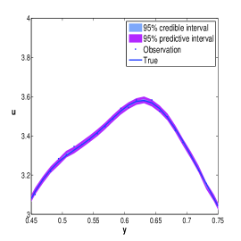
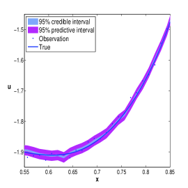
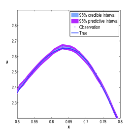
Figure 4.11: Data, true, and $95\%$ credible interval and prediction interval by improved implicit sampling for (a) $u(0,y;0.6)$, (b) $u(1,y;0.6)$, (c) $u(x,0;0.6)$, (d) $u(x,1;0.6)$.

Method	Interval
	[0, $10^{-6}$)	[$10^{-6}$, $10^{-5}$)	[$10^{-5}$,$10^{-4}$)	[$10^{-4}$,$10^{-3}$)	[$10^{-3}$,$10^{-2}$)	[$10^{-2}$,$10^{-1}$)	[$10^{-1}$,1]
I-IS	3004	423	593	750	219	11	0
C-IS	4993	3	1	1	0	1	1

Table 7: The weights distribution for improved implicit sampling (I-IS) and conventional implicit sampling (C-IS)

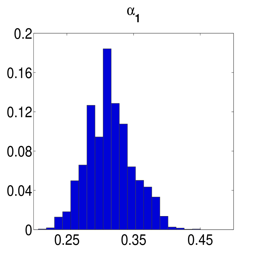
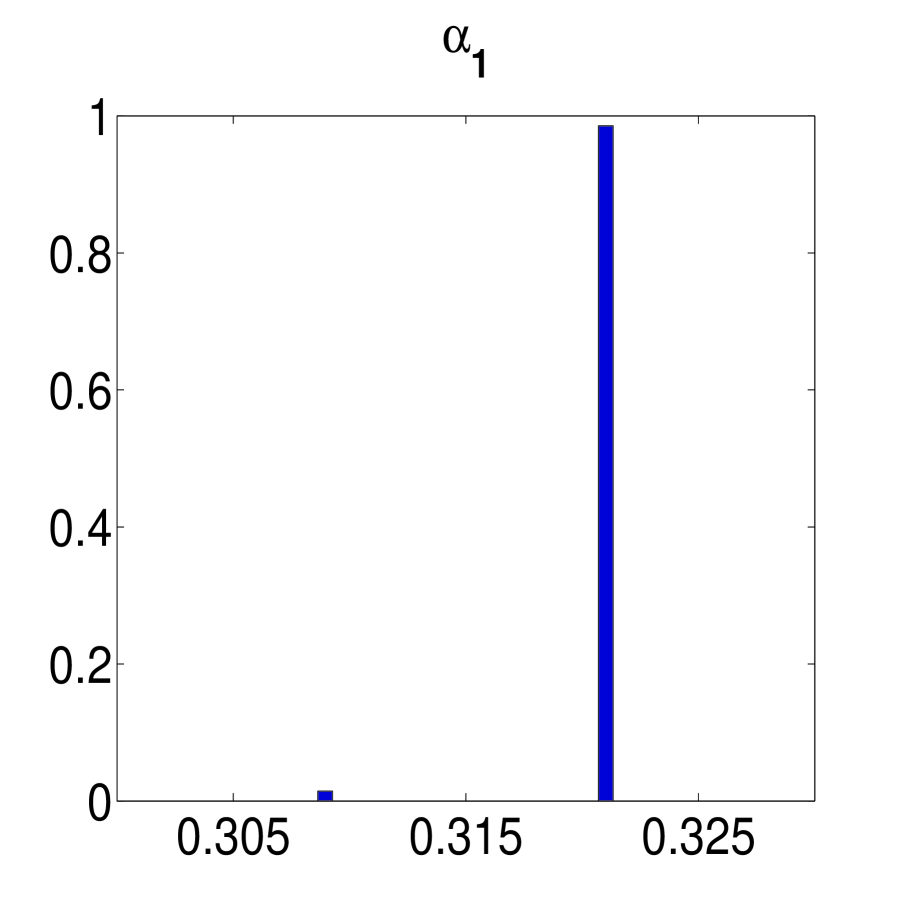
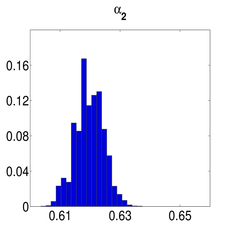
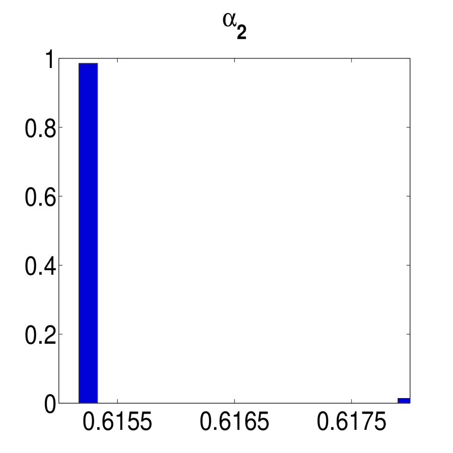
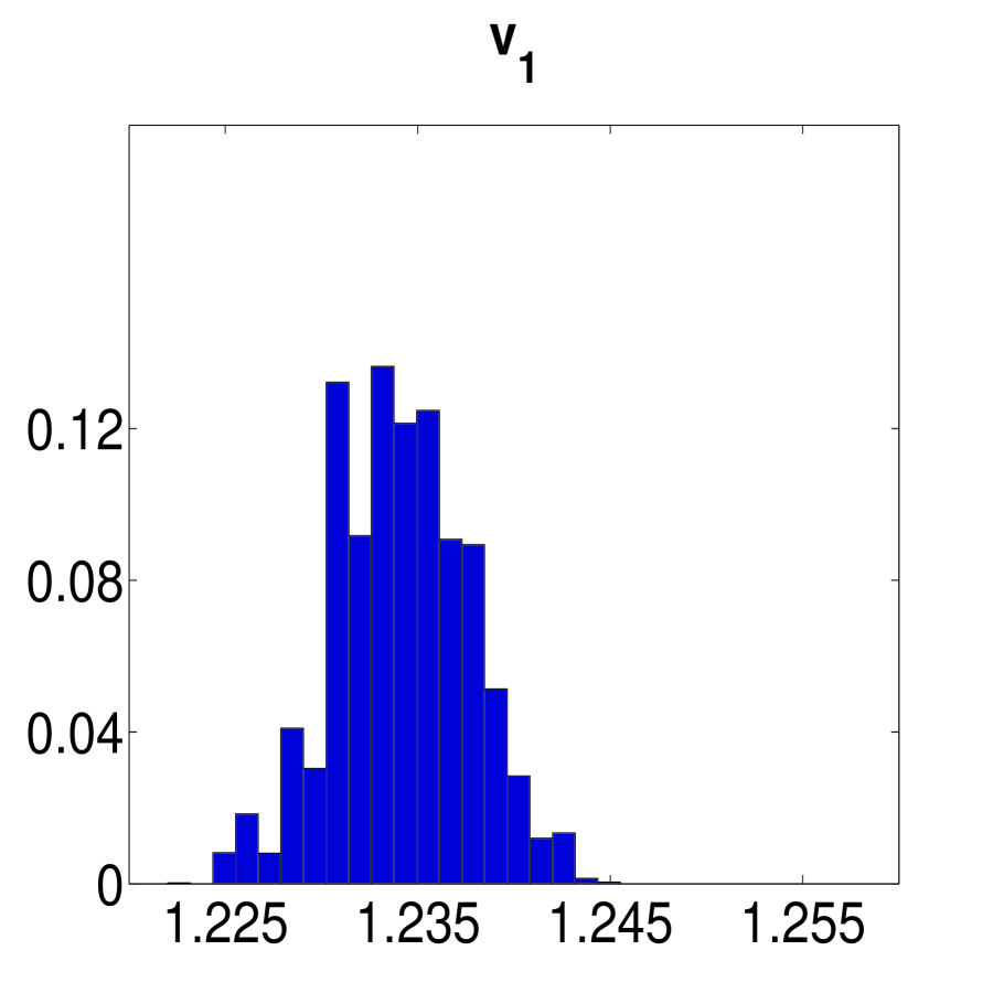
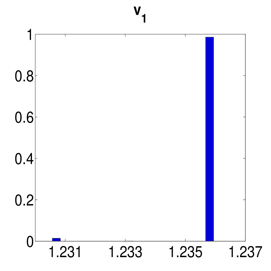
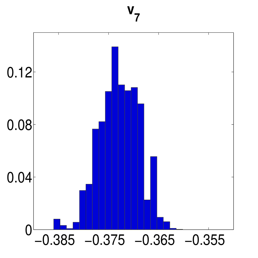
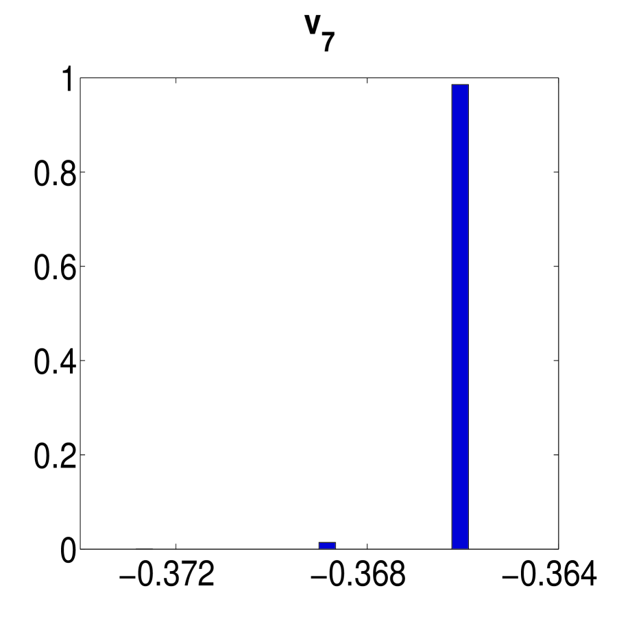
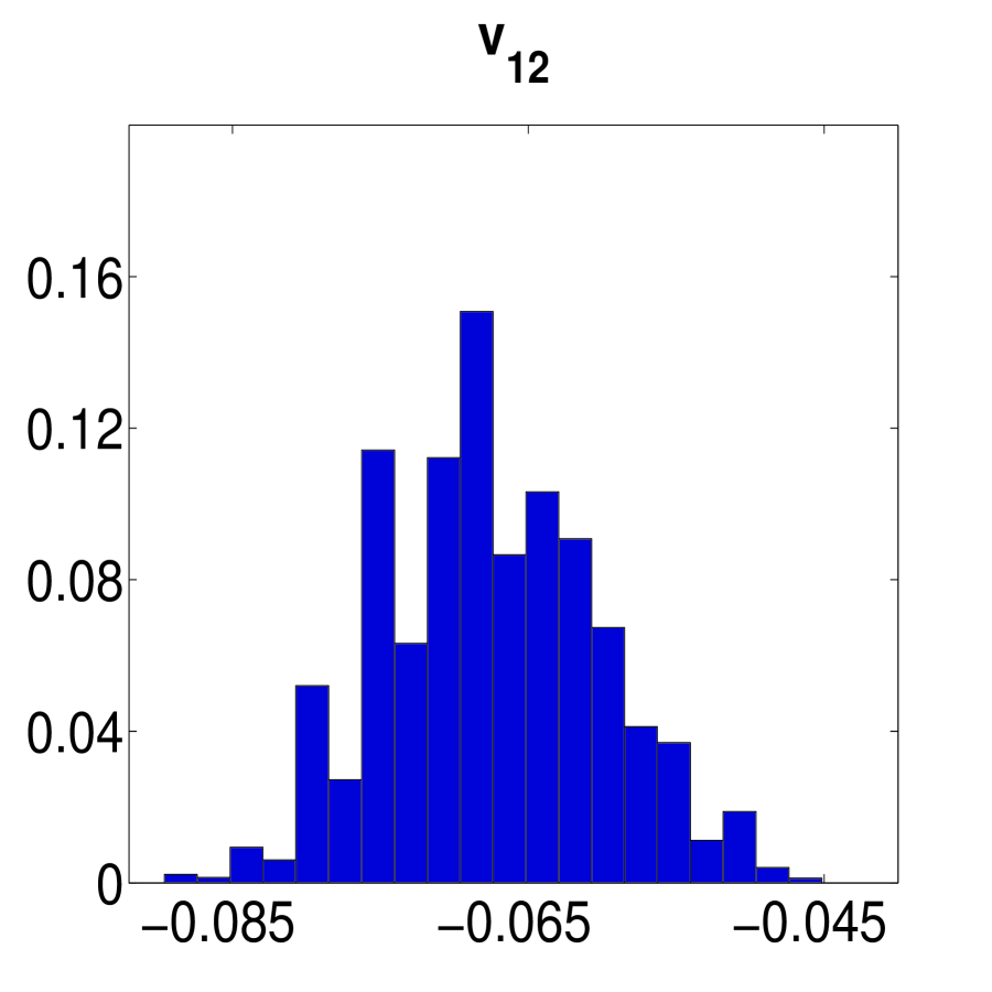
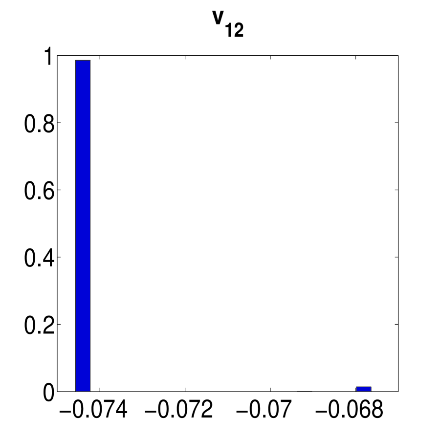
Figure 4.12: The histogram of marginal posterior by improved implicit sampling (the first row) and conventional implicit sampling (the second row) for $[\alpha_{1},\alpha_{2},v_{1},v_{7},v_{12}]$.

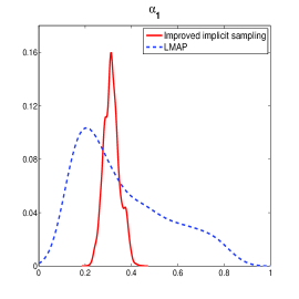
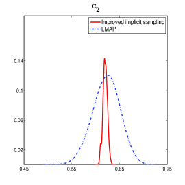
Figure 4.13: The posterior marginal distribution for $\alpha_{1}$ (left) and $\alpha_{2}$ (right) by improved implicit sampling and LMAP.

	Skewness	Kurtosis
Improved implicit sampling	(0.2841, -0.0662)	(-0.0392, 0.0230)
LMAP	(0.7403, -0.1804)	(-0.5048, -0.1120)

Table 8: The skewness and kurtosis of $(\alpha_{1},\alpha_{2})$ by improved implicit sampling and LMAP.

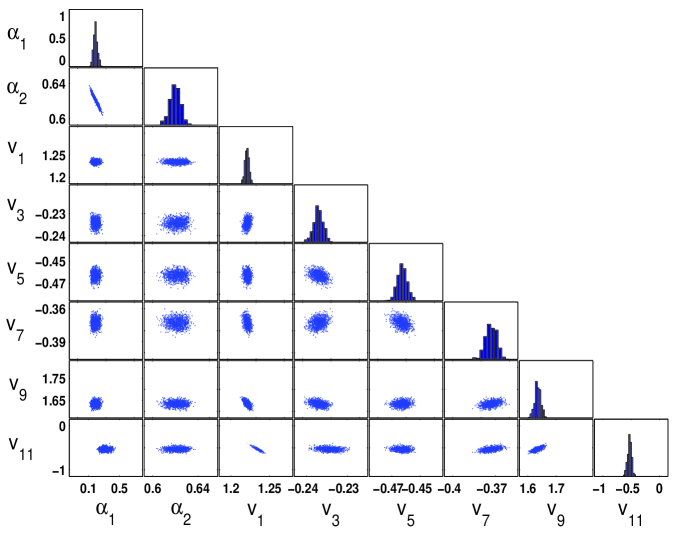
Figure 4.14: The matrix plot for $[\alpha_{1},\alpha_{2},v_{1},v_{3},\cdots,v_{11}]$ by improved implicit sampling.

Finally we make a comparison between improved implicit sampling and LMAP. Figure 4.13 plots the marginal posterior for $\alpha_{1}$ and $\alpha_{2}$ using these two approaches, which illustrates that samples by improved implicit sampling are more concentrated on the region near MAP point than LMAP. To characterize the marginal posterior distribution of $(\alpha_{1},\alpha_{2})$, we list the skewness and kurtosis of the two parameters based on samples by the improved implicit sampling and LMAP method in Table 8. We find that the skewness of $\alpha_{1}$ produced by LMAP method is positive and it implies that the heavy tail is on the right, which is consistent with Figure 4.13 (a). To describe the correlation among these parameters, the matrix plot for $[\alpha_{1},\alpha_{2},v_{1},v_{3},\cdots,v_{11}]$ is shown in Figure 4.14. It is observed from the pairwise joint sample plots in Figure 4.14 that the multi-term fractional orders $\alpha_{1}$ and $\alpha_{2}$ are clearly negatively correlated, which is consistent with section 4.1. We can also conclude that the fractional orders are almost independent of all the parameters in the diffusion field. The parameters in the diffusion field are almost independent except for a small correlation between $v_{1}$ and $v_{11}$.

4.3 Inversion for reaction coefficient

In this subsection, we aim at recovering the reaction coefficient $q(x)$. The truth of $q(x)$ is depicted in Figure 4.15 (a). As illustrated in Subsection 4.2, we assume that the unknown reaction field $q(x,\varrho)$ can be parameterized by Karhunen-Lo$\grave{e}$ve expansion. For the covariance function of $\log q(x,\varrho)$, we set $l_{1}=l_{2}=0.03$, $\rho=1$ and $\kappa=1$. Here, the first 34 terms are truncated for the parametrization. The forward model is defined on $50\times 50$ uniform fine grid, and mixed GMsFEM model is implemented on $5\times 5$ coarse grid. The number of local multiscale basis functions is set to $5$. We choose the source term $f=10$ and the Dirichlet boundary condition $g=1-x_{1}$. The measurements are taken at $t=0.6$ from the whole boundary Neumann data, whose distribution is shown in Figure 4.15 (b).

In this subsection, we attempt to use sparse prior information to recover the unknown $q(x,\varrho)$. Assume that the regularization parameter $\mu=0.005$ is fixed. In order to illustrate the performance of the iteratively reweighted approach, we plot the reconstruction results in Figure 4.16. By Figure 4.16, after five iterations, the inversion solution can effectively capture the major feature of the truth profile although the measurement data are only collected on the boundary.

In order to compute the statistical information, $5000$ samples are produced by implicit sampling. However, some of weights are close to $1$ if we use the conventional implicit sampling. To avoid this degenerative situation, we choose the scale parameter $\vartheta$ acting as the relaxation factor for improved implicit sampling. We can select the parameter $\vartheta$ dynamically based on the ESS in (2.18). In this example, we set $\vartheta=10$ to ensure the ESS to be more than $1000$. We list the distribution of weights corresponding to samples by improved implicit sampling and conventional implicit sampling in Table 9. It is obvious that the improved implicit sampling gives much better distribution of weights of samples than the conventional implicit sampling. The histogram of the marginal posterior by the two implicit sampling methods for the parameter vector $[v_{1},v_{8},v_{15},v_{22},v_{30}]$ are plotted in Figure 4.17, which agrees with the results in Table 9. The posterior mean and standard derivation by the improved implicit sampling are plotted in Figure 4.18. This figure illustrates that the uncertainty mainly occurs around the region with large jump.

The $95\%$ credible intervals for model response at the measurement locations from the $5000$ realizations of the model are plotted in Figure 4.19. The prediction intervals are built by incorporating the measurement error $\sigma$ and showed in Figure 4.19, which shows most measurement data lies in the $95\%$ prediction interval.

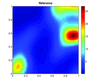
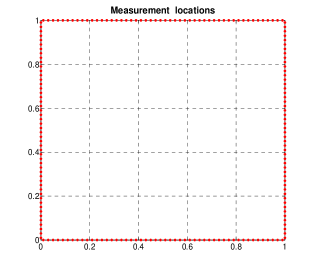
Figure 4.15: The truth profile of $q(x)$ and the measurement distribution for Subsection 4.3.

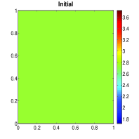
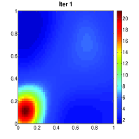
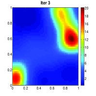
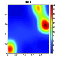
Figure 4.16: The initial guess (a) and the reconstruction results (b-d) for $q(x,\varrho)$ in the $1$-st, $3$-rd and $5$-th iteration.

Method	Interval
	[0, $10^{-6}$)	[$10^{-6}$, $10^{-5}$)	[$10^{-5}$,$10^{-4}$)	[$10^{-4}$,$10^{-3}$)	[$10^{-3}$,$10^{-2}$)	[$10^{-2}$,$10^{-1}$)	[$10^{-1}$,1]
I-IS	2	186	2412	2262	138	0	0
C-IS	4940	23	13	14	6	3	1

Table 9: The distribution of the weights for improved implicit sampling (I-IS) and conventional implicit sampling (C-IS).

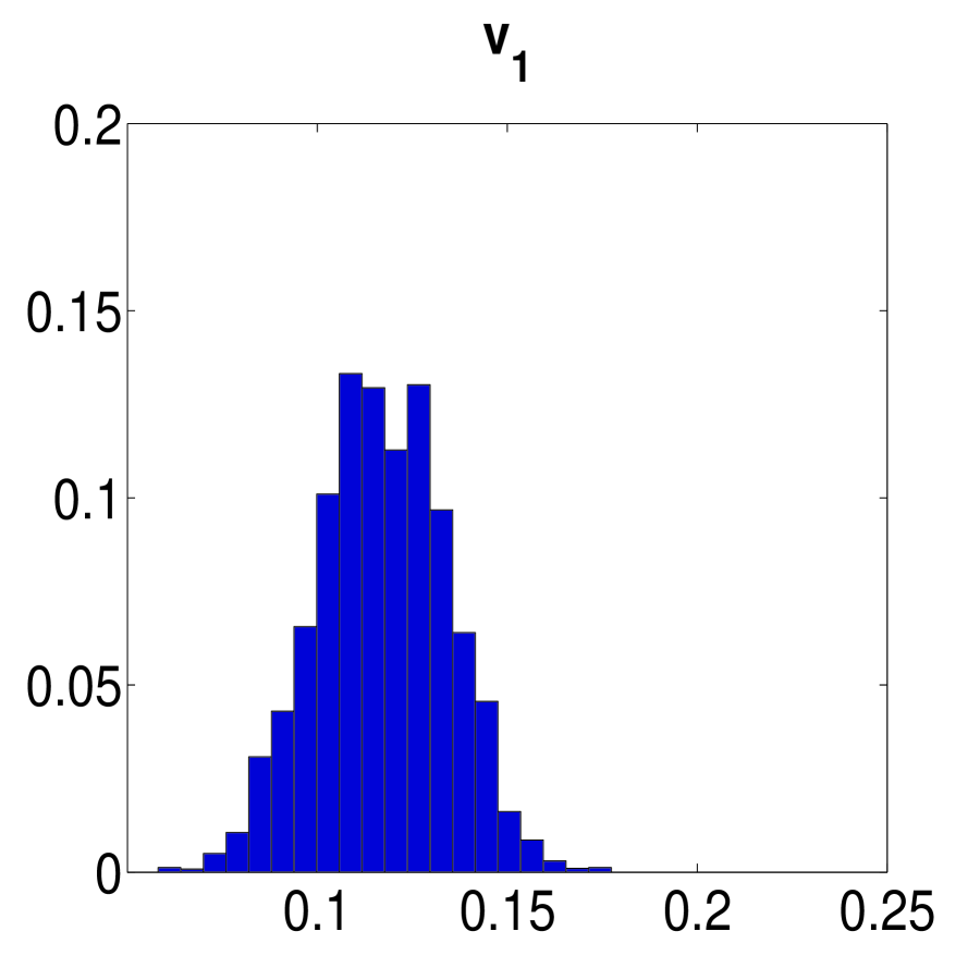
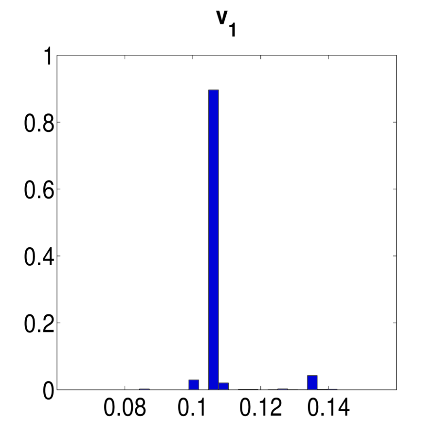
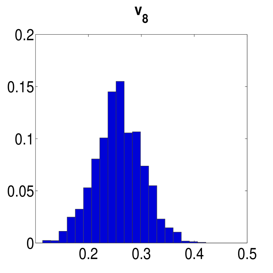
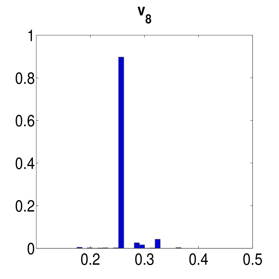
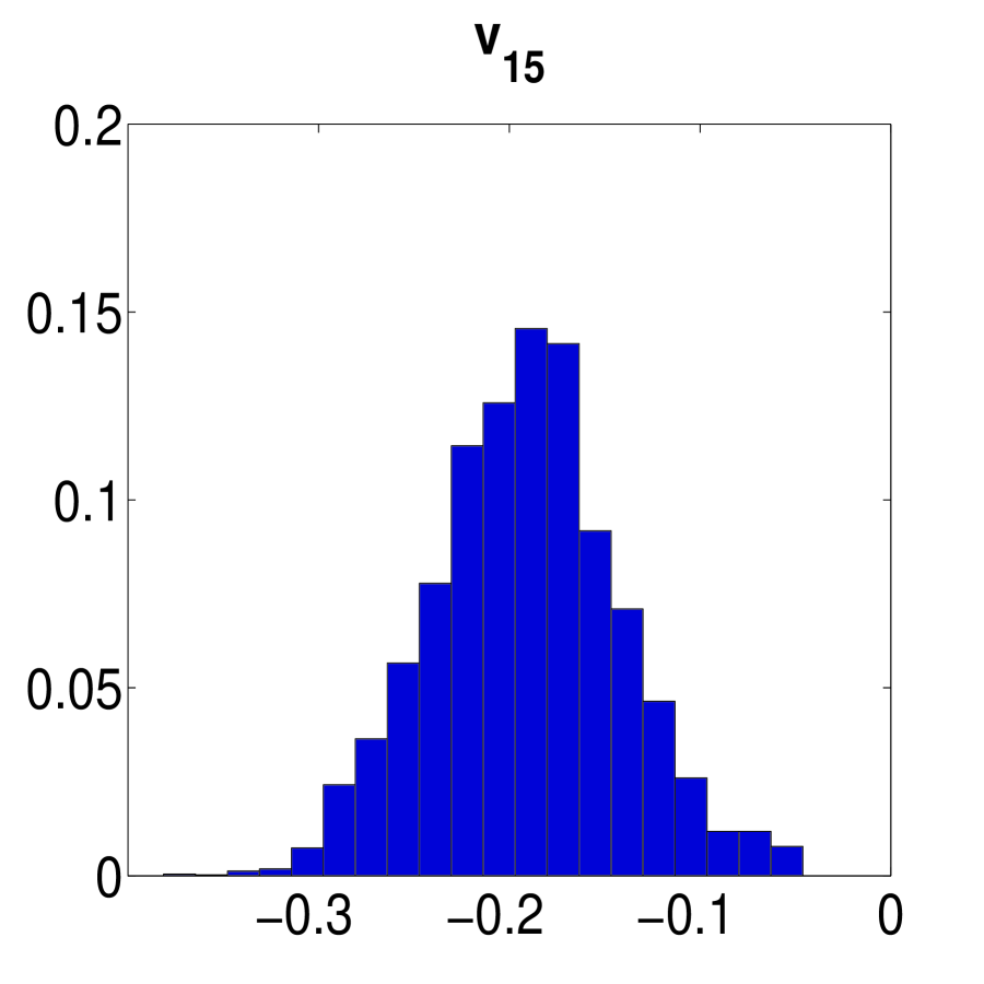
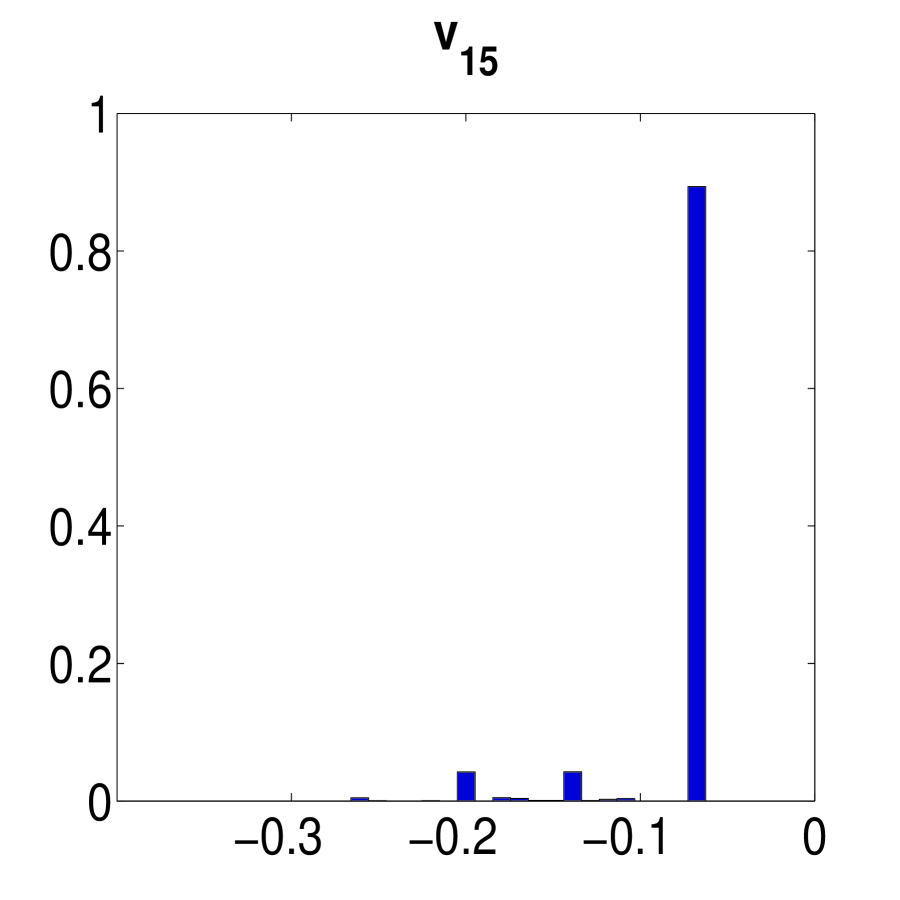
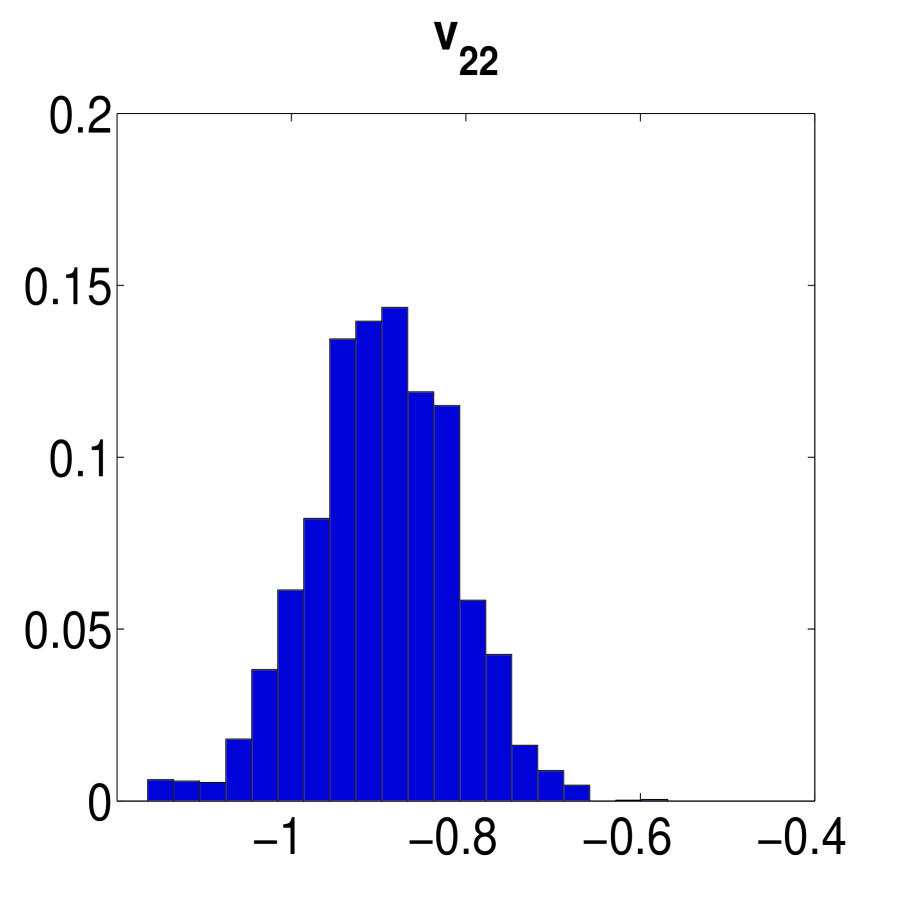
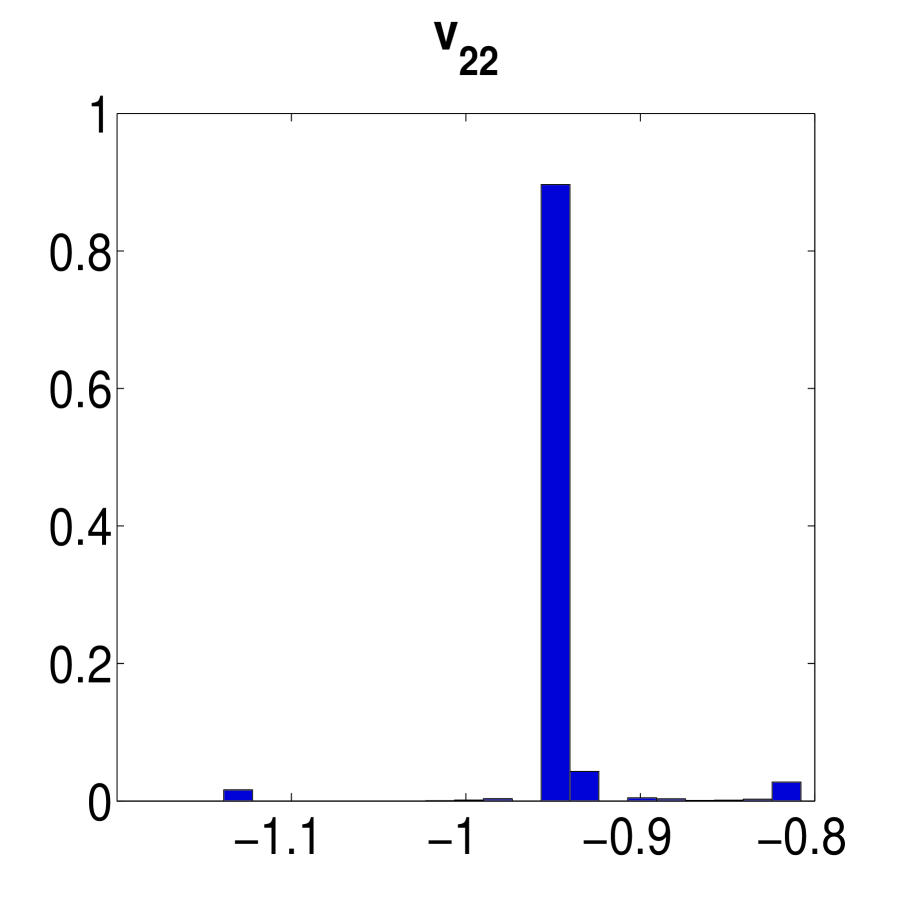
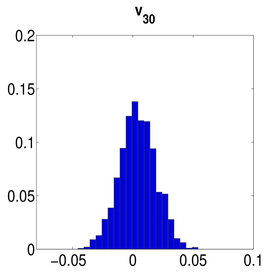
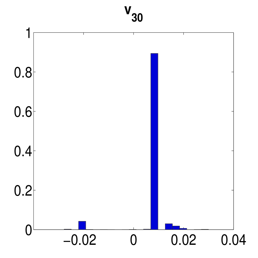
Figure 4.17: The histogram of marginal posterior by improved implicit sampling (the first row) and conventional implicit sampling (the second row) for $[v_{1},v_{8},v_{15},v_{22},v_{30}]$.

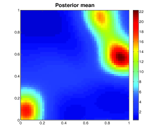
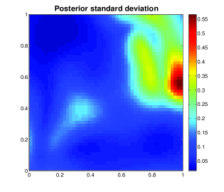
Figure 4.18: The posterior mean (left) and posterior standard deviation (right) of $q(x,\varrho)$ by improved implicit sampling.

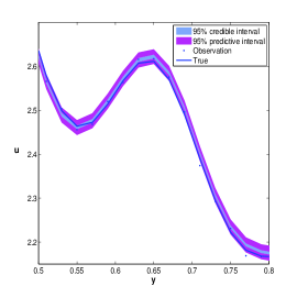
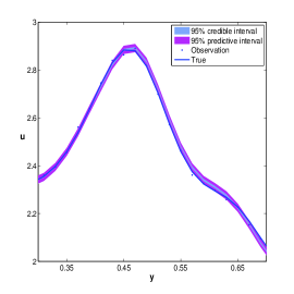
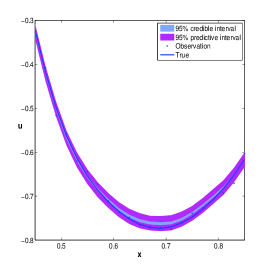
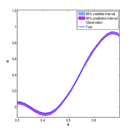
Figure 4.19: Data, true, and $95\%$ credible interval and prediction interval by improved implicit sampling for (a) $u(0,y;0.6)$, (b) $u(1,y;0.6)$, (c) $u(x,0;0.6)$, (d) $u(x,1;0.6)$.

5 Conclusions

In this work, we presented an improved implicit sampling method for Bayesian inverse problems. The approach generated independent samples around the region with high probability, i.e. near the MAP point. However, the weights of conventional implicit sampling may cause excessive concentration of samples and lead to ensemble collapse, which would result in the poor estimation of the posterior. In order to avoid this issue, we proposed a new weight formulation for implicit sampling. For more practical applications, we considered the improved implicit sampling for hierarchical Bayesian models. As an application, we focused on the multi-term time fractional multiscale diffusion equations. To effectively capture the multiscale and heterogeneity feature of the diffusion field, we presented a mixed GMsFEM to build a reduced model and speed up the Bayesian inversion. Some comparison were carried out among improved implicit sampling,conventional sampling and LMAP method by a few numerical examples. We found that the proposed improved implicit sampling is able to effectively improve samples quality and posterior inference than the conventional implicit sampling and LMAP.

Acknowledgment:  L. Jiang acknowledges the support of Chinese NSF 11871378 and TZ2018001.

References

- [1] T. Arbogast, Implementation of a locally conservative numerical subgrid upscaling scheme for two-phase darcy flow, Computational Geosciences, 6 (2002), pp. 453–481.
- [2] M. S. Arulampalam, S. Maskell, N. Gordon, and T. Clapp, A tutorial on particle filters for online nonlinear/non-Gaussian Bayesian tracking, IEEE Transactions on Signal Processing, 50 (2002), pp. 174–188.
- [3] M. Asch, M. Bocquet, and M. Nodet, Data Assimilation: Methods, Algorithms, and Applications, vol. 50, Society for Industrial and Applied Mathematics, 2016.
- [4] Y. Ba, L. Jiang, and N. Ou, A two-stage ensemble Kalman filter based on multiscale model reduction for inverse problems in time fractional diffusion-wave equations, Journal of Computational Physics, 374 (2018), pp. 300–330.
- [5] J. M. Bardsley, A. Solonen, H. Haario, and M. Laine, Randomize-then-optimize: A method for sampling from posterior distributions in nonlinear inverse problems, Society for Industrial and Applied Mathematics, 36 (2014), pp. A1895–A1910.
- [6] E. Barkai, R. Metzler, and J. Klafter, From continuous time random walks to the fractional fokker-planck equation, Physical Review E, 61 (2000), pp. 132–138.
- [7] B. Berkowitz, J. Klafter, R. Metzler, and H. Scher, Physical pictures of transport in heterogeneous media: Advection-dispersion, random-walk, and fractional derivative formulations, Water Resources Research, 38 (2002), pp. 9–1–9–12.
- [8] B. Berkowitz and H. Scher, Anomalous transport in laboratory-scale, heterogeneous porous media, Water Resources Research, 36 (2000), pp. 149–158.
- [9] J. M. Carcione, F. J. Sanchez-Sesma, F. Luzón, and J. J. P. Gavilán, Theory and simulation of time-fractional fluid diffusion in porous media, Journal of Physics A: Mathematical and Theoretical, 46 (2013), p. 345501.
- [10] A. Chorin, M. Morzfeld, and X. Tu, Implicit particle filters for data assimilation, Communications in Applied Mathematics and Computational Science, 5 (2010), pp. 221–240.
- [11] A. J. Chorin and X. Tu, Implicit sampling for particle filters, Proceedings of the National Academy of Sciences, 106 (2009), pp. 17249–17254.
- [12] E. T. Chung, Y. Efendiev, and C. S. Lee, Mixed generalized multiscale finite element methods and application, Society for Industrial and Applied Mathematics, 13 (2015), pp. 338–366.
- [13] Y. Efendiev, J. Galvis, and X.-H. Wu, Multiscale finite element methods for high-contrast problems using local spectral basis functions, Journal of Computational Physics, 230 (2011), pp. 937–955.
- [14] Y. Efendiev and T. Y. Hou, Multiscale Finite Element Methods: Theory and Applications, Springer Science & Business Media, 2009.
- [15] S. Fomin, V. Chugunov, and T. Hashida, Mathematical modelling of anomalous diffusion in porous media, Fractional Differential Calculus, 1 (2011), pp. 1–28.
- [16] D. Gamerman and H. F. Lopes, Markov Chain Monte Carlo: Stochastic Simulation for Bayesian Inference, Chapman and Hall/CRC, 2006.
- [17] A. L. Gibbs and F. E. Su, On choosing and bounding probability metrics, International Statistical Review, 70 (2002), pp. 419–435.
- [18] T. Y. Hou and X.-H. Wu, A multiscale finite element method for elliptic problems in composite materials and porous media, Journal of Computational Physics, 134 (1997), pp. 169–189.
- [19] M. A. Iglesias, K. J. H. Law, and A. M. Stuart, Evaluation of Gaussian approximations for data assimilation in reservoir models, Computational Geosciences, 17 (2013), pp. 851–885.
- [20] D. Jiang, Z. Li, Y. Liu, and M. Yamamoto, Weak unique continuation property and a related inverse source problem for time-fractional diffusion-advection equations, Inverse Problems, 33 (2017), p. 055013.
- [21] L. Jiang and N. Ou, Bayesian inference using intermediate distribution based on coarse multiscale model for time fractional diffusion equations, Multiscale Modeling & Simulation, 16 (2018), pp. 327–355.
- [22] B. Jin, R. Lazarov, Y. Liu, and Z. Zhou, The Galerkin finite element method for a multi-term time-fractional diffusion equation, Journal of Computational Physics, 281 (2015), pp. 825–843.
- [23] B. Jin and J. Zou, A Bayesian inference approach to the ill-posed Cauchy problem of steady-state heat conduction, International Journal for Numerical Methods in Engineering, 76 (2008), pp. 521–544.
- [24] M. M. Khaninezhad and B. Jafarpour, Sparse randomized maximum likelihood (sprml) for subsurface flow model calibration and uncertainty quantification, Advances in Water Resources, 69 (2014), pp. 23–37.
- [25] A. A. Kilbas, H. M. Srivastava, and J. J.Trujillo, Theory and Applications of Fractional Differential Equations, vol. 204, Elsevier, Amsterdam, 2006.
- [26] C. Li and F. zeng, Numerical Methods for Fractional Calculus, Chapman & Hall/CRC, 2015.
- [27] L. Li and B. Jafarpour, Effective solution of nonlinear subsurface flow inverse problems in sparse bases, Inverse Problems, 26 (2010), p. 105016.
- [28] Z. Li, O. Imanuvilov, and M. Yamamoto, Uniqueness in inverse boundary value problems for fractional diffusion equations, Inverse Problems, 32 (2016), p. 015004.
- [29] Y. Luchko, Boundary value problems for the generalized time-fractional diffusion equation of distributed order, Fractional Calculus and Applied Analysis, 12 (2009), pp. 409–422.
- [30] Y. Luchko, Initial-boundary-value problems for the generalized multi-term time-fractional diffusion equation, Journal of Mathematical Analysis and Applications, 374 (2011), pp. 538–548.
- [31] R. Metzler and J. Klafter, The random walks’s guide to anomalous diffusion: a fractional dynamics approach, Physics Reports, 339 (2000), pp. 1–77.
- [32] M. Morzfeld, X. Tu, E. Atkins, and A. J. Chorin, A random map implementation of implicit filters, Journal of Computational Physics, 231 (2012), pp. 2049–2066.
- [33] M. Morzfeld, X. Tu, J. Wilkening, and A. J. Chorin, Parameter estimation by implicit sampling, Communications in Applied Mathematics and Computational Science, 10 (2015), pp. 205–225.
- [34] T. A. E. Moselhy and Y. M. Marzouk, Bayesian inference with optimal maps, Journal of Computational Physics, 231 (2012), pp. 7815–7850.
- [35] G. N.Gatica, A Simple Introduction to the Mixed Finite Element Method Theory and Applications, Springer Briefs in Mathematics, Springer, London, 2014.
- [36] D. S. Oliver, A. C. Reynolds, and N. Liu, Inverse Theory for Petroleum Reservoir Characterization and History Matching, Cambridge University Press, 2008.
- [37] C. R.Vogel, Computational Methods for Inverse Problems, Siam, 2002.
- [38] R. C. Smith, Uncertainty Quantification: Theory, Implementation, and Applications, Siam, 2013.
- [39] C. Su and X. Tu, Sequential implicit sampling methods for bayesian inverse problems, SIAM/ASA Journal on Uncertainty Quantification, 5 (2017), pp. 519–539.
- [40] L. Sun, Y. Zhang, and T. Wei, Recovering the time-dependent potential function in a multi-term time-fractional diffusion equation, Applied Numerical Mathematics, 135 (2019), p. 228 C245.
- [41] P. J. van Leeuwen, Y. Cheng, and S. Reich, Nonlinear Data Assimilation, vol. 2, Springer International Publishing Switzerland, 2015.
- [42] E. Vanden-Eijnden and J. Weare, Data assimilation in the low noise regime with application to the kuroshio, Monthly Weather Review, 141 (2013), pp. 1822–1841.
- [43] K. Wang, T. Bui-Thanh, and O. Ghattas, A randomized maximum a posteriori method for posterior sampling of high dimensional nonlinear bayesian inverse problems, SIAM Journal on Scientific Computing, 40 (2018), pp. A142–A171.
- [44] Z. Wang, J. M. Bardsley, A. Solonen, T. Cui, and Y. M. Marzouk, Bayesian inverse problems with priors: A randomize-then-optimize approach, SIAM Journal on Scientific Computing, 39 (2017), pp. S140–S166.
- [45] P. Zhuang, F. Liu, V. Anh, and I. Turner, New solution and analytical techniques of the implicit numerical method for the anomalous subdiffusion equation, SIAM Journal on Numerical Analysis, 46 (2008), pp. 1079–1095.