Rare Events Analysis in Stochastic Models for Bacterial Evolution

Abstract

Radical shifts in the genetic composition of large cell populations are rare events with quite low probabilities, which direct numerical simulations generally fail to evaluate accurately. We develop a large deviations framework for a class of Markov chains modeling genetic evolution of bacteria such as E. coli. In particular, we develop the cost functional and a backward search algorithm for discrete-time Markov chains which describe daily evolution of histograms of bacterial populations.

1 Introduction

1.1 Stochastic dynamics for experiments on bacterial genetic evolution

We focus our theoretical study on stochastic models for the genetic evolution of bacterial populations. Such models can be recast as discrete-time Markov chains in large-dimensional space of histograms for bacteria with different genotypes. These models are also called the “locked-box” models; they have been developed to describe daily evolution of finite-size populations with multiple genotypes [31, 25, 19].

Our analysis is motivated by the long-term laboratory experiments on genetic evolution of Escherichia coli. In these experiments (see [16, 19, 29, 17, 4, 5, 10, 12, 30, 15, 24]), on day $n$, the current cell population $pop_{n}$ has a roughly fixed large size $N$ and grows freely until nutrient exhaustion. One then extracts (by dilution) a random sample of approximately $N$ cells, which constitutes the next day population $pop_{n+1}$. Widely used genetic evolution models for such experiments implement a succession of “daily” evolutions comprising of three steps - (i) growth phase of a fixed duration, (ii) Poisson distributed mutations, and (iii) random selection of a sub-sample of fixed size $N$.

We focus our attention on rare events where the frequency of some intermediate-strength genotype can become unusually large. Such events are called fixations, and it is important from the biological point of view to understand the evolutionary paths which can lead to emergence of a large-sub-population of mutants with a non-dominant fitness.

For the stochastic dynamics described above, computationally usable formulas for fixation probabilities (see [19, 25]) have been either limited to $g=2$ genotypes, have assumed very small “selective advantages”, or have been restricted to extremely small mutation rates to make sure that at most only one new genotype emerges before fixation. Estimation techniques based on intensive simulations have been implemented (see for instance [31, 19, 11, 20, 27, 26]) to evaluate mutation rates and selective advantages from experimental data.

1.2 Rare events and genetic evolution

For large bacterial populations (e.g. $N\approx 10^{6}$), many potential genotypes fixations become rare events with probabilities far too small to be correctly evaluated by simulations. Large Deviations approach is a natural tool to study rare events for such stochastic dynamics. Large Deviations results have been obtained for the trajectories of a wide range of vector-valued stochastic processes (see, for example, [13, 28, 22, 3, 1, 2]), including Markov chains, Gaussian processes, stochastic differential equations with a small diffusion coefficient, etc. Here we extend the Large Deviations approach to discrete-time Markov chains modeling genetic evolution of bacterial populations.

The numerical applicability of rare events analysis has not often been exploited in concrete models of cell populations experiments. Previous large deviations results for stochastic population evolution have involved theoretical asymptotic studies such as [7, 8, 6, 9]. These papers have studied very general asexual population evolution in the space of phenotypic traits vectors. In such models, Darwinian evolution of asexual populations is driven by birth and death rates, which are themselves dependent on phenotypic traits. These traits are approximately transmitted to offspring with rare but important variations due to genes mutations. Competition for limited resources forces a permanent or roughly periodic selection. Mutations are assumed to be rare enough so that most of the time, only one currently dominant trait vector can coexist with the traits vectors of emerging mutants.

Evolutionary models considered here are quite different because they combine two random steps - mutations and dilution. Therefore, a combination of these two effects can lead to observed rare events and it is important to understand contributions of these two events to the experiments in evolutionary dynamics [18, 14, 4, 21, 23].

1.3 Scope of our large deviations analysis

Here, we focus our large deviations study on developing rigorous but computationally implementable algorithms to quantify rare genetic events for a discrete Markov chain of genetic histograms $H_{n}$ in the following context.

We consider sequences $pop_{n}$ of large bacterial populations submitted daily to growth, mutations, and random selection of $N$ cells constituting $pop_{n+1}$. We characterize $pop_{n}$ by the histogram $H_{n}\in\mathbb{R}^{g}$ of genotype frequencies in $pop_{n}$. For large $N$, and any fixed time horizon $T$, we develop a Large Deviations framework for the space $\Omega(T)$ of all histograms trajectories $\mathbf{H}(1,T)=[H_{1}\,H_{2}\ldots H_{T}]$.

For large $N$, the random histogram trajectory $\mathbf{H}(1,T)=[H_{1}\,H_{2}\ldots H_{T}]$ starting at an initial (given) histogram $H_{1}$ has a high probability of being close to the deterministic “mean trajectory” $\mathbf{Y}(1,T)=[Y_{1}\,Y_{2}\ldots Y_{T}]$ recursively defined by $Y_{n+1}=\mathbb{E}[H_{n+1}\;|\;H_{n}=Y_{n}]$ with $Y_{1}=H_{1}$. For any histogram trajectory $\mathbf{w}$, we derive an explicit large deviations rate functional $\lambda(\mathbf{w})\geq 0$ such that $Prob(\mathbf{w})$ is roughly equivalent to $\exp(-N\lambda(\mathbf{w}))$. For any subset $A$ of $\Omega(T)$, the rate functional

$$\Lambda(A)=\inf_{\mathbf{w}\in A}\;\lambda(\mathbf{w})\geq 0$$

then verifies, under weak conditions on $A$,

$$\lim_{N\to\infty}\frac{1}{N}\log P(A)=-\Lambda(A)$$

When $\Lambda(A)>0$, the event $(\mathbf{w}\in A)$ is then a “rare event” with probability vanishing exponentially fast as $N\to\infty.$ For any given initial and terminal histograms $H$ and $G$, we characterize for large $N$ the most likely evolutionary paths from $H$ to $G$, by minimizing $\lambda(\mathbf{w})$ over all $\mathbf{w}$ starting at $H$ and ending at $G$ at some finite time $T$. We derive a new, explicit second-order reverse recurrence equation satisfied by these optimal paths. This essentially solves in $\mathbb{R}^{g}$ the discretized Hamilton-Jacobi-Bellmann PDEs verified by the extremal histogram trajectories.

2 Stochastic model for bacterial evolution experiments

To model the main features of random bacterial evolutions, we focus on a class of Markov chains often used in this context [31, 25, 19]. The finite set of distinct genotypes is of size $g$ and denoted $\{1,2,\dots,g\}$. Cells of genotype $j$ are called j-cells here and have exponential growth rate $f_{j}>0$ called the fitness of genotype $j$. We detail below the three phases (growth, mutation, random selection) comprising a single evolutionary cycle and present the space of histograms that quantifies the concentration of $j$-cells for each $j\in\left\{1,\dots,g\right\}.$ Then, we will describe the transition probability associated to a single cycle.

2.1 The space of genetic histograms

For any population $pop$ involving at most $g$ specific genotypes, the genetic state of $pop$ will be described by the vector $H=\left(H(1),H(2),\ldots,H(g)\right)$ of the $g$ genotype frequencies within $pop$, and $H$ will be called the genetic histogram of this population. The set $\mathcal{H}\subset\mathbb{R}^{g}$ of all potential histograms is the compact, convex set of all vectors $H$ with coordinates $0\leq H(j)\leq 1$, and $\sum_{j=1}^{g}H(j)=1$.

The genetic histogram of a population of size $N$ actually belongs to the finite grid $\mathcal{H}_{N}$ of N-rational histograms $H$ such that all coordinates of $NH$ are integers. Note that $card(\mathcal{H}_{N})\leq(N+1)^{g}$.
The set $\mathcal{H}$ will be endowed with the $L_{\infty}$-distance

$$\left\lVert H-G\right\rVert=\max_{j}\,{\lvert H(j)-G(j)\rvert}\quad\text{for all }\;H,G\in\mathcal{H}.$$

Since our large deviations rate functions are strongly sensitive to the smallest positive coordinate of histograms, we make the following definition.

Definition 1.

For any $H\in\mathcal{H}$, define its support $spt(H)$ and its essential minimum $b(H)>0$ by

$$spt(H)=\left\{j\,|\,H(j)>0\right\}\quad\text{and}\quad b(H)=\min_{j\in spt(H)}\;H(j)$$ (2.1)

Note that $b(H)\geq 1/N$ for all $H\in\mathcal{H}_{N}$. Stochastic genetic evolution after $T$ evolutionary cycles is then described by the (random) histogram trajectory $\mathbf{H}\equiv\mathbf{H}(1,T)=[H_{1}\,H_{2}\ldots H_{T}]$ of arbitrary duration $T$ where $H_{n}\in\mathcal{H}_{N}$ is the histogram on day $n$ for $1\leq n\leq T$. We now present formally the three phases that occur during a “daily” cycle. We note that we consider a day in this context a single evolutionary cycle, which often takes $8-12$ hours in real time. For the sake of clarity in notation when referencing histograms and histogram trajectories, we will use bold letters to describe histogram trajectories where the time duration is often suppressed. Non-bolded letters will typically denote histograms unless otherwise stated.

2.2 Path space of histograms sequences

Genetic evolution will be modeled as a sequence of daily cycles indexed by day $n$. To simplify our evolution model, we have artificially split each daily population growth into two successive steps: deterministic growth with no mutations, followed by random mutations assumed to occur simulataneously. This rough simplification is only introduced here to facilitate the presentation of our large deviations analysis and of its numerical implementation. A companion paper studies the more realistic stochastic dynamics where random mutations can occur at any time during daily growth. In that more sophisticated model, the large deviations theory is similar but more technical, and will be outlined in another paper.

At the beginning of day $n$, the current population $pop_{n}$ will always have the same large size $N$ and will be identified by its genetic histogram $H_{n}\in\mathbb{R}^{g}$. The day $n$ cycle involves three successive phases to generate $pop_{n+1}$, and its genetic histogram $H_{n+1}:$
Phase 1: pure deterministic growth where the $j$-cells have multiplicative growth factor $F_{j}>1$ .
Phase 2: random mutations occurring simultaneously at fixed very small mean rates.
Phase 3: random sub-sample of fixed size $N$, which constitutes $pop_{n+1}$.

2.3 Phase 1 - Deterministic growth with no mutations

Call $H_{n}$ the genetic histogram of $pop_{n}$. Let $D$ be the fixed duration of this pure growth phase during which no mutation is allowed to occur. The impact of Phase 1 on $pop_{n}$ is to multiply the initial size $NH_{n}(j)$ of each $j$-cell colony by the growth factor $F_{j}=\exp(Df_{j})>1$, where $f_{j}$ is the “fitness” coefficient of $j$-cells. Let $F=(F_{1},\ldots,F_{g})$, and denote the scalar (dot) product in $\mathbb{R}^{g}$ as $\langle\cdot,\cdot\rangle$ . We always order the $F_{j}$ by strictly increasing fitness $F_{1}<F_{2}<\ldots<F_{g}$. Genotype $1$ is called the ancestor, and genotype $g$ is the fittest. The difference $f_{j}-f_{1}>0$ is often called the selective advantage of genotype $j$ over the ancestor genotype $1$.

In actual experiments on bacterial evolution (see[16, 19]), the daily multiplicative growth factors $F_{j}$ for “observable” genotypes $1\leq j\leq g$ typically range from 20 to 300, and ”detectable” selective advantages over the ancestor are typically larger than $0.01$. Based on the description of the deterministic growth phase, we can now calculate the histogram at the end of Phase 1. To this end, for any $u\geq 0,$ denote $\lceil u\rceil$ the smallest integer greater than or equal to $u$ (the ceiling function). At the end of Phase 1, each $j$-cell colony reaches a size $NF_{j}H_{n}(j)$. The terminal population size given $H_{n}=H$ is then $N_{ter}=\lceil N\langle F,H\rangle\rceil=\lceil\sum_{j}NF_{j}H(j)\rceil.$ So after Phase 1 with $H_{n}=H$, the population genetic histogram $\varphi(H)$ is given by $\varphi(H)=\lceil NF_{j}H(j)\rceil/\lceil N\langle F,H\rangle\rceil.$ One can naturally approximate $\varphi(H)$ by $\Phi(H)$ where $\Phi:\mathcal{H}\to\mathcal{H}$ is defined for all genotypes $j$ by

$$\Phi_{j}(H)=F_{j}H(j)/\langle F,H\rangle.$$ (2.2)

Precise but elementary computations indeed show that for $N>20$ and all $H\in\mathcal{H}$ that

$$\left\lVert\Phi(H)-\varphi(H)\right\rVert\leq\frac{4F_{g}}{NF_{1}}.$$ (2.3)

This completes Phase 1. Now, we will focus on Phase 2, the mutation phase. This phase is a bit more intricate since the feasibility of mutations will naturally be constrained by the population size parameter $N$ and the histogram $\Phi(H_{n})$ after Phase 1. Namely, this will force the mutation matrices (described below) to live in a set of $N$-rational matrices. As was done above in approximating the histogram after deterministic growth using (2.2), we would like to make approximations so that the $N$-rationality condition may be dropped. Therefore, we will perform these approximations in detail, which will greatly aid large deviations analysis further on.

2.4 Phase 2 - Random mutations

At the end of the growth phase on day $n$, Phase 2 allows all random mutations to occur simultaneously. Since we only have a finite amount $j$-cells for each genotype $j$ after Phase 1 and some mutations may be impossible, there are natural constraints that limit the possible number of cells that can mutate from one genotype $j$ to another genotype $k$, which we describe below. Then, we describe the relevant probability distributions associated to Phase 2.

2.4.1 Mutation matrices and mutation rates

Let $R_{n}(j,k)$ be the random number of $j$-cells mutating into $k$-cells for $k\neq j$, and set $R_{n}(j,j)=0$ for all $j$. The random matrix $R_{n}$ belongs to the set $\mathcal{Z}$ of $g\times g$ matrices $Z$ with integer coefficients $Z_{j,k}\geq 0$ and all $Z_{j,j}=0$.

The $g\times g$ matrix $M$ of mean mutation rates with entries $M_{j,k}\geq 0$ will be fixed and of the form $M=mQ$, where $m>0$ is a very small, fixed mutation scale process parameter shared by all cell types. The transfer matrix $Q$ is also fixed with entries $Q_{j,k}\geq 0$ and $Q_{j,j}=0$ for all $j$. Within the $j$-cell colony, the fixed global mean emergence rate for mutants will be $m_{j}=m\;\sum_{k}Q_{j,k}=\sum_{k}M_{j,k}.$ For bacterial populations, these $m_{j}$ typically range from $10^{-9}$ to $10^{-6}.$ Thus, in order to simplify formulas further on, we will systematically assume that $m$ and $Q$ verify $m\leq 10^{-6}$ and $m_{j}\leq 10^{-6}$ for all $j$.

Given $H_{n}=H$, the total number of mutants $\sum_{k}R_{n}(j,k)$ emerging from $j$-cells must be inferior to the number $NF_{j}H(j)$ of $j$-cells after growth. As specified below, this imposes $g$ linear constraints on $R_{n}/N$, and forces $R_{n}/N$ to live in a convex set of $N$-rational matrices $K_{N}(H)$ which we present below.

2.4.2 Mutations constraint set $K(H)$

We begin with a few definitions describing the space where the mutation matrices reside along with the linear constraint space.

Definition 2 ($N$-Rational Matrices).

A matrix $A$ will be called N-rational if $NA$ has non-negative integer coefficients. The set $\mathcal{Z}(N)$ of $N$-rational $g\times g$ matrices includes all standardized random mutation matrices $R_{n}/N$.

Definition 3 (Constraint Sets).

For each histogram $H$ and each $j$, define $K(j,H)$ as the set of all $g\times g$ matrices $r$ with non-negative coefficients verifying for all $k$

$$\begin{cases}\sum_{k=1}^{g}r_{j,k}<FjH(j),&\text{when }\quad H(j)>0;\\ r_{j,k}=0,&\text{when }\quad H(j)=0;\\ r_{j,k}=0,&\text{when }\quad Q_{j,k}=0.\end{cases}$$ (2.4)

Then, define two convex sets of matrices by $K(H)=\bigcap_{j=1}^{g}\;K(j,H)$ and $K_{N}(H)=\mathcal{Z}(N)\cap K(H).$

Note that $K_{N}(H)\subset K(H)$ by definition. Due to (2.4), we have $r_{j,k}\leq F_{g}$ and $card(K_{N}(H))\leq[(1+F_{g})(N+1)]^{g^{2}}$ for all $H\in\mathcal{H}$, $r\in K(H)$, $j,k$, and $N$. We state and prove a quick lemma describing the density of $K_{N}(H)$ in $K(H).$

Lemma 2.1.

Fix $a>0$. For any $N>\frac{g^{2}}{aF_{1}}$, any $H\in\mathcal{H}$ with $b(H)\geq a$, and any $r\in K(H)$, there is an $N$-rational matrix $s=\;[s_{j,k}]$ such that

$$s\in K_{N}(H)\subset K(H);\qquad spt(s)=spt(r);\qquad||s-r||\leq g/N$$ (2.5)

Proof.

In this proof only, denote $\lfloor z\rfloor$ as the largest integer less than or equal to $z$ (the floor function). Fix any $j\in spt(H)$, and select any $k^{*}=k^{*}(j)$ such that $r_{j,k^{*}}=\max_{k}\;r_{j,k}.$ For any $k$, if $r_{j,k*}<g/N,$ define $s_{j,k}$ by

$$s_{j,k}=\begin{cases}0,&r_{j,k}=0;\\ 1/N,&0<r_{j,k}<1/N;\\ \lfloor Nr_{j,k}\rfloor/N,&1/N\leq r_{j,k}.\end{cases}$$ (2.6)

If $g/N\leq r_{j,k*}$, define

$$s_{j,k*}=[N\;r_{j,k*}]/N-(g-1)/N.$$ (2.7)

Definitions (2.6) and (2.7) imply $\left\lVert s-r\right\rVert\leq g/N$ and $spt(s)=spt(r)$. Let $S(j)=\sum_{k}\,s_{j,k}$. To prove $s\in K(j,H)$, we only need to show that $S(j)<F_{j}H(j)$ for all $j\in spt(H)$, which involves two cases. Thus, let $j\in spt(H).$
Case 1: Suppose $r_{j,k*}<g/N.$ Since $F_{j}H(j)>F_{1}b(H)>F_{1}a$, impose $N>g^{2}/aF_{1}$ to force $F_{j}H(j)>g^{2}/N$. Definition (2.6) gives $s_{j,k}<g/N$ for all $j,k$, and hence $S(j)<g^{2}/N<F_{j}H(j)$.
Case 2: Suppose $g/N\leq r_{j,k*}$. Let $u(j)\leq(g-1)$ be the number of indices $k$ such that $0<r_{j,k}<1/N$. Definitions (2.7) and (2.6) imply $s_{j,k*}\leq r_{j,k*}-(g-1)/N$ and $\sum_{k\neq k*}s_{j,k}\leq u(j)/N+\sum_{k\neq k*}r_{j,k}.$ This yields $S(j)\leq\sum_{k}r_{j,k}<FjH(j)$ since $r\in K(H)$. ∎

We now build our stochastic mutations model to force $P(R_{n}/N\in K(H)\;|\;H_{n}=H)=P(R_{n}/N\in K_{N}(H)\;|\;H_{n}=H)=1$ We also want our stochastic mutations model to ensure that for large $N$ and given $H_{n}$, the distributions of $R_{n}(j,k)$ are approximately independent Poisson distributions with means $M_{j,k}NF_{j}H_{n}(j)$ proportional to the size $NF_{j}H_{n}(j)$ of the $j$-cell colony at the end of Phase 1. To this end, we introduce companion matrices $Z_{n}$.

2.4.3 The Poissonian companion matrices $Z_{n}$

Given $H_{n}=H$, let $Z_{n}$ be a matrix of independent random variables $Z_{n}(j,k)$ having Poisson distributions with respective means $\mathbb{E}[Z_{n}(j,k)\;|\;H_{n}=H]=M_{j,k}NF_{j}H(j)=mQ_{j,k}NF_{j}H(j).$ The probability $P(Z_{n}/N\in K(H)\;|\;H_{n}=H)$ is smaller than 1, but we will show that this probability tends very fast to 1 for $N$ large (see Theorem 3.4). Thus, for all histograms $H$ and matrices $z$ with non-negative coefficients, define the conditional distribution of $R_{n}$ given $H_{n}=H$ by $P(R_{n}/N=z\;|\;H_{n}=H)=P(Z_{n}/N=z\;|\;Z_{n}/N\in K(H)).$ Since $Z_{n}/N$ is $N$-rational, this forces $R_{n}/N$ to be $N$-rational with

$$P(R_{n}/N\in K_{N}(H)\;|\;H_{n}=H)=P(R_{n}/N\in K(H)\;|\;H_{n}=H)=1.$$

We can now complete the analysis of random mutations by describing the population histogram after Phase 2.

2.4.4 Population histogram $J_{n}$ after mutations

After accouting for all the random mutations $R_{n}(j,k)$ at the end of Phase 2, each $j$-cell colony has lost $\sum_{k}R_{n}(j,k)$ outgoing mutants and gained $\sum_{k}R_{n}(k,j)$ incoming mutants, but the total population size is still $N_{ter}=\lceil N\langle F,H_{n}\rangle\rceil$. Therefore, the number $J_{n}(j)$ of $j$-cells at the end of Phase 2 is given by

$$J_{n}(j)=\frac{1}{\lceil N\langle F,H_{n}\rangle\rceil}\left(\lceil NF_{j}H_{n}(j)\rceil-\sum_{k}R_{n}(j,k)+\sum_{k}R_{n}(k,j)\right)$$ (2.8)

where we note that $R_{n}(j,k)=0$ for all $j\notin spt(H)$.

Hence, given $H_{n}=H\in\mathcal{H}_{N}$ and $R_{n}/N=r\in K_{N}(H)$, the population histogram $J_{n}$ at the end of Phase 2 is a deterministic function $J_{n}=J(H_{n},R_{n}/N,N)$ of $H_{n},R_{n}/N$ and $N$. The histogram-valued function $(H,r,N)\to J(H,r,N)$ does not depend on $n$ and is actually defined for all $H\in\mathcal{H}$ and all $r\in K(H)$ by the formula (derived from (2.8)),

$$J_{j}(H,r,N)=\frac{\lceil NF_{j}H(j)\rceil}{\lceil N\langle F,H\rangle\rceil}+\;\frac{N}{\lceil N\langle F,H\rangle\rceil}\left[-\sum_{k}r_{j,k}+\sum_{k}r_{k,j}\right].$$ (2.9)

One has $\left|\frac{\lceil NF_{j}H(j)\rceil}{\lceil N\langle F,H\rangle\rceil}-\frac{F_{j}H(j)}{\langle F,H\rangle}\right|\leq\frac{4F_{g}}{NF_{1}}$ due to (2.3). Consequently, given $H_{n}=H\in\mathcal{H}_{N}$ and $R_{n}/N=r\in K_{N}(H)$, we expect $J_{n}(j)$ to be well-approximated by

$$\Psi_{j}(H,r)=\frac{1}{\langle F,H\rangle}\left(F_{j}H(j)-\sum_{k}r_{j,k}+\sum_{k}r_{k,j}\right).$$ (2.10)

Then, all $\Psi_{j}(H,r)$ remain well-defined for all $H\in\mathcal{H}$ and $r\in K(H)$. Furthermore, all $\Psi_{j}(H,r)$ verify $\Psi_{j}(H,r)\geq 0$ and $\sum_{j}\Psi_{j}(H,r)=1$. Hence, they determine a histogram $\Psi(H,r)$.

We now prove the above claim. Precise but elementary accuracy computations show that for $N>20,$ one has

$$\left\lVert J(H,r,N)-\Psi(H,r)\right\rVert\leq\frac{13F_{g}}{NF_{1}}$$ (2.11)

for all $H\in\mathcal{H}$ and $r\in K(H).$ In particular, one has with probability 1

$$\left\lVert J_{n}-\Psi(H_{n},R_{n}/N)\right\rVert\leq\frac{13F_{g}}{NF_{1}}.$$ (2.12)

Since $J_{n}$ is an $N_{ter}$-rational histogram, its essential minimum verifies

$$b(J_{n})\geq\frac{1}{N_{ter}}\geq\frac{1}{N\langle F,H_{n}\rangle}\geq\frac{1}{NF_{g}}.$$ (2.13)

For $H\in\mathcal{H}$ and $r\in K(H)$, equations (2.4) and (2.10) yield for each $j$

$$\Psi_{j}(H,r)=0\quad\text{if and only if}\;\;H(j)=r_{j,k}=r_{k,j}=0\;\;\text{for all}\;k.\\$$ (2.14)

The relations (2.8) and $R_{n}/N\in K_{N}(H_{n})$ imply $J_{n}(j)=0$ if and only if $H_{n}(j)=R_{n}(k,j)=0$ for all $k.$ Similarly, (2.9) shows for all $N$-rational $H$ and $r\in K(H)$ that $J_{j}(H,r,N)=0$ if and only if $H(j)=r_{k,j}=0$ for all $k.$ Hence, one has $spt(J_{n})=spt(\Psi(H_{n},R_{n}/N))$ for all $H_{n}$ and $R_{n}/N\in K(H_{n}).$ In addition, $spt(J(H,r,N))=spt(\Psi(H,r))$ for all $N$-rational $H$ and $r\in K(H)$. Equation (2.14) proves that for $H,H^{\prime}\in\mathcal{H}$, $r\in K(H),$ and $r^{\prime}\in K(H^{\prime})$,

$$spt(\Psi(H,r))=spt(\Psi(H^{\prime},r^{\prime})\;\;\text{whenever}\;spt(H)=spt(H^{\prime})\;\;\text{and}\;spt(r)=spt(r^{\prime}).$$ (2.15)

For all $H$ and $r\in K(H)$, the partial derivatives of $\Psi(H,r)$ are given by

$$\begin{cases}\frac{\partial}{\partial H(i)}\Psi_{j}=\frac{-F_{i}F_{j}H(j)}{\langle F,H\rangle^{2}}+\frac{1_{\{i=j\}}F_{j}}{\langle F,H\rangle},\\ \frac{\partial}{\partial r_{j,k}}\Psi_{j}=\frac{-F_{j}H(j)}{\langle F,H\rangle}\\ \frac{\partial}{\partial r_{k,j}}\Psi_{j}=\frac{F_{j}H(j)}{\langle F,H\rangle}.\end{cases}$$ (2.16)

where $1_{\{i=j\}}$ denotes the indicator function that is $1$ when $i=j$ and $0$ otherwise. Since $F_{j}H(j)\leq\langle F,H\rangle$ and $\langle F,H\rangle\geq F_{1}$, we have that

$$\left\lVert\Psi(H^{\prime},r^{\prime})-\Psi(H,r)\right\rVert\leq\frac{3gF_{g}}{F_{1}}\left(\left\lVert H^{\prime}-H\right\rVert+\left\lVert r^{\prime}-r\right\rVert\right)$$ (2.17)

for all $H^{\prime},H\in\mathcal{H}$, $r\in K(H)$, and $r^{\prime}\in K(H^{\prime}).$

2.5 Phase 3 - Random selection:

At the end of Phase 2 on day $n$, the population has size $N_{ter}\simeq N\langle F,H\rangle$ and histogram $J_{n}\simeq\Psi(H_{n},R_{n}/N)$ with $\Psi$ given by (2.10). From this population, Phase 3 extracts a random sample of size $N$, which becomes the new initial population $pop_{n+1}$ on day $n+1$ and has genetic histogram $H_{n+1}$. Phase 3 is thus a very simplified emulation of natural selection.

The multinomial distribution $\mu_{N,J}(V)$ parameterized by $N$ and any histogram $J$ is defined for all $V\in\mathbb{R}^{g}$ with integer coordinates $V(j)\geq 0$ and $\sum_{j}V(j)=N$ by

$$\mu_{N,J}(V)=N!\;\prod_{j\in spt(G)}\;J(j)^{V(j)}/V(j)!.$$ (2.18)

When $J_{n}(j)=0$, no mutant of genotype $j$ is present before selection so that $H_{n+1}(j)=0$. Hence $spt(H_{n+1})\subset spt(J_{n})$ with probability 1. Therefore, for $G\in\mathcal{H}_{N}$, all coordinates of $V=NG$ are integers, and one has

$$P(H_{n+1}=G\;|\;H_{n};R_{n})=P(H_{n+1}=G\;|\;J_{n})=\begin{cases}\mu_{N,J_{n}}(NG),&spt(G)\subset spt(J_{n}),\\ 0&\text{otherwise.}\end{cases}$$ (2.19)

The multinomial distribution $\mu_{N,J}$ has mean $NJ$. Hence, equation (2.19) gives $\mathbb{E}[H_{n+1}\,|\,H_{n},R_{n}]=\mathbb{E}[H_{n+1}\,|\,J_{n}]=J_{n}.$

2.6 Markov chain dynamics in the space of histograms

At the completion of the three phases during a daily cycle, the population size returns to the large but fixed size $N$. The cycle on day $n$ thus induces a stochastic transition $H_{n}\to H_{n+1}$ in the space of genetic histograms $\mathcal{H}\subset\mathbb{R}^{g}$. The succession of daily cycles comprised of the three phases described above generates a time-homogeneous Markov chain $n\to H_{n}$ on the state space $\mathcal{H}$ of all histograms. However, for each fixed population size $N$, the actual state space of this Markov chain is the finite set $\mathcal{H}_{N}$ of $N$-rational histograms where $card(\mathcal{H}_{N})\leq(N+1)^{g}$.

The transition kernel $\mathcal{Q}_{N}(H,G)=P(H_{n+1}=G\;|\;H_{n}=H)$ for $H,G\in\mathcal{H}_{N}$ is given by the finite sum

$$\mathcal{Q}_{N}(H,G)=\sum_{r\;\in\;K_{N}(H)}\;P(R_{n}/N=r\;|\;H_{n}=H)\;P(H_{n+1}=G\;|\;R_{n}/N=r,H_{n}=H).$$ (2.20)

Recall that $card(K_{N}(H))\leq[(1+F_{g})(N+1)]^{g^{2}}$.

This Markov chain generates stochastic histograms trajectories $\mathbf{H}=[H_{1}\,H_{2}\ldots H_{T}]$ of arbitrary duration $T$ belonging to a path space $\Omega_{T}$ studied further on (see Section LABEL:pathspace), which will heavily depend on the various parameters introduced in this section. We will only consider realistic parameter sets, though we do note that most results presented in later sections hold generically.

2.7 The set $\mathcal{P}$ of process parameters

The Markov chain of population histograms $H_{n}$ is defined by the very small scale factor $m$ affecting all mutation rates and a fixed finite parameter set $\mathcal{P}$, namely,

• the number $g\geq 2$ of genotypes,

• the multiplicative daily growth factors $F_{j}>1$ for genotype $j$ where the $F_{j}$ are distinct and ordered by increasing fitness from $F_{1}$ to $F_{g}$,

• the $g\times g$ transfer matrix $Q_{j,k}$ which after scaling by $m$ defines the matrix of mutation rates $M=m\;Q$

Recall that $m_{j}=m\left(\sum_{k}Q_{j,k}\right)$. Our theoretical large deviations results hold uniformly when $\log(1/m)$ and all $\log(1/m_{j})$ are larger than $1+\delta$ for some $\delta>0$. Our numerical implementations use realistic parameter values with $m$ and all $m_{j}$ inferior to $10^{-6}$ so that $\delta\geq 12.8$.

During the random evolution of the genetic histograms $H_{n}$, the size $N$ of populations $pop_{n}$ at beginning of day $n$ remains fixed for all times $n$ due to daily random selection. Since realistic bacterial evolutions involve very large values of $N$ ranging from $10^{5}$ to $10^{8}$, our study naturally focuses on accurate asymptotics of random genetic evolution as $N\to\infty$. The initial genetic histogram $H_{1}$ and the population size $N$ will never belong to the parameter set $\mathcal{P}$.

3 Large Deviations for Daily Cycles

Naturally, the distribution of histogram trajectories is composed of sequences of daily transitions whose distributions are given by (2.20). Consequently, a large deviations analysis of random histogram trajectories necessarily starts with a large deviations analysis of daily transitions. These daily transitions involve two probabilistic steps: random mutations and selection. Therefore, we will carry out a full large deviations analysis below for random mutations and selection, culminating in an explicit large deviations framework for daily transitions. We note that since mutations approximately follow a Poisson distribution and random selection follows a multinomial distribution, we will make repeated use of Stirling’s Formula. In addition, we will seek to relax the $N$-rationality conditions for our histograms as done in the previous section.

Definition 4.

For any histogram $H$ define the ball $V_{N}(H)$ and the $N$-rational ball $B_{N}(H)\subset V_{N}(H)$ by $V_{N}(H)=\left\{H^{\prime}\in\mathcal{H}\;:\;\left\lVert H^{\prime}-H\right\rVert\leq\frac{2}{3N}\right\}$ and $B_{N}(H)=\mathcal{H}_{N}\cap V_{N}(H).$

The following lemma gives a sense of the density of the $N$-rational balls in the space of histograms $\mathcal{H},$ which will greatly aid in relaxing $N$-rationality.

Lemma 3.1.

For all histograms $H$, one has $card(B_{N}(H))\leq 2^{g}.$ Furthermore, if $N>\frac{2}{b(H)}$, one has $spt(H^{\prime})=spt(H)$ and $b(H^{\prime})>b(H)/2$ for all $H^{\prime}\in B_{N}(H).$

Proof.

The bound on $card(B_{N}(H))$ is obvious. Take $H^{\prime}\in B_{N}(H)$. For $k\in spt(H^{\prime})$, one has $H^{\prime}(k)\geq 1/N$ since $H^{\prime}$ is $N$-rational. This forces $H(k)\geq H^{\prime}(k)-\frac{2}{3N}>\frac{1}{3N}>0$. Hence $k\in spt(H)$ and $spt(H^{\prime})\subset spt(H)$. Since $\left\lVert H^{\prime}-H\right\rVert\leq\frac{2}{3N}$, one has for $N>\frac{2}{b(H)}$ and any $j\in spt(H)$,

$$H^{\prime}(j)\geq H(j)-\frac{2}{3N}\geq b(H)-\frac{2}{3N}>2b(H)/3$$

Thus $j\in spt(H^{\prime})$ and $spt(H)\subset spt(H^{\prime})$ so that $spt(H)=spt(H^{\prime})$. The last inequality then yields $b(H^{\prime})\geq 2b(H)/3$, which proves the lemma. ∎

3.1 Accuracy of the Poissonian mutation approximations

We will explicitly quantify the accuracy of the Poissonian approximations made in Section 2.4.3. The well-known proof of Stirling approximation for factorials can be easily modified to provide the following universal inequality verified by all integers $N\geq 1$

$$\lvert\log(N!)-N\log(N/e)\rvert\leq 2\log(N).$$ (3.1)

We will need a few classic large deviations lemma and a definition.

Lemma 3.2 (Poisson Large Deviations).

Fix any $u>0,$ and let $X$ be a random variable having a Poisson distribution with mean $Nu$. For any $v>u>w>0$ and for any integer $N,$ the following inequalities hold:

$$P(X\geq Nv) \leq\exp(-N\left[u+v\log(v/u)-v)\right])$$ (3.2)

$$P(X\leq Nw) \leq\exp(-N\left[u+w\log(w/u)-w)\right])$$ (3.3)

Moreover, for any $v\geq 0$ such that $Nv$ is an integer, one has

$$\frac{1}{N}\log{P(X=Nv)}=-(u+v\log(v/u)-v)+o(N)$$ (3.4)

with $|o(N)|\leq 2\log(N)/N$.

Proof.

Write $X=\sum_{s=1}^{N}X_{s}$ where $X_{1},\ldots,X_{N}$ are independent random variables having identical Poisson distribution $\theta$ with mean $u$. The large deviations rate $\lambda$ of $\theta$, also called Cramer transform of $\theta$, is classically defined (see [2] [13]) as the Legendre dual function of the Laplace transform of $\theta$, which is given by the well known formula $\lambda(v)=u+v\log(v/u)-v$ for all $v\geq 0.$ The empirical mean $X/N$ must verify the large deviations inequality $P(X\geq Nv)\leq\exp(-N\lambda(v))$ for all $N$ and $v>u$ (see [2, 13]). This proves equation (3.2). An analogous line of reasoning proves equation (3.3).

For any $v\geq 0$ such that $Nv$ is an integer, one has $P(X=Nv)=e^{-Nu}(Nu)^{Nv}/(Nv)!$ so that

$$\frac{1}{N}\log{P(X=Nv)}=-u+v\log(Nu)-\frac{1}{N}\log((Nv)!).$$

For $v>0$, the uniform Stirling’s formula (3.1) gives

$$\frac{1}{N}\log((Nv)!)=v\log(N)+v\log(v)-v+o(N)$$

with $\lvert o(N)\rvert\leq 2\log{(N)}/N.$ The last two equations prove (3.4) for $v>0$. Finally, (3.4) is trivially true for $v=0$ with the convention $0\log(0)=0$. This proves the lemma. ∎

Lemma 3.3.

Fix a positive sequence $\epsilon(N)$ such that $\epsilon(N)\to 0$ as $N\to\infty$. Fix any set $E$ and any “rate function” $\lambda(s)\geq 0$ defined for all $s\in E$. Fix $c>0,\beta>0,$ and let $E_{N}$ be a finite subset of $E$ with $card(E_{N})\leq cN^{\beta}$. Consider fast-vanishing exponentials $p_{N}(s)>0$ indexed by $s\in E_{N}$ such that $\frac{1}{N}\log{p_{N}(s)}=-\lambda(s)+o_{s}(N)$ where $\lvert o_{s}(N)\rvert\leq\varepsilon(N).$ Define $\Lambda(E_{N})=\inf_{s\in E_{N}}\lambda(s)$. The sum $p(E_{N})=\sum_{s\in E_{N}}p_{N}(s)$ satisfies

$$\frac{1}{N}\log{p(E_{N})}=-\Lambda(E_{N})+o(N)$$

for all $N$ with $|o(N)|\leq\epsilon(N)+\beta\log(N)/N+\log(c)/N.$

Proof.

Select $s(N)\in E$ such that $\Lambda(E_{N})=\lambda(s(N))$. This yields the lower bound

$$\frac{1}{N}\log{p(E_{N})}\geq\frac{1}{N}\log{p(s(N)}=-\lambda(s(N))+o_{s(N)}(N)\geq\;-\Lambda(E_{N})-\epsilon(N).$$ (3.5)

We have $p_{N}(s)\leq\exp(-N[\Lambda(E_{N})+\epsilon(N)])$ for all $s\in E_{N}$ by definition of $\Lambda(E_{N})$. This gives $p(E_{N})\leq\exp(-N[\Lambda(E_{N})+\epsilon(N)]),$ which implies

$$\frac{1}{N}\log{p(E_{N})}\leq-\Lambda(E_{N})+\epsilon(N)+\log(card(E_{N}))/N$$

Combining this upper bound with (3.5) concludes the proof. ∎

Definition 5.

We define the decay coefficient $d(H)$ of any histogram $H$ by $d(H)=\exp(-\delta F_{1}b(H))$ where $\delta=\log(1/m)-1>0.$

Recall that $b(H)>0$ is the essential minimum of $H$ given by (2.1), which implies $0<d(H)<1$. Moreover $Nb(H)\geq 1$ for $H\in\mathcal{H}_{N}$ so that $d(H)^{N}\leq e^{-\delta\;F_{1}}<1$ for all $H\in\mathcal{H}_{N}.$ For $m\leq 10^{-6},$ one has $\delta>12.8.$ In actual laboratory experiments [29, 31, 18, 14] , one has $F_{1}>100$ so that $d(H)^{N}<e^{-12800}<10^{-5500}$ is practically zero. Given the histogram $H_{n}=H$ on day $n$, recall that $Z_{n}=[Z_{n}(j,k)]$ is a matrix of independent Poissonian random variables with respective means $\mathbb{E}[Z_{n}(j,k)]=NmQ_{j,k}F_{j}H(j)=NM_{j,k}F_{j}H(j)$. We now prove that for $N$ large, the random mutations matrix $R_{n}$ and its Poissonian companion $Z_{n}$ have nearly identical distributions conditioned on $H_{n}=H$.

Theorem 3.4.

Let $R_{n}$ be the random mutations matrix with Poissonian companion matrix denoted $Z_{n}$. Fix any histogram $H^{*}$ with decay coefficient $d(H^{*})$ given in Definition 5. Let $c=2+\log(g)/F_{1}$. Then, provided $N>\frac{c}{b(H^{*})}$, one has for all $n$, $H\in B_{N}(H^{*})$, and matrices $z\in K(H),$

$$1\leq\frac{P(R_{n}/N=z\;|\;H_{n}=H)}{P(Z_{n}/N=z\;|\;H_{n}=H)}\leq 1+2g\,d(H^{*})^{N/2}.$$ (3.6)

Denote $f_{N}(z,H)=\frac{P(R_{n}/N=z\;|\;H_{n}=H)}{P(Z_{n}/N=z\;|\;H_{n}=H)},$ the conditional density of $R_{n}/N$ with respect to $Z_{n}/N$. Fix any $0<a<1$. Then, $f_{N}(z,H)\to 1$ at exponential speed as $N\to\infty$ where convergence is uniform for $b(H^{*})\geq a$, $H\in B_{N}(H^{*})$, and $z\in K(H)$. Therefore, the conditional joint distribution of the mutations matrix $[R_{n}(j,k)]$ given $H_{n}\in B_{N}(H^{*})$ becomes, for large $N,$ practically equal to the product of the Poisson distributions with respective means $mQ_{j,k}NF_{j}H_{n}(j)=M_{j,k}NF_{j}H_{n}(j)$.

Proof.

Consider any $N$-rational histogram $H$. Given $H_{n}=H$, let $Z_{n}$ be a matrix of independent Poissonian random variables $Z_{n}(j,k)$ with means $M_{j,k}NF_{j}H(j)$. The sums $S(j)=\sum_{k=1}^{g}Z_{n}(j,k)$ then have Poisson distributions with respective means $\mathbb{E}[S(j)]=Nm_{j}F_{j}H(j)$. First, we will first show that for each $j$

$$P(Z_{n}\in NK(j,H)\;|\;H_{n}=H)\geq 1-d(H)^{N}$$ (3.7)

holds for all $N$ and $H$. To do so, we consider the cases when $m_{j}H(j)>0$ and $m_{j}H(j)=0$ separately.
Case 1: Suppose $m_{j}H(j)>0.$ For any $s>m_{j}$, apply (3.2) to $X=S(j)$ with $v=sF_{j}H(j)$ and $u=m_{j}F_{j}H(j)$ to obtain

$$P(S(j)\geq sNF_{j}H(j)\;|\;H_{n}=H)\leq\exp\left(-sNF_{j}H(j)[\log(1/m_{j})-1]\right).$$ (3.8)

Since $\log(1/m_{j})\geq\delta+1,$ (3.8) implies

$$P(S(j)\geq sNF_{j}H(j)\;|\;H_{n}=H)\leq\exp\left(-\delta sNF_{j}H(j)\right)\leq d(H)^{sN}$$ (3.9)

for all $N,H$ and $s>m_{j}$. By definition (2.4) of $K(j,H),$

$$P(Z_{n}/N\in K(j,H)\;|\;H_{n}=H)=1-P(S(j)\geq NF_{j}H(j)\;|\;H_{n}=H).$$

Equation (3.9) with $s=1$ implies (3.7) for all $N$ and $H$.
Case 2: Suppose $m_{j}H(j)=0.$ Both situations $m_{j}=0$ or $H(j)=0$ imply $P(Z_{n}(j,k)=0\>|\>H_{n}=H)=1$ for all $k.$ Therefore, $S(j)=0$ so that $P(Z_{n}\in NK(j,H_{n})\;|\;H_{n}=H)=1$, which trivially satisfies (3.7)
Now, since $K(H)=\bigcap_{j=1}^{g}K(j,H)$ and (3.7) holds for all $N$ and $H,$

$$P(Z_{n}/N\in K(H_{n})\;|\;H_{n}=H)\geq 1-g\,d(H)^{N}$$ (3.10)

also holds for all $N$ and $H$. The constraint $N>N(H)=\log(2g)/(12F_{1}b(H))$ forces $g\,d(H)^{N}<1/2$ so that $1/(1-g\,d(H)^{N})\leq 1+2g\,d(H)^{N}$. So for $N>N(H)$, equation (3.10) implies

$$1\leq\frac{1}{P(Z_{n}/N\in K(H)\;|\;H_{n}=H)}\leq 1+2g\,d(H_{n})^{N}.$$ (3.11)

For all matrices $z\in K(H)$, we have

$$P(R_{n}/N=z\;|\;H_{n}=H)=\frac{P(Z_{n}/N=z\;|\;H_{n}=H)}{P(Z_{n}/N\in K(H)\;|\;H_{n}=H)}.$$

For $H_{n}=H$, $z\in K(H)$, and $N>N(H)$, equation (3.11) yields

$$P(Z_{n}/N=z\;|\;H_{n}=H)\leq P(R_{n}/N=z\;|\;H_{n}=H)\leq\left(1+2g\,d(H)^{N}\right)P(Z_{n}/N=z\;|\;H_{n}=H).$$ (3.12)

Fix any $H^{*}\in\mathcal{H}$. Impose $H_{n}=H\in V_{N}(H^{*})$, which is equivalent to $H\in B_{N}(H^{*})$ since $H_{n}$ is $N$-rational. By Lemma 3.1, for $N>\frac{2}{b(H^{*})}$, we must have $spt(H)=spt(H^{*})$ and $b(H)\geq b(H^{*})/2$ so that $d(H)<d(H^{*})^{1/2}$. Let $N_{1}=\frac{c}{b(H^{*})}$ with $c=2+\frac{\log(g)}{F_{1}}$. Then $N>N_{1}$ will force $N>N(H)$ provided $H\in B_{N}(H^{*})$. Equation (3.12) then implies, for all $N$-rational $H\in B_{N}(H^{*})$, $z\in K_{N}(H)$, and $N>N_{1}$,

$$1\leq\frac{P(R_{n}/N=z\;|\;H_{n}=H)}{P(Z_{n}/N=z\;|\;H_{n}=H)}\leq 1+2g\,d(H^{*})^{N/2},$$ (3.13)

which proves (3.6). The uniformity in the statement of the theorem is an easy consequence of (3.6). ∎

3.2 Large deviations for random mutations

With the Poissonian approximation complete and explicitly verified, we can now begin with the large deviations analysis of random mutations, which will yield a rate function for random mutations. Key in this analysis will be the topology of the mutation matrices under consideration and the regularity of this rate function.

We begin by endowing the set of $g\times g$ matrices $r$ with the $L_{\infty}$ norm $\left\lVert r\right\rVert=\max_{j,k}\lvert r_{j,k}\rvert$. Most results will hinge on the feasibility of mutations and will also explicitly depend on the smallest nonzero mutation rate, which motivates the following definition.

Definition 6.

For any $g\times g$ matrix $r$ with all $r_{j,k}\geq 0$ and all $r_{j,j}=0$, define the support $spt(r)$ and the essential minimum $b(r)$ of $r$, respectively, by

$$spt(r)=\{(j,k)\;|\;r_{j,k}>0\}\qquad\qquad b(r)=\min_{(j,k)\in spt(r)}\;r_{j,k}.$$

Given $H_{n}=H$, we have seen that the mutation matrix $R_{n}/N$ belongs almost surely to the convex set $K_{N}(H)\subset K(H)$ given in Definition 3. For any matrix $r$ in $K(H)$ and pairs of indices $(j,k)\in spt(r),$ one must have $H(j)>0$ and $M_{j,k}=mQ_{j,k}>0$. With this in mind, we are now ready to define the rate function for random mutations. For $r\in K(H),$ let $V_{N}(r)$ be the $L_{\infty}$ ball of center $r$ and radius $\frac{2}{3N}$. Let $B_{N}(r)\subset V_{N}(r)$ be the set of $N$-rational matrices in $V_{N}(r)$. Note that $card(B_{N}(r))\leq 2^{g^{2}}$.

Definition 7 (Rate function for mutations).

For any histogram $H\in\mathcal{H}$ and $r\in K(H),$ define the $g\times g$ matrix $L(r,H)$ of Poissonian rate functions by

$$L_{j,k}(r,H)=\begin{cases}M_{j,k}F_{j}H(j)+r_{j,k}\log\left(\frac{r_{j,k}}{eM_{j,k}F_{j}H(j)}\right),&H(j)M(j,k)>0;\\ 0,&H(j)M(j,k)=0.\end{cases}$$ (3.14)

The large deviations rate function for mutations $mut(r,H)$ is given by

$$mut(r,H)=\sum_{j,k}\;L_{j,k}(r,H)=\sum_{(j,k)\;|\;M_{j,k}H(j)>0}M_{j,k}F_{j}H(j)+r_{j,k}\log r_{j,k}-r_{j,k}\log(eM_{j,k}F_{j}H(j))$$ (3.15)

with the convention $0\log(0)=0.$

For $r\in K(H)$ and $H(j)M_{j,k}>0,$ the function $L_{j,k}(r,H)\geq 0$ is the classical rate function from large deviations theory of the Poisson distribution with mean $M_{j,k}F_{j}H(j)$. Hence, $L_{j,k}$ is a strictly convex function of $r_{j,k}$ for $r_{j,k}>0$, and one has $L_{j,k}(r,H)=0$ if and only if $r_{j,k}=M_{j,k}F_{j}H(j)$. Consequently, $mut(r,H)$ is a finite, non-negative, continuous, strictly convex function of $r\in K(H)$ since each $L_{j,k}$ is strictly convex in $r_{j,k}$. Moreover, $mut(r,H)$ is a continuous, convex function of $H$ for fixed $r$. Note the basic inequalities

$$x\lvert\log x\rvert\leq\mathcal{D}(v) :=1/e+\log(1+v),\qquad 0\leq x\leq v;$$

$$\lvert\log x\rvert\leq\mathcal{E}(u,v) :=\log(1+1/u)+\log(1+v),\qquad 0<u\leq x\leq v.$$

For $b(H)>a$, $r\in K(H),$ and $M_{j,k}H(j)>0$, one has $r_{j,k}\leq F_{j}H(j)\leq F_{g}$ and

$$0<a\,b(M)\leq M_{j,k}F_{j}H(j))\leq F_{g}\left\lVert M\right\rVert.$$

Then, we get $\lvert r_{j,k}\log(r_{j,k})\rvert\leq\mathcal{D}(F_{g})$ and

$$\lvert r_{j,k}\log(eM_{j,k}F_{j}H(j))\rvert\leq F_{g}\lvert\log(eM_{j,k})\rvert+F_{j}H(j)\lvert\log(F_{j}H(j))\rvert\leq\mathcal{E}\left(a\,b(M),F_{g}||M||\right)+\mathcal{D}(F_{g}).$$

Hence, for all $H$ with $b(H)\geq a>0$ and $r\in K(H),$ we have the uniform bound

$$mut(r,H)\leq g^{2}\left[F_{g}\left\lVert M\right\rVert+\mathcal{E}\left(a\,b(M),F_{g}\left\lVert M\right\rVert\right)+2\mathcal{D}(F_{g})\right]=c$$ (3.16)

where the constant $c$ depends only on $a$ and the parameter set $\mathcal{P}$. Note also that for $r\in K(H)$,

$$mut(r,H)=0\iff L_{j,k}(r,H)=0\iff r_{j,k}=mQ_{j,k}F_{j}H(j).$$ (3.17)

Our continuity and asymptotic results presented below will be uniform over a certain compact set of histograms, defined below. These results will frequently make use of the above analysis as well.

Definition 8.

For a fixed constant $0<a<1,$ and define the compact set of histograms $\mathcal{H}(a)\subset\mathcal{H}$ by

$$\mathcal{H}(a)=\left\{H\in\mathcal{H}\;|\;b(H)\geq a\right\}$$ (3.18)

Proposition 3.5.

Fix $0<a<1$ and any Hölder exponent $0<\alpha<1$. Set $c=\frac{14g^{2}F_{g}\log(F_{g})}{a(1-\alpha)}$. For all histograms $H^{\prime},H\in\mathcal{H}(a)$ with $spt(H^{\prime})=spt(H)$ and matrices $r$ and $r^{\prime}$ with $r\in K(H)$ and $r^{\prime}\in K(H^{\prime}),$ the mutations rate function verifies

$$\lvert mut(r^{\prime},H^{\prime})-mut(r,H)\rvert\leq c\left(\left\lVert r^{\prime}-r\right\rVert^{\alpha}+\left\lVert H^{\prime}-H\right\rVert\right).$$ (3.19)

Proof.

Fix $0<\alpha<1$. For all $x,y\in[0,1/2],$ we claim that

$$\lvert y\log y-x\log x\rvert\leq\frac{4}{1-\alpha}\lvert x-y\rvert^{\alpha}.$$ (3.20)

Indeed, for $0\leq x\leq 1$, one has

$$|x\log(x)|=x\log(1/x)\leq(x/(1-\alpha))\log(1/x^{1-\alpha})\leq x^{\alpha}/(1-\alpha).$$ (3.21)

Consider $\lvert y\log y-x\log x\rvert$ with $\lvert y-x\rvert<w\leq 1$ . Then, either $x,y\leq 2w$ or $x,y\geq w$. When $x,y\leq 2w$, equation (3.21) gives

$$\lvert y\log y-x\log x\rvert\leq\lvert x\log x\rvert+\lvert y\log y\rvert\leq\frac{4}{(1-\alpha)w^{\alpha}}.$$

When both $x,y\geq w$, Taylor’s formula and (3.21) yield

$$\lvert y\log y-x\log x\rvert\leq w(1+\log(1/w))\leq\frac{4}{1-\alpha}w^{\alpha}.$$

This proves (3.20).

Continuing further, for $x,y\in[0,A]$ with $A>1$, apply (3.20) to $x/A$ and $y/A$ to easily get

$$\lvert x\log x-y\log y\rvert\leq\left(\frac{5(1+A)\lvert\log(A)\rvert}{1-\alpha}\right)\lvert x-y\rvert^{\alpha}.$$ (3.22)

Take $H,H^{\prime}\in\mathcal{H}(a)$ with $spt(H^{\prime})=spt(H)$, $r^{\prime}\in K(H^{\prime}),$ and $r\in K(H)$. Fix $(j,k)$ with $H(j)M_{j,k}>0$, which implies $H^{\prime}(j)M_{j,k}>0$. Then, $x:=r^{\prime}_{j,k}$ and $y:=r_{j,k}$ verify $\lvert x-y\rvert\leq\left\lVert r^{\prime}-r\right\rVert$ and are bounded by $\max\left\{F_{j}H^{\prime}(j),F_{j}H(j)\right\}\leq F_{g}$. By definition,

$$L_{j,k}(r,H) =y\log y-y\log(eF_{j}H(j))+F_{j}H(j),$$

$$L_{j,k}(r^{\prime},H^{\prime}) =x\log x-x\log(eF_{j}H^{\prime}(j))+F_{j}H^{\prime}(j).$$

Set $\hat{L}:=\lvert L_{j,k}(r,H)-L_{j,k}(r^{\prime},H^{\prime})\rvert,$ which satisfies the inequality

$$\hat{L}\leq\lvert y\log y-x\log x\rvert+\lvert y-x\rvert\lvert\log(eF_{j}H(j))\rvert+\lvert x\rvert\lvert\log(H^{\prime}(j)/H(j))\rvert+F_{j}\lvert H^{\prime}(j)-H(j)\rvert.$$ (3.23)

We decompose (3.23) by writing $\hat{L}\leq U_{1}+U_{2}+U_{3}+U_{4}$ where the term $U_{i}$ corresponds to the $i$th term of the sum in (3.23). Clearly $U_{3}+U_{4}\leq 2(F_{g}/a)\left\lVert H^{\prime}-H\right\rVert$. Then, (3.22) gives $U_{1}\leq\frac{c_{1}}{1-\alpha}\left\lVert r^{\prime}-r\right\rVert^{\alpha}$ with $c_{1}=5(1+F_{g})\log(F_{g})$. Since $F_{g}\geq F_{j}H(j)\geq aF_{1}$, one has $\lvert\log(eF_{j}H(j))\rvert\leq c_{2}/a$ with $c_{2}=2+\log(F_{g}/F_{1})$, and hence, $U_{2}\leq c_{2}\left\lVert r^{\prime}-r\right\rVert$. These bounds yield for $H(j)M_{j,k}>0$

$$\hat{L}\leq\frac{\hat{c}}{a(1-\alpha)}\left(\left\lVert r^{\prime}-r\right\rVert^{\alpha}+\left\lVert H^{\prime}-H\right\rVert\right)$$

with $\hat{c}=c_{1}+c_{2}+2F_{g}\leq 14F_{g}\log(F_{g})$. This result still holds when $H(j)M_{j,k}=0$ since $\hat{L}=0$. Hence, the mutations rate function $mut(r,H)=\sum_{j,k}L_{j,k}(r,H)$ verifies for all $r\in K(H),r^{\prime}\in K(H^{\prime})$ and $H,H^{\prime}\in\mathcal{H}(a),$

$$\lvert mut(r^{\prime},H^{\prime})-mut(r,H)\rvert\leq\frac{\hat{c}g^{2}}{a(1-\alpha)}\left(\left\lVert r^{\prime}-r\right\rVert^{\alpha}+\left\lVert H^{\prime}-H\right\rVert\right)\leq c\left(\left\lVert r^{\prime}-r\right\rVert^{\alpha}+\left\lVert H^{\prime}-H\right\rVert\right),$$

where $c$ is the constant stated in this proposition. This concludes the proof. ∎

We now conclude the large deviations analysis for random mutations with a key asymptotic result that will be used for the large deviations analysis of daily transitions later on in this section.

Proposition 3.6.

Let $R_{n}$ be the random matrix of mutations on day $n$. Let $mut(r,H)$ be the mutations rate function defined by (3.15). Fix $a>0$ and the parameters $\mathcal{P}$. There is a constant $N_{0}=N_{0}(a,\mathcal{P})$ such that for $N>N_{0}$, the large deviations formula

$$\frac{1}{N}\log P(R_{n}/N=r\;|\;H_{n}=H)=-mut(r,H)+o(N)$$ (3.24)

with $\lvert o(N)\rvert\leq 4g^{2}\log N/N$ holds uniformly for all $H$ and $r$ where $H\in\mathcal{H}(a)\cap\mathcal{H}_{N}$ and $r\in K_{N}(H).$

Proof.

Take $H$ and $r$ as stated above. Given $H_{n}=H$, the coefficients $Z_{n}(j,k)$ of the companion matrix $Z_{n}$ are independent and have Poisson distributions with respective means $NM_{j,k}F_{j}H(j)$. For $j\in spt(H)$ and any $k$, set $u=M_{j,k}F_{j}H(j)$ and $v=r_{j,k}$. Since $Nv$ is an integer, apply (3.4) to $X=Z_{n}(j,k)$ to obtain

$$\frac{1}{N}\log P(Z_{n}(j,k)/N=r_{j,k}\;|\;H_{n}=H)=-L_{j,k}(r,H)+o_{1}(N)$$ (3.25)

with $\lvert o_{1}(N)\rvert\leq 2\log N/N.$ This equation remains true for $j\notin spt(H)$ and all $k$ since $H(j)=0$ and $Z_{n}(j,k)=0$.

Given $H_{n}=H$, the coefficients of $Z_{n}$ are independent so that

$$P(Z_{n}/N=r\>|\;H_{n}=H)=\prod_{j,k}\;\;P(Z_{n}(j,k)/N=r_{j,k}\;|\;H_{n}=H).$$

Equation (3.25) implies

$$\frac{1}{N}\log P(Z_{n}/N=r\;|\;H_{n}=H)=-\sum_{j,k}L_{j,k}(r,H)+o_{2}(N)=-mut(r,H)+o_{2}(N)$$ (3.26)

with $\lvert o_{2}(N)\rvert\leq g^{2}\lvert o_{1}(N)\rvert\leq 2g^{2}\log N/N$.

Set $c=2+\log(g)$, and impose $N>c/a\geq\frac{c}{b(H)}$. Applying (3.6) yields

$$\left|\frac{1}{N}\log P(R_{n}/N=r\;|\;H_{n}=H)-\frac{1}{N}\log P(Z_{n}/N=r\;|\;H_{n}=H)\right|\leq\frac{1}{N}\log\left(1+2g\,d(H)^{N/2}\right).$$ (3.27)

The right-hand side of (3.27) is bounded above by $\frac{1}{N}\log(1+2g)$ so that equation (3.26) implies

$$\frac{1}{N}\log P(R_{n}/N=r\;|\;H_{n}=H)=-mut(r,H)+o(N)$$ (3.28)

with $\lvert o(N)\rvert\leq\frac{1}{N}\left(\log(1+2g)+2g^{2}\log N\right)\leq 4g^{2}\log(N)/N$. ∎

3.3 Large deviations for random selection

The final phase of random daily cycles is multinomial selection, so we now present the explicit large deviations analysis for random selection. The classical rate function for a multinomial distribution is linked to the well-known Kullback-Leibler divergence. Thus, we will detail the resulting rate function for multinomial sampling in this bacterial context and discuss regularity of the rate function, which will culminate in an asymptotic result for random selection.

Definition 9 (Rate Function for Random Selection).

The classical Kullback-Leibler divergence between two histograms $G$ and $J$ is defined by

$$KL(G,J)=\begin{cases}\sum_{j\in spt(G)}G(j)\log\frac{G(j)}{J(j)},&spt(G)\subset spt(J);\\ \infty,&\text{otherwise}.\end{cases}$$ (3.29)

Recall that $KL(G,J)\geq 0$ for all $G$ and $J$, and $KL(G,J)=0$ if and only if $G=J.$ For all pairs of histograms $(G,J)$ such that $spt(G)\subset spt(J),$ the function $KL(G,J)$ is finite, continuous, and has partial derivatives with respect to $G(j)$ and $J(j)$ for all $j\in spt(G)$, which are given by

$$\frac{\partial}{\partial G(j)}KL(G,J) =1+\log G(j)-\log J(j),$$ (3.30)

$$\frac{\partial}{\partial J(j)}KL(G,J) =-\frac{G(j)}{J(j)},$$ (3.31)

$$\frac{\partial^{2}}{\partial G(i)\partial G(j)}KL(G,J) =\left(\frac{1_{\left\{i=j\right\}}}{G(j)}\right)\frac{\partial^{2}}{\partial J(i)\partial J(j)}KL(G,J)=1_{\left\{i=j\right\}}\frac{G(j)}{J(j)^{2}}.$$ (3.32)

For $G$ fixed, $KL(G,J)$ is a strictly convex, differentiable function of $J$ on the convex set of all $J$ such that $spt(G)\subset spt(J)$. For $J$ fixed, $KL(G,J)$ is also a strictly convex, differentiable function of $G$ on the convex set of all $G$ such that $spt(G)\subset spt(J)$. We now evaluate uniform continuity moduli for $KL(G,J)$.

Lemma 3.7.

For any histograms $G$ and $J$ with $spt(G)\subset spt(J)$, or equivalently $KL(G,J)<\infty$, define

$$\beta(G,J)=\max_{k\in spt(G)}{1/J(k)}.$$ (3.33)

One has then

$$KL(G,J)\leq\log\beta(G,J)\leq\frac{KL(G,J)+\log(g)}{b(G)}$$ (3.34)

Proof.

The entropy $\mathscr{E}(G)$ of $G$ verifies $0\leq\mathscr{E}(G)=-\sum_{j\in spt(G)}G(j)\log(G(j))\leq\log(g)$. By definition of $KL(G,J)$, one has

$$KL(G,J)+\mathscr{E}(G)=\sum_{j\in spt(G)}G(j)\log(1/J(j)).$$ (3.35)

For each $k\in spt(G)$, this yields $b(G)\log{(1/J(k))}\leq KL(G,J)+\mathscr{E}(G)$. By definition (3.33), we thus get $\log{\beta(G,J)}\leq[KL(G,J)+\log(g)]/b(G)$. Since $G$ is a histogram, equation (3.35) forces

$$KL(G,J)\leq KL(G,J)+\mathscr{E}(G)\leq\max_{j\in spt(G)}\log(1/J(j))=\log(\beta(G,J)).$$

∎

Proposition 3.8.

1. For $G,J,I\in\mathcal{H}$ with $spt(G)\subset spt(J)\cap spt(I)$, one has

   $$\lvert KL(G,J)-KL(G,I)\rvert\leq g^{1+1/b(G)}e^{\kappa/b(G)}\left\lVert J-I\right\rVert$$ (3.36)

   with $\kappa=\min\left\{KL(G,J),KL(G,I)\right\}$.

2. Fix $0<a\leq 1/2$. For $G,G^{\prime},J\in\mathcal{H}$ verifying $spt(G)\cup spt(G^{\prime})\subset spt(J),b(G)\geq a,$ and $b(G^{\prime})\geq a,$ we have

   $$\lvert KL(G^{\prime},J)-KL(G,J)\rvert\leq c\left\lVert G^{\prime}-G\right\rVert^{1/2}$$ (3.37)

   with $c=\frac{g}{a}\left(2+\log g+\max\left\{KL(G,J),KL(G^{\prime},J)\right\}\right)<\infty.$

3. For $G,G^{\prime},J$ verifying $sp(G)=spt(G^{\prime}),spt(G)\subset spt(J),b(G)\geq a,$ and $b(G^{\prime})\geq a,$ one has the Lipschitz continuity

   $$\lvert KL(G^{\prime},J)-KL(G,J)\rvert\leq c_{1}\left\lVert G^{\prime}-G\right\rVert$$ (3.38)

   with $c_{1}=\frac{g}{a}\left(2+\log g+\min\left\{KL(G,J),KL(G^{\prime},J)\right\}\right)$.

Proof.

1. Take $G,J,I\in\mathcal{H}$ as stated. By symmetry in $J$ and $I$, we may assume $KL(G,J)\leq KL(G,I)$. Formula (3.31) implies $\lvert\frac{\partial}{\partial J(k)}KL(G,J)\rvert\leq\beta(G,J)$ for all $k\in spt(G)$ where $\beta(G,J)$ is given by (3.33). By Taylor’s formula and (3.34), we get

   $$\lvert KL(G,J)-KL(G,I)\rvert\leq g\beta(G,J)\left\lVert J-I\right\rVert\leq c\left\lVert J-I\right\rVert$$ (3.39)

   with $c=g\exp([K(G,J)+\log(g)]/b(G))$, proving item (i).

2. Now take $a,G,G^{\prime},$ and $J$ as stated. For $j\in spt(G)\cup spt(G^{\prime})$, let $u(j)=[G^{\prime}(j)-G(j)]\log J(j)$ and $v(j)=G^{\prime}(j)\log G^{\prime}(j)-G(j)\log G(j).$ By definition of the Kullback-Leibler divergence, we have

   $$\lvert KL(G^{\prime},J)-KL(G,J)\rvert\leq\sum_{j\in spt(G)\cup spt(G^{\prime})}(\lvert u(j)\rvert+\lvert v(j)\rvert).$$ (3.40)

   Equation (3.20) with $\alpha=1/2$ implies

   $$|v(j)|\leq\;8\;||\;G^{\prime}-G\;||^{1/2},\qquad j\in spt(G)\cup spt(G^{\prime}).$$ (3.41)

   By definition (3.33) and the bound (3.34), one has for $j\in spt(G)\cup spt(G^{\prime})\subset spt(J)$,

   $$\lvert u(j)\rvert \leq\left\lVert G^{\prime}-G\right\rVert\max\left\{\log\beta(G,J),\log\beta(G,J)\right\}$$

   $$\leq\left\lVert G^{\prime}-G\right\rVert\left(\frac{1}{a}[\log g+\max\left\{KL(G,J),KL(G^{\prime},J)\right\}]\right).$$ (3.42)

   Combine (3.42), (3.41), (3.40) to get

   $$\lvert KL(G^{\prime},J)-KL(G,J)\rvert\leq c_{1}\left\lVert G^{\prime}-G\right\rVert^{1/2}$$ (3.43)

   with $c_{1}=\frac{g}{a}\left(8+\log g+\max\left\{KL(G,J),KL(G^{\prime},J)\right\}\right),$ proving item (ii).

3. Finally, take $G,G^{\prime},$ and $J$ as stated in (iii). From (3.33) and (3.34), one gets for $j\in spt(G)=spt(G^{\prime})$

   $$\lvert u(j)\rvert\leq\frac{1}{a}\left\lVert G^{\prime}-G\right\rVert\left(\log g+\min\left\{KL(G,J),KL(G^{\prime},J)\right\}\right).$$

   For $j\in spt(G)=spt(G^{\prime}),$ Taylor’s formula implies,

   $$\lvert v(j)\rvert\leq\left\lVert G^{\prime}-G\right\rVert\left[1+\log(1/a)\right]$$ (3.44)

   These last two bounds along with (3.40) prove (iii).

∎

We now state the key asymptotic results for multinomial sampling, which coupled with Proposition 3.6, will contribute to an asymptotic result for daily transitions.

Proposition 3.9.

Consider $J,G\in\mathcal{H}$ with $spt(G)\subset spt(J)$. When $G$ is $N$-rational, the multinomial distribution $\mu_{N,J}$ defined by (2.18) verifies

$$\frac{1}{N}\log(\mu_{N,J}(NG))=-KL(G,J)+o(N)$$ (3.45)

with uniform remainder $\lvert o(N)\rvert\leq 2(g+1)\log N/N.$

Proof.

The coordinates of $V=NG$ are non-negative integers with sum $N$ so that (2.19) gives

$$\frac{1}{N}\log(\mu_{N,J}(NG))=\frac{1}{N}\log N!-\sum_{j\in spt(G)}\frac{1}{N}\log V(j)!+\sum_{j\in spt(G)}\frac{V(j)}{N}\log J(j).$$ (3.46)

For $j\in spt(G)\subset spt(J)$, apply Stirling’s formula (3.1) to $V(j)!=[NG(j)]!$ to get,

$$\frac{1}{N}\log V(j)!=G(j)\log N+G(j)\log G(j)-G(j)+o_{j}(N)$$ (3.47)

with $\lvert o_{j}(N)\rvert\leq 2\lvert\log(NG(j))/N\rvert$. Since $G\in\mathcal{H}_{N}$, the integer $V(j)=NG(j)$ is positive for all $j\in spt(G)$ so that $1\leq NG(j)\leq N$. Therefore, we have $0\leq\log(NG(j))\leq\log(N)$ and $\lvert o_{j}(N)\rvert\leq 2\log N/N.$ Using (3.1) for $\log(N!),$ along with(3.47), for $spt(G)\subset spt(J)$, equation (3.46) yields,

$$\frac{1}{N}\log(\mu_{N,J}(NG))=\sum_{j\in spt(G)}\left[-G(j)\log{G(j)}+G(j)\log J(j)\right]+o(N)$$ (3.48)

with uniform remainder $\lvert o(N)\rvert\leq 2(g+1)\log N/N$. Notice that the sum in (3.48) is equal to $-KL(G,J)$ where $KL(G,J)\geq 0$ is the Kullback-Leibler divergence between $G$ and $J$ given by equation (3.29), which concludes the proof. ∎

Proposition 3.10.

Fix $0<a<1$, and set $N(a)=2/a+\log(F_{g})$. On day $n$, let $J_{n}$ be the population histogram at the end of the mutations phase (Phase 2). For any $G$ with $b(G)>a$, $G^{\prime}\in B_{N}(G)$, and any $N>N(a)$, one has the large deviations estimate

$$\frac{1}{N}\log P(H_{n+1}=G^{\prime}\;|\;H_{n},R_{n})=-KL(G,J_{n})+o(N)$$ (3.49)

with uniform remainder $\lvert o(N)\rvert\leq(5g+1)\log N/N$.

Proof.

Take $G,G^{\prime},$ and $N>N(a)$ as stated above. This forces $N>2/b(G)$ so that $spt(G^{\prime})=spt(G)$ by Lemma 3.1. Suppose $KL(G,J_{n})$ is finite so that $spt(G^{\prime})=spt(G)\subset spt(J_{n})$. Recall that by construction of the Markov chain $H_{n}$, we have $P(H_{n+1}=G^{\prime}\;|\;H_{n},R_{n}/N)=P(H_{n+1}=G^{\prime}\;|\;J_{n}).$ Given $J_{n}$, the conditional distribution of $NH_{n+1}$ is the multinomial $\mu_{N,J_{n}}$ given by (2.19). Since $G^{\prime}$ is $N$-rational, $P(H_{n+1}=G^{\prime}\;|\;J_{n})=\mu_{N,J_{n}}(NG^{\prime}).$ Then, (3.45) yields

$$\frac{1}{N}\log P(H_{n+1}=G^{\prime}\;|\;J_{n})=-KL(G^{\prime},J_{n})+o(N)$$ (3.50)

with $\lvert o(N)\rvert\leq 2(g+1)\log N/N$. From (3.30), we get

$$\lvert KL(G^{\prime},J_{n})-KL(G,J_{n})\rvert\leq\frac{2g}{3N}\left(1+\lvert\log b(G)\rvert+\lvert\log b(J_{n})\rvert\right).$$ (3.51)

We have $b(J_{n})\geq 1/(NF_{g})$ by (2.13). Since $b(G)\geq 2/N$, the right-hand side of (3.51) is bounded above by $2g\log N/N$ provided $N>N(a)$. Equation (3.50) then implies

$$\frac{1}{N}\log P(H_{n+1}=G^{\prime}\;|\;J_{n})=-KL(G,J_{n})+o_{1}(N)$$ (3.52)

with $\lvert o_{1}(N)\rvert\leq 5g\log N/N$. Hence, (3.49) is proved when $KL(G,J_{n})$ is finite.
When $KL(G,J_{n})=+\infty$, we have $spt(G)\not\in spt(J_{n})$. For $G^{\prime}\in B_{N}(G)$, one has $spt(G^{\prime})=spt(G)\not\in spt(J_{n})$ so that the transition from $J_{n}$ to $H_{n+1}=G^{\prime}$ is impossible during Phase 3. Thus, both sides of (3.49) are equal to $-\infty$. ∎

3.4 Large deviations asymptotics for the one-step transition kernel

With the large deviations analyses completed for each random phase during a daily cycle, we can now complete the full large deviations analysis for the one-step transition kernel. As population size $N\to\infty$, the Markov transition kernel on the state space of histograms converges to a deterministic kernel at exponentially-fast speed and verifies a precise large deviations principle, as will be seen in this section. This will be quantified by a composite transition rate, which combines the rate functionals for random mutations and random selection.

Equations (3.15) and (3.49) provide two explicitly computed “partial” rate functions, namely, the function $mut(r,H)\geq 0$ controlling large deviations for $P(R_{n}/N=r\;|\;H_{n}=H)$ and the Kullback-Leibler divergence $KL(G,J)\geq 0$ controlling large deviations for $P(H_{n+1}=G\;|\;J_{n}=J).$ We have also computed a deterministic linear function $\Psi(H,r)$ given by (2.10) such that $J_{n}\approx\Psi(H_{n},R_{n}/N)$ with accuracy approximately $1/N$. We thus expect $KL(G,\Psi(H,r))$ to control large deviations for the conditional probability $P(H_{n+1}=G\;|\;H_{n}=H,R_{n}/N=r)$.

Definition 10 (Composite Rate Function).

To control large deviations for the composite transition $(H_{n}=H)\to(R_{n}/N=r)\to(H_{n+1}=G),$ we introduce the composite transition rate $\tau(H,r,G)\geq 0$ defined by

$$\tau(H,r,G)=mut(r,H)+KL(G,\Psi(H,r))$$ (3.53)

for $H,G\in\mathcal{H}$ and $r\in K(H).$

As discussed previously, $mut(r,H)$ is a finite, continuous, convex function of $r\in K(H)$, and $KL(G,I)$ is a continuous, convex function of $I\in\mathcal{H}$ with strict convexity whenever $KL(G,I)$ is finite. However, $I=\Psi(H,r))$ is an affine function of $r$ due to (2.10). Therefore, $\tau(H,r,G)\geq 0$ is continuous and convex in $r$ on the compact, convex closure of $K(H)$ with strict convexity in $r$ whenever $\tau(H,r,G)$ is finite.

When $\tau(H,r,G)<\infty,$ this composite transition rate inherits from $mut(r,H)$ the convexity in $H$ when $(r,G)$ are fixed and convexity in $G$ from $KL(G,J)$ when $(H,r)$ are fixed. Since $mut(r,H)$ is finite, $\tau(H,r,G)=+\infty$ iff $KL(G,\Psi(H,r))=+\infty$, which is equivalent to the existence of a genotype $j$ such that $G(j)>0$ and $\Psi_{j}(H,r)=0$. Due to (2.14), we see that for $r\in K(H),$ one has $\tau(H,r,G)=+\infty$ if and only if there is a genotype $j$ such that $G(j)>0$ and $H(j)=r_{k,j}=r_{j,k}=0$ for all $k$. These properties will be key in quantifying large deviations asymptotics for a daily transition, which frequently requires solving an important minimization problem. This motivates the following definition.

Definition 11 (Feasible Transitions and One-Step Cost).

By construction, for any $H,G\in\mathcal{H}$, the transition kernel $P(H_{n+1}=G\;|\;H_{n}=H)$ is strictly positive if and only if for any $j$ such that $G(j)>0$ and $H(j)=0$, one can find a $k$ such that $H(k)M_{k,j}>0$. We will then say that $(H\to G)$ is a feasible transition. Let $\tau(H,r,G)\geq 0$ be the composite transition rate defined by (3.53). For any $H,G\in\mathcal{(}H)$, define the one-step cost function $C(H,G)\geq 0$ by

$$C(H,G)=\min_{r\in K(H)}\tau(H,r,G)=\min_{r\in K(H)}\left[mut(r,H)+KL(G,\Psi(H,r))\right].$$ (3.54)

The explicit expression of the one-step cost above is not necessary to obtain a large deviations result for daily transitions, so we will delay the presentation until later where the formula is given in Theorem 3.16. The following lemma and proposition will aid in proving regularity results of the one-step cost function.

Lemma 3.11.

Let $H,G\in\mathcal{H}$.

1. The one-step cost $C(H,G)$ is finite if and only if $(H\to G)$ is a feasible transition.

2. When $C(H,G)$ is finite, there is a unique $\rho$ in the closure of $K(H)$ such that $C(H,G)=\tau(H,\rho,G)$.

3. When $C(H,G)$ is finite, the one-step cost $C(H,G)$ is convex in $H$ for $G$ fixed and convex in $G$ for $H$ fixed.

Proof.

1. By definition, $C(H,G)$ is finite if and only if there is at least one $r\in K(H)$ with $\tau(H,r,G)$ finite. As discussed above, this occurs if and only if for each $j$ such that $G(j)>0$ and $H(j)=0,$ there is a $k$ with $r_{k,j}>0$. For any $(j,k)$ verifying such a condition, one must also have $M_{k,j}>0$ due to (2.4) so that $(H\to G)$ is a feasible transition, proving item (i).

2. Since $\tau(H,\rho,G)$ is continuous in $\rho$ on $\overline{K(H)}$, there exists at least one $\rho\in\overline{K(H)}$ such that $C(H,G)=\tau(H,\rho,G)$. When $C(H,G)$ is finite, we have uniqueness of $\rho$ in the compact, convex set $\overline{K(H)}$ since $\tau(H,\rho,G)$ is strictly convex in $\rho$ whenever $\tau(H,\rho,G)$ is finite, proving item (ii).

3. Item (iii) follows from the discussion preceding this lemma.

∎

Proposition 3.12.

Fix $A>0,a>0,$ and the parameter set $\mathcal{P}$. Define the constant $\eta=\eta(A,a,\mathcal{P})$ by

$$\eta=3g^{2+1/a}e^{A/a}F_{g}/F_{1}+20F_{g}\log(F_{g})/a.$$ (3.55)

For all $H^{\prime},H,G\in\mathcal{H}(a)$ and matrices $r^{\prime}\in K(H^{\prime})$ and $r\in K(H)$ verifying

1. $spt(H^{\prime})=spt(H),$

2. $\left\lVert r^{\prime}-r\right\rVert\leq 1,$

3. $\tau(H,r,G)\leq A,$

4. $\tau(H^{\prime},r^{\prime},G)<\infty,$

one then has

$$\lvert\tau(H^{\prime},r^{\prime},G)-\tau(H,r,G)\rvert\leq\eta\left[\left\lVert r^{\prime}-r\right\rVert^{1/2}+\left\lVert H^{\prime}-H\right\rVert\right].$$ (3.56)

Proof.

Consider $H^{\prime},H,G,r^{\prime},$ and $r$ verifying (i)-(iv) above. Apply (3.19) with Hölder coefficient $\alpha=1/2$ to get

$$\lvert mut(r^{\prime},H^{\prime})-mut(r,H)\rvert\leq c_{0}\left[\left\lVert r^{\prime}-r\right\rVert^{1/2}+\left\lVert H^{\prime}-H\right\rVert\right]$$ (3.57)

where $c_{0}=\frac{20}{a}F_{g}\log(F_{g}).$ From (2.17), we get

$$\left\lVert\Psi(H^{\prime},r^{\prime})-\Psi(H,r)\right\rVert\leq\frac{3gF_{g}}{F_{1}}\left(\left\lVert r^{\prime}-r\right\rVert+\left\lVert H^{\prime}-H\right\rVert\right).$$ (3.58)

By definition of $\tau(H,r,G)$ and item (iii) above, one has

$$KL(G,\Psi(H,r))\leq\tau(H,r,G)\leq A.$$ (3.59)

Since $\tau(H^{\prime},r^{\prime},G)$ and $\tau(H,r,G)$ are finite, both $spt(\Psi(H,r))$ and $spt(\Psi(H^{\prime},r^{\prime}))$ contain $spt(G)$. Therefore, we can apply (3.59) and (3.36) to get

$$\lvert KL(G,\Psi(H^{\prime},r^{\prime}))-KL(G,\Psi(H,r))\rvert\leq c_{1}\left\lVert\Psi(H^{\prime},r^{\prime})-\Psi(H,r)\right\rVert$$

with $c_{1}=g^{1+1/a}e^{A/a}.$ In view of (3.58), this yields

$$\lvert KL(G,\Psi(H^{\prime},r^{\prime}))-KL(G,\Psi(H,r))\rvert\leq c_{2}\left[\left\lVert r^{\prime}-r\right\rVert+\left\lVert H^{\prime}-H\right\rVert\right]$$

with $c_{2}=3c_{1}gF_{g}/F_{1}$. Combining this last result with (3.57) and setting $\eta=c_{0}+c_{2}$ yields

$$\lvert\tau(H^{\prime},r^{\prime},G)-\tau(H,r,G)\rvert\leq\eta\left[\left\lVert r^{\prime}-r\right\rVert^{1/2}+\left\lVert H^{\prime}-H\right\rVert\right].$$

Noting that $\eta$ here is precisely (3.55) concludes the proof. ∎

We can now prove uniform continuity results for the one-step cost function $C(H,G)$, which will be required to prove Theorem 3.15.

Theorem 3.13.

Fix $0<a<1,d>0,$ and the parameter set $\mathcal{P}$. Consider any histograms $H,G,H^{\prime},G^{\prime}\in\mathcal{H}(a)$ verifying

1. $spt(G^{\prime})=spt(G),$

2. $spt(H)=spt(H^{\prime}),$

3. $\left\lVert H^{\prime}-H\right\rVert\leq a/F_{g},$

4. $C(H,G)\leq d.$

There exists a constant $c=c(d,a,\mathcal{P})$ such that

$$\lvert C(H^{\prime},G^{\prime})-C(H,G)\rvert\leq c\left(\left\lVert H^{\prime}-H\right\rVert^{1/2}+\left\lVert G^{\prime}-G\right\rVert\right).$$ (3.60)

Proof.

Consider histograms $G,G^{\prime},H\in\mathcal{H}(a)$ verifying $(i)$ and $(iv)$ above. One can then select $r\in K(H)$ with $\tau(H,r,G)\leq D+1$ so that $I=\Psi(H,r)$ must verify $spt(G^{\prime})=spt(G)\subset spt(I)$ and $KL(G,I)\leq D+1$. Apply (3.37) to get the Lipschitz bound

$$\lvert KL(G^{\prime},I)-KL(G,I)\rvert\leq c_{1}\left\lVert G^{\prime}-G\right\rVert$$ (3.61)

with $c_{1}=\frac{g}{a}(3+\log g+D).$ This implies, by definition of $\tau(H,r,G)$,

$$\lvert\tau(H,r,G^{\prime})-\tau(H,r,G)\rvert=\lvert KL(G^{\prime},I)-KL(G,I)\rvert\leq c_{1}\left\lVert G^{\prime}-G\right\rVert.$$

Since $C(H,G^{\prime})\leq\tau(H,r,G^{\prime}),$

$$C(H,G^{\prime})\leq\tau(H,r,G)+c_{1}\left\lVert G^{\prime}-G\right\rVert\leq d_{1}$$ (3.62)

with $d_{1}=d+1+c_{1}$. In (3.62), take the infimum of the middle term over $r\in K(H)$ to obtain

$$C(H,G^{\prime})\leq C(H,G)+c_{1}\left\lVert G^{\prime}-G\right\rVert.$$ (3.63)

Define $c_{2}=\frac{g}{a}(3+\log g+d_{1})$. Since $C(H,G^{\prime})\leq D_{1}$, the generic result (3.63) can now also be rewritten by switching the roles of $G$ and $G^{\prime}$ provided one also replaces $d$ with $d_{1}$, and $c_{1}$ with $c_{2}$. This yields $C(H,G)\leq C(H,G^{\prime})+c_{2}\left\lVert G^{\prime}-G\right\rVert$. Therefore, the bound in (3.63)yields

$$\lvert C(H,G)-C(H,G^{\prime})\rvert\leq c_{2}\left\lVert G^{\prime}-G\right\rVert.$$ (3.64)

Consider now any $H^{\prime},H,G\in\mathcal{H}(a)$ verifying $(ii)$-$(iv)$ above. Define a linear mapping $\mathcal{L}$ for all $\rho\in K(H)$ denoted $\hat{\rho}:=\mathcal{L}(\rho)$ given by

$$\hat{\rho}_{j,k}=\begin{cases}\rho_{j,k}H(j)/H^{\prime}(j),&j\in spt(H)\text{ and any }k,\\ 0,&\text{otherwise.}\end{cases}$$ (3.65)

By definition of $K(H^{\prime})$ and $K(H)$, one readily verifies that $\hat{\rho}\in K(H)$. Thus, $\mathcal{L}$ maps $K(H^{\prime})$ into $K(H)$ bijectively with an inverse mapping $\hat{\rho}\to\rho$ defined by exchanging $\rho$ and $\hat{\rho}$ as well as $H^{\prime}$ and $H$ in (3.65). Definition (3.65) forces $spt(\rho)=spt(\hat{\rho})$. Since $spt(H^{\prime})=spt(H)$, then (2.15) yields $spt(\Psi(H^{\prime},\rho))=spt(\Psi(H,\hat{\rho}))$. Hence, either these two supports contain $spt(G)$ or neither of them do. This implies the equivalence

$$\tau(H^{\prime},\rho,G)<\infty\iff\tau(H,\hat{\rho},G)<\infty.$$ (3.66)

For $\rho\in K(H^{\prime})$, the bound $\left\lVert\rho\right\rVert\leq F_{g}$ holds due to (2.4). Thus, we get $\lvert 1-H(j)/H^{\prime}(j)\rvert\leq\left\lVert H^{\prime}-H\right\rVert/a$ for $j\in spt(H^{\prime})=spt(H)$. Hence, for all $\rho\in K(H^{\prime}),$

$$\left\lVert\rho-\hat{\rho}\right\rVert\leq\left\lVert\rho\right\rVert\,\left\lVert H^{\prime}-H\right\rVert/a\leq\frac{F_{g}}{a}\left\lVert H^{\prime}-H\right\rVert\leq 1.$$ (3.67)

Define $U=\left\{r\in K(H)\,|\,\tau(H,r,G)\leq D\right\}$. This implies $C(H,G)=\min_{r\in U}\;\tau(H,r,G)$ since $C(H,G)\leq D$. For $\hat{\rho}\in U$, the cost $\tau(H,\hat{\rho},G)$ is finite so that $\tau(H^{\prime},\rho,G)$ is also finite due to (3.66). Apply Proposition 3.12 to get the constant $\eta=\eta(D,a,PAR)$ given by (3.55) such that

$$\lvert\tau(H^{\prime},\rho,G)-\tau(H,\hat{\rho},G)\rvert\leq\eta\left(\left\lVert\rho-\hat{\rho}\right\rVert^{1/2}+\left\lVert H^{\prime}-H\right\rVert\right).$$

For $\hat{\rho}\in U$, the bound in (3.67) yields

$$\lvert\tau(H^{\prime},\rho,G)-\tau(H,\hat{\rho},G)\rvert\leq\eta_{0}\left\lVert H^{\prime}-H\right\rVert^{1/2}$$ (3.68)

with $\eta_{0}=2(F_{g}/a)^{1/2}\eta$. Since $\mathcal{L}$ is a bijection and $U\subset K(H)$, any $r\in U$ is of the form $r=\hat{s}$ for some $s=s(r)\in K(H^{\prime})$. Then, for any $r\in U$, applying (3.68) to $\rho=s$ and $r=\hat{s}$ implies

$$C(H^{\prime},G)\leq\tau(H^{\prime},s,G)\leq\tau(H,r,G)+\eta_{0}\left\lVert H^{\prime}-H\right\rVert^{1/2}.$$

Take the infimum of the right-hand side over all $r\in U$ to get

$$C(H^{\prime},G)\leq C(H,G)+\eta_{0}\left\lVert H^{\prime}-H\right\rVert^{1/2}\leq D+\eta_{0}.$$ (3.69)

Define $V=\left\{\rho\in K(H)\,|\,\tau(H^{\prime},\rho,G)\leq D+\eta_{0}\right\}$. This implies $C(H^{\prime},G)=\min_{\rho\in V}\;\tau(H^{\prime},\rho,G)$. For $\rho\in V$, the cost $\tau(H^{\prime},\rho,G)$ is finite so that $\tau(H,\hat{\rho},G)$ is also finite. Apply again Proposition 3.12 with $A=D+\eta_{0}$ to get $\eta_{1}=\eta(d+\eta_{0},a,\mathcal{P})$ such that, with (3.67),

$$\lvert\tau(H^{\prime},\rho,G)-\tau(H,\hat{\rho},G)\rvert\leq\eta_{1}\left(\left\lVert\rho-\hat{\rho}\right\rVert^{1/2}+\left\lVert H^{\prime}-H\right\rVert\right)\leq\eta_{2}\left\lVert H^{\prime}-H\right\rVert^{1/2}$$ (3.70)

with $\eta_{2}=2(F_{g}/a)^{1/2}\eta_{1}$. This implies, for all $\rho\in V,$

$$\tau(H^{\prime},\rho,G)\geq\tau(H,\hat{\rho},G)-\eta_{2}\left\lVert H^{\prime}-H\right\rVert^{1/2}\geq C(H,G)-\eta_{2}\left\lVert H^{\prime}-H\right\rVert^{1/2}.$$

Take the infimum of the left-hand side over $\rho\in V$ to get $C(H^{\prime},G)\geq C(H,G)-\eta_{2}\left\lVert H^{\prime}-H\right\rVert^{1/2}.$ Combine this with (3.69), and set $\gamma=\max\left\{\eta_{2},\eta_{0}\right\}$ to obtain

$$\lvert C(H^{\prime},G)-C(H,G)\rvert\leq\gamma\left\lVert H^{\prime}-H\right\rVert^{1/2}.$$ (3.71)

Finally, consider histograms $H,G,H^{\prime},G^{\prime}\in\mathcal{H}(a)$ verifying $(i)$-$(iv)$ in the statement of the theorem. Then, as shown previously,

$$\lvert C(H^{\prime},G)-C(H,G)\rvert\leq\gamma\left\lVert H^{\prime}-H\right\rVert^{1/2}.$$ (3.72)

This forces $C(H^{\prime},G)\leq d+\gamma.$ Apply then (3.64) to obtain $c_{3}=c_{2}(d+\gamma,a,\mathcal{P})$ such that

$$\lvert C(H^{\prime},G)-C(H^{\prime},G^{\prime})\rvert\leq c_{3}\left\lVert G^{\prime}-G\right\rVert.$$

Combining this with (3.72) yields (3.60) with a constant $c=c_{3}+\gamma.$ ∎

A final ingredient needed to obtain a large deviations result for daily transitions is the following lemma.

Lemma 3.14.

Fix the parameters $\mathcal{P}$ and $0<a<1$. Then, $a$ and $\mathcal{P}$ determine constants $c_{0}$ and $N_{0}$ with the following properties. Let $(H,r,G)$ be any $N$-rational triple with $H,G\in\mathcal{H}(a)$ and $r\in K_{N}(H)$. Given $H_{n}=H$ and $R_{n}/N=r$, the population histogram $J$ after mutations is a deterministic function $J=J(H,r)$ defined by (2.9). For $N>N_{0}$ and $r\in K_{N}(H),$ the histograms $I=\Psi(H,r)$ and $J=J(H,r)$ satisfy $spt(J)=spt(I)$ with

$$\left\lVert J-I\right\rVert\leq c_{0}/N.$$ (3.73)

Let $E_{N}=E_{N}(H,G)=\left\{r\in K_{N}(H)\;|\;KL(G,J)<\infty\text{ and }KL(G,I)<\infty\right\}$. For $N>N_{0}$ and $r\notin E_{N}$, one has $KL(G,J)=KL(G,I)=\infty$. For $N>N_{0}$ and $r\in E_{N}$, one has

$$\lvert KL(G,J)-KL(G,I)\rvert\leq c_{0}e^{\kappa/a}\left\lVert J-I\right\rVert$$ (3.74)

with $\kappa=\kappa(H,r,G)=\min\left\{KL(G,J),KL(G,I)\right\}$. For $r\in E_{N}$, define $T(H,r,G)=mut(r,H)+KL(G,J(H,r)).$ Then, for $N>N_{0}$, the Markov transition kernel $\mathcal{Q}(H,G)$ verifies

$$\mathcal{Q}(H,G)=\sum_{r\in E_{N}}\exp\left(-N[T(H,r,G)+o(N)]\right)$$ (3.75)

with $\lvert o(N)\rvert\leq c_{0}\log N/N.$

Proof.

Consider any $N$-rational triple$(H,r,G)$ as above. Given $H_{n}=H$ and $R_{n}/N=r$, the histogram $J=J(H,r)$ after mutations is given by (2.9). Apply (2.11) and the discussion in Section 2.4.4 to $I=\Psi(H,r)$ and $J=J(H,r)$ to obtain (3.73) for $N>N_{1}=20+2F_{g}/a$ and $c=13F_{g}/F_{1}$.

For $N>N_{1}$, either $spt(G)\subset spt(I)=spt(J)$ so that $KL(G,I)$ and $KL(G,J)$ are both finite, or $spt(G)$ is not included in $spt(I)=spt(J)$ so that $KL(G,I)=KL(G,J)=\infty$. Define $\kappa$ and $E_{N}$ as in the statement of the lemma. Set $c_{1}=g^{1+1/a}$ and $c_{2}=c_{1}\,c$. Combine (3.36) with (3.73) to obtain $\lvert KL(G,J)-KL(G,I)\rvert\leq c_{1}e^{\kappa/a}\left\lVert J-I\right\rVert\leq c_{2}/N$ for $N>N_{1}$ and $r\in E_{N}.$ This proves (3.74). Finally, the transition kernel $\mathcal{Q}$ verifies by construction

$$\mathcal{Q}(H,G)=\sum_{r\in K_{N}(H)}P(R_{n}/N=r\;|\;H_{n}=H)\,P(H_{n+1}=G\;|\;H_{n}=H,\,R_{n}/N=r).$$ (3.76)

where the set $K_{N}(H)$ of $N$-rational matrices $r\in K(H)$ satisfies $card(K_{N}(H))\leq[(N+1)F_{g}]^{g^{2}}$ since $\left\lVert r\right\rVert\leq F_{g}.$ From (3.49) we get, for $N>N_{2}=N_{1}+2/a+\log F_{g}$,

$$P(H_{n+1}=G\;|\;H_{n}=H,\,R_{n}/N=r)=\exp\left(-N[KL(G,J(H,r))+o_{1}(N)]\right)$$ (3.77)

with $\lvert o_{1}(N)\rvert\leq(5g+1)\log N/N$. In (3.77), the right-hand side is $0$ unless $r\in E_{N}$. Therefore, the sum in (3.76) can be restricted to $r\in E_{N}$. Then, (3.24) yields, for $N>N_{3}=N_{2}+[4+2\log(g)]/a,$

$$P(R_{n}/N=r\;|\;H_{n}=H)=\exp\left(-N[mut(r,H)+o_{2}(N)]\right)$$ (3.78)

with $\lvert o_{2}(N)\rvert\leq 4g^{2}\log N/N$. For $r\in E_{N}$, define $T(H,r,G)=mut(r,H)+KL(G,J(H,r))$. For $N>N_{3}$, substitute (3.77) and (3.78) into (3.76) to prove (3.75) with $o(N)=o_{1}(N)+o_{2}(N).$ ∎

Finally, we are ready to state the important large deviations result for the one-step transition kernel controlling daily transitions. The following theorem will be key later when we lift these results to the large deviations analysis of random histogram trajectories (see Section 4).

Theorem 3.15.

Fix any $0<a<1<d$ and the parameters $\mathcal{P}$. One-step large deviations for the Markov chain $H_{n}$ are controlled as follows by two constants $c=c(d,a,\mathcal{P})$ and $N_{0}=N_{0}(d,a,\mathcal{P})$. Consider any $N$-rational histograms $H,G\in\mathcal{H}(a)$ with transition cost $C(H,G)\leq d$. Then, the transition kernel $\mathcal{Q}(H,G)$ has a uniform large deviations approximation, valid for all $N>N_{0}$ and $H,G\in\mathcal{H}(a)$ as above,

$$\frac{1}{N}\log\mathcal{Q}(H,G)=-C(H,G)+o(N)$$ (3.79)

with $\lvert o(N)\rvert\leq c/\sqrt{N}.$

Proof.

Consider any $H,G\in\mathcal{H}(a)$ with $C(H,G)<d$. All $c_{i}$ and $N_{i}$ defined below will be constants depending only on $d,a,$ and $\mathcal{P}$. For $r\in K_{N}(H)$, let $J=J(H,r)$ be the population histogram after mutations given $H_{n}=H$ and $R_{n}/N=r$. Let $I=\Psi(H,r)$. Denote $\kappa(H,r,G)=\min\left\{KL(G,J),KL(G,I)\right\}.$ Let $T(H,r,G)=mut(H,r)+KL(G,J)$ and $\tau(H,r,G)=mut(H,r)+KL(G,I)$. Let $E_{N}$ be as in Lemma 3.14. Then, Lemma 3.14 provides constants $c_{0}$ and $N_{0}$ such that for $N>N_{0}$,

$$spt(J)=spt(I)\; \;\;\text{and}\;\;\left\lVert J-I\right\rVert\leq c_{0}/N\;\;\text{for}\;r\in K_{N}(H),$$ (3.80)

$$\lvert KL(G,J)-KL(G,I)\rvert\; \leq\;c_{0}e^{\kappa/a}\left\lVert J-I\right\rVert\;\;\text{for}\;r\in E_{N}.$$ (3.81)

Furthermore,

$$\mathcal{Q}(H,G)=\sum_{r\in E_{N}}\exp(-N[T(H,r,G)+o(N)]),$$

with $\lvert o(N)\rvert\leq c_{0}\log N/N$ for $N>N_{0}$. Let $U_{N}=\exp(-N[T(H,r,G)+o(N)])$. Partition $E_{N}$ into two subsets $\mathcal{M}$ and $\mathcal{R}$ defined by

$$\mathcal{M}=\left\{r\in E_{N}\;|\;KL(G,J)>4d\right\}\qquad\text{and}\qquad\mathcal{R}=\left\{r\in E_{N}\;|\;KL(G,J)\leq 4d\right\}$$ (3.82)

so that $\mathcal{Q}(H,G)=S(\mathcal{R})+S(\mathcal{M})$ with $S(\mathcal{R})=\sum_{r\in\mathcal{R}}U_{N}$ and $S(\mathcal{M})=\sum_{r\in\mathcal{M}}U_{N}.$ Set $N>N_{1}=N_{0}+(c_{0}/2D)^{2}$ to write, for $r\in\mathcal{M}$ and $N>N_{1}$,

$$U_{N}\geq KL(G,J)-c_{0}\log N/N\geq 4d-c_{0}\log N/N\geq 2d.$$

Since $card(\mathcal{M})\leq(N+1)^{g^{2}}$, this yields

$$S(\mathcal{M})\leq(N+1)^{g^{2}}\;e^{-2Nd}\leq e^{-Nd}$$ (3.83)

for $N>N_{2}=N_{1}+(2g^{2}/d)^{2}.$ For $r\in\mathcal{R}$, one has $\kappa<KL(G,J)\leq 4d$ , and (3.81) yields for $N>N_{2}$

$$\lvert KL(G,J)-KL(G,I)\rvert\leq e^{\kappa/a}(c_{0}^{2}/N)\leq c_{2}/N\$$

with $c_{2}=c_{0}^{2}e^{4d/a}.$ This implies $\lvert T(H,r,G)-\tau(H,r,G)\rvert\leq c_{2}/N$ for $r\in\mathcal{R}$ and $N>N_{2}$ . This forces $U_{N}=\tau(H,r,G)+o_{1}(N)$ with $\lvert o_{1}(N)\rvert\leq\lvert o(N)\rvert+c_{2}/N\leq c_{3}\log(N)/N$ with $c_{3}=c_{0}+c_{2}$. By definition of $S(\mathcal{R}),$ this implies for $N>N_{2}$ that

$$S(\mathcal{R})=\sum_{r\in\mathcal{R}}\exp(-N[\tau(H,r,G)+o_{1}(N)]).$$ (3.84)

By definition, one has $\tau(H,r,G)\geq C(H,G)$ so that (3.84) gives

$$S(\mathcal{R})\leq(N+1)^{g^{2}}\exp(-N\,C(H,G)+c_{3}\log(N))\leq\exp(-N\,C(H,G)+c_{4}\log N)$$ (3.85)

for $N>N_{2}$ and some constant $c_{4}>c_{3}.$ Equation (3.83) gives $S(\mathcal{M})\leq e^{-Nd}\leq e^{-NC(H,G)}$, since $C(H,G)\leq D$. Combine this with (3.85) to get

$$\mathcal{Q}(H,G)=S(\mathcal{M})+S(\mathcal{R})\leq e^{-N\,C(H,G)}(1+e^{c_{4}\log{N}})\leq\exp(-N\,C(H,G)+c_{5}\log{N})$$

for $N>N_{2}$ and $c_{5}=3c_{4}.$ This yields the large deviations upper bound

$$\frac{1}{N}\log\mathcal{Q}(H,G)\leq-C(H,G)+c_{5}\log N/N.$$ (3.86)

By definition of $C(H,G)$, there exists a matrix $w=w(H,G,N)\in K(H)$ such that

$$C(H,G)\leq\tau(H,w,G)\leq C(H,G)+1/\sqrt{N}.$$ (3.87)

Lemma 2.1 shows that for $N>N_{3}=N_{2}+\frac{g^{2}}{aF_{1}}$, there is an $N$-rational matrix $s\in K_{N}(H)$ such that $spt(s)=spt(w)$ and $\left\lVert s-w\right\rVert\leq g/N.$ Equation (3.87) implies $\tau(H,w,G)\leq d+1$ so that $\tau(H,s,G)$ must be finite since $spt(s)=spt(w)$. A fortiori $KL(G,\Psi(H,s))$ is finite, implying $spt(\Psi(H,s))\subset spt(G)$. But since $s\in K_{N}(H)$, equation (3.80) forces $spt(J(H,s))=spt(\Psi(H,s))$, so that $KL(G,J(H,s))$ must also be finite. Therefore, $s\in E_{N}$. Apply (3.56) to get $c_{6}=\eta(d+1,a,\mathcal{P})$ such that

$$\lvert\tau(H,s,G)-\tau(H,w,G)\rvert\leq c_{6}\left\lVert s-w\right\rVert^{1/2}\leq c_{6}\sqrt{g}/\sqrt{N}.$$ (3.88)

Set $c_{7}=1+c_{6}\sqrt{g}$ and $N_{4}=N_{3}+c_{7}^{2}$. Using (3.87), we get for $N>N_{4}$

$$\tau(H,s,G)\leq\tau(H,w,G)+c_{6}\sqrt{g})/\sqrt{N}\leq C(H,G)+c_{7}/\sqrt{N}\leq d+1.$$ (3.89)

Then, $\kappa(H,s,G)\leq KL(G,\Psi(H,s))\leq\tau(H,s,G))\leq d+1$. For $N>N_{4}$, since $s\in E_{N}$, apply (3.81) to the triple $(H,s,G)$ to get

$$\lvert KL(G,J(H,s))-KL(G,\Psi(H,s))\rvert\leq c_{8}/N$$ (3.90)

with $c_{8}=c_{0}^{2}e^{(d+1)/a}.$ Since $d\geq 1$, this implies

$$KL(G,J(H,s))\leq KL(G,\Psi(H,s))+c_{8}/N\leq d+1+c_{8}/N<d+2<4d$$

for $N>N_{5}=N_{4}+1/c_{8}.$ Hence for $N>N_{5}$, the matrix $s\in E_{N}$ must belong to $\mathcal{R}$, and (3.84) provides the lower bound

$$S(\mathcal{R})=\sum_{r\in\mathcal{R}}\exp(-N[\tau(H,r,G)+o_{1}(N)])\geq\exp(-N[\tau(H,s,G)+o_{1}(N)]).$$ (3.91)

Due to the bound on $o_{1}(N)$ and (3.89),

$$\frac{1}{N}\log S(\mathcal{R})\geq-\tau(H,s,G)+o_{1}(N)\geq-C(H,G)-c_{7}/\sqrt{N}-c_{3}\log N/N$$

for $N>N_{5}.$ Finally, since $\mathcal{Q}(H,G)\geq S(\mathcal{R})$, setting $c_{9}=c_{3}+c_{7}$ yields

$$\frac{1}{N}\log\mathcal{Q}(H,G)\geq-C(H,G)-c_{9}/\sqrt{N}.$$

In view of (3.86), we now obtain for

$$-C(H,G)-c_{9}/\sqrt{N}\leq\frac{1}{N}\log\mathcal{Q}(H,G)\leq-C(H,G)+c_{5}/\sqrt{N}$$ (3.92)

for $N>N_{5},$ which concludes the proof. ∎

3.5 Computation of the one step transition cost

Since the main goal of this paper is to present an application of large deviations theory to computing most likely evolutionary paths linking an initial histogram to a desired target histogram, obtaining an expression for the one-step cost function will be important in Section 5. By definition of the one-step cost given by (3.54), one needs to minimize the convex function $\tau(H,r,G)$ over all $g\times g$ matrices $r\in K(H).$ Recall that matrices in the convex set $K(H)$ satisfy

$$r_{j,k} \geq 0\qquad\text{for all $(j,k)$,}$$ (3.93)

$$\sum_{k}r_{j,k} <FjH(j)\qquad\text{for all $j$,}$$ (3.94)

$$r_{j,k} =0\qquad\text{when $Q_{j,k}=0$.}$$ (3.95)

The interior $K(H)^{\circ}$ of $K(H)$ is the set of all $r$ verifying (3.94), (3.95), and $r_{j,k}>0$ whenever $Q_{j,k}>0$. The following theorem gives the explicit computation of this one-step cost function.

Theorem 3.16.

Fix the parameters $\mathcal{P}$ and any $0<a<1$. Let $\Gamma(a)$ be the set of interior histograms $J$ with $b(J)>a$. There is a constant $c=c(a,\mathcal{P})>0$ such that for all $H,G\in\Gamma(a)$ and $0\leq m<c$, the transition cost $C(H,G)$ is a finite $C^{\infty}$ function of $(m,H,G)$. Moreover, $C(H,G)$ has an explicit first-order expansion in $m$ given by

$$C(H,G)=KL(G,\Phi)+m\sum_{j,k}F_{j}H(j)Q_{j,k}[1-U_{k}/U_{j}]+O(m^{2})$$ (3.96)

where

$$KL(G,\Phi)=\sum_{j}G(j)\log(G(j)/\Phi(j))>0,$$

$$U_{j}=\exp\left(\frac{G(j)}{F_{j}H(j)}\right),\qquad\Phi_{j}=F_{j}H(j)/\langle F,H\rangle.$$

Proof.

Recall that $\tau(H,r,G)=mut(H,r)+KL(G,\Psi(H,r)$ is given by, for $r\in K(H)$,

$$\Psi_{i}=\Psi_{i}(H,r) =\frac{1}{\langle F,H\rangle}\left(F_{i}H(i)-\sum_{k}r_{i,k}+\sum_{k}r_{k,i}\right),$$ (3.97)

$$KL(G,\Psi(H,r)) =\sum_{i}G(i)\log(G(i)/\Psi_{i}),$$ (3.98)

$$mut(H,r) =\sum_{(j,k)\in spt(Q)}\left[r_{j,k}\log r_{j,k}-r_{j,k}-rjk\log(mf_{j,k})\right].$$ (3.99)

To minimize $\tau(H,r,G)$, we only need to consider $r\in K(H)$ with $\tau(H,r,G)$ finite, which holds iff $\Psi_{i}>0$ for all $i$. We seek to minimize $\tau(H,r,G)$ over $r=r(m)\in K(H)^{\circ}$. Such an $r$ must verify

$$\frac{\partial}{\partial r_{j,k}}\tau(H,r,G)=0,\qquad Q_{j,k}>0.$$ (3.100)

For $(j,k)\in spt(Q),$ basic derivations and algebra reduce (3.100) to the system

$$0=\log\frac{r_{j,k}}{mf_{j,k}}-\sum_{i}\;\frac{G(i)}{\Psi_{i}}\frac{\partial\Psi_{i}}{\partial r_{j,k}}.$$ (3.101)

The coefficients $p(i,j,k)=\frac{\partial\Psi_{i}}{\partial r_{j,k}}$ are constants given by

$$\langle F,H\rangle p(i,j,k)=\begin{cases}-1,&i=j\neq k,\\ 1,&j\neq k=i,\\ 0&\text{otherwise.}\end{cases}$$ (3.102)

Let $q=card(spt(Q)).$ Define the vector $x\in(R^{+})^{q}$ by $x_{j,k}=r_{j,k}/mf_{j,k}$ for $Q(j,k)>0$. Substitute (3.102) into (3.101) to get

$$\log x_{j,k}=-G(j)/A_{j}+G(k)/A_{k},$$ (3.103)

where the $A_{i}=A_{i}(m,x)$ are given by

$$A_{i}(m,x)=F_{i}H(i)+\sum_{k}m\left[-f_{i,k}\,x_{i,k}+f_{k,i}\,x_{k,i}\right].$$

To enforce (3.94), the vector $x$ must verify, for all $1\leq i\leq g,$ the set of strict linear constraints

$$F_{i}H(i)-m\sum_{k}f_{i,k}x_{i,k}>0.$$ (3.104)

Call $\mathcal{O}$ the open set of all $x\in(R^{+})^{q}$ verifying (3.104). Rewrite (3.103) as an implicit equation $W(m,x)=0$ for $x\in\mathcal{O}$ where the function $W(m,x)$ is given by

$$W_{j,k}(m,x)=x_{j,k}-\exp\left(-G(j)/A_{j}+G(k)/A_{k}\right)$$

for all $(j,k)\in spt(Q),x\in\mathcal{O},$ and $m\geq 0.$ Then $W(m,x)$ is of class $C^{\infty}$ in $(m,x)$, as well as in $H,G\in\mathcal{H}^{o}$.
For $m=0$ and $(j,k)\in spt(Q)$, the system $W(m,x)=0$ has a unique solution $\widetilde{x}\in\mathcal{H}^{\circ}$ given by

$$\widetilde{x}_{j,k}=\exp\left(-G(j)/[F_{j}H(j)]+G(k)/[F_{k}H(k)]\right).$$ (3.105)

For all $(s,t)\in spt(Q)$ and all $i$, the derivatives $a(i,s,t)=\frac{\partial A_{i}}{\partial x_{s,t}}(m,x)$ verify $a(i,s,t)=mb(i,s,t)$ where the only nonzero terms of $b(i,s,t)$ are $b(i,i,t)=-f_{i,t}$ and $b(i,s,i)=f_{s,i}$. The Jacobian $JAC(m,x)$ of $W(m,x)$ has coefficients $\frac{\partial W_{j,k}}{\partial x_{s,t}}$ given for all $(j,k)$ and $(s,t)$ in $spt(Q)$ by

$$\frac{\partial W_{j,k}}{\partial x_{s,t}}=Id_{(j,k)\,;\,(s,t)}-mY_{j,k}\exp\left(-G(j)/A_{j}+G(k)/A_{k}\right)$$

where $Y_{j,k}=b(j,s,t)G(j)/A_{j}^{2}-b(k,s,t)G(k)/A_{k}^{2},$ and $Id$ is the $q\times q$ identity matrix. At the point $(0,\widetilde{x}),$ the Jacobian $JAC(0,\widetilde{x})$ is hence equal to Id and thus invertible. The classical implicit function theorem then applies to $W(m,x)=0$ and provides $c=c(a,\mathcal{P})>0$ such that the equation $W(m,x)=0$ has a unique solution $x(m)\in\mathcal{O}$ for $m\leq c$ and $H,G\in\Gamma(a)$. The same theorem implies that $x(m)=x(m,H,G)$ is of class $C^{\infty}$ in $(m,H,G)$. Define $r(m)$ by

$$r_{j,k}(m)=\begin{cases}mx_{j,k}(m),&Q(j,k)>0,\\ 0,&\text{otherwise.}\end{cases}$$

Then, $r(m)$ is a solution of (3.100) and inherits from $x(m)$ the $C^{\infty}$ smoothness in $(m,H,G)$. Moreover, $r(m)$ verifies the constraints (3.93)–(3.95) since $x(m)\in\mathcal{O}$. The positivity of all coordinates of $x(m)$ implies $r_{j,k}(m)>0$ for $Q(j,k)>0$. Hence, $r(m)\in K(H)^{\circ}$ for $m<c$ and solves (3.100). The strict convexity of $\tau(H,r,G)$ on the open convex set $K(H)^{\circ}$ forces $r(m)$ to be the unique minimizer of $\tau(H,r,G)$ for $r\in K(H)$ so that $C(H,G)=\tau(H,r(m),G)$. The function $(H,r,G)\to\tau(H,r,G)$ is $C^{\infty}$ for $H,G\in\mathcal{H}^{\circ}$ and $r$ in $K(H)^{o}$. Hence the function $(m,H,G)\to C(H,G)$ is also $C^{\infty}$ for $m<c$ and $(H,G)\in\Gamma(a)$. To now obtain the first-order expansion, for all genotypes $j$ and $k,$ define

$$U_{j}=\exp\left(G(j)/[F_{j}H(j)]\right)\qquad\text{and}\qquad E_{j,k}=U_{k}/U_{j}$$ (3.106)

so that $\widetilde{x}_{j,k}=f_{j,k}E_{j,k}=F_{j}H(j)Q_{j,k}U_{k}/U_{j}$. To simplify notation, write $u\simeq v$ whenever $u(m)=v(m)+O(m^{2})$ as $m\to 0$. As $m\to 0,$ the differentiability of $x(m)$ gives

$$r_{j,k}(m)=mx_{j,k}(m)\simeq m\widetilde{x}_{j,k}=mf_{j,k}E_{j,k}.$$ (3.107)

Inserting (3.107) into (3.99) yields $mut(H,r(m))\simeq m\mu$ with $\mu=\sum_{j,k}f_{j,k}\left(1-E_{j,k}+E_{j,k}\log E_{j,k}\right).$ Since $\log(E_{j,k})=-G(j)/[F_{j}H(j)]+G(k)/[F_{k}H(k)]$, we have

$$\mu=\sum_{j,k}f_{j,k}(1-E_{j,k})+\sum_{j,k}Q_{j,k}E_{j,k}\left(-G(j)+G(k)\frac{F_{j}H(j)}{F_{k}H(k)}\right).$$ (3.108)

Substitute (3.107) in (3.97) to get

$$\Psi_{j} =\Psi_{j}(H,r(m))\simeq(F_{j}H(j)-mt_{j})/\langle F,H\rangle;$$

$$t_{j} =\sum_{k}F_{j}H(j)Q_{j,k}E_{j,k}-\sum_{k}F_{k}H(k)Q_{k,j}E_{k,j}.$$

This yields $\log(\Psi_{j})\simeq\log\left(F_{j}H(j)/\langle F,H\rangle\right)-m\frac{t_{j}}{F_{j}H(j)}.$ Recall that $\Phi_{j}(H)=F_{j}H(j)/\langle F,H\rangle$ is the population histogram at the end of the daily deterministic growth starting with histogram $H$. Substitute the expansion of $\log(\Psi_{j})$ in (3.29) to obtain

$$KL(G,\Psi(H,r(m))\simeq\kappa+m\eta;$$

$$\kappa=KL(G,\Phi)=\sum_{j}G(j) \log\left(\frac{G(j)}{\Phi_{j}}\right)>0;\qquad\qquad\eta=\sum_{j}\frac{G(j)t_{j}}{F_{j}H(j)}.$$

This implies $\eta=\sum_{j,k}\left[G(j)Q_{j,k}E_{j,k}-\frac{G(j)}{F_{j}H(j)}F_{k}H(k)Q_{k,j}\right]E_{k,j}$. Exchange $j$ and $k$ in the second term of the previous sum to get

$$\eta=\sum_{j,k}Q_{j,k}E_{j,k}\left[G(j)-G(k)\frac{F_{j}H(j)}{F_{k}H(k)}\right].$$ (3.109)

Hence, $C(H,G)=\tau(H,r(m),G)=\kappa+m(\eta+\mu)+O(m^{2})$ is the first-order expansion of $C(H,G)$. Combine (3.108) and (3.109) to obtain $\eta+\mu=\sum_{j,k}F_{j}H(j)Q_{j,k}\left(1-U_{k}/U_{j}\right),$ which concludes the proof of (3.96) and the theorem. ∎

In a future paper, we will outline how these approximations of $C(H,G)$ as $m\to 0$ extend to histograms $H$ and $G$ that are allowed to have some coordinates equal to $0.$ The proofs and computations of such generic cost approximations are more complicated than the case when $H,G\in\mathcal{H}^{\circ}.$ In addition, the differentiability of $C(H,G)$ is far more restricted when $H$ or $G$ lie on the boundary of $\mathcal{H}^{\circ}$.

We have now completed the large deviations analysis of daily transitions, including the explicit calculation of the rate function given in the above theorem for the transition kernel. With this analysis completed, we can now progress by lifting these results to path space in order to complete a large deviations analysis of random histogram trajectories, which will form the foundation for our application given in Section 5.

4 Large Deviations for Evolutionary Trajectories

Fix any time horizon $T\geq 2$. For each population size $N$, the stochastic genetic evolution of the population is described here by the random histogram path $\mathbf{H}=[H_{1}\,\ldots H_{T}]$ where $H_{n}$ is the Markov chain studied above. Call $\Omega_{T}\equiv\mathcal{H}^{T}$ the path space of all histogram trajectories $\mathbf{H}=[H_{1}\,\ldots H_{T}]$ with all $H_{n}\in\mathcal{H}.$ We set the following definitions and notation for $\mathbf{H},\mathbf{H}^{\prime}\in\Omega_{T}:$

• The essential minimum $b(\mathbf{H})$ is defined by $b(\mathbf{H})=\min_{n=1\ldots T}b(H_{n}).$

• The distance between $\mathbf{H}$ and $\mathbf{H}^{\prime}$ is given by $\left\lVert\mathbf{H}-\mathbf{H}^{\prime}\right\rVert=\max_{n=1\ldots T}\left\lVert H_{n}-H^{\prime}_{n}\right\rVert$.

• For any $a>0,$ let $\Omega_{T}(a)\subset\Omega_{T}$ be the compact set of all $\mathbf{H}\in\Omega_{T}$ such that $b(\mathbf{H})\geq a,$

• A trajectory $\mathbf{H}=[H_{1}\,H_{2}\ldots H_{T}]$ will be called N-rational if $H_{n}\in\mathcal{H}_{N}$ for all $1\leq n\leq T$.

• For each trajectory $\mathbf{H}\in\Omega_{T}$, define the N-rational ball $B_{N}(\mathbf{H})$ as the set of all $N$-rational trajectories $\mathbf{H}^{\prime}$ such that $\left\lVert\mathbf{H}^{\prime}-\mathbf{H}\right\rVert<\frac{2}{3N}$.

We note that $B_{N}(\mathbf{H})$ is a finite subset of the ball $\Omega_{T}$ of equal radius with cardinality bounded by $2^{gT}$.

With these notations and definitions in mind, our goal in this section is to establish a large deviations framework for the path space $\Omega_{T}$. The analysis and large deviations framework for daily transitions presented in Section 3 will play a key role. In fact, many of the results for the one-step cost function for daily transitions will lift to an analagous rate function for $\Omega_{T}.$

4.1 Large deviations for a single trajectory

We begin with the following definition that relates the one-step cost to the cost of a random path.

Definition 12.

For any $\mathbf{H}\in\Omega_{T}$, we define the large deviations rate function $\lambda:\Omega_{T}\to[0,\infty]$ by

$$\lambda(\mathbf{H})=\sum_{n=1}^{T-1}C(H_{n},H_{n+1}).$$ (4.1)

We then define the large deviations set functional $\Lambda(F)\in[0,\infty]$ for any $F\subset\Omega_{T}$ by

$$\Lambda(F)=\inf_{\mathbf{H}\in F}\;\lambda(\mathbf{H}).$$ (4.2)

Analogous to the Hölder property established for the one-step cost function in Theorem 3.13, we will need a similar property for the large deviations rate function. The following theorem essentially lifts Theorem 3.13 to the function $\lambda.$

Theorem 4.1.

Fix the parameter set $\mathcal{P}$ along with positive constants $d$ and $a$. Consider any path $\mathbf{H}\in\Omega_{T}$ such that $b(\mathbf{H})\geq a$ and $\lambda(\mathbf{H})\leq d$. Let $\mathbf{H}^{\prime}\in\Omega_{T}$ be any path that satisfies the following for all integers $1\leq n\leq T:$

$$b(\mathbf{H}^{\prime})\geq a,\qquad\left\lVert\mathbf{H}^{\prime}-\mathbf{H}\right\rVert\leq a/F_{g},\qquad spt(H^{\prime}_{n})=spt(H_{n}).$$ (4.3)

There is a constant $c=c(d,a,\mathcal{P})$ such that for all $T,\mathbf{H},$ and $\mathbf{H}^{\prime}$ as above, one has

$$\lvert\lambda(\mathbf{H}^{\prime})-\lambda(\mathbf{H})\rvert\leq cT\left\lVert\mathbf{H}^{\prime}-\mathbf{H}\right\rVert^{1/2}.$$ (4.4)

Proof.

By Theorem 3.13, there is a constant $c_{1}(d,a,\mathcal{P})$ such that

$$\lvert C(H^{\prime}_{n},H^{\prime}_{n+1})-C(H_{n},H_{n+1})\rvert\leq c_{1}[\left\lVert H^{\prime}_{n}-H_{n}\right\rVert^{1/2}+\left\lVert H^{\prime}_{n+1}-H_{n+1}\right\rVert]$$

for each $n=1,\ldots,T-1.$ This implies $\lvert C(H^{\prime}_{n},H^{\prime}_{n+1})-C(H_{n},H_{n+1})\rvert\leq 2c_{1}\left\lVert\mathbf{H}^{\prime}-\mathbf{H}\right\rVert^{1/2}$. By definition of $\lambda$, we then have

$$\lvert\lambda(\mathbf{H}^{\prime})-\lambda(\mathbf{H})\rvert\leq\sum_{n=1}^{T-1}\,\lvert C(H^{\prime}_{n},H^{\prime}_{n+1})-C(H_{n},H_{n+1})\rvert\leq cT\left\lVert\mathbf{H}^{\prime}-\mathbf{H}\right\rVert^{1/2},$$

which proves (4.4) with $c=2c_{1}$. ∎

Now, with the regularity of $\lambda$ in mind, we can now justify calling $\lambda$ the rate function with the next theorem. This large deviations result for single trajectories will be important in extending to the large deviations result in Theorem 4.5 for sets of paths.

Theorem 4.2.

For any path length $T\geq 2$, denote $\mathbf{H}=[H_{1}\,\ldots H_{T}]$ as the random trajectory of population histograms. Fix the parameters $\mathcal{P}$ and any positive constants $d>0$ and $a>0$. Then, the triple $(d,a,\mathcal{P})$ determine positive constants $c$ and $N_{0}$ such that the following holds. For any N-rational path $\mathbf{h}=[h_{1}\,h_{2}\,\dots\,h_{T}]\in\Omega_{T}$ such that $\lambda(\mathbf{h})\leq d$ and $b(\mathbf{h})\geq a$, one has

$$\frac{1}{N}\log P(\mathbf{H}=\mathbf{h}\;|\;H_{1})=-\lambda(\mathbf{h})+o(N)$$ (4.5)

for all $N>N_{0}$ with $\lvert o(N)\rvert\leq cT/\sqrt{N}.$

Proof.

For all $n\leq T-1$, we must have $C(h_{n},h_{n+1})\leq d$ since $\lambda(\mathbf{h})\leq d$. Hence, Theorem 3.15 provides constants $N_{0}$ and $c$, determined by $(d,a,\mathcal{P})$, such that the Markov transition kernel $\mathcal{Q}$ verifies $\frac{1}{N}\log\mathcal{Q}(h_{n},h_{n+1})=-C(h_{n},h_{n+1})+\eta_{n}(N)$ with $\lvert\eta_{n}(N)\rvert\leq c/\sqrt{N}$ for all $\mathbf{h}$ as above, $n\leq T-1$, and $N>N_{0}.$ The Markov property yields $\log P(\mathbf{H}=\mathbf{h}\;|\;H_{1})=\sum_{n=1}^{T-1}\log\mathcal{Q}(h_{n},h_{n+1}).$ Since $\lambda(\mathbf{h})=\sum_{n=1}^{T-1}C(h_{n},h_{n+1}),$ we obtain

$$\frac{1}{N}\log P(\mathbf{H}=h\;|\;H_{1})=-\lambda(\mathbf{h})+o(N)$$ (4.6)

with $\lvert o(N)\rvert\leq\sum_{n=1}^{T-1}\lvert\eta_{n}(N)\rvert\leq cT/\sqrt{N}$ for $N>N_{1}$. ∎

This large deviations result for a single random trajectory now sets the stage for a large deviations result for sets of trajectories.

4.2 Large deviations for sets of trajectories

We will show that for large $A$, the probability of observing random paths $\mathbf{H}$ of population histograms such that $\lambda(\mathbf{H})>A$ is bounded above by $e^{-cAN}$ for some constant $c>0$. This will naturally lead to the main result of this section given by Theorem 4.5. We will first need a definition of particular open neighborhoods similar to the Definition 4 for histograms.

Definition 4.3.

For any $\Gamma\subset\Omega_{T}$, define the open neighborhood $V_{N}(\Gamma)$ as the union of all balls $V_{N}(\mathbf{H})$ with radius $\frac{2}{3N}$ and arbitrary center $\mathbf{H}\in\Gamma$. Denote $B_{N}(\Gamma)$ as the (finite) set of $N$-rational paths in $V_{N}(\Gamma)$. Define also $b(\Gamma)=\inf_{\mathbf{H}\in\Gamma}b(\mathbf{H}).$

Theorem 4.4.

Fix $0<a<1$, the parameters $\mathcal{P}$, and any initial histogram $H_{1}=H$ with $b(H)\geq a$ for the random path $\mathbf{H}.$ There is a constant $c=c(a,\mathcal{P})>0$ such that for all $A>cT$

$$P(\lambda(\mathbf{H})>A\;\;\text{and}\;\;b(\mathbf{H})>a\;|\;H_{1}=H)\leq e^{-\frac{a}{2T}NA}$$ (4.7)

for all $N>cA/T.$

Proof.

Assume the setting and notation of Lemma 3.14. Consider arbitrary $N$-rational $H,G\in\mathcal{H}(a)$ and $r\in K_{N}(H)$. Lemma 3.14 provides positive $c_{0}(a,\mathcal{P})$ and $N_{0}(a,\mathcal{P})$ such that for $N>N_{0},$

$$spt(J)=spt(I)\quad\text{with}\quad\left\lVert J-I\right\rVert\leq c_{0}/N,$$ (4.8)

$$\mathcal{Q}(H,G)=\sum_{r\in E_{N}}\exp(-N[T(H,r,G)+o(N)])$$ (4.9)

where $\lvert o(N)\rvert\leq c_{0}\log N/N$ and $T(H,r,G)=mut(H,r)+KL(G,J)$.

Suppose that $C(H,G)>A$ so that $\tau(H,r,G)\geq C(H,G)>A$ for $r\in K(H)$. From (3.16), we get $c=c(a,\mathcal{P})$ such that $mut(H,r)\leq c$ whenever $b(H)\geq a$ and $r\in K(H)$. We then have $KL(G,I)=\tau(H,r,G)-mut(H,r)>A-c$. This yields $\beta(G,I)=\max_{k\in spt(G)}{1/I(k)}\geq KL(G,I)>A-c$ by (3.34). Therefore, for some $j\in spt(G),$ one has $I(j)<1/(A-c)$ so that $J(j)<1/(A-c)+c_{0}/N$ by (4.8). This yields $1/J(j)>\frac{3}{4}(A-c)$ provided $N>N_{0}+8c_{0}A$. A fortiori, we get $\beta(G,J)=\max_{k\in spt(G)}{1/J(k)}>\frac{3}{4}(A-c)$. For $N>N_{0}+8c_{0}A$ and $r\in E_{N}$,

$$T(H,r,G)\geq KL(G,J)>b(G)\beta(G,J)-\log{g}>\frac{3a}{4}(A-c)-\log(g)=\frac{3aA}{4}-c_{1}$$ (4.10)

by (3.34) with $c_{1}=\log(g)+3ac/4$. Since $card(E_{N})\leq[(N+1)F_{g}]^{g^{2}}$, combining (4.10) and (4.9) yield

$$\mathcal{Q}(H,G)\leq[(N+1)F_{g}]^{g^{2}}\exp\left(-N\left[\frac{3aA}{4}-c_{1}\right]+c_{0}\log N\right)\leq\exp\left(N\left[-\frac{3aA}{4}+c_{2}\right]\right)$$ (4.11)

for $N>N_{0}+8c_{0}A$ with $c_{2}=c_{1}+c_{0}+g^{2}(\log F_{g}+1)$.

Let $\Gamma(A)=\left\{\mathbf{H}\in\Omega_{T}\;|\;\lambda(\mathbf{H})>A;\,b(\mathbf{H})>a\right\}$. Let $\Gamma_{N}(A)$ be the set of $N$-rational $\mathbf{H}\in\Gamma(A)$. Then, $P(\mathbf{H}\in\Gamma_{N}(A)\;|\;H_{1}=H)=P(\mathbf{H}\in\Gamma(A)\;|\;H_{1}=H)$ since all random paths $\mathbf{H}$ are $N$- rational. For $\mathbf{H}\in\Gamma_{N}(A)$, the relation $\lambda(\mathbf{H})>A$ provides at least one time step $\nu=\nu(\mathbf{H})\leq T$ such that $C(H_{\nu},H_{\nu+1})>A/T$. Apply (4.11) to $(H_{\nu},H_{\nu+1})$ to get

$$P(\mathbf{H}=\mathbf{h}\;|\;H_{1}=H)\leq P(H_{\nu+1}=h_{\nu+1}\;|\;H_{\nu}=h_{\nu})\leq\exp\left(N\left[-\frac{3a}{4T}A+c_{2}\right]\right)$$

for $N>N_{0}+8c_{0}A/T$ and $\mathbf{H}\in\Gamma_{N}(A).$ Since $card(\Gamma_{N}(A))\leq(N+1)^{Tg}$, this yields

$$P(\mathbf{H}\in\Gamma(A)\;|\;H_{1}=H) =P(\mathbf{H}\in\Gamma_{N}(A)\;|\;H_{1}=H)$$

$$\leq(N+1)^{Tg}\exp\left(N\left[-\frac{3a}{4T}A+c_{2}\right]\right)$$

$$\leq\exp\left(N\left[-\frac{3a}{4T}A+c_{3}\right]\right)$$

for $N>N_{0}+8c_{0}A/T$ with $c_{3}=c_{2}+Tg$. Impose now $A/T>4c_{3}$ to get

$$P(\mathbf{H}\in\Gamma(A)\;|\;H_{1}=H)\leq\exp\left(-\frac{a}{2T}NA\right)$$

for $N>N_{0}+8c_{0}A/T.$ Set $c=4c_{3}+N_{0}/8c_{0}+16c_{0}$, so that the simpler constraints $A/T>c$ and $N>cA/T$ force $A/T>c_{3}$ and $N>N_{0}+8c_{0}A/T$. This completes the proof. ∎

Theorem 4.5.

Let $\Lambda$ be the large deviations set functional of our Markov chain of population histograms defined by (4.1) and (4.2). Fix the parameters $\mathcal{P}$, the path length $T,$ and $0<a<1$. Let $\Gamma\subset\Omega_{T}$ be the set of histograms trajectories with $b(\Gamma)\geq a$ and finite $\Lambda(\Gamma)=L>0$ where $b(\Gamma)$ is given in Definition 4.3. Let $V_{N}(\Gamma)$ be as in Definition 4.3. Denote $\mathbf{H}$ as the generic random histogram trajectory starting at some fixed $H_{1}$. Assume that all paths in $\Gamma$ also start at $H_{1}$. We then have that $(T,a,\mathcal{P},L)$ determine positive constants $c$ and $N_{0}$ such that for all $N>N_{0}$,the uniform large deviations result

$$\frac{1}{N}\log P(\mathbf{H}\in V_{N}(\Gamma)\;|\;H_{1})=-\Lambda(\Gamma)+o(N)$$ (4.12)

holds with $\lvert o(N)\rvert\leq c/\sqrt{N}.$ This yields the asymptotic large deviations limit

$$\lim_{N\to\infty}\frac{1}{N}\log P(\mathbf{H}\in V_{N}(\Gamma)\;|\;H_{1})=-\Lambda(\Gamma).$$

Proof.

Let $\Gamma$ be any subset of $\Omega_{T}$ with $b(\Gamma)\geq a$ and finite $\Lambda(\Gamma)=L>0$. For any $A>0$, let $E(A)$ be the set of all $N$-rational paths $\mathbf{h}\in\Omega_{T}$ such that $\lambda(\mathbf{h})>A$ and $b(\mathbf{h})>a/2$. Theorem 4.4 provides $c=c(a,\mathcal{P})$ such that $P(\mathbf{H}\in E(A)\;|\;H_{1})\leq e^{-\frac{a}{2T}NA}$ for all $A>cT$ and $N>cA/T.$ Set $d=T(c+4L/a)+L$. Set $A=d$, which forces $A>cT$ and $\frac{a}{2T}A>2L$ so that

$$P(\omega\in E(d)\;|\;H_{1})\leq e^{-2NL}$$ (4.13)

for all $N>N_{1}=cd/T.$ Let $W_{N}(\Gamma)\subset B_{N}(\Gamma)\subset V_{N}(\Gamma)$ be the set of $N$-rational paths $\mathbf{h}\in V_{N}(\Gamma)$ such that $\lambda(\mathbf{h})\leq d$. Then, $B_{N}(\Gamma)\subset W_{N}(\Gamma)\cup E(d)$ so that (4.13) yields

$$P(\mathbf{H}\in B_{N}(\Gamma)\;|\;H_{1})\leq P(\mathbf{H}\in W_{N}(\Gamma)\;|\;H_{1})+e^{-2LN}$$ (4.14)

for $N>N_{1}.$ Due to Theorem 4.1, there is a constant $c_{1}>0$ determined by $(d,a,\mathcal{P})$, and thus by $(T,L,a,\mathcal{P}),$ such that for any paths $\mathbf{h},\mathbf{h}^{\prime}\in\Omega_{T},$ the inequality

$$\lvert\lambda(\mathbf{h}^{\prime})-\lambda(\mathbf{h})\rvert\leq c_{1}\left\lVert\mathbf{h}^{\prime}-\mathbf{h}\right\rVert^{1/2}$$ (4.15)

must hold whenever the following holds for all integers $1\leq n\leq T:$

$$\min\left\{\lambda(\mathbf{h}),\lambda(\mathbf{h}^{\prime})\right\}\leq d;$$ (4.16)

$$b(\mathbf{h}^{\prime})\geq a ;\qquad\left\lVert\mathbf{h}^{\prime}-\mathbf{h}\right\rVert\leq a/F_{g};\qquad spt(h^{\prime}_{n})=spt(h_{n}).$$ (4.17)

Since $b(\Gamma)\geq a$, Lemma 3.1 implies $b(V_{N}(\Gamma))\geq a/2$ so that all $\mathbf{h}\in W_{N}(\Gamma)$ verify $\lambda(\mathbf{h})\leq d$ and $b(\mathbf{h})>a/2$. Therefore, Theorem 4.2 provides $c_{2}$ and $N_{2}>N_{1}$ determined by $(d,a,\mathcal{P}),$ and thus by $(T,L,a,\mathcal{P})$, such that

$$\frac{1}{N}\log P(\mathbf{H}=\mathbf{h}\;|\;H_{1})=-\lambda(\mathbf{h})+o_{1}(N)$$ (4.18)

for all $N>N_{2}$ and $\mathbf{h}\in W_{N}(\Gamma)$ with $\lvert o_{1}(N)\rvert\leq Tc_{2}/\sqrt{N}.$ For each $\mathbf{h}\in W_{N}(\Gamma)\subset V_{N}(\Gamma),$ one can select a path $\hat{\mathbf{h}}\in\Gamma$ such that $\left\lVert\hat{\mathbf{h}}-\mathbf{h}\right\rVert\leq 1/N$. By Lemma 3.1, the paths $\mathbf{h}$ and $\mathbf{h}^{\prime}=\hat{\mathbf{h}}$ verify both (4.16) and (4.17) so that (4.15) applies and yields $\lvert\lambda(\hat{\mathbf{h}})-\lambda(\mathbf{h})\rvert\leq c_{1}\left\lVert\hat{\mathbf{h}}-\mathbf{h}\right\rVert\leq c_{1}/\sqrt{N}$ provided $N>F_{g}/a.$ This implies $-\lambda(\mathbf{h})+o_{1}(N)=-\lambda(\hat{\mathbf{h}})+o_{2}(N)$ with $\lvert o_{2}(N)\rvert\leq(c_{1}+Tc_{2})/\sqrt{N}$ for $N>N_{3}=N_{2}+F_{g}/a$. For $N>N_{3}$ and $\mathbf{h}\in W_{N}(\Gamma)$, this yields

$$P(\mathbf{H}=\mathbf{h}\;|\;H_{1})=\exp(-N\lambda(\hat{\mathbf{h}})+No_{2}(N))\leq\exp(-NL+c_{3}\sqrt{N})$$

with $c_{3}=c_{1}+Tc_{2}$ due to (4.18) and $\lambda(\hat{\mathbf{h}})\geq\Lambda(\Gamma)=L.$ For $N>N_{3}$, sum over $\mathbf{h}\in W_{N}(\Gamma)$ to get

$$P(\mathbf{H}\in W_{N}(\Gamma)\;|\;H_{1})\leq\exp[-NL+c_{3}\sqrt{N}+gT\log(N+1)]\leq\exp(-NL+(c_{3}+gT)\sqrt{N})$$

since $card(W_{N}(\Gamma))\leq(N+1)^{gT}.$ Due to (4.14), this gives

$$P(\mathbf{H}\in B_{N}(\Gamma)\;|\;H_{1}) \leq\exp\left[-NL+(c_{3}+Tg)\sqrt{N}\right]+e^{-2NL}$$

$$\leq 2\exp\left[-NL+(c_{3}+gT)\sqrt{N}\right]$$ (4.19)

for $N>N_{3}.$ One has $P(\mathbf{H}\in V_{N}(\Gamma)\;|\;H_{1})=P(\mathbf{H}\in B_{N}(\Gamma)\;|\;H_{1})$ since the random paths $\mathbf{H}$ are always $N$-rational. Hence for $N>N_{3}$, (4.2) yields the upper bound,

$$\frac{1}{N}\log P(\mathbf{H}\in V_{N}(\Gamma)\;|\;H_{1})\leq-L+c_{4}/\sqrt{N}$$ (4.20)

with $c_{4}=c_{3}+gT+1.$ Set $c5=\left[\frac{1+c_{1}}{T(c+4L/a)}\right]^{2}$and $N_{4}=N_{3}+c_{5}$. This yields $L+(1+c_{1})/\sqrt{N}\leq d=L+T(c+4L/a)$ for $N>N_{4}.$ For each $N,$ select $\mathbf{h}^{*}=\mathbf{h}^{*}(N)\in\Gamma$ such that $L\leq\lambda(\mathbf{h}^{*})\leq L+1/\sqrt{N}$. For $N>N_{4}$, one has $\lambda(\mathbf{h}^{*})\leq d$, and (4.15) applies to the pair of trajectories $\mathbf{h}^{*}$ and $\mathbf{h}^{\prime}$ for any $N$-rational $\mathbf{h}^{\prime}\in V_{N}(\mathbf{h}^{*})$ to give $\lvert\lambda(\mathbf{h}^{\prime})-\lambda(\mathbf{h}^{*})\rvert\leq c_{1}/\sqrt{N}.$ Hence, $\lambda(\mathbf{h}^{\prime})\leq L+(1+c_{1})/\sqrt{N}\leq d$ which shows that $\mathbf{h}^{\prime}\in W_{N}(\Gamma)$. Apply (4.18) to $\mathbf{h}^{\prime}\in W_{N}(\Gamma)$ to obtain

$$\frac{1}{N}\log P(\mathbf{H}=\mathbf{h}^{\prime}\;|\;H_{1})=-\lambda(\mathbf{h}^{\prime})+o_{2}(N)\geq-L-(1+c_{1}+Tc_{2})/\sqrt{N}$$ (4.21)

for $N>N_{4}.$ Since $\mathbf{h}^{\prime}\in W_{N}(\Gamma)\subset V_{N}(\Gamma),$ one has

$$P(\mathbf{H}\in V_{N}(\Gamma)\;|\;H_{1})\geq P(\mathbf{H}\in W_{N}(\Gamma)\;|\;H_{1})\geq P(\mathbf{H}=\mathbf{h}^{\prime}\;|\;H_{1}).$$

Combining this with (4.21) yields the lower bound

$$\frac{1}{N}\log P(\mathbf{H}\in V_{N}(\Gamma)\;|\;H_{1})\geq-L-T(1+c_{1}+Tc_{2})/\sqrt{N}$$ (4.22)

for $N>N_{4}.$ Combining (4.20) and (4.22) concludes the proof. ∎

Theorem 4.5 naturally gives a notion of the likelihood of observing the random histogram trajectory $\mathbf{H}$ in an generic set of paths $\Gamma\in\Omega_{T}$ quantified by its set functional value $\Lambda(\Gamma).$ Smaller values of $\Lambda(\Gamma)$ would correspond to a higher likelihood of observance. Consequently, Theorem 4.5 is vital in applying large deviations to specific paths where we fix the beginning and ending histogram in order to obtain information on the likelihood of an initial population evolving over time to a particular state of interest. In addition, the actual calculation of $\Lambda(\Gamma)$ involves a minimization of the rate function $\lambda(\mathbf{h})$ over paths $\mathbf{h}\in\Gamma.$ Thus, if $\mathbf{h}^{*}\in\Gamma$ is the optimal path, we would expect the occurrence of the event $(\mathbf{H}\in\Gamma)$ to be roughly quantified by $\lambda(\mathbf{h}^{*})$ and for the random histogram trajectory $\mathbf{H}$ to follow closely to the minimizing path $\mathbf{h}^{*},$ giving a notion of the most likely way in which the system achieves this event. We explicitly quantify this line of thinking in Section 5.

For now, if $\Gamma$ happens to contain a path that has zero cost, then the minimization is trivial, and we would find the occurrence of the event $(\mathbf{H}\in\Gamma)$ to be a highly likely event. This motivates us to quantify these zero-cost paths.

4.3 Mean evolution and zero-cost trajectories

Introduce the histogram valued function $H\to\zeta(H)$ defined for all $H\in\mathcal{H}$ and genotypes $j$ by

$$\zeta_{j}(H)=\frac{1}{\langle F,H\rangle}\left(F_{j}H(j)-m\sum_{k}Q_{j,k}F_{j}H(j)+m\sum_{k}Q_{k,j}F_{k}H(k)\right).$$ (4.23)

Once an initial histogram is set, the histogram above recursively categorizes all zero-cost trajectories, which is detailed in the theorem below.

Theorem 4.6.

Fix a path length $T$. A histogram path $\mathbf{h}=[h_{1}\,\dots,h_{T}]\in\Omega_{T}$ satisfies $\lambda(\mathbf{h})=0$ if and only if $h_{n+1}=\zeta(h_{n})$ for $1\leq n\leq T-1$, where the function $\zeta$ is defined by (4.23). Consequently, a zero cost path $\mathbf{h}$ is uniquely determined by its starting point $h_{1}$. Fix $h_{1}\in\mathcal{H},$ which uniquely determines the zero cost path $\mathbf{h}$ starting at $h_{1}$. Let $V_{N}(\mathbf{h})$ be the ball of center $\mathbf{h}$ and radius $\frac{2}{3N}$ in $\Omega_{T}$. Then, the initial point $h_{1}$ and the parameters $\mathcal{P}$ determine constants $c$ and $N_{0}$ such that the random path $\mathbf{H}\in\Omega_{T}$ verifies

$$1\geq P(\mathbf{H}\in V_{N}(\mathbf{h})\;|\;H_{1}=h_{1})\geq 1-e^{-c\sqrt{N}}$$ (4.24)

for all $N>N_{0}.$

Proof.

Given any two histograms $H,G\in\mathcal{H}$ with finite cost $C(H,G)$, Lemma 3.11 proves the existence of a matrix $r\in\overline{K(H)}$ such that $C(H,G)=\tau(H,r,G)$. Hence, $C(H,G)=0$ if and only if $\tau(H,r,G)=0,$ which is equivalent to $mut(r,H)=KL(G,\Psi(H,r))=0$. From (3.17), one has $mut(r,H)=0$ iff

$$r_{j,k}=mQ_{j,k}F_{j}H(j)=M_{j,k}F_{j}H(j)$$ (4.25)

for all $j,k.$ By definition of the Kullback-Leibler divergence, one has $KL(G,\Psi(H,r))=0$ if and only if $\Psi(H,r)=G$. Combine this relation with (2.10) and (4.25) to conclude that $C(H,G)=0$ if and only if one has

$$G(j)=\frac{1}{\langle F,H\rangle}\left(F_{j}H(j)-\sum_{k}M_{j,k}F_{j}H(j)+\sum_{k}M_{k,j}F_{k}H(k)\right).$$

for all $j.$ Hence $C(H,G)=0$ if and only if $G=\zeta(H)$. Now, for any path $\mathbf{h}\in\Omega_{T}$, the relation $\lambda(\mathbf{h})=0$ holds if and only if $C(h_{n},h_{n+1})=0$ for all $1\leq n\leq T-1$, which is equivalent to $h_{n+1}=\zeta(h_{n})$ for all $1\leq n\leq T-1.$ Finally, the bound in (4.24) is an immediate consequence of (4.12) applied to the set $F=\left\{\mathbf{h}\;|\;\lambda(\mathbf{h})=0\right\}.$ ∎

We will show that as $n\to\infty,$ any infinite zero-cost path $\mathbf{h}=[h_{n}]_{n=1}^{\infty}$ achieves near fixation of some explicitly determined genotype. Before doing so, we make a quick definition.

Definition 4.7.

For any non-empty set $S$ of genotypes, define the set $R(S)$ of genotypes reachable from S as the set of all genotypes such that there is a genotype sequence $k_{1},\ldots,k_{T}$ of arbitrary length $T$ such that $k_{1}\in S,k_{T}=j,$ and all $M_{k_{t},k_{t+1}}>0.$

Theorem 4.8.

Let $\mathbf{h}$ be any zero-cost histogram path of infinite length starting at $h_{1}\in\mathcal{H}$. Denote $S_{n}=spt(h_{n})$. Then, the set $S_{n}$ increases with $n$ and thus stabilizes to $S_{n}=S_{ter}$ for all $n>n_{0}$ for some finite $n_{0}$. Moreover, $S_{ter}=R(S_{1})$ where $R(S_{1})$ is the set of all genotypes reachable from $S_{1}$ as in Definition 4.7. Let $s\in S_{ter}$ be the fittest genotype within $S_{ter}$. Then, the initial point $h_{1}$ and the parameters $\mathcal{P}$ determine $m_{0}>0$ such that for all mutation rates $m\leq m_{0}$,

$$\lim_{n\to\infty}h_{n}=h_{ter}$$ (4.26)

where $h_{ter}$ is the unique solution of $h_{ter}=\zeta(h_{ter})$, has support $spt(h_{ter})=S_{ter},$ and is a $C^{\infty}$ function of $m$ with first-order expansion

$$h_{ter}(i) \simeq mQ_{s,i}/(F_{s}-F_{i});\qquad i\in(S_{ter}-s),$$ (4.27)

$$h_{ter}(s) \simeq 1-m\sum_{i\in(S_{ter}-s)}Q_{s,i}/(F_{s}-F_{i}).$$ (4.28)

Proof.

Define $c>1$ and $0<\eta<1$ by $c=1+\max_{j}\left\{\sum_{k}Q_{j,k}\right\}$ and $1-\eta=\max_{1\leq k\leq g-1}F_{k}/F_{k+1}.$ Fix temporarily a constant $0<A<1/2$ to be selected later on. Impose $mc\leq A$ so that all $m_{j}=m\sum_{k}Q_{k,j}\leq A.$ For $H\in\mathcal{H},$ set $U_{j}(H)=F_{j}H(j)(1-m_{j})+m\sum_{k}Q_{k,j}F_{k}H(k)$. Setting $G(j)=\zeta_{j}(H)=U_{j}(H)/<F,H>,$ we have that $G(j)=0$ if and only if $H(j)=0$ and $H(k)=0$ for all $k$ such that $Q_{k,j}>0.$ This implies $spt(H)\subset spt(\zeta(H)).$ Consequently, since $h_{n+1}=\zeta(h_{n})$, the set $S_{n}=spt(h_{n})$ must increase with $n$. Therefore, there exists a fixed set $S$ of genotypes and an $n_{0}$ such that $S_{n}=S$ for $n\geq n_{0}$. An easy recurrence based on the conditions above for $G(j)=\zeta_{j}(H)=0$ shows that $S$ is the set of all $j$ reachable by some finite sequence $k_{1},k_{2},\ldots,k_{T}=j$ with $k_{1}\in spt(h_{1})$ and all $M_{k_{t},k_{t+1}}>0$.

Now, call a genotype $q$ dominant in $H$ if $H(q)=\max_{k}\;H(k)$. Select any dominant $q=q(H)$ in $H$. Then, we have $\langle F,H\rangle\leq gF_{g}H(q);$ $1/g\leq H(q);$ and

$$(1-A)F_{j}H(j)\leq U_{j}(H)\leq F_{j}H(j)+A\langle F,H\rangle\leq F_{j}H(j)+gAF_{g}H(q).$$ (4.29)

for all $j$. Since $G(j)/G(q)=U_{j}(H)/U_{q}(H)$, this implies

$$\left(\frac{(1-A)F_{j}}{(F_{q}+gAF_{g})}\right)\left(\frac{H(j)}{H(q)}\right)\leq\frac{G(j)}{G(q)}\leq\frac{F_{j}H(j)+gAF_{g}H(q)}{F_{q}H(q)(1-A)}.$$ (4.30)

For $j<q$, one has $H(j)\leq H(q)$ and $F_{j}\leq(1-\eta)F_{q}$ by definition of $c$ and $\eta.$ Then, (4.30) yields

$$\frac{G(j)}{G(q)}\leq\left(\frac{1-\eta}{1-A}\right)\frac{H(j)}{H(q)}+\frac{gAF_{g}}{(1-A)F_{q}}\leq\frac{1-\eta+AF_{g}/F_{1}}{1-A}.$$ (4.31)

Impose $A<A_{1}=\frac{\eta}{1+F_{g}/F_{1}}$ to get $G(j)/G(q)\leq 1-\eta/2<1$ for all $j<q.$ Hence, the dominant genotype $q(G)$ in $G=\zeta(H)$ verifies $q(G)\geq q(H)$. Consequently, the dominant genotype $q_{n}=q(h_{n})$ of $h_{n}$ verifies $q_{n+1}\geq q_{n}$ for all $n$ so that there exists a finite $n_{1}\geq n_{0}$ and a genotype $q^{*}$ such that $q_{n}=q^{*}$ for all $n>n_{1}$. From (4.29), we get $h_{n}(q_{n})\geq 1/g$ and hence $q^{*}\in S$. Let $s=\max(S)$ be the fittest genotype in $S$ so that $q^{*}\leq s$. Assume there is a $j\in S$ verifying $q^{*}<j\leq s$. We will proceed by contradiction to show that such a $j$ cannot exist. For $n>n_{1}$ one has $h_{n}(j)\leq h_{n}(q^{*})$ and, by (4.30),

$$\theta\left(\frac{h_{n}(j)}{h_{n}(q^{*})}\right)\leq\frac{h_{n+1}(j)}{h_{n+1}(q^{*})}\leq 1$$ (4.32)

with $\theta=(1-A)F_{j}/(F_{q^{*}}+gAF_{g})$. Since $j>q^{*},$ we get $F_{j}\geq F_{q^{*}}/(1-\eta)$ by definition of $\eta$ so that

$$\theta\geq\frac{1-A}{(1-\eta)(1+gAF_{g}/F_{q^{*}})}\geq\frac{1-A}{(1-\eta)(1+AgF_{g}/F_{1})}.$$

Impose $A<A_{2}=\frac{\eta^{2}F_{1}}{2gF_{g}}$ to force $\theta>1+\eta$. By recurrence, (4.32) implies for $s\geq j>q*$ and $n^{\prime}>n>n_{1}$ that $(1+\eta)^{n^{\prime}-n}\frac{h_{n}(j)}{h_{n}(q^{*})}\leq 1.$ Fix $n>n_{1}$. Since $j\in S$, one has $h_{n}(j)>0.$ Letting $n^{\prime}\to\infty$ yields a contradiction. Hence there is no $j\in S$ with $q^{*}<j\leq s$, so that $q^{*}=s$.

For $i\in S$ with $i<s$ and $n>n_{1}$, the terms $y_{n}(i)=h_{n}(i)/h_{n}(s)$ verify $y_{n+1}(i)\leq\mu y_{n}(i)+\nu$ by (4.31) and $q_{n}=s$ with $\mu=1-\eta/2$ and $\nu=2gAF_{g}/F_{1}.$ Iterating this inequality gives $y_{n}(i)\;\leq\;\mu^{n-n_{1}}y_{n_{1}}(i)+\frac{\nu}{1-\mu}$. Select $n_{2}=n_{2}(A)>n_{1}$ to force $(1-\eta/2)^{n-n_{1}}y_{n_{1}}(i)<A$ for all $n>n_{2}$ and $i\in(S-s).$ Then, $y_{n}(i)\leq c_{1}A$, with $c_{1}=1+\frac{4gF_{g}}{\eta F_{1}}$. This yields $h_{n}(i)\leq c_{1}\;A$ for all $n>n_{2}(A)$ and $i\in(S-s)$. Hence $h_{n}(s)\geq 1-c_{1}(g-1)A$ for $n>n_{2}(A)$, since $spt(h_{n})=S$. We now fix $A=A_{3}=\min\left\{A_{2},\frac{1}{2gc_{1}}\right\}$ and set $n_{3}=n_{2}(A_{3})$ to get the fixed lower bound $h_{n}(s)\geq 1/2$ for all $n>n_{3}.$ For $n>n_{3}$ let $z_{n}$ be the vector of all the $z_{n}(i)=y_{n}(i)$ with $i\in(S-s)$. Since $spt(h_{n})=S$, the nonzero $U_{i}(h_{n})$ only depend on $z_{n}$ and can be denoted $U_{i}(z_{n})$. We have then $z_{n+1}=f(z_{n})$ with $f_{i}(z)=U_{i}(z)/U_{s}(z)$. Set $p=card(S)-1.$ The rational fraction $f(z)$ is well-defined on the set $\Gamma$ of all $z\in[0,1]^{p}$ such that $U_{s}(z)\geq 1/2$ for $0\leq m\leq A_{3}/c$. For the limit case $m=0$ of no mutations, the function $f(z)$ has the form $\hat{f}_{i}(z)=\frac{F_{i}}{F_{s}}z_{i}$ for all $i\in(S-s)$. The Jacobian matrix $D_{z}\hat{f}$ obviously verifies

$$\left\lVert D_{z}\hat{f}\right\rVert\leq\max_{i\in(S-s)}\frac{F_{i}}{F_{s}}\leq 1-\eta$$ (4.33)

for all $z\in[0,1]^{p}.$ For $z\in\Gamma$, the numerator and denominator of each rational fraction $f_{i}(z)$ are separately affine in $m\leq A_{3}/c$ and $z$, with denominator bounded below by $1/2$ and uniformly bounded coefficients. Elementary algebraic computations then prove that as $m\to 0$, the Jacobian matrix $D_{z}f(z)$ tends to $D_{z}\hat{f}(z)$ uniformly over all $z\in\Gamma$. Due to (4.33), this provides a constant $0<A_{4}<A_{3}/c$ such that $\left\lVert D_{z}f\right\rVert\leq(1-\eta/2)$ for all $m<A_{4}$ and all $z\in\Gamma$. This yields $\left\lVert z_{n+1}-z_{n}\right\rVert\leq(1-\eta/2)\left\lVert z_{n}-z_{n-1}\right\rVert$ for $m<A_{4}$ and $n>1+n_{3}$. This contraction property classically shows that $z^{*}=\lim_{n\to\infty}z_{n}$ exists with $z^{*}\in\Gamma.$ Furthermore, $z^{*}$ is the unique solution of $z^{*}-f(z^{*})=0$. Note that $z^{*}$ is an implicit function of $m$ for $0\leq m<A_{4}$, with $z^{*}(0)=0$. Due to (4.33), the Jacobian $Id-D_{z}f$ of $z-f(z)$ is invertible for $m=0$. Since $f(z)$ is a $C^{\infty}$ function of $(m,z)\in[0,A_{4})\times\Gamma$, the implicit function theorem applies to $z-f(z)=0$ and proves the existence of a constant $0<A_{5}<A_{4}$ such that $z^{*}$ is a $C^{\infty}$ function of $m\in[0,A_{5}).$ Since $(1-h_{n}(s))/h_{n}(s)=\sum_{i\in(S-s)}z_{n}(i)$ and $h_{n}(i)=h_{n}(s)z_{n}(i)$ for $i\in(S-s)$, we see that $H=\lim_{n\to\infty}h_{n}$ exists with $spt(H)\subset S$ and verifies $H(s)=1/[1+\sum_{i\in(S-s)}z^{*}(i)]$ and $H(i)=H(s)z^{*}(i).$ Hence, $H$ is a $C^{\infty}$ function of $m\in[0,A_{5})$ and $spt(H)=S$. For $m=0$, the solution of $z-\hat{f}(z)=0$ is clearly $z^{*}=0$, and the associated histogram $H$ verifies $H(s)=1$ and $spt(H)=\left\{s\right\}.$ The first-order Taylor expansion of $H$ as a function of $m$ is of the form $H(i)\simeq\;mv_{i}$ for $i\in(S-s)$ and $H(s)\simeq\;1-um$. Substitute this into $H=\zeta(H)$ to get $v_{i}=Q_{s,i}/(F_{s}-F_{i})$ and $u=\sum_{i}v_{i}$. This concludes the proof. ∎

With our generic large deviations framework rigorously presented, we will now focus on the main application of interest: what is the most likely evolutionary trajectory linking a fixed initial histogram to a fixed terminal histogram? In addition, what is the most likely time it takes for such a transition to occur?

5 Most Likely Evolution from Initial to Terminal Histograms

5.1 Interior Histograms

An histogram $H\in\mathcal{H}$ will be called interior if $H(j)>0$ for all $1\leq j\leq g$. We denote $\mathcal{H}^{\circ}$ as the set of interior histograms. Note that for $H,G\in\mathcal{H}^{\circ},$ the transition cost $C(H,G)$ is always finite. A path $\mathbf{h}=[h_{1}\ldots h_{T}]$ will be called an interior path if $h_{n}\in\mathcal{H}^{\circ}$ are interior histograms for all $1\leq n\leq T$. To develop explicit computational schemes, the remaining of this paper will from now on, focus only on interior paths and histograms.

5.2 Sets of Thin Tubes realizing rare events

For $\eta>0$ and $E^{*}\subset\Omega_{T}$, define the $\eta$-neigborhood $U^{\eta}(E^{*})$ of $E^{*}$ as the union of all open balls of radius $\eta$ and center in $E^{*}$. For small $\eta$, the set $U_{\eta}(E^{*})$ is a set of thin tubes of paths with “axes” $h\in E^{*}$. Let $\mathbf{H}\in\Omega_{T}$ be the random trajectory of population histograms. For any closed set of interior paths $E\subset\Omega_{T}$, one can easily prove that $a=b(E)>0$. When $\Lambda(E)>0$, Theorem 4.5 provides the fast-vanishing bounds

$$P(\mathbf{H}\in E)\leq P(\mathbf{H}\in V_{N}(E))\leq 2e^{-NA}$$

for any $0<A<\Lambda(E)$ and $N>N_{0}(a,A,\mathcal{P})$ so that $\{\mathbf{H}\in E\}$ and $\{\mathbf{H}\in V_{N}(E)\}$ are rare events.

Theorem 5.1.

Fix the path length T and an initial histogram H. Denote $P_{H}$ as the probability distribution of random histogram paths $\mathbf{H}\in\Omega_{T}$ starting at H. Let $E\subset\Omega_{T}$ be any closed set of interior paths starting at H satisfying $0<\Lambda(E)<\infty$. Let $E^{*}$ be the set of all paths $\mathbf{h}$ minimizing the rate function $\lambda(\mathbf{h})$ over all $\mathbf{h}\in E$. Then $E^{*}$ is a closed subset of E. For any fixed $\eta>0$, the $\eta$-neighborhood $U=U^{\eta}(E^{*})$ verifies

$$\lim_{N\to\infty}P_{H}\left(\mathbf{H}\in U\;|\;\mathbf{H}\in V_{N}(E)\right)=1$$

with exponential speed of convergence.

Proof.

Set $a=b(E)>0$ and $L=\Lambda(E)>0$. Let $E(c)=\left\{\mathbf{h}\in E\;|\;\lambda(\mathbf{h})\leq c\right\}$. Then the function $\lambda(\mathbf{h})$ is continuous on $E(2L)$ due to Theorem 4.1 applied to interior paths. Hence, $E(2L)$ is closed and must contain any path minimizing $\lambda(\mathbf{h})$ over $E(2L).$ However, the two sets of minimizers of $\lambda$ over $E$ and over $E(2L)$ are obviously identical. This proves $E^{*}\subset E(2L)\subset E$.

Theorem 4.1 applied to interior paths gives a constant $c=c(T,L,a,\mathcal{P})$ such that for all $\mathbf{h}\in E^{*}$ and $\mathbf{h}^{\prime}\in E$ with $\left\lVert\mathbf{h}^{\prime}-\mathbf{h}\right\rVert<a/F_{g}$, one has $\lvert\lambda(\mathbf{h}^{\prime})-\lambda(\mathbf{h})\rvert\leq c\left\lVert\mathbf{h}^{\prime}-\mathbf{h}\right\rVert^{1/2}.$ Fix any $0<\eta<a/F_{g}$. Let $K\subset E$ be the open $\eta$-neighborhood of $E^{*}$ within $E,$ and set $W=E-K.$ For each $\mathbf{h}^{\prime}\in K$, there is one $\mathbf{h}\in E^{*}$ with $\left\lVert\mathbf{h}^{\prime}-\mathbf{h}\right\rVert<\eta.$ Therefore, Theorem 4.1 implies $\lambda(\mathbf{h}^{\prime})<L+c\sqrt{\eta}.$ This forces $\lambda(\hat{\mathbf{h}})\geq L+c\sqrt{\eta}$ for all $\hat{\mathbf{h}}\in W$ so that $\Lambda(W)\geq L+c\sqrt{\eta}$. Apply Theorem 4.5 to get $N_{0}$ and $c_{0}$ determined by $(T,L,a,PAR,\eta)$ such that for $N>N_{0}$,

$$\frac{1}{N}\log P_{H}(\mathbf{H}\in V_{N}(W)) =-L-c\sqrt{\eta}+o_{1}(N),$$

$$\frac{1}{N}\log P_{H}(\mathbf{H}\in V_{N}(E)) =-L+o_{2}(N),$$

with $\lvert o_{1}(N)\rvert<c_{0}/\sqrt{N}$ and $\lvert o_{2}(N)\rvert<c_{0}/\sqrt{N}.$ These results yield

$$P_{H}(\mathbf{H}\in V_{N}(W)) \leq\exp(-NL-Nc\sqrt{\eta}+c_{0}\sqrt{N}),$$ (5.1)

$$P_{H}(\mathbf{H}\in V_{N}(E)) \geq\exp(-NL-c_{0}\sqrt{N}),$$ (5.2)

so that

$$\frac{P_{H}(\mathbf{H}\in V_{N}(W))}{P_{H}(\mathbf{H}\in V_{N}(E))}\leq\exp(-Nc\sqrt{\eta}+2c_{0}\sqrt{N}).$$

Impose $N>N_{0}+{16c_{0}^{2}}{c^{2}\eta}$ to force $N(c/2)\sqrt{\eta}>2c_{0}\sqrt{N}$ to give

$$\frac{P_{H}(\mathbf{H}\in V_{N}(W))}{P_{H}(\mathbf{H}\in V_{N}(E))}\leq\exp(-N(c/2)\sqrt{\eta}).$$

Since $E=W\cup K,$ one has $V_{N}(E)\subset V_{N}(W)\cup V_{N}(K).$ Therefore,

$$P_{H}(\mathbf{H}\in V_{N}(K))\geq P_{H}(\mathbf{H}\in V_{N}(E))-P_{H}(\mathbf{H}\in V_{N}(W)).$$

From $P_{H}(\mathbf{H}\in V_{N}(K)\;|\;\mathbf{H}\in V_{N}(E))=\frac{P_{H}(\mathbf{H}\in V_{N}(K))}{P_{H}(\mathbf{H}\in V_{N}(E))}$, we now get

$$1\geq P_{H}(\mathbf{H}\in V_{N}(k)\;|\;\mathbf{H}\in V_{N}(E))\geq 1-\frac{P_{H}(\mathbf{H}\in V_{N}(K))}{P_{H}(\mathbf{H}\in V_{N}(E))}\geq 1-\exp\left(-N(c/2)\sqrt{\eta}\right)$$

for $N>N_{1}.$ For $N>N_{1}+1/\eta$, one has $V_{N}(K)\subset U^{2\eta}(E^{*})\cap V_{N}(E).$ Therefore,

$$1\geq P_{H}(\mathbf{H}\in U^{2\eta}\;|\;\mathbf{H}\in V_{N}(E))\geq P_{H}(\mathbf{H}\in V_{N}(K)\;|\;\mathbf{H}\in V_{N}(E))\geq 1-\exp\left(-N(c/2)\sqrt{\eta}\right),$$

which concludes the proof. ∎

So for large population size $N$, rare evolutionary events $\{\mathbf{H}\in E\}$ with finite $\Lambda(E)>0$ can only be realized by population evolutions following very thin tubes around the paths $\mathbf{h}^{*}$ minimizing $\lambda(\mathbf{h})$ over paths $\mathbf{h}\in E$. Computing such paths requires efficient numerical strategies discussed in Section 6.

5.3 Most likely path connecting two histograms

Definition 5.2.

Let $Q$ be the transfer matrix quantifying mutation rates $M=mQ$. For any non-empty set $S$ of genotypes, recall the set $R(S)$ of genotypes reachable from $S$ defined in Definition 4.7. For any histograms $H$ and $G$, we say that G is reachable from H if $spt(G)\subset R(spt(H))$.

Note that if there exists some power $p$ such that all coefficients of $Q^{p}$ are positive, one has $R(S)=\left\{1,\dots,g\right\}$ for any non- empty set of genotypes $S$, and hence, any $G$ is reachable from any $H$. Our next theorem answers an important question for bacterial genetic evolution: how can one reconstitute the most likely evolutionary path starting at a known initial histogram $H$ and reaching a known terminal histogram $G$ after an unknown number $T$ of daily cycles.

Theorem 5.3.

Fix any histograms $H$ and $G$ such that $G$ is reachable from $H$. Fix $0<a<1$. Define the set of paths $E_{T}$

$$E_{T}=\left\{\mathbf{h}\in\Omega(T)\,|\,b(\mathbf{h})\geq a;\,h_{1}=H;\,h_{T}=G;\,h_{n}\neq G\text{ for }1\leq n<T\right\}.$$

Let $E(H,G)=\bigcup_{t}E_{T}$ be the set of all paths starting at $H$ and hitting $G$ at some finite time $T$. Then $L(H,G)=\Lambda(E(H,G))=\inf_{T}\,\inf_{\mathbf{h}\in E_{T}}\,\lambda(h)$ must be finite. If $H,G\in\mathcal{H}^{\circ}$ and the set $E^{*}=\left\{\mathbf{h}^{*}\in E(H,G)\,|\,\lambda(h^{*})=L(H,G)\right\}$ contains only interior paths of lengths inferior to some finite $T^{*}$, then any open neighborhood U of $E^{*}$ verifies

$$\lim_{N\to\infty}\frac{1}{N}\log P(\mathbf{H}\in U\;|\;\mathbf{H}\in E(H,G))=1$$

with convergence at exponential speed.

The proof is similar to the proof of the previous theorem and will be omitted.

6 Computation of cost-minimizing histograms trajectories

6.1 Geodesics in the space of histograms

To identify the most likely thin tubes of paths linking histograms $H$ and $G$ in a given finite time $T$, thus outlining potential bacterial evolution scenarios from $H$ to $G$, one needs to compute discretized paths $\mathbf{h}^{*}=[h_{1}^{*}\,h_{2}^{*}\dots h_{T}^{*}]$ minimizing the large deviations cost $\lambda(\mathbf{h})$ over all $\mathbf{h}\in\Omega_{T}$ such that $h_{1}=H$ and $h_{T}=G$. We call any such $\mathbf{h}^{*}$ a geodesic from $H$ to $G$ provided $\lambda(\mathbf{h}^{*})$ is finite. When $h_{n}\in\mathcal{H}^{\circ}$ for all $1\leq n\leq T$, we call $\mathbf{h}^{*}$ an interior geodesic. Computing geodesics presents numerical and mathematical challenges. We now develop an efficient theoretical approach to iteratively generate geodesics.

6.2 Explicit computation of geodesics

Theorem 6.1.

Let $\mathbf{h}^{*}$ be any interior geodesic in $\Omega_{T}$ with $T\geq 2$. Denote $a=b(\mathbf{h}^{*})$. There is a constant $m_{0}=m_{0}(a,\mathcal{P})$ such that for $m<m_{0}$ and any $1\leq n\leq T-2$, the histogram $x:=h^{*}_{n}$ is fully determined by $y:=h^{*}_{n+1}$ and $z:=h^{*}_{n+2},$ which is given by $x=\chi(m,y,z)$ where $\chi$ is a $C^{\infty}$ function of (m,y,z) for $m<m_{0}$ and $y,z\in\mathcal{H}^{\circ}.$ Hence, for $m<m_{0}$, the geodesic $\mathbf{h}^{*}$ is determined by its last two points $h^{*}_{T}$ and $h^{*}_{T-1}$ thanks to the reverse recurrence relation

$$h^{*}_{n}=\chi(m,h^{*}_{n+1},h^{*}_{n+2}),\qquad 1\leq n\leq T-2.$$ (6.1)

Denote $x_{s}\simeq\widehat{x}_{s}+m\widehat{x}_{s}w_{s}$ for $s\in\left\{1,\dots,g\right\}$ with remainder of order $m^{2}$ the first-order Taylor expansion of $x=\chi(m,y,z)$ in $m$ for $m<m_{0}$. The interior histogram $\widehat{x}$ and the vector $w$ depend only on $y,z$ and are given below by the explicit formulas (6.11), (6.12), (6.14), (6.15), and (6.16).

Proof.

Any sub-segment $[h^{*}_{n}\,h^{*}_{n+1}\,h^{*}_{n+2}]$ of $\mathbf{h}^{*}$ is also a geodesic from $x=h^{*}_{n}$ to $z=h^{*}_{n+2}$. Hence, given $(x,z)$, the two-step cost function $u(x,y,z)=C(x,y)+C(y,z)$ is minimized in $y$ by $y=h^{*}_{n+1}$. For any three histograms $x,y,z\in\mathcal{H}^{\circ},$ both $C(x,y)$ and $C(y,z)$ are finite and differentiable in $y$ by Theorem 3.16 and convex in $y$ by Lemma 3.11. Hence, for fixed $x,z\in\mathcal{H}^{\circ}$, the function $f(y)=C(x,y)+C(y,z)$ is finite, convex, and differentiable for all $y$ in the open convex set $\mathcal{H}^{\circ}$. If $y\in\mathcal{H}^{\circ}$ is a minimizer of $f(y)$ over all $\mathcal{H}^{o}$, any vanishingly small modification $\Delta y$ of $y$ within $\mathcal{H}^{\circ}$ must verify $\sum_{k}\Delta y_{k}=0$ and $f(y+\Delta y)\geq f(y)$. Hence the gradient of $\left[f(y)+\mu\sum_{k}y_{k}\right]$ must be 0 for some Lagrange multiplier $\mu$. For each $s\in\left\{1,\dots,g\right\},$ this yields the system

$$\frac{\partial}{\partial y_{s}}f(y)+\mu=0.$$ (6.2)

Denote $u(x,y,z)=f(y)=C(x,y)+C(y,z)$. For given $y,z\in\mathcal{H}^{\circ}$, extend (6.2) into the following system of $(1+g)$ equations to be solved for a histogram $x$ and a Lagrange multiplier $\mu$:

$$\frac{\partial}{\partial y_{s}}u(x,y,z)+\mu =0,\qquad 1\leq s\leq g,$$ (6.3)

$$\sum_{k}x_{k} =1.$$ (6.4)

This provides $(g+1)$ equations for $(g+1)$ unknowns $(x,\mu)$. We now show that for $m=0,$ this system has a unique explicit solution $(\widehat{x},\nu)$ before applying the implicit function theorem. By Theorem 3.16, for $m<m_{0}$ with $m_{0}>0$ small enough, the function $u(x,y,z)$ is $C^{\infty}$ in $(m,x,y,z)$, with explicit first-order Taylor expansion in $m$ given by (3.96). Recall our earlier notations

$$E_{s,k}(x,y) =\exp\left(-\frac{y_{s}}{F_{s}x_{s}}+\frac{y_{k}}{F_{k}x_{k}}\right),$$

$$E_{s,k}(y,z) =\exp\left(-\frac{z_{s}}{F_{s}y_{s}}+\frac{z_{k}}{F_{k}y_{k}}\right).$$

Taking derivatives in $y$ of the first-order expansions (3.96) of $C(x,y)$ and $C(y,z)$ readily yield the following first-order Taylor expansions in $m$ with remainders of order $m^{2}\leq 10^{-12}:$

$$\frac{\partial}{\partial y_{s}}C(x,y) \simeq A_{s}(x,y)+m\widehat{A}_{s}(x,y),$$ (6.5)

$$A_{s}(x,y) =1+\log\frac{y_{s}}{F_{s}}-\log x_{s},$$ (6.6)

$$\widehat{A}_{s}(x,y) =\sum_{k}\left(Q_{s,k}E_{s,k}(x,y)-\frac{F_{k}x_{k}}{F_{s}x_{s}}Q_{k,s}E_{k,s}\right),$$ (6.7)

$$\frac{\partial}{\partial y_{s}}C(y,z) \simeq D_{s}(y,z)+m\widehat{D}_{s}(y,z),$$ (6.8)

$$D_{s}(y,z) =\frac{F_{s}}{\langle F,y\rangle}-\frac{z_{s}}{y_{s}},$$ (6.9)

$$\widehat{D}_{s}(y,z) =F_{s}\sum_{k}Q_{s,k}-\left(F_{s}+\frac{z_{s}}{y_{s}}\right)\sum_{k}E_{s,k}(y,z)Q_{s,k}-\frac{z_{s}}{F_{s}y_{s}^{2}}\sum_{k}F_{k}y_{k}Q_{k,s}E_{k,s}(y,z).$$ (6.10)

For $m=0$, the system in (6.3) becomes $A_{s}(x,y)+D_{s}(y,z)+\mu=0$ for each $s$, which yields

$$1+\log\frac{y_{s}}{F_{s}x_{s}}+\frac{F_{s}}{\langle F,y\rangle}-\frac{z_{s}}{y_{s}}+\mu=0.$$

Hence, we have $x=e^{1+\mu}X$ where the vector $X$ is given by

$$X_{s}=\frac{y_{s}}{F_{s}}\exp\left(\frac{F_{s}}{\langle F,y\rangle}-\frac{z_{s}}{y_{s}}\right)>0.$$ (6.11)

The constraint given by (6.4) gives $e^{1+\mu}=\frac{1}{\sum_{t}X_{t}}$. Therefore, for $m=0$ and all $s,$ the unique solution $\widehat{x}=x(0,y,z)$ and $\widehat{\mu}=\mu(0,y,z)$ of the system given by (6.3) and (6.4) is

$$\widehat{x}_{s}=\frac{X_{s}}{\sum_{t}X_{t}},\qquad\qquad X_{s}=\frac{y_{s}}{F_{s}}\exp\left(\frac{F_{s}}{\langle F,y\rangle}-\frac{z_{s}}{y_{s}}\right),\qquad\qquad 1+\widehat{\mu}=-\log\left(\sum_{t}X_{t}\right).$$ (6.12)

Denote $U(s,t)=\frac{\partial}{\partial x_{t}}\frac{\partial}{\partial y_{s}}u(x,y,z)+\mu$. For $m=0,$ one has

$$U(s,t)=\frac{\partial}{\partial x_{t}}\frac{\partial}{\partial y_{s}}[A_{s}(x,y)+D_{s}(y,z)]=-1_{\left\{s=t\right\}}\frac{1}{\widehat{x}_{s}}.$$

The $g\times g$ matrix $U$ is thus diagonal with non-zero diagonal terms, making it invertible. Therefore, the implicit function theorem applies to the system given by (6.3) and (6.4). Hence, for some fixed $m_{1}>0$, there is a unique solution $(x(m,y,z),\mu(m,y,z))$ to the system (6.3)–(6.4), and the functions $(x,\mu)$ are $C^{\infty}$ in $(m,y,z)$.

Let $x\simeq\widehat{x}+mV$ and $\mu\simeq\widehat{\mu}+m\mu_{1}$ be the first-order Taylor expansions of $(x,\mu)$ in $m$. Denote $V_{s}=\widehat{x}_{s}w_{s}$ so that $x_{s}\simeq\widehat{x}_{s}(1+mw_{s})$. The constraint (6.4) then implies $\langle\widehat{x},w\rangle=0$. The first-order expansion of (6.3) becomes

$$A_{s}(\widehat{x}+mV,y)+D_{s}(y,z)+\widehat{\mu}+m(\widehat{A}_{s}(\widehat{x},y)+\widehat{D}_{s}(y,z)+\mu_{1})\simeq 0.$$ (6.13)

Since $A_{s}(\widehat{x}+mV,y)\simeq A_{s}(\widehat{x},y)-mw_{s}$, the zero-order term in (6.13) vanishes due to the values of $\widehat{x}$ and $\widehat{\mu}$. The first-order term must vanish as well, which gives for all $s$

$$w_{s}=\widehat{A}_{s}(\widehat{x},y)+\widehat{D}_{s}(y,z)+\mu_{1}.$$

Since $\langle\widehat{x},w\rangle=0$, this yields

$$\mu_{1}=-\sum_{t}\;\widehat{x}_{t}[\widehat{A}_{t}(\widehat{x},y)+\widehat{D}_{t}(y,z)].$$

We then have

$$w_{s}=\widehat{A}_{s}(\widehat{x},y)+\widehat{D}_{s}(y,z)-\sum_{t}\widehat{x}_{t}[\widehat{A}_{t}(\widehat{x},y)+\widehat{D}_{t}(y,z)].$$

Define vectors $\alpha$ and $\beta$ by $\alpha_{s}=\widehat{A}_{s}(\widehat{x},y)$ and $\beta_{s}=\widehat{D}_{s}(y,z)$ so that

$$w=\alpha+\beta-\langle\widehat{x},\alpha+\beta\rangle.$$ (6.14)

The expressions for $\widehat{A}_{s},\widehat{D}_{s},$ and $E_{s,k}$ given above yield directly

$$\alpha_{s}=\sum_{k}\left(Q_{s,k}e_{s,k}-\frac{F_{k}X_{k}}{F_{s}X_{s}}Q_{k,s}e_{k,s}\right)$$ (6.15)

with $e_{s,k}=1/e_{k,s}=\exp\left[-y_{s}/(F_{s}\widehat{x}_{s})+y_{k}/(F_{k}\widehat{x}_{k})\right]$ and

$$\beta_{s}=F_{s}\sum_{k}Q_{s,k}-\left(F_{s}+\frac{z_{s}}{y_{s}}\right)\sum_{k}f_{s,k}Q_{s,k}-\frac{z_{s}}{F_{s}y_{s}^{2}}\sum_{k}F_{k}y_{k}Q_{k,s}f_{k,s}$$ (6.16)

with $f_{s,k}=1/f_{k,s}=\exp\left[-z_{s}/(F_{s}y_{s})+z_{k}/(F_{k}y_{k})\right]$. Note that $\widehat{x},\alpha,\beta,$ and $w$ depend only on $y$ and $z$. The preceding formulas provides the explicit first-order expansion $x_{s}=\widehat{x}_{s}+m\widehat{x}_{s}w_{s}$, concluding the proof. ∎

7 Geodesic Computation by Reverse Shooting

For any two interior histograms $H$ and $G$ and $T\geq 1$, Theorem 6.1 shows that interior geodesics $\mathbf{h}^{*}$ linking $h^{*}_{1}=H$ to $h^{*}_{T}=G$ can be computed recursively in reverse time if the penultimate point $h^{*}_{T-1}=y$ is known. Of course, when only the initial histogram $H$ and final histogram $G$ are given, the penultimate point $y$ and the integer $T$ are unknown. However, all interior geodesics of arbitrary finite length ending at $G$ can be generated in reverse time by iterating the recurrence (6.1).

Beginning with $z_{0}=G$ and an arbitrary interior histogram $z_{1}=y$, we can implement the fast recurrence for $k\geq 0$

$$z_{k+2}=\chi(m,z_{k+1},z_{k})$$ (7.1)

where we replace the implicitly-defined function $\chi$ by its explicit first-order Taylor expansion given in Theorem 6.1. Our earlier theorems show that for mutation rates $m$ small enough, this procedure should approximately generate for each penultimate $y$ an interior geodesic $z=z(y)$ linking $z_{k}$ to $z_{0}=G$ with penultimate point $z_{1}=y$. The goal of this “reverse shooting” technique is to discover good choices of the penultimate $y$ forcing $z_{k}$ to become quite close to a given interior histogram H for some $k$.

This is a challenging computational task similar to computing geodesics by reverse shooting on Riemannian manifolds or for solving Hamilton-Jacobi equations, both tasks known to be computationally heavy even in moderate dimensions. The practical implementation of the reverse-shooting algorithm will be presented in a subsequent paper for particular examples relevant to long-term E.Coli experiment.

We now present an efficient numerical strategy, which is highly parallelizable and can handle numbers of genotypes $g\leq 8$ on current standard multi-core hardware with $20$ CPUs. This technique is formally extendable to much higher number of cores to handle situations with $g\geq 9$.

7.1 Main focus of our numerical examples

In our numerical examples, the goal is to compute geodesics starting at a given interior histogram $H$ and ending at a target histogram $G^{*}$ where $G^{*}$ implements the fixation of some specific genotype $j^{*}$. More practically, we seek geodesics starting at a given $H\in\mathcal{H}^{\circ}$ and targeting interior histograms $G$ such that $G(j^{*})>thr$ for some threshold $thr$. In our examples we take $thr=0.95,$ but pragmatic values of interest may involve lower thresholds $thr\simeq 0.7$. We consider only $j^{*}<g$ so that $j^{*}$ has smaller growth factor $F_{j}$ than the fittest genotype $g$. Then for every $T$, the random event $\left\{H_{1}=H\right\}\cap\left\{H_{T}=G\right\}$ is a rare event with exponentially-fast vanishing probability as $N\to\infty$. The random paths realizing this rare event must then be very close to a geodesic $\mathbf{h}^{*}$ linking $H$ to $G$ in $U$ with extremely high probability. We now outline our numerical search for such geodesics.

7.2 First-stage Geodesic Search

Starting Zone: In $\mathcal{H}^{0}$, fix an initial $H$ and a target $G$. By Theorem 4.6, the zero cost trajectory $\mathbf{v}=[v_{1}\,v_{2}\,\ldots]$ starting at $v_{1}=H$ is recursively generated by $v_{n+1}=\zeta(v_{n})$ for $n\geq 1$. The function $\zeta$ is explicitly given by (4.23), which shows that $v_{n}\in\mathcal{H}^{0}$ for all $n$. Any subsegment $[v_{1}\,v_{2}\ldots v_{n}]$ of $\mathbf{v}$ has zero cost. Generally, $\mathbf{v}$ has an infinite number of steps, but for $m<m_{0}$, Theorem 4.8 shows that $\lim_{n\to\infty}v_{n}$ exists. Hence, for any $\rho,$ denote the starting zone $STZ(\rho)\subset\mathcal{H}^{\circ}$ the open set of all $w\in\mathcal{H}^{0}$ such that $\left\lVert w-v_{n}\right\rVert<\rho$ for some $n$.

Fix any very small $\eta>0$. The continuity of $\lambda$ on compact sets of interior paths provides $\rho=\rho(\eta)>0$ such that for any $w\in STZ(\rho),$ there is an $v_{n}$ with one-step cost $C(w,v_{n})<\eta$. Fix $\rho=\rho(\eta)$ and the starting zone $STZ=STZ(\rho).$ Fix a finite $n_{ter}$ such that $\left\lVert v_{n}-v_{n_{ter}}\right\rVert<\rho/2$ for all $n>n_{ter}$. For any $w\in STZ,$ there is then an $v_{n}$ with $n\leq n_{ter}$ such that the path $\bm{\phi}=[v_{1}\ldots v_{n}\,w]$ connects $H$ to $w$ at nearly zero cost $\lambda(\bm{\phi})<\eta$.
Truncated Reverse Geodesics: Fix a finite subnet $S\subset\mathcal{H}^{0}$ with small mesh size $\epsilon>0$ and cardinal of order $1/\epsilon^{g}$ such that the balls of radius $\epsilon$ and centers in $S$ cover all of $\mathcal{H}$. Potential penultimate points will be chosen from a subset $PEN\subset S$ to be specified further on. To each $y\in S$, associate the reverse geodesic $\mathbf{z}=\mathbf{z}(y)$ with $z_{1}=G$, $z_{2}=y$, and interior histograms $z_{k}$ iteratively defined for all $k\geq 0$ by the recursive equation (7.1).

Since accuracy bounds of the form $c\log(N)/N$ emerged with various constants $c$ in all basic uniform large deviations inequalities proved at the beginning of this paper, we call near-boundary histograms all interior histograms $x$ with essential minimum $b(x)<\log(N)/N$. For fixed small mutation rate $m<m_{0}$, the recursive equation (7.1) does not necessarily remain valid if $b(z_{k})$ tends to 0. Therefore, we stop computing $z_{k}(y)$ at the first integer $k=k_{ter}$ such that $z_{k+1}$ is a near-boundary histogram. If no such finite $k$ exists, we set $k_{ter}=\infty$.

For each path $\mathbf{z}(y)$, compute a finite truncation time $\kappa(y)\leq k_{ter}$ and a jump time $\nu(y)\leq n_{ter}$ as follows.
Case (i): If there is a finite $k\leq k_{ter}$ such that $z_{k}(y)\in STZ$, the smallest such $k$ will be the truncation time $\kappa(y)$ . There is then a jump time $\nu(y)\leq n_{ter}$ such that the one-step jump from the zero-cost trajectory point $v_{\nu(y)}$ to $z_{\kappa(y)}(y))$ has cost at most $\eta$.
Case (ii): If there is no finite $k\leq k_{ter}$ with $z_{k}(y)\in STZ$, compute a finite $\kappa(y)\leq k_{ter}$ and $\nu(y)\leq n_{ter}$ by minimizing the cost of a one-step jump from the zero cost path $\mathbf{v}$ to the reverse geodesic $\mathbf{z}(y)$ so that

$$(\nu(y),\kappa(y))=\arg\min_{(n,k)}C(v_{n},z_{k}(y)),$$

where the minimization is restricted to $n\leq n_{ter}$ and $k\leq k_{ter}$ with $k$ finite. Truncate a portion of $\mathbf{z}(y)$ by keeping only the $z_{k}=z_{k}(y)$ with $1\leq k\leq\kappa(y)$ to define the truncated reverse geodesic $RG(y)$ by

$$RG(y)=[G\,y\,z_{2}\ldots z_{\kappa(y)}].$$

We say that $RG(y)$ is complete in Case (i) and incomplete in Case (ii). By time reversion, each such truncated $RG(y)$ becomes a potential terminal geodesic $TG(y)$ starting at $z_{\kappa(y)}(y)$ and ending at $G,$ which is defined for $1\leq k\leq\kappa(y)$ by

$$TG_{k}(y)=z_{\kappa(y)+1-k}(y).$$

Broken Geodesics from $H$ to $G$: For each $y\in PEN$, define a broken geodesic $BG(y)$ linking $H$ to $G$ in $(\nu(y)+\kappa(y))$ steps and having penultimate point $y$ by concatenating two geodesic segments as follows. Let $BG_{n}(y)=v_{n}$ for $1\leq n\leq\nu(y)$ be the zero-cost initial geodesic segment of $BG(y)$. Define the terminal geodesic segment of $BG(y)$ by shifting time in $TG(y)$ so that

$$BG_{\nu(y)+k}(y)=z_{\kappa(y)+1-k}(y)$$

for $1\leq k\leq\kappa(y).$ Compute then $\lambda_{1}=\inf_{y\in PEN}\lambda(BG(y))$ with penultimate $y_{1}\in PEN$ realizing this infimum. The value $\lambda_{1}$ is a first upper bound for the cost $\lambda(\mathbf{h}^{*})$ of a geodesic $\mathbf{h}^{*}$ linking H to G, and $\mathbf{h}^{1}=BG(y_{1})$ is a first-stage approximation of $\mathbf{h}^{*}$ by a broken geodesic. Define $PEN_{2}\subset PEN$ as the set of all $y\in PEN$ such that $RG(y)$ is incomplete and $\lambda(TG(y))>CAP_{1}$. If $PEN_{2}$ is empty, we end the numerical search for the geodesic $\mathbf{h}^{*}$ from $H$ to $G$, and we consider $\mathbf{h}^{1}$ as the best approximation of $\mathbf{h}^{*}$. If $PEN_{2}$ is not empty, we launch a second stage in the search for $\mathbf{h}^{*}$.

7.3 Multi-Stage Geodesic Search

Each histogram $G^{y}=z_{\kappa(y)}$ with $y\in PEN_{2}$ is now considered as a new target for geodesics starting at $H$. For each such $G^{y}$, implement the first-stage algorithm by replacing $G$ by $G^{y}$. This yields a broken geodesic $\bm{\phi}^{y}$ linking $H$ to $G$ with penultimate $y\in PEN$. By concatenating $\bm{\phi}^{y}$ with $TG(y)$, we obtain a broken geodesic $\widehat{BG}(y)$ with $3$ geodesic segments. Let $\lambda_{2}=\min(\lambda(\widehat{BG}y))$. If $\lambda_{2}\geq\lambda_{1},$ we end the geodesic search with unchanged output $\mathbf{h}^{2}=\mathbf{h}^{1}$. If $\lambda_{2}<\lambda_{1},$ the second stage outputs a broken geodesic $\mathbf{h}^{2}$ with minimal cost $\lambda_{2}.$ Similarly to the end of the first stage, one can proceed to a third stage, and so on. However, in all our numerical experiments for $g=3$ and $g=4,$ the first stage was the only stage necessary to complete the geodesic search (see Conjectures 7.1–7.3).

7.4 Improving Selection of Penultimate points

In our multi-stage reverse shooting algorithm, the mesh size of the $\epsilon$-net $S$ and choice of a set $PEN\subset S$ of penultimate points are key factors in controlling computational complexity and accuracy of geodesic search. For $g=3$ genotypes, we have launched intensive numerical explorations with $\epsilon=0.002$ so that $card(S)=125,751$ and $PEN=S-\partial S$ to exclude from $S$ all near-boundary histograms. Our numerical results for $g=3$ indicate that nearly optimal broken geodesics from $H$ to $G$ are typically generated at first stage.

However, this brute-force choice $PEN\simeq S$ becomes much heavier computationally for $g\geq 4$. For instance, if $\epsilon=0.005$ and $g=4$, the $\epsilon$-net $S$ already has cardinal $1,373,701$. Clearly, letting $PEN\simeq S$ quickly becomes inefficient as $g$ increases and causes major memory issues.

To improve computation times for our multi-stage geodesic search, we have developed “smarter” algorithms for more efficient selection of the set $PEN.$ The case $g=3$ where a brute-force choice of PEN is fully feasible provides a pragmatic context to numerically validate these algorithmic selection tools. As we will see in the following conjectures and examples, the gradient of the one-step cost function $C(y,G)$ becomes a key factor in developing a reasonable set $PEN$.
Cost Gradient: Our numerical tests indicate that one-step costs $C(y,G)$ from many penultimate points $y\in\mathcal{H}^{0}$ are already too high to possibly be part of a broken geodesic linking $H$ to $G$. This suggests a pruning indicator to reduce the size of $PEN.$ Since for $m$ small enough, the gradient $\nabla_{y}C(y,G)$ can be explicitly approximated by (6.8)–(6.10), we should discard from $PEN$ all points $y$ for which the norm $h(y,G)=\left\lVert\nabla_{y}C(y,G)\right\rVert$ is large and favor the inclusion of $y\in PEN$ for $h(y,G)$ small. This leads to a pragmatic conjecture below.
Adaptive Mesh Size: Multi-scale discretizations offer natural approaches to upgrade the efficiency of geodesic search. Our numerical exploration has indicated that an adaptive discretization with local mesh size based on the norm of cost gradients is an efficient selection tool to reduce $card(PEN).$ We formalize this as a conjecture.

Conjecture 7.1.

For any finite set $PEN$ of interior histograms and each $y\in PEN,$ define the Local Mesh Size $LMS(y)$ as the minimum of $\left\lVert x-y\right\rVert$ over all $x$ in $PEN-\{y\}$. Given a target histogram $G\in\mathcal{H}^{\circ},$ sparse but efficient finite sets $PEN$ of penultimate points should have local mesh size $LMS(y)\simeq c/h(y,G)$ where $h(y,G)$ is the norm of the cost gradient $\nabla_{y}C(y,G)$ and $c$ is a constant.

Preliminary Test Paths: A natural computational booster is to first generate a single reverse geodesic $\mathbf{z}(y_{0})$ with $z_{0}(y_{0})=G$ and $z_{1}(y_{0})=y_{0}.$ We then truncate it if and when it reaches the near boundary and link it to $H$ by a zero-cost path as outlined in Section 7.2. This very fast computation provides a broken geodesic from $H$ to $G$ with cost $\lambda_{0}$, which we call a test path below. In the first-stage geodesic search, the iterative computation of any reverse geodesic $\mathbf{z}(y)$ can then be stopped at step $k$ as soon as the cost of the terminal geodesic segment $[z_{k}(y)\ldots z_{1}(y)]$ is larger than $\lambda_{0}$. In any such case, the penultimate point $y$ can be discarded from $PEN$. We now outline a good choice for $y_{0},$ which can be found independent of the choice of $\epsilon$-net $S$ and $PEN$.

Conjecture 7.2.

Given a target $G\in\mathcal{H}^{\circ}$, any $y_{0}\in\mathcal{H}^{0}$ which approximately minimizes the norm $h(y,G)$ of the cost gradient provides the penultimate point $y_{0}$ of an efficient preliminary test path. For small $m$, one can approximate $y_{0}$ by the solution $y^{*}$ of the following linear system,

$$\begin{pmatrix}\left(1-\frac{1}{G(1)}\right)F_{1}&F_{2}&F_{3}&\dots&F_{g}\\ F_{1}&\left(1-\frac{1}{G(2)}\right)F_{2}&F_{3}&\dots&F_{g}\\ \vdots&\vdots&\vdots&\vdots&\vdots\\ F_{1}&F_{2}&\dots&\left(1-\frac{1}{G(g-1)}\right)F_{g-1}&F_{g}\\ 1&1&1&\dots&1\end{pmatrix}\begin{pmatrix}y(1)\\ y(2)\\ y(3)\\ \vdots\\ y(g-1)\\ y(g)\end{pmatrix}=\begin{pmatrix}0\\ 0\\ 0\\ \vdots\\ 0\\ 1\end{pmatrix}.$$ (7.2)

Fix a constant $0<c<1$. Define PEN(c) as the set of all $y\in\mathcal{H}^{0}$ such that $h(y,G)\leq h(y^{*},G)/c$. For adequate choices of $c$, PEN(c) is an efficient set of penultimate points.

Geodesics and boundary points: We have proved earlier that geodesics linking two interior histograms must be interior histograms paths. We have also numerically checked in many cases with $N>>10^{8}$ , $m<<10^{-8}$, and $b(G)\approx 100/N$ that the function $h(y,G)$ tends to be very large when $b(y)\to 0$. This leads to the following conjecture.

Conjecture 7.3.

For $N$ and $1/m$ large enough, nearly-minimal broken geodesics linking two interior histograms never reach the boundary of $\mathcal{H}$. For efficient selection of $PEN$, we expect the first stage of our geodesic search to generate nearly-minimizing geodesics linking two interior histograms.

7.5 Summary of Numerical Results

We provide evidence for these conjectures in Section 8. For Conjectures 7.1 and 7.2, we have calculated numerous geodesics for various pairs of histograms $H$ and $G$ and analyzed these geodesics along with the norm $h(y,G)$ of the cost gradient and the one-step cost $C(y,G)$. We found that no nearly-optimal broken geodesic bounced off the boundary of $\mathcal{H}$ and that minimizing broken geodesics were generated from penultimate points very close to the minimizers of $h(y,G)$. We also compared these selective generation of efficient sets $PEN$ to the brute force approach and shown significant savings in computation time from the order of several minutes in the brute force approach to the order of a few seconds in the accelerated approach.

By partitioning $\mathcal{H}^{\circ}$ through quantiles of the numerical values taken by $1/h(y,G)$, we identified adequate ranges for the constants $c$ involved in Conjectures 7.1 and 7.2. We used a $2.5\%$ quantile to generate nearly-optimal broken geodesics for various pairs $H$ and $G$. The range $10^{-5}\leq c\leq 10^{-2}$ was adequate when the approximate minimizer $y^{*}$ of $h(y,G)$ provided $h(y^{*},G)$ is of order $m$.

To test Conjecture 7.3 for $g=3$ genotypes and three distinct sets of process parameters $\mathcal{P}$, we generated $1030$ nearly-optimal broken geodesics targeting $1030$ distinct histograms. Our numerical computations showed that none of these $3090$ paths had to bounce off the boundary. The total CPU time on a current standard laptop was roughly $3$ hours, yielding an average CPU time of approximately $3.6$ sec. per cost minimizing path. To further solidify this conjecture, we numerically verified that the cost gradient norm $h(y,G)$ becomes very large when both target and penultimate points are near the boundary.

Towards the end of Section 8 and in Appendix A and B, we discuss further some attributes of the approximate minimizing paths for various target and initial histograms along with the associated trajectory costs $\lambda.$

8 Numerical Simulations

To illustrate our approach, we perform several sets of numerical simulations to verify conjectures presented in the previous section. We consider various values of parameters which correspond to different evolutionary behavior of biological systems with $g=3$ genotypes. In particular, we consider a prototype example with three genotypes and the following parameter set $\mathcal{P}$

$$F=(200,200^{1.08},200^{1.12}),\quad N=10^{6},\quad H=(0.99,0.005,0.005),\quad\epsilon=10^{-4},\quad\delta=50/N,$$ (8.1)

where $F$ stores the fitnesses for the three genotypes, $N$ is the total population size, $H$ is the initial starting histogram of genotypes, $\epsilon$ is the discretization parameter used to generate the set of penultimate points $PEN$, and $\delta$ is the boundary parameter that terminates trajectories if a histogram coordinate falls below this threshold. We also verified simulations presented here using the discretization parameter $d=10^{-3},$ yielding similar quantitative results. The mutation matrix is given by

$$M=mQ\quad\text{with}\,\,m=10^{-6}\,\,\text{and}\,\,Q=\left(\begin{array}[]{ccc}0&1/2&1/2\\ 0&0&1\\ 0&0&0\end{array}\right).$$

Entries of the matrix $M_{jk}$ are the mutation rates from genotype $j$ to genotype $k$ and thus we only consider non-reversible advantageous mutations $Gen1\to Gen2$, $Gen1\to Gen3$, and $Gen2\to Gen3$.

Recall that calculations of most likely trajectories and corresponding costs are valid in the space of interior histograms, which is defined by all histograms $w$ such that $w(j)\geq\delta$ for all $j=1,2,3$.

Since genotype 3 has the highest fitness, the mean (zero-cost) trajectory corresponds to the fast emergence and growth of this genotype. The mean trajectory is depicted in the upper left part of Figure 1. Recall, that for any histogram $w$, the frequency of the third genotype is computed as $w(3)=1-w(2)-w(1)$, where $w(1)$ and $w(2)$ are frequencies of the first and second genotypes, respectively. Note that the genotype 2 never exceeds $0.1$ and thus the population is quickly dominated by genotype 3.

Figure 1: Evolutionary trajectory for the population starting at the histogram $H=[0.99,0.005,0.005]$ and three different target histograms. Upper left subplot - mean evolutionary trajectory. Upper right subplot - most likely trajectory for the target histogram $G_{1}=[0.35,0.25,0.4]$, lower left subplot - most likely trajectory for the target histogram $G_{2}=[0.35,0.35,0.3]$, lower right subplot - most likely trajectory for the target histogram $G_{3}=[0.35,0.5,0.15]$. Note the different in the vertical scale (genotype 2) between the upper-left subplot (mean trajectory) and other sub-plots.

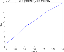
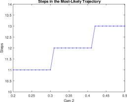
Figure 2: Left sub-plot - Cost of the optimal trajectory vs $w(2)$ in the target histogram $G$. Right sub-plot - number of steps in the optimal trajectory vs $w(2)$ in the target histogram $G$ for target histograms in (8.2).

Simulations with varying target histogram $G$. In the first set of simulations, we consider target histograms

$$G=(0.35,w(2),0.65-w(2)),\text{~{}~{}with~{}}w(2)=0.2,\ldots,0.5.$$ (8.2)

Since histograms with relatively large genotype 2 populations ($w(2)\geq 0.2$) are far from the mean trajectory, populations with such frequencies are rare events. In particular, target histograms in (8.2) correspond to realistic rare events where a genotype with a lower fitness emerges to some significant values before the genotype with the highest fitness dominates the whole population. For instance, the target histogram $G_{1}=[0.35,0.25,0.4]$ corresponds to the event when the frequency of the genotype 2 is approximately 3 times the normal size (compared to mean trajectory) before the whole population is dominated by genotype 3. The target histogram $G_{2}=[0.35,0.35,0.3]$ corresponds to the event when the frequencies of all three genotypes are approximately equal, and the target histogram $G_{3}=[0.35,0.5,0.15]$ corresponds to the population with genotype 2 cells dominating. Most likely trajectories for $G_{1}$, $G_{2}$, and $G_{3}$ are depicted in top-right, bottom-left, and bottom-right parts of Figure 1, respectively.

We also computed other most likely trajectories for target histograms in (8.2) using the step $\Delta w(2)=0.01$. Since the frequency of the genotype 1 is fixed in (8.2), this set of simulations corresponds to a vertical line $w(1)=0.35$. Optimal trajectories for these target histograms are conceptually similar (with a different cost and number of steps) to the most likely trajectories for target histograms $G_{1}$, $G_{2}$, and $G_{3}$. All most likely trajectories for target histograms in (8.2) involve very small shifts in the genetic composition of the population during early stages (i.e. $H\to w_{1}\to w_{2}\to\ldots$). However, these small shifts are rather costly, and early steps in the most likely trajectory comprise a very large percentage of the total cost for the most likely trajectory. These results are presented in detail later in this section and Appendix B.

Figure 2 depicts the cost and the number of steps in most likely trajectories as a function of $w(2)$ in target histograms (8.2). Intuitively, events should become more rare as the frequency of the genotype 2 increases (i.e., target histogram moving away from the mean trajectory). This is confirmed in our simulations. In particular, the left sub-plot of Figure 2 demonstrates that the cost function is a monotonically increasing function of the frequency $w(2)$ in the target histogram. Recall that the probability of each evolutionary trajectory is roughly $P\{{\mathbf{w}}\}\sim e^{-N\Lambda({\mathbf{w}})}$; thus, trajectories with smaller cost $\Lambda({\mathbf{w}})$ are more likely. In addition, the number of steps in the most likely trajectories increases with $w(2)$.

Total trajectory cost as a function of the penultimate point is depicted in Figure 3. The trajectory cost looks like a single-well potential, and the cost grows rapidly outside of a small region around $y^{*}$. Therefore, one can potentially implement a gradient-descent algorithm starting at the point $y^{*},v$ which would significantly accelerate computations compared to a straightforward grid search. Of course, the single-well shape of the cost function cannot be proven in general and needs to be verified for biological models with variables mutation rates, deleterious mutations, and a larger number of genotypes. If the single-well shape of the cost function does not hold in higher dimensions and/or other parameter values, it is possible to implement a probabilistic minimization algorithm similar to the simulated annealing.

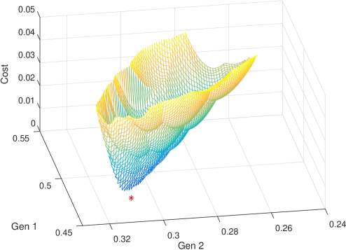
Figure 3: Cost of trajectories connecting the initial histogram $H=[0.99,0.005,0.005]$ and the final histogram $G=[0.35,0.35,0.3]$ as a function of the penultimate point. Red point in the Gen1 - Gen2 plane indicates the $y^{*}\approx[0.475,0.310,0.215]$ computed from conjecture 7.2.

Illustrating Conjectures 7.2, 7.1, 7.3. Next, we illustrate the applicability of Conjectures 7.2, 7.1, 7.3 for a particular target histogram $G=[0.35,0.35,0.3]$. We would like to emphasize that numerical results which are presented here for this particular histogram are generic, and a similar behavior has been confirmed for several other target histograms in (8.2). For the target histogram $G=[0.35,0.35,0.3],$ the solution of the linear system (7.2) in Conjecture 7.2 is $y^{*}\approx[0.47430,0.31043,0.21527]$ while the penultimate point yielding the most likely trajectory for this target histogram is $[0.4752,0.30821,0.21659].$ The difference between these two points is $O(10^{-3})$. This is comparable with the coarse discretization $\epsilon=10^{-3}$ which produced quantitatively similar results. For all target points we investigated, solution of the linear system $y^{*}$ in Conjecture 7.2 was very close to the penultimate point on the most likely trajectory and serves as a natural choice for the center of the set of penultimate points.

Figure 4 depicts upper 5% and 10% quantiles for the values of the function $1/h(y,G)$ discussed in Conjecture 7.1. Table 1 presents values of the constant $c$ for these quantiles for several different target histograms. Figure 4 demonstrates that the upper 5% quantile of the function $1/h(y,G)$ is an adequate choice for the set of penultimate points in the backward search algorithm. The upper 10% quantile set appear to be excessive as a choice of penultimate points in the search algorithm since it covers two evolutionary points on the trajectory. This quantile also covers a considerable region where the frequency of genotype 1 is smaller than 0.35. For the target point with $w(1)=0.35,$ the most likely trajectory would never go through the region with $w(1)<0.35.$ Recovering this genotype back to $0.35$ would be a very costly step due to the fact that this is the genotype with the lowest fitness.

We observe that values of the constant $c$ in Conjecture 7.1 for all target points in Table 1 are extremely small due to the fact that $h(y^{*},G)=O(m)$ and quickly increases away from $y^{*}$. However, Table 1 demonstrates that the constant $c$ is of the same order for different target points and thus roughly independent of the choice of the target histogram $G$. Table 1 also demonstrates that constant $c$ increases slightly when the target histogram moves closer to the boundary. In general, choosing $c\approx 5\times 10^{-6}$ is an adequate choice to define the initial adaptive set of penultimate points in the backward search algorithm for all target histograms $G$.

In practice, implementation of Conjecture 7.1 requires some preliminary exploration of the state space of interior histograms, such as computing quantiles for a few choices of target histograms, computing the corresponding values of $c$, and plotting regions of penultimate points for the backward search algorithm. However, such a preliminary exploration of the state space is rather fast computationally since it does not require computing any trajectories and thus can be quite beneficial computationally for evolutionary problems with a large number of genotypes (e.g., 8 genotypes). We will develop a practical approach using the idea of the adaptive region in subsequent papers for problems with more than 3 genotypes.

Backward search for the most likely trajectory is rather fast computationally for the evolutionary problem with 3 genotypes. Therefore, we also explored the cost of multi-stage trajectories bouncing from the boundary as described in Section 7.3. Typically, there is a small number of incomplete trajectories with an (incomplete) cost which is smaller than the cost of the one-stage optimal trajectory. In particular, we found only 44 incomplete trajectories with an (incomplete) cost which is lower than the cost of one-stage most likely trajectory for the target histogram $G=[0.35,0.35,0.3]$. Out of these 44 trajectories, most of them reach the boundary at a point (histogram) with the frequency of genotype 1 larger than the frequency of genotype 1 in the initial histogram $H$ in (8.1). It is very costly to connect a histogram with $w(1)>0.99$ to the initial histogram $H$ since this corresponds to the event (forward in time) when the frequency of genotype 1 increases for a few steps and then starts decreasing again. This is an extremely unlikely event since genotypes 2 and 3 have higher fitnesses, making them more likely to grow faster than genotype 1.

For several incomplete trajectories terminating at $w_{l}$ in reverse time with $w_{l}(1)<0.99$, the cost of connecting the point $w_{l-1}$ near the boundary with the initial histogram $H$ is very costly. The details of the most likely trajectory connecting $H=[0.99,0.005,0.005]$ and $G=[0.35,0.35,0.3]$ are presented in Table 2. In particular, the cost of the first step $H\to w_{1}$ is the largest in the whole trajectory. This suggests that events in the initial stage (i.e., $H\to w_{1}\to w_{2}\to\ldots$) of any trajectory essentially determine the overall cost of this trajectory.

Initial costs are highly sensitive to the choice of $w_{1}$, $w_{2}$, and so on. This leaves a relatively small set of multi-stage trajectories which can have an overall cost which is lower than the optimal one-stage trajectory. In other words, the numerical investigation of multi-stage trajectories become computationally cheap after a good optimal one-stage candidate has been found. This implies that investigating multi-stage trajectories is a secondary task while the primary problem is finding the optimal one-stage trajectory. In our simulations, we determined that multi-stage trajectories have costs which are significantly higher than the cost of the one-stage most likely trajectory. There is a strong indication that events which correspond to “bouncing away from the boundary” generate costs which are significantly higher than the cost of the initial stages of the one-stage most likely trajectory.

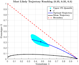
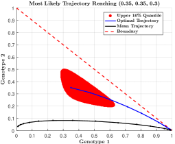
Figure 4: Upper 5% (left sub-plot) and 10% quantiles for the values of $1/h(y,G)$ for the target histogram $G=[0.35,0.35,0.3]$. Note that $y^{*}$ computed as the solution for the linear system (7.2) nearly coincides with the penultimate point for the most likely trajectory. The corresponding values of $c$ in Conjecture 7.1 are $c=7.2\times 10^{-6}$ and $c=4.9\times 10^{-6}$ for the 5% and 10% upper quantile, respectively.

	Quant 5%	Quant 10%
G=[0.35, 0.35, 0.3]	$7.2\times 10^{-6}$	$4.9\times 10^{-6}$
G=[0.35, 0.45, 0.2]	$9.7\times 10^{-6}$	$6.8\times 10^{-6}$
G=[0.2, 0.35, 0.45]	$5.6\times 10^{-6}$	$3.7\times 10^{-6}$
G=[0.2, 0.5, 0.3]	$7.7\times 10^{-6}$	$5.1\times 10^{-6}$
G=[0.2, 0.6, 0.2]	$10.5\times 10^{-6}$	$7.2\times 10^{-6}$

Table 1: Values of $c$ for the upper 5% and 10% quantiles of $1/h(y,G)$ for various target points.

Simulations with varying initial histogram $H$. We consider the target histogram $G=[0.35,0.35,0.3]$ and initial histograms

$$H=(w(1),1-w(1)/2,1-w(1)/2),\text{~{}~{}with~{}}w(1)=0.99,\ldots,0.999.$$ (8.3)

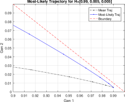
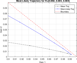
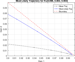
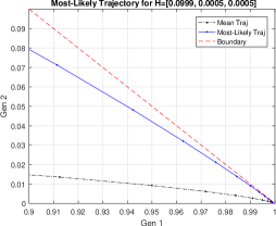
Figure 8: Zoom-in on the initial part of most likely evolutionary trajectories for the population with the target histogram $G=[0.35,0.35,0.3]$ and four different starting histograms. Upper left subplot - starting histogram $H=[0.99,0.005,0.005]$. Upper right subplot - starting histogram $H=[0.992,0.004,0.004]$. Lower left subplot - starting histogram $H=[0.996,0.002,0.002]$. Lower right subplot - starting histogram $H=[0.999,0.0005,0.0005]$.

This corresponds to initial populations with a decreasing frequency of genotypes 2 and 3. Examples of four most likely trajectories and zoom-ins on the initial part of each trajectory are presented in Appendix A. The large-scale aspects of these trajectories look similar. In fact, the difference in penultimate points for these trajectories is $O(10^{-3})$. Since all trajectories are completely determined by their penultimate points, the behaviors of these most likely trajectories near the target histogram $G=[0.35,0.35,0.3]$ are very similar. However, there are subtle differences between these trajectories near the corresponding initial histogram for each trajectory (Figure 8 in Appendix B). We also depict trajectory cost and number of steps in each trajectory vs. $w(1)$ in Figure 5. Numerical values of all points (histograms) in the most likely trajectories for two starting histograms with $w_{0}(1)=0.99$ and $w_{0}(1)=0.999$ together with the cost of each step are presented in Tables 2 and 3 in Appendix B.

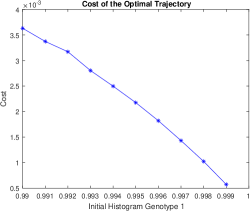
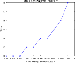
Figure 5: Left sub-plot - Cost of the optimal trajectory vs. $w(1)$ in the initial histogram $H$ in (8.3). Right sub-plot - number of steps in the optimal trajectory vs. $w(1)$ in the initial histogram $H$ in (8.3).

The most likely trajectory reaching $G=[0.35,0.35,0.3]$ starting with $H=[0.99,0.005,0.005]$ is considerably more costly compared with the most likely trajectory starting with $H=[0.999,0.0005,$ $0.0005]$. Therefore, initial populations with a higher frequency of the genotype with the lowest fitness are more likely to exhibit rare events. There are also similarities in both trajectories. In particular, the cost of the few initial steps (e.g., $H\to w_{1}\to w_{2}$) contributes heavily to the overall cost of the trajectory. The fraction of the total cost for each step in the two trajectories for different initial histograms is depicted in Figure 6. In particular, the first step $H\to w_{1}$ corresponds to the event when the frequency of genotype 2 increases much more than the frequency of genotype 3. Obviously, this is a rare event with a low probability. This trend continues in subsequent steps initially so that the frequency genotype 2 reaches large values compared to genotype 3. Such sequences of rare events determine the most likely trajectory describing the global rare event of reaching the target histogram $G$.

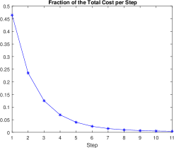
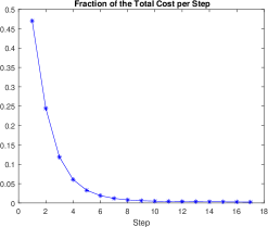
Figure 6: Fraction of the total cost per step for optimal trajectories starting at the initial histogram $H_{0}$ and reaching the final histogram $G=[0.35,0.35,0.3]$. Left sub-plot - trajectory starting at the initial histogram $H=[0.99,0.005,0.005]$ (total cost of this trajectory = 3.630589e-03). Right sub-plot - trajectory starting at the initial histogram $H=[0.999,0.0005,0.0005]$ (total cost of this trajectory = 5.721059e-04).

The costs of each step decay exponentially during the initial stages of the trajectory. We would like to point out that first step in both trajectories is approximately 47% of the total cost, and the first two steps constitute approximately 70% of the total cost. This implies that in most likely trajectories, radical shifts in populations occur early and determine the subsequent evolution of the population.

9 Conclusions

In this paper we presented a novel approach for computing the most likely evolutionary trajectories for rare events in large bacterial populations described by the “locked-box” type models. The approach developed here relies on Large Deviations Theory. In particular, the two most important theoretical results are Theorems 3.16 and 6.1. An explicit formula for the cost function for the transition between two interior histograms is derived in Theorem 3.16. This explicit formula allows for a subsequent construction of the backward search algorithm in Theorem 6.1. These two theorems lay a proper theoretical foundation for a practical implementation of the search algorithm for the most likely evolutionary trajectory connecting two interior histograms.

Numerical implementation of the search algorithm is quite subtle as described in Sections 7.2 and 7.3. In particular, boundary effects need to be potentially taken into account, multi-stage trajectories significantly increase computational time, along with other issues. However, we demonstrated in our numerical examples that all these potential obstacles can be overcome by developing a “smart” search algorithm. Conjectures 7.2 - 7.3 significantly accelerate the search algorithm, and the Large Deviations approach developed here yields an efficient practical tool for investigating various evolutionary scenarios.

We used our approach to investigate a biological system with three genotypes. In particular, our extensive numerical investigation of this system demonstrated the validity of Conjectures 7.2 - 7.3. Moreover, this example elucidates very interesting behavior of the biological system under investigation. For instance, most likely trajectories computed for this example demonstrate that few initial steps correspond to a very large percentage of the total cost. This implies that radical shifts in the frequency of genotypes occur early for rare events and determine the subsequent evolution of the population and emergence of genotypes with a lower fitness.

The numerical approach developed here has been verified on a prototype example with non-reversible advantageous mutations. We also investigated the effect of allowing reversible mutations. We obtained quantitatively similar results (not presented here for the brevity of presentation). In particular, most likely trajectories look quite similar to the examples with non-reversible mutations presented here. We will address the importance of reversible mutations in biological systems with more genotypes in subsequent publications.

The backward search algorithm can be significantly accelerated using Conjectures 7.2 - 7.3. With such accelerated methodology, it stands ready to be applied to more realistic biological systems with up to 8 genotypes. We plan to address the following important questions in subsequent papers - (i) importance of variable mutation rates for different genotypes, (ii) deleterious mutations leading to the decrease in fitness, (iii) mutation matrices representing realistic biological scenarios. In particular, biological examples with 8 genotypes represent bacterial systems with 3 possible mutations. Our numerical approach stands ready to tackle such computationally intensive models. Quantitative investigation of most likely evolutionary trajectories in such realistic examples can potentially shed light on mechanisms for rare events (e.g. emergence or fixation of non-dominant genotypes) in these systems.

Appendix A Most Likely Trajectories for the Target histogram $G=[0.35,0.35,0.3]$ and varying initial histogram $H$

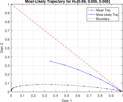
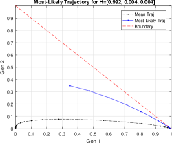
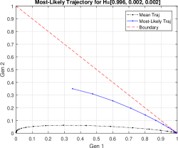
Figure 7: Most likely evolutionary trajectories for the population with the target histogram $G=[0.35,0.35,0.3]$ and four different starting histograms. Upper left subplot - starting histogram $H=[0.99,0.005,0.005]$. Upper right subplot - starting histogram $H=[0.992,0.004,0.004]$. Lower left subplot - starting histogram $H=[0.996,0.002,0.002]$. Lower right subplot - starting histogram $H=[0.999,0.0005,0.0005]$.

Appendix B Most Likely Trajectories for Initial Histograms $[0.99,0.005,0.005]$ and $[0.999,0.0005,0.0005]$

Point #	Gen 1	Gen 2	Gen 3	Cost(${\rm Point}_{i}$, ${\rm Point}_{i+1}$)
1	9.900000e-01	5.000000e-03	5.000000e-03	1.686764e-03
2	9.858695e-01	9.477103e-03	4.653446e-03	8.536793e-04
3	9.780684e-01	1.647496e-02	5.456620e-03	4.539794e-04
4	9.652908e-01	2.709791e-02	7.611302e-03	2.515257e-04
5	9.452312e-01	4.289898e-02	1.186983e-02	1.448337e-04
6	9.144852e-01	6.584684e-02	1.966793e-02	8.682526e-05
7	8.685775e-01	9.805712e-02	3.336541e-02	5.454721e-05
8	8.026050e-01	1.410112e-01	5.638382e-02	3.627721e-05
9	7.130923e-01	1.940756e-01	9.283203e-02	2.581977e-05
10	6.011465e-01	2.527446e-01	1.461089e-01	1.983269e-05
11	4.752100e-01	3.082000e-01	2.165900e-01	1.650544e-05
12	3.500000e-01	3.500000e-01	3.000000e-01

Table 2: Most likely trajectory connecting the starting histogram $H=[0.99,0.005,0.005]$ and the target histogram $G=[0.35,0.35,0.3]$. Length of the trajectory = 12, total cost = 3.630589e-03.

Point #	Gen 1	Gen 2	Gen 3	Cost(${\rm Point}_{i}$, ${\rm Point}_{i+1}$)
1	9.990000e-01	5.000000e-04	5.000000e-04	2.690597e-04
2	9.987909e-01	8.722365e-04	3.368221e-04	1.396945e-04
3	9.982657e-01	1.461233e-03	2.730911e-04	6.773913e-05
4	9.973505e-01	2.365339e-03	2.841971e-04	3.462357e-05
5	9.958865e-01	3.746982e-03	3.664701e-04	1.879674e-05
6	9.935968e-01	5.852370e-03	5.508047e-04	1.090245e-05
7	9.900367e-01	9.051777e-03	9.115416e-04	6.818925e-06
8	9.845097e-01	1.389603e-02	1.594310e-03	4.648979e-06
9	9.759384e-01	2.119084e-02	2.870799e-03	3.472284e-06
10	9.626815e-01	3.208268e-02	5.235793e-03	2.821475e-06
11	9.423048e-01	4.812795e-02	9.567258e-03	2.450309e-06
12	9.113674e-01	7.126889e-02	1.736372e-02	2.224294e-06
13	8.654191e-01	1.035532e-01	3.102764e-02	2.066413e-06
14	7.996234e-01	1.463457e-01	5.403090e-02	1.930059e-06
15	7.105730e-01	1.988617e-01	9.056533e-02	1.787137e-06
16	5.993759e-01	2.564621e-01	1.441620e-01	1.624884e-06
17	4.743500e-01	3.102900e-01	2.153600e-01	1.445064e-06
18	3.500000e-01	3.500000e-01	3.000000e-01

Table 3: Most likely trajectory connecting the starting histogram $H=[0.999,0.0005,0.0005]$ and the target histogram $G=[0.35,0.35,0.3]$. Length of the trajectory = 18, total cost = 5.721059e-04.

References

• [1] R. Azencott. Large deviations theory and applications. In Hennequin P. L., editor, Probbailities at Saint-Flour VIII-1978, pages 1 – 176. Springer Lect. Notes Math. vol 774, 1980.
• [2] R. Azencott, M. I. Freidlin, and S.R.S. Varhadan. Large Deviations at Saint-Flour. Springer, 2012.
• [3] R. Azencott and G.Ruget. Random mixing of differential equations : Large deviations theory. Zeitschrift Wahrschein.Th. und ver. Gebiete, 38:1 – 54, 1977.
• [4] J. E. Barrick and R. E. Lenski. Genome dynamics during experimental evolution. Nature Reviews. Genetics, 14(12):827–839, 2013.
• [5] J. E. Barrick, C. C. Strelioff, R. E. Lenski, and M. R. Kauth. Escherichia coli rpob mutants have increased evolvability in proportion to their fitness defects. Molecular Biology and Evolution, 27(6):1338–1347, 2010.
• [6] N. Champagnat. A microscopic interpretation for adaptive dynamics trait substitution sequence models. Stoch. Proc. Appl., 116(8):1127–1160, 2006.
• [7] N. Champagnat, R. Ferriere, and G. Ben Arous. The canonical equation of adaptive dynamics: A mathematical view. Selection, 2:71–81, 2001.
• [8] N. Champagnat and A. Lambert. Evolution of discrete populations and the canonical diffusion of adaptive dynamics. Ann. Appl. Prob., 17:102–155, 2007.
• [9] Nicolas Champagnat, Régis Ferrière, and Sylvie Méléard. Unifying evolutionary dynamics: From individual stochastic processes to macroscopic models. Theoretical Population Biology, 69(3):297 – 321, 2006. ESS Theory Now.
• [10] V. S. Cooper, D. Schneider, M. Blot, and R. E. Lenski. Mechanisms causing rapid and parallel losses of ribose catabolism in evolving populations of Escherichia coli. Journal of Bacteriology, 183:2834–2841, 2001.
• [11] J. A. Moura de Sousa, P. R. A. Campos, and I. Gordo. An abc method for estimating the rate and distribution of effects of beneficial mutations. Genome Biology and Evolution, 5(5):794–806, 2013.
• [12] Daniel E. Deatherage, Kepner L. Jamie, Albert F. Bennett, Richard E. Lenski, and Jeffrey E. Barrick. Specificity of genome evolution in experimental populations of Escherichia coli] evolved at different temperatures. Proc. Nat. Acad. Sci. USA, 114(10):E1904–E1912, 2017.
• [13] A. Dembo and O. Zeitouni. Large deviations Techniques and applications. Springer-verlag, 1998.
• [14] M. Desai and D. Fisher. Beneficial mutation–selection balance and the effect of linkage on positive selection. Genetics, 176(3):1759–1798, 2007.
• [15] S. F. Levy et al. Quantitative evolutionary dynamics using high-resolution lineage tracking. Nature, 519(7542):181 – 186, 2015.
• [16] Cooper T. F., Rozen D. E., and Lenski R. E. Parallel changes in gene expression after 20,000 generations of evolution in E. coli. Proc. Nat. Acad. Sci. USA, 100:1072–1077, 2003.
• [17] J. W. Fox and R. E. Lenski. From here to eternity - the theory and practice of a really long experiment. PLoS Biology, 13(6):e1002185, 2015.
• [18] I. Gordo, L. Perfeito, and A. Sousa. Fitness effects of mutations in bacteria. Journal of Molecular Microbiology and Biotechnology, 21(1-2):20–35, 2012.
• [19] Matthew Hegreness, Noam Shoresh, Daniel Hartl, and Roy Kishony. An equivalence principle for the incorporation of favorable mutations in asexual populations. Science, 311(5767):1615–1617, 2006.
• [20] C. Illinworth and V. Mustonen. A method to infer positive selection from marker dynamics in asexual population. Bioinformatics, 28(6):831–837, 2012.
• [21] R. Korona, C. H. Nakatsu, L. J. Forney, and R. E. Lenski. Evidence for multiple adaptive peaks from populations of bacteria evolving in a structured habitat. Proc. Nat. Acad. Sci. USA, 91(19):9037–9041, 1994.
• [22] Freidlin M. and Wentzell A. Random perturbations of dynamical systems, volume 260. Springer, 1998.
• [23] F. Peng, S. Widmann, A. Wünsche, K. Duan, K. A. Donovan, R. C. J. Dobson, R. E. Lenski, and T. F. Cooper. Effects of beneficial mutations in pykF gene vary over time and across replicate populations in a long-term experiment with bacteria. Molecular Biology and Evolution, 10(6):msx279, 2017.
• [24] L. D. Plank and J. D. Harvey. Generation time statistics of Escherichia coli B measured by synchronous culture techniques. Journal of General Microbiology, 115:69–77, 1979.
• [25] S. H Rice. Evolutionary Theory. Sinauer Assocites, 2004.
• [26] S. M. Ross. Stochastic Processes. John Wiley $\&$ Sons, New York, 1996.
• [27] D. Simon. Evolutionary Optimization algorithms. John Wiley $\&$ Sons, New York, 2013.
• [28] S. R. S. Varadhan. Large deviations and applications, CBMS-NSF, volume 46. SIAM, 1984.
• [29] F. Vasi, M. Travisano, and R. Lenski. Long-term experimental evolution in Escherichia coli. ii. changes in life-history traits during adaptation to a seasonal environment. The American Naturalist, 144(3):432–456, 1994.
• [30] R. J. Woods, J. E. Barrick, T. F. Cooper, U. Shrestha, M. R. Kauth, and R. E. Lenski. Second-order selection for evolvability in a large Escherichia coli population. Science, 331(6023):1433–1436, 2011.
• [31] W. Zhang, V. Sehgal, D. Dinh, R. R. Azevedo, T. Cooper, and R. Azencott. Estimation of the rate and effect of new beneficial mutations in asexual populations. Theoretical Population Biology, 81(2):168–178, 2012.