Spatially Controllable Image Synthesis with Internal Representation Collaging
Abstract
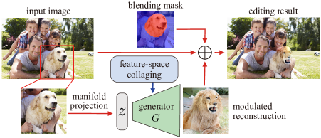
We present a novel CNN-based image editing strategy that allows the user to change the semantic information of an image over an arbitrary region by manipulating the feature-space representation of the image in a trained GAN model. We will present two variants of our strategy: (1) spatial conditional batch normalization (sCBN), a type of conditional batch normalization with user-specifiable spatial weight maps, and (2) feature-blending, a method of directly modifying the intermediate features. Our methods can be used to edit both artificial image and real image, and they both can be used together with any GAN with conditional normalization layers. We will demonstrate the power of our method through experiments on various types of GANs trained on different datasets. Code will be available at https://github.com/pfnet-research/neural-collage.
![[Uncaptioned image]](/html/1811.10153/assets/x1.png)
1 Introduction
Deep generative models like generative adversarial networks (GANs) [10] and variational autoencoders (VAEs) are powerful techniques for the unsupervised learning of latent semantic information that underlies the data. GANs has been particularly successful on the tasks on images: applications include image colorization [14, 16], inpainting [32, 15, 41], domain translation [16, 40, 46, 37, 39], style transfer [12, 42], object transfiguration [45, 24, 13, 22], just to name a few. Generation of photo-realistic images with large diversity has also been made possible by the invention of techniques to stabilize the training process of GANs over massive datasets [26, 11] as well [43, 19, 27, 2, 20].
But the challenge remains to regulate the GANs’ output at the user’s will. In one of the earliest attempts on this problem, conditional GAN [25] established the strategy of concatenating the latent input vector with a vector that represents conditional information. One can change the semantic information of the image by manipulating the conditional vector. InfoGAN [4] further extended the idea by modeling the disentangled latent features with a set of independent conditional vectors and optimizing the model with information theoretic penalty term. More recently, StyleGAN [20] succeeded in automatically isolating the high-level attributes and in realizing a scale-specific control of the image synthesis.
Meanwhile, in creative tasks, for example, it often becomes necessary to transform just small regions of interest in an image. Many methods in practice today use annotation datasets of semantic segmentation. These methods include [16, 39, 31], which can be used to construct a photo-realistic image from a doodle (label map). To author’s best knowledge, however, not much has been done for the unsupervised transformation of images with spatial freedom. Recently, GAN dissection [1] explored the semantic relation between the output and the intermediate features and succeeded in using the inferred relation for photo-realistic transformation. In this paper, we present a strategy of image transformation that is strongly inspired by the findings in [1]. Our strategy is to manipulate the intermediate features of the target image in a trained generator network. We present a pair of novel methods based on this strategy—Spatial conditional batch normalization and Feature blending—that apply affine transformations on the intermediate features of the target image in a trained generator model. Our methods allow the user to edit the semantic information of the image in a copy and paste fashion.
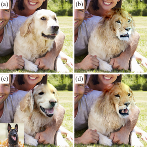
Our Spatial conditional batch normalization is a spatial extension of conditional normalization [5, 33, 12], and it allows the user to blend the semantic information of multiple labels based on the user-specified spatial map of mixing-coefficients (label collaging). With sCBN, we can not only generate an image from a label map but also make local semantic changes to the image like changing the eyes of a husky to eyes of a Pomeranian (Fig. 1a). On the other hand, our Feature blending is a method that directly mixes multiple images in the intermediate feature space, and it enables local blending of more intricate features (feature collaging). With this technique, we can make modifications to the image like changing the posture of an animal without providing the model with the explicit definition of the posture (Fig. 1b).
One significant strength common to both our methods is that they only require a trained GAN that is equipped with AdaIN/CBN structure; there is no need to train an additional model. Our methods can be applied to practically any types of images for which there is a well-trained GAN. Both methods can be used together as well to make an even wider variety of semantic manipulation on images. Also, by combining our methods with manifold projection [44], we can manipulate the local semantic information of a real image (Fig. 2). Our experiments with the most advanced species of GANs [27, 2, 20] shows that our strategy of “standing on the shoulder of giants” is a sound strategy for the task of unsupervised local semantic transformation.
2 Related Work
In this section, we will present the previous literature that are closely related to our study.
Generative adversarial networks (GANs).
GAN is a deep generative framework consisting of a generator function and a discriminator function that play a min-max game in which tries to transform the prior distribution e.g., into a good imposter distribution that mimics the target distribution and tries to distinguish the artificially generated data from the true samples [10]. Thanks to the development of regularization techniques like gradient penalty [11] and spectral normalization [26], deep convolutional GANs [35] are becoming a de facto standard for many image generation tasks. GANs also excel in representation learning, and it is known that one can continuously transform the image in a somewhat semantically meaningful way by interpolating between a pair of points in the latent space [35, 3, 30, 2].
Conditional normalization layers
Classic conditional GAN used to incorporate class-specific information into the output by concatenating a class embedding vector to the latent variable. Becoming more popular in recent years is the strategy of inserting a conditional normalization layer into a network [27, 2, 20, 31]. Conditional batch normalization (CBN) [5, 33] is a mechanism that can learn conditional information in forms of class-specific scaling parameter and shifting parameter. Also belonging to the same family is an adaptive instance normalization (AdaIN) that learns output-conditional scaling parameter and shifting parameter. By manipulating the parameters of the conditional normalization layers, one can manipulate the semantic information of the images in impressively natural fashion.
SPADE [31] is also a method based on conditional normalization that was developed almost simultaneously with our method, and it can learn a function that maps an arbitrary segmentation map to an appropriate parameter map of the normalization layer that can convert the segmentation map to a photo-realistic image. Naturally, the training of the SPADE-model requires a dataset contains annotated segmentation map. However, it can be a nontrivial task to obtain a generator model that is well trained on a dataset of annotated segmentation maps for the specific image-type of interest, let alone the dataset of annotated segmentation map itself. Our method makes a remedy by taking the approach of modifying the conditional normalization layers of a trained GAN. Our spatial conditional batch normalization (sCBN) takes a simple strategy of applying position-dependent affine-transformations to the normalization parameters of a trained network, and it can spatially modify the semantic information of the image without the need of training a new network. Unlike the manipulation done in style transfer [12], we can also edit the conditional information at multiple levels in the network and control the effect of the modification. As we will investigate further in the later section, modification to a layer that is closer to the input tends to transform more global features.
Direct manipulation of intermediate representations
Sometimes, the feature to be transplanted/transformed does not correspond to specific labels/classes. That a specific semantic feature of an image often corresponds to a specific set of neurons in CNN is a fact that has been known from long ago [21]. Numerous approaches have taken advantage of this property of CNN to transfer the styles/attributes of one image to another [9, 38, 23]. Very recently, GAN dissection [1] took a very systematic approach that utilizes the correlation between the intermediate features and semantic segmentation map. By identifying the set of intermediate features that correspond to the semantic feature of interest, GAN dissection succeeded in making modifications to an image like “increasing the number of trees in the park.” One particular advantage of the strategy taken by [1] is that the user does not need to explicitly define the feature that he/she wants to modify in the image when training the generator. Our method is inspired by the findings of [1] and utilizes the conditional information that has already been learned by a trained generator. By blending the intermediate features of multiple images with spatially varying mixture-coefficients, the user can make a wide variety of artificial images without compromising the photo-realism.
3 Two Methods of Collaging the Internal Representations
The central idea common to both our sCBN and Feature blending is to modify the intermediate features of the target image in a trained generator using a user-specifiable masking function. In this section, we will describe the two methods in more formality.
3.1 Spatial Conditional Batch Normalization
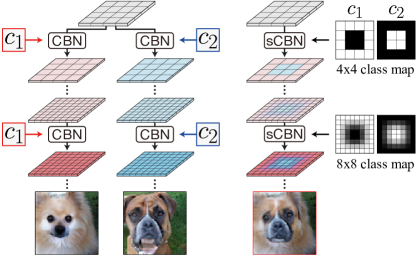
As can be inferred from our naming, spatial conditional batch normalization (sCBN) is closely related to conditional batch normalization (CBN) [7, 5], a variant of Batch Normalization that encodes the class-specific semantic information into the parameters of BN. For locally changing the class label of an image, we will apply spatially varying transformations to the parameters of conditional batch normalization (sCBN) (Fig. 3). Given a batch of images sampled from a single class, the conditional batch normalization [7, 5] normalizes the set of intermediate features produced from the batch by a pair of class-specific scale and bias parameters. Let represent the feature of -th layer at the channel , the height location , and the width location . Given a batch of s generated from a class , the CBN at layer normalizes by:
| (1) |
where are respectively the trainable scale and bias parameters that are specific to the class . The sCBN modifies (1) by replacing with given by
| (2) |
where is a user-selected non-negative tensor map (class-map) of mixture coefficients that integrates to ; that is, for each position . We apply an analogous modification on to produce . If the user wants to modify an artificial image generated by the generator function , the user may replace the CBN of at (a) user-chosen layer(s) with sCBN with (a) user-chosen weight map(s). The region in the feature space that will alter the user-specified region of interest can be inferred with relative ease by observing the downsampling relation in . The user can also control the intensity of the feature of the class at an arbitrary location by choosing the value of (larger the stronger). By choosing to have strong intensities for different classes in different regions, the user can transform multiple disjoint parts of the images into different classes (see figure 1a). As we will show in section 5.3, the choice of the layer(s) in to apply sCBN have interesting effects on the intensity of the transformation. The figure 3 shows the schematic overview of the mechanism of sCBN. By using manifold projection, sCBN can be applied to real images as well. We will elaborate more on the application of our method to real images in section 4.
3.2 Spatial Feature Blending
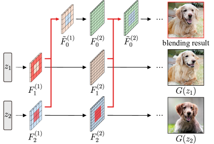
Our spatial feature blending is a method that can extract the features of a particular part of one image and blend it into another. Suppose that images are generated from latent variables by a trained generator , and that are the feature map of the image that can be obtained by applying layers of to . We can then blend the features of into by recursively replacing with
| (3) |
where is the Hadamard product, is the user-specified non-negative tensor (feature blending weights) with the same dimension as such that is the tensor whose entries are all , and is an optional shift operator that uniformly translate the feature map to a specified direction, which can be used to move a specific local feature to an arbitrary position.
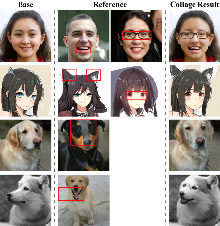
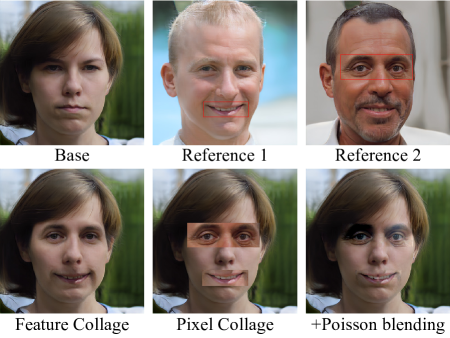
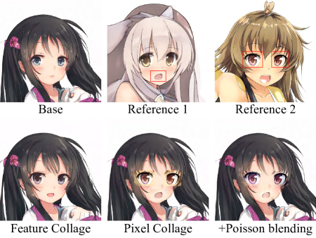
As a map that is akin to the class map in sCBN, the user may choose in a similar way as in the previous section to spatially control the effect of the blending. Spatial feature blending can also be applied to real images by using the method of manifold projection. The figure 4 is an overview of the feature-blending process in which the goal is to transplant a feature (front facing open mouth) of an image to the target image (a dog with a closed mouth). All the user has to do in this scenario is to provide a mixing map that has high intensity on the region that corresponds to the region of the mouth. As we will show in the experiment section, our method is quite robust to the alignment, and the region of mouth in and needs to be only roughly aligned.
4 Application to Real Images
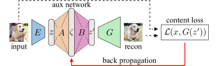
To edit the semantic information of a real image, we can use the method of manifold projection [44] that looks for the latent variable such that . After obtaining the inverse of , we can apply the same set of procedures we described above to either modify the label information of parts of or blend the features of other images into or do both. The figure 5 is the flow of real-image editing.
We will describe this process in more formality. Let be the pair of a trained generator and a discriminator. Given an image of interest (often a clip from a larger image), the first goal of the manifold projection step is to train the encoder such that is small for some dissimilarity measure . The choice of in our method is the cosine distance in the final feature space of the discriminator . That is, if is the normalized feature of the image in the final layer of ,
| (4) |
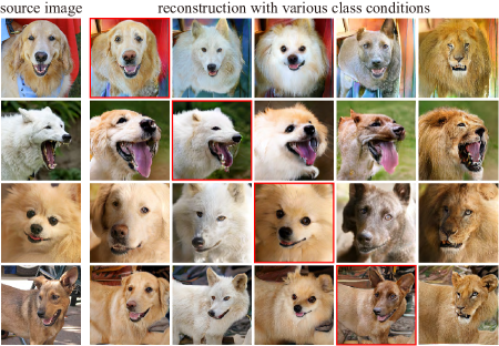
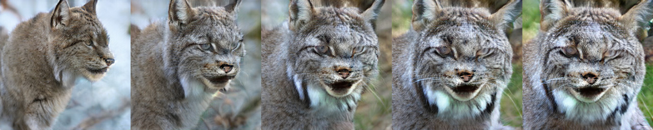
After training the encoder, one can produce the reconstruction of by applying to . In the reconstructed image, however, semantically independent objects can be dis-aligned. We, therefore, calibrate by additionally backpropagating the loss . After some rounds of calibration, we can feed the obtained to the modified to create a transformed reconstruction. Please see the supplementary material for the details of the manifold projection algorithm. The figure 6 shows examples of reconstruction with various class conditions.
As a final touch to the transformed image, we apply a post-processing step of Poisson blending [34]. Because most trained GAN models do not have the ability to disentangle objects from the background, naively pasting the generated clip to the target image can produce artifacts in the region surrounding the object of interest. We can clean up these artifacts with Poisson blending to the region of interest.
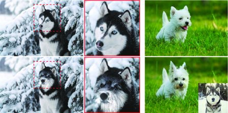
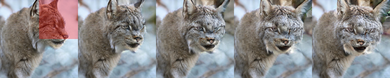
Fig. 7 are examples of the application of our methods to real images. The image in the left panel is an application of sCBN to a real image, and the image in the right panel is an application of feature blending to a real image.
5 Experiments
In this section, we present the results of our experiments together with the experimental settings. For further details, please see the supplementary material.
5.1 Experimental Settings
We applied our methods to ResNet-based generators that were trained as parts of conditional GANs: SNGAN [26, 27], BigGAN [2], and StyleGAN [20]. These GANs are all equipped with conditional normalization layers. In the experiments, we treated the AdaIN layer in the StyleGAN in the same manner as the conditional batch normalization layer. Both SNGAN and BigGAN used in our study first map the latent vector into feature maps of dimension , and doubles the resolution at every ResBlock to produce an RGB image of the user-specified dimensions in the final layer. We produced both (for Flowers dataset) and (for Dogs+Cats dataset) images with SNGAN, and produced images with BigGAN. The StyleGAN used in this study produces the image of 1024 1024 resolution by recursively applying convolution layers and AdaIN layers to the latent vector.
5.2 Results
| Dataset | Model |
|---|---|
| ∗Dogs+Cats (143 classes)111subset of ImageNet [36] | SNGAN [26, 27] |
| Flowers (102 classes) [29] | |
| ∗ImageNet (1000 classes) [36] | BigGAN [2] |
| ∗FFHQ222https://github.com/NVlabs/ffhq-dataset | StyleGAN [20] |
| Danbooru (anime face)333https://www.gwern.net/Danbooru2018 |
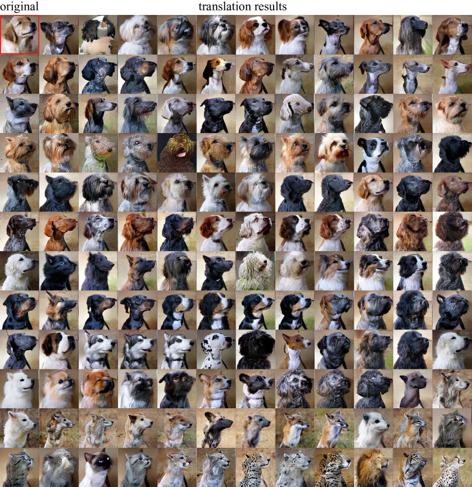
We demonstrate the utility of our algorithm with several DCGANs trained on different image datasets (see figure 1). In order to verify the representation power of our manifold projection method and the DCGANs used in our study, we conducted a set of ablation experiments for non-spatial transformation as well. We confirmed that the generators used in our study are powerful enough to capture the class-invariant intermediate features (see figure 6 and the supplementary material).
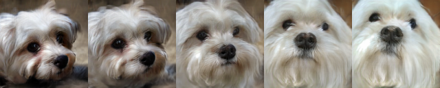
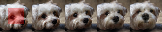
The images in figure 8 are examples of our label collaging with sCBN. We see that our transformation is modulating both global information (e.g. face/shape) and local information (e.g. color/texture) without breaking the semantic consistency. Also, note that areas outside the specified region are also affected when global features like “face of a dog” are altered. Interestingly, our algorithm is automatically choosing the region to be influenced by the modification of global feature so that there will not be an unnatural discontinuity in the transformed image. Because the user-specified region of interest is defined in the pixel space, this observation suggests that the algorithm is modulating the global features in the layers close to the input. Because the user is allowed to assign continuous values to the label map, the intensity of collaging can be continuously controlled as well (see figure 9).
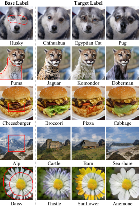
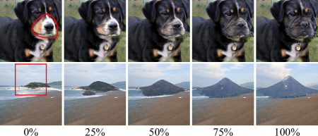
Figure 10 shows the examples of our feature blending. We are succeeding in making semantic modifications like “changing the posture of a dog”, “changing the style of a part of an anime character” without destroying the quality of the original image. We also can see that the performance is robust against the alignment of the region to be transformed. We emphasize that we are succeeding in creating these transformations without using any information about the attributes to be altered. Also note the difference in the results between our method and the simple interpolation in the latent space (figure 11). As we can see in the result, our method can maintain the semantic context outside the specified region. We see that we are succeeding in controlling the region to be modified with the user-specifiable map of mixing coefficients.
5.3 The Effect of Collaging at Each Layer
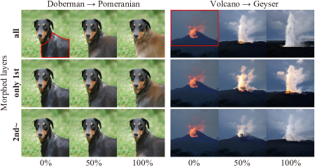
We conducted a set of ablation studies to investigate the influence of the modification at each layer. The images in the figure 12 are results obtained by applying sCBN to (1) all layers, (2) the layer closest to the input (first layer), and (3) all the layers except the first layer. As we mentioned in the previous section, the layers closer to tend to influence more global features, and the layers closer to tend to influence more local features. As we can see in the figure, the features affected by the manipulation of the layers close to (body shape of dog, ridge line of mountain) are somewhat semantically independent from the features affected by the layers close to (fur texture, local features of “lava”).
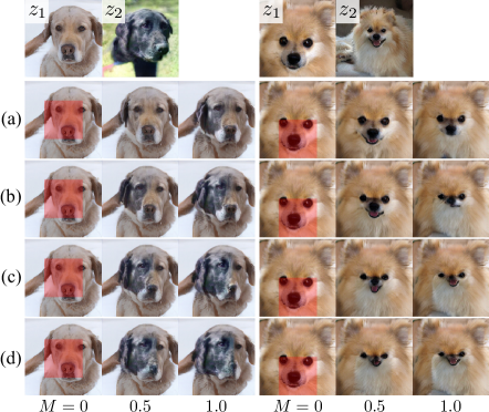
Figure 13 shows the result of applying the feature blending to different layers () with different blending weights. When the blending is applied exclusively to the layer (closest to the input), the global features like “body shape of a dog” is affected, and local features like “fur textures” are preserved.. We observe the opposite effect when the blending is applied to the layers closer to . Also, when the reference image is significantly different from the target image in terms of its topology, the exclusive modification to the layers close to tends to produce artifacts.
These results suggest that, if necessary, we may customize our method to more finely control the locality and the intensity of the transformation by applying our methods with carefully chosen mixture-of-coefficient maps to each layer.
5.4 Real Image Transformation
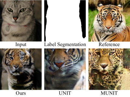
In order to provide some quantitative measurement for the quality of our real image transformation, we evaluated the fidelity of the transformed images with classification accuracy and human perceptual test. We applied our sCBN to the real images in ImageNet and conducted the translation of (1) cat big cat, (2) cat dog, and (3) dog dog, and evaluated the classification accuracy of the transformed images by an inception-v3 classifier trained on ImageNet for the classification of 1000 classes. For each pair of image-domains, we selected four classes from both source and target domains, and conducted 1000 tasks of translating an image of a randomly selected source class to a randomly selected target class (e.g., one feline species to one canine species). We used UNIT [24] and MNUIT [13] as baselines. Because MUNIT is not designed for class-to-class translation, we conducted MUNIT using the set of images in the target class as the reference images. Table 2 summarizes the result. For each set of translation task, our method achieved better top-5 error rate than the other methods. This result confirms the efficacy of our method of real image transformation.
| Method | cat big cat | cat dog | dog dog |
|---|---|---|---|
| Ours | 7.8% | 21.1% | 20.8% |
| UNIT | 14.8% | N/A | 36.2% |
| MUNIT | 26.0% | 55.4% | N/A |
We used Amazon Mechanical Turk (AMT) for a human-perceptual test. We asked each AMT worker to decide if the transformed images produced by our method are more photo-realistic than the images produced by MUNIT/UNIT. For each comparison, we used 200 AMT workers for the evaluation and asked each worker to make votes for 10 pair of images. Table 3 is the summary of the result. We see that our method outperforms both MUNIT and UNIT for the translations in all pairs of domains. Our method is also capable of many-to-many translation over a set of 100 or more classes (see the supplementary material).
| vs. | cat big cat | cat dog | dog dog |
|---|---|---|---|
| UNIT | % | N/A | % |
| MUNIT | 75.4% | % | N/A |
6 Conclusions
By construction, our method is limited by the ability of the used generator. Our method simply cannot make expressions beyond the representation power of the used generator. This limitation is particularly true when we apply our method together with manifold projection to transform a real image. For example, our method is likely to perform poorly in the transformation of the image of a specific individual unless the used generator is capable of accurately reconstructing the face of the target individual. The process of manifold projection projects the target image to the restricted space of images that are reconstructable by the used generator, and some information is bound to be lost in the process.
We shall also make some remark about the weakness of our feature blending. As we described throughout the text, the main strength of our feature blending is that it does not require the user to provide the explicit definition of the feature to be blended. It is very natural that this advantage comes at the cost of blending the feature that is not intended to be blended. Because we ask the user to specify just the source region from which to extract the feature, all features that are contained in the user-specified region become subject to the blending process. We may be able to further fine-tune the image synthesis by using the method in [1] to identify the specific unit in the internal feature space that corresponds to the target feature to be transferred.
Also, conditional normalization layers are capable of handling not only class conditions but other types of information like verbal statements as well. One might be able to conduct an even wider variety of spatial transformation by making use of them. Applications of our method to non-image dataset is also an interesting direction for future work.
Acknowledgements
We would like to acknowledge Jason Naradowsky, Masaki Saito, Jin Yanghua, and Atsuhiro Noguchi for helpful insights and suggestions.
References
- [1] D. Bau, J.-Y. Zhu, H. Strobelt, B. Zhou, J. B. Tenenbaum, W. T. Freeman, and A. Torralba. GAN dissection: Visualizing and understanding generative adversarial networks. In Proceedings of the International Conference on Learning Representations (ICLR), 2019.
- [2] A. Brock, J. Donahue, and K. Simonyan. Large scale gan training for high fidelity natural image synthesis. arXiv:1809.11096, 2018.
- [3] A. Brock, T. Lim, J. M. Ritchie, and N. Weston. Neural photo editing with introspective adversarial networks. In Proceedings of the International Conference on Learning Representations (ICLR), 2017.
- [4] X. Chen, Y. Duan, R. Houthooft, J. Schulman, I. Sutskever, and P. Abbeel. Infogan: Interpretable representation learning by information maximizing generative adversarial nets. In Advances in Neural Information Processing Systems (NIPS), pages 2172–2180, 2016.
- [5] H. De Vries, F. Strub, J. Mary, H. Larochelle, O. Pietquin, and A. C. Courville. Modulating early visual processing by language. In Advances in Neural Information Processing Systems (NIPS), pages 6594–6604, 2017.
- [6] A. Dosovitskiy and T. Brox. Generating images with perceptual similarity metrics based on deep networks. In Advances in Neural Information Processing Systems, pages 658–666, 2016.
- [7] V. Dumoulin, J. Shlens, and M. Kudlur. A learned representation for artistic style. In Proceedings of the International Conference on Learning Representations (ICLR), 2017.
- [8] C. Finn, P. Abbeel, and S. Levine. Model-agnostic meta-learning for fast adaptation of deep networks. In Proceedings of the International Conference on Machine Learning (ICML), pages 1126–1135, 2017.
- [9] L. A. Gatys, A. S. Ecker, and M. Bethge. A neural algorithm of artistic style. arXiv preprint arXiv:1508.06576, 2015.
- [10] I. Goodfellow, J. Pouget-Abadie, M. Mirza, B. Xu, D. Warde-Farley, S. Ozair, A. Courville, and Y. Bengio. Generative adversarial nets. In Advances in neural information processing systems (NIPS), pages 2672–2680, 2014.
- [11] I. Gulrajani, F. Ahmed, M. Arjovsky, V. Dumoulin, and A. C. Courville. Improved training of wasserstein gans. In Advances in Neural Information Processing Systems (NIPS), pages 5767–5777, 2017.
- [12] X. Huang and S. J. Belongie. Arbitrary style transfer in real-time with adaptive instance normalization. In Proceedings of the International Conference on Computer Vision (ICCV), pages 1510–1519, 2017.
- [13] X. Huang, M.-Y. Liu, S. Belongie, and J. Kautz. Multimodal unsupervised image-to-image translation. In Proceedings of the European Conference on Computer Vision (ECCV), pages 179–196, 2018.
- [14] S. Iizuka, E. Simo-Serra, and H. Ishikawa. Let there be color!: joint end-to-end learning of global and local image priors for automatic image colorization with simultaneous classification. ACM Transactions on Graphics (TOG), 35(4):110:1–110:11, 2016.
- [15] S. Iizuka, E. Simo-Serra, and H. Ishikawa. Globally and locally consistent image completion. ACM Transactions on Graphics (TOG), 36(4):107:1–107:14, 2017.
- [16] P. Isola, J. Zhu, T. Zhou, and A. A. Efros. Image-to-image translation with conditional adversarial networks. In Proceedings of the IEEE Conference on Computer Vision and Pattern Recognition (CVPR), pages 5967–5976, 2017.
- [17] J. Johnson, A. Alahi, and L. Fei-Fei. Perceptual losses for real-time style transfer and super-resolution. In Proceedings of the European Conference on Computer Vision (ECCV), pages 694–711, 2016.
- [18] T. Kaneko, K. Hiramatsu, and K. Kashino. Generative attribute controller with conditional filtered generative adversarial networks. In Proceedings of the IEEE Conference on Computer Vision and Pattern Recognition (CVPR), pages 7006–7015, 2017.
- [19] T. Karras, T. Aila, S. Laine, and J. Lehtinen. Progressive growing of GANs for improved quality, stability, and variation. In Proceedings of the International Conference on Learning Representations (ICLR), 2018.
- [20] T. Karras, S. Laine, and T. Aila. A style-based generator architecture for generative adversarial networks. In Proceedings of the IEEE Conference on Computer Vision and Pattern Recognition (CVPR), 2019.
- [21] Q. V. Le, M. Ranzato, R. Monga, M. Devin, K. Chen, G. S. Corrado, J. Dean, and A. Y. Ng. Building high-level features using large scale unsupervised learning. In Proceedings of the International Conference on Machine Learning (ICML), pages 507–514, 2012.
- [22] X. Liang, H. Zhang, L. Lin, and E. Xing. Generative semantic manipulation with mask-contrasting GAN. In Proceedings of the European Conference on Computer Vision (ECCV), pages 558–573, 2018.
- [23] J. Liao, Y. Yao, L. Yuan, G. Hua, and S. B. Kang. Visual attribute transfer through deep image analogy. ACM Trans. Graph., 36(4):120:1–120:15, July 2017.
- [24] M.-Y. Liu, T. Breuel, and J. Kautz. Unsupervised image-to-image translation networks. In Advances in Neural Information Processing Systems (NIPS), pages 700–708, 2017.
- [25] M. Mirza and S. Osindero. Conditional generative adversarial nets. arXiv preprint arXiv:1411.1784, 2014.
- [26] T. Miyato, T. Kataoka, M. Koyama, and Y. Yoshida. Spectral normalization for generative adversarial networks. In Proceedings of the International Conference on Learning Representations (ICLR), 2018.
- [27] T. Miyato and M. Koyama. cGANs with projection discriminator. In Proceedings of the International Conference on Learning Representations (ICLR), 2018.
- [28] T. Munkhdalai, X. Yuan, S. Mehri, and A. Trischler. Rapid adaptation with conditionally shifted neurons. In Proceedings of the International Conference on Machine Learning (ICML), pages 3661–3670, 2018.
- [29] M.-E. Nilsback and A. Zisserman. Automated flower classification over a large number of classes. In Proceedings of the Indian Conference on Computer Vision, Graphics and Image Processing, 2008.
- [30] A. Odena, C. Olah, and J. Shlens. Conditional image synthesis with auxiliary classifier GANs. In Proceedings of the International Conference on Machine Learning (ICML), volume 70 of Proceedings of Machine Learning Research, pages 2642–2651, International Convention Centre, Sydney, Australia, 2017. PMLR.
- [31] T. Park, M.-Y. Liu, T.-C. Wang, and J.-Y. Zhu. Semantic image synthesis with spatially-adaptive normalization. In Proceedings of the IEEE Conference on Computer Vision and Pattern Recognition (CVPR), 2019.
- [32] D. Pathak, P. Krahenbuhl, J. Donahue, T. Darrell, and A. A. Efros. Context encoders: Feature learning by inpainting. In Proceedings of the IEEE Conference on Computer Vision and Pattern Recognition (CVPR), pages 2536–2544, 2016.
- [33] E. Perez, F. Strub, H. De Vries, V. Dumoulin, and A. Courville. Film: Visual reasoning with a general conditioning layer. In Proceedings of the AAAI Conference on Artificial Intelligence (AAAI), pages 3942–3951, 2018.
- [34] P. Pérez, M. Gangnet, and A. Blake. Poisson image editing. ACM Transactions on graphics (TOG), 22(3):313–318, 2003.
- [35] A. Radford, L. Metz, and S. Chintala. Unsupervised representation learning with deep convolutional generative adversarial networks. In Proceedings of the International Conference on Learning Representations (ICLR), 2016.
- [36] O. Russakovsky, J. Deng, H. Su, J. Krause, S. Satheesh, S. Ma, Z. Huang, A. Karpathy, A. Khosla, M. Bernstein, A. C. Berg, and L. Fei-Fei. Imagenet large scale visual recognition challenge. International Journal of Computer Vision, 115(3):211–252, 2015.
- [37] P. Sangkloy, J. Lu, C. Fang, F. Yu, and J. Hays. Scribbler: Controlling deep image synthesis with sketch and color. In Proceedings of the IEEE Conference on Computer Vision and Pattern Recognition (CVPR), volume 2, pages 5400–5409, 2017.
- [38] P. Upchurch, J. Gardner, G. Pleiss, R. Pless, N. Snavely, K. Bala, and K. Weinberger. Deep feature interpolation for image content changes. In Proceedings of the IEEE Conference on Computer Vision and Pattern Recognition (CVPR), pages 7064–7073, 2017.
- [39] T.-C. Wang, M.-Y. Liu, J.-Y. Zhu, A. Tao, J. Kautz, and B. Catanzaro. High-resolution image synthesis and semantic manipulation with conditional GANs. In Proceedings of the IEEE Conference on Computer Vision and Pattern Recognition (CVPR), pages 8798–8807, 2018.
- [40] Z. Yi, H. R. Zhang, P. Tan, and M. Gong. Dualgan: Unsupervised dual learning for image-to-image translation. In Proceedings of the International Conference on Computer Vision (ICCV), pages 2868–2876, 2017.
- [41] J. Yu, Z. Lin, J. Yang, X. Shen, X. Lu, and T. S. Huang. Generative image inpainting with contextual attention. In Proceedings of the IEEE Conference on Computer Vision and Pattern Recognition (CVPR), pages 5505–5514, 2018.
- [42] H. Zhang and K. Dana. Multi-style generative network for real-time transfer. arXiv preprint arXiv:1703.06953, 2017.
- [43] H. Zhang, I. Goodfellow, D. Metaxas, and A. Odena. Self-attention generative adversarial networks. In Proceedings of the IEEE Conference on Computer Vision and Pattern Recognition (CVPR), 2018.
- [44] J.-Y. Zhu, P. Krähenbühl, E. Shechtman, and A. A. Efros. Generative visual manipulation on the natural image manifold. In Proceedings of the European Conference on Computer Vision (ECCV), pages 597–613, 2016.
- [45] J.-Y. Zhu, T. Park, P. Isola, and A. A. Efros. Unpaired image-to-image translation using cycle-consistent adversarial networks. In Proceedings of the International Conference on Computer Vision (ICCV), pages 2242–2251, 2017.
- [46] J.-Y. Zhu, R. Zhang, D. Pathak, T. Darrell, A. A. Efros, O. Wang, and E. Shechtman. Toward multimodal image-to-image translation. In Advances in Neural Information Processing Systems (NIPS), pages 465–476, 2017.
Appendix A Implementation in Various GANs
Our label collaging method can be applied to any GAN equipped with conditional normalization layers (e.g., CBN, AdaIN) by replacing the layers with their spatial variants. Our feature collaging method can be applied to any GAN as well by specifying the intermediate feature maps to be manipulated. For the ResNet-based architectures like SNGAN and BigGAN, we chose to manipulate the output feature map and the first 44 feature map of each ResBlock. For StyleGAN, we chose to manipulate the output of each Synthesis Block. Each Synthesis Block consists of two AdaIn layers, one upsampling operator and one convolution layer.
Appendix B Fast Manifold Projection
In order to enable the semantic modification of real images in real time, we explored a way to speed up the manifold projection step. Our implementation was able to speed up the process by more than 30%.
B.1 Latent Space Expansion with Auxiliary Network
Image features are generally entangled in the latent space of a generative model, and the optimization on the complex landscape of loss can be time-consuming. To speed up the process, we construct an auxiliary network that embeds in higher dimensional space. The auxiliary network consists of an embedding map that converts into high dimensional , and a projection map that converts back to (figure 14). That is, instead of calibrating the latent variable by backpropagating through , we will calibrate by backpropagating through and . The goal of training this auxiliary network is to find the map that allows us to represent the landscape of in a form that is more suitable for optimization, together with the map that can embed in a way that is well-suited for the learning on the landscape. Let be the variable in the high dimensional latent space after rounds of calibration. The update rule of we use here is
| (5) |
where is the length parameter at the -th round. We train the networks and using the following loss function:
| (6) |
where constants determine the importance of the -th round of the calibration. For the first term, and are updated through the backpropagation from . The second term makes sure that can be reconstructed from . This process can be seen as a variant of meta-learning [8, 28].
For the auxiliary maps and , we used a -layer MLP with hidden units of size equipped with a trainable PReLU activation function at respective layers, and treated the 10000-dimensional layer as the extended latent variable . For the evaluation of , we used , , and .
B.2 Training Procedure
We trained the three components of the model (, , ) separately, in order. We first trained a pair of generator and discriminator by following the procedure of conditional GANs described in [26, 27]. We then trained the encoder network (figure 15) for the trained generator using the objective function defined based on the trained discriminator (see the main section in the article about the manifold projection). Finally, fixing the encoder and the generator we trained, we trained the auxiliary networks to enhance the manifold-embedding optimization.

For the training of the auxiliary network, we used AdaGrad with adaptive learning rate for the gradient descent to calculate . We used AdaGrad for this procedure because other methods (e.g., Adam) causes numerical instability in double backpropagation for network parameter update. We trained each model over iterations. For the training of auxiliary networks, we applied the gradient clipping with the threshold of and the weight decay at the rate of . We trained the networks on a GeForce GTX TITAN X for about a week for each component.
B.3 Speed-up by Latent Space Expansion
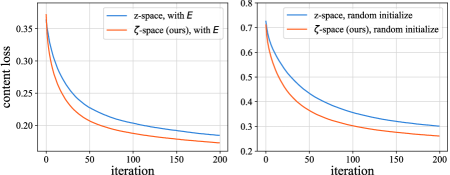
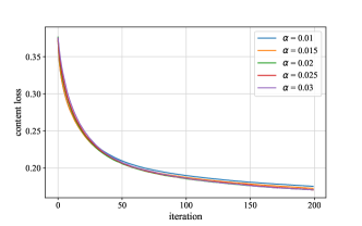
We conducted an experiment to verify that our auxiliary network can indeed speed up the optimization process. We used the DCGANs trained on the dog+cat dataset and evaluated the average loss for 1000 images randomly selected from ImageNet. The optimization was done with Adam, implemented with the best learning rate in the search-grid that achieved the fastest loss decrease. Figure 16 compares the transition of the loss function learned on -latent space against the loss transition produced on -latent space. To decrease the loss by the same amount, the learning of required only less than the number of iterations required by the learning of . Calculation overhead due to the latent space expansion was negligible (%). Indeed, the learning process depends on the initial value of the latent variable or . When compared to random initialization, the optimization process on both space and space proceeded faster when we set the initial value at and . This result is indicative of the importance of training . We also studied the robustness of our manifold projection algorithm against the choice of the hyper-parameter. We performed optimization with various learning rates of Adam for updating . Our study suggests that our algorithm is quite robust with respect to the learning rate.
Appendix C Internal Representation Collage vs. Pixel-space Collage
Our methods modify the target image by manipulating its intermediate representation in the generator’s feature space. The most prominent advantage of this strategy is that it allows the generator to automatically adjust the spatially varying intensity of the modification to make the final output natural. In this section, we compare the results of our method against the most basic collaging method of modifying the image in the pixel space pixel collage. The images in the Figure 18 are the results of label collaging for an image obtained from the same latent variable. As we see in Figure 18, the result of pixel collage is deformed/blurry even after the post-processing of Poisson blending, and the boundary of modified regions is unnatural. On the other hand, our method is automatically adjusting the intensity to naturally match the modified region and the neighboring region (e.g., mouth shape, shoreline).
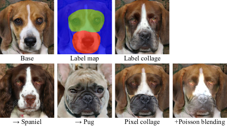
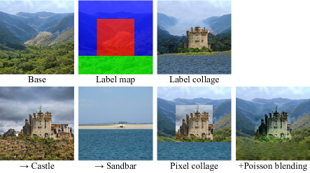
Figure 19 compares our feature collaging against the naive pixel space collaging. Notice that our method is not creating any artifacts around the modified regions. On the other hand, the image created by pixel space collaging is strongly deformed/blurry around the region of modification, even after the application of Poisson blending.
Appendix D Real Image Transformation Study
For evaluating the fidelity of real image transformation, we conducted a set of automatic spatial class translations. For each one the selected images, we (1) used a pre-trained model to extract the region of the object to be transformed (dog/cat), (2) conducted the manifold projection to obtain the , (3) passed to the generator with the class map corresponding to the segmented region, and (4) conducted post-processing over the segmented region. For the semantic segmentation, we used a TensorFlow implementation of DeepLab v3 Xception model trained on MS COCO dataset111https://github.com/tensorflow/models/tree/master/research/deeplab. See Figure 20 for the transformation examples.
Appendix E Global Translation of Real Image
In order to verify the sheer ability of our translation method, we conducted a translation task for the entire image as well (as opposed to the translation for a user-specified subregion). For each of the selected images from the ImageNet, we calculated a latent encoding variable , and applied a set of spatial uniform class-condition to the layers of the decoder. Figure 21 contains the translation of a real image (designated as original) to all 143 object classes that were used for the training of the dog+cat model. We can see that the semantic information of the original image is naturally preserved in most of the translations.