Heating and Cooling of Quantum Gas by Eigenstate Joule Expansion
Abstract
We investigate the Joule expansion of an interacting quantum gas in an energy eigenstate. The Joule expansion occurs when two subsystems of different particle density are allowed to exchange particles. We demonstrate numerically that the subsystems in their energy eigenstates evolves unitarily into the global equilibrium state in accordance with the eigenstate thermalization hypothesis. We find that the quantum gas changes its temperature after the Joule expansion with a characteristic inversion temperature . The gas cools down (heats up) when the initial temperature is higher (lower) than , implying that is a stable fixed point, which is contrasted to the behavior of classical gases. Our work exemplifies that transport phenomena can be studied at the level of energy eigenstates.
pacs:
05.30.-d,05.70.Ln,03.65.AaIntroduction — Statistical mechanics postulates that an isolated quantum system in thermal equilibrium is represented by the completely mixed state in the microcanonical energy shell. It has been a puzzling question whether statistical mechanics is compatible with unitary dynamics of quantum mechanics which does not allow a transition of a pure state to a mixed state. Recent studies have revealed that this puzzle can be settled in view of quantum ergodicity D’Alessio et al. (2016). A quantum mechanical system in a pure state can be thermal by itself. That is, the system, if quantum chaotic, plays a role of an equilibrium heat bath for its subsystem as if it were in the equilibrium mixed state. In fact, the eigenstate thermalization hypothesis (ETH) asserts that all the energy eigenstates are thermal for a broad class of non-integrable quantum systems Srednicki (1994); Deutsch (1991); Kim et al. (2014); Yoshizawa et al. (2018); Rigol (2009); von Neumann (2010); Beugeling et al. (2014).
The ETH has been tested numerically in various discrete lattice systems. Those studies confirm that the expectation value of local observables in the energy eigenstate is consistent with the statistical mechanics prediction Jensen and Shankar (1985); Rigol et al. (2008); Kim et al. (2014); Yoshizawa et al. (2018). They also confirm that quantum systems thermalize after a quench, a sudden change in the Hamiltonian, following the ETH prediction Rigol (2009). The thermalization of isolated quantum systems has also been studied experimentally using ultracold atoms Kinoshita et al. (2006); Tang et al. (2018); Trotzky et al. (2012); Langen et al. (2015); Kaufman et al. (2016); Kim et al. (2018) and superconducting qubits Neill et al. (2016). The ETH is now recognized as a paradigm of statistical mechanics for pure quantum systems with a few notable exceptions such as the integrable systems Biroli et al. (2010), the many-body localization systems Imbrie (2016), systems with many-body quantum scars Turner et al. (2018); Shiraishi and Mori (2017); *Mondaini:2018jo; *Shiraishi:2018gc.
Besides a single isolated system, it is also interesting to ask how two quantum systems thermalize in the presence of a thermal contact. Ponomarev et al. demonstrated numerically the thermalization of two systems which exchange the energy Ponomarev et al. (2011). A thermal contact may also allow the exchange of a globally conserved entity such as the particle number. Yet, the quantum thermalization under such a contact has been studied rarely.
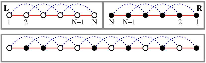
The Joule expansion is a representative irreversible process taking place under the general contact Reif (1965); Blundell and Blundell (2006). Suppose that a gas is confined in a compartment of an isolated container (see Fig. 1). When the dividing wall is removed or a contact opens, the gas expands irreversibly and reaches the homogeneous equilibrium state. The Joule expansion in the classical regime is well understood. For instance, the Van der Waals gases cool down upon expansion because gas particles loose the kinetic energy gaining the attractive interaction potential energy Blundell and Blundell (2006). A mean field study with the Lennard-Jones potential showed that the classical gases can heat up if the initial temperature is high above a threshold , called the inversion temperature Goussard and Roulet (1993). The short range repulsion between particles is responsible for the inversion temperature.
In this Letter, we investigate the thermalization of two quantum systems coupled by an interaction Hamiltonian which allows the exchange of particles as well as the energy. Both subsystems are in their respective energy eigenstates, and evolve unitarily into a steady state after the interaction turns on. With this setup, we can study the Joule expansion of an interacting quantum gas in an energy eigenstate *[TheJouleexpansionofnoninteractingquantumgaswasstudiedin][.]Camalet:2008fg. We demonstrate that there exists an inversion temperature : The quantum gas cools down (heats up) when the initial temperature is above (below) , which makes the inversion temperature stable. This is in sharp contrast to the behavior of the classical gases which heats up when the initial temperature is above an inversion temperature, which suggests that the inversion temperature results from a many-body correlation effect in the quantum case. The Joule expansion can be realized experimentally using ultracold gases Schneider et al. (2012). We anticipate that our result will be relevant for controlling temperature in such experimental setups.
Model — For concreteness, we present our work in the context of a spin chain system. We consider the two identical spin-1/2 XXZ chains of length , referred to as L and R, with nearest and next nearest neighbor interactions (see Fig. 1). The Hamiltonian of each chain = L, R reads
| (1) |
with the two-body interaction Hamiltonian
| (2) |
Here, denotes the Pauli matrix for a spin at site in the chain . The model includes a few parameters: sets the scale of energy, is the anisotropy parameter, and represents the relative strength of the next nearest neighbor interactions. With nonzero , the system is known to satisfy the ETH Rigol (2009); Yoshizawa et al. (2018). We will set to unity. As a thermal contact, we adopt an interaction Hamiltonian
| (3) |
With this choice, the total Hamiltonian becomes that of the XXZ chain of spins. The conclusion is not altered with a choice of different coupling constants in . In the numerical study, the parameter values are and unless stated otherwise.
The spin-1/2 chain system is equivalent to a hardcore boson system Cazalilla et al. (2011) by identifying a site where the component of spin is up as an occupied site by a bosonic particle. Each site can be occupied by at most a single particle. In the context of the boson system, the coupling in the and directions corresponds to the kinetic energy term and the coupling in the direction corresponds to the attractive or repulsive interaction between particles.
Before addressing the thermalization of the total system, we summarize the thermal property of the subsystem. The Hamiltonian (1) commutes with that counts the number of up spins or particles in the subsystem . Thus, one may consider the subspace of the Hilbert space in which , the eigenvalue of , is fixed, separately. It is called the sector. Due to the particle-hole symmetry, the sector is equivalent to the sector. Let with be the eigenstate with the th lowest energy eigenvalue in the sector. With , the system is thermal so that an energy eigenstate can be assigned to a temperature from the relation Santos et al. (2011)
| (4) |
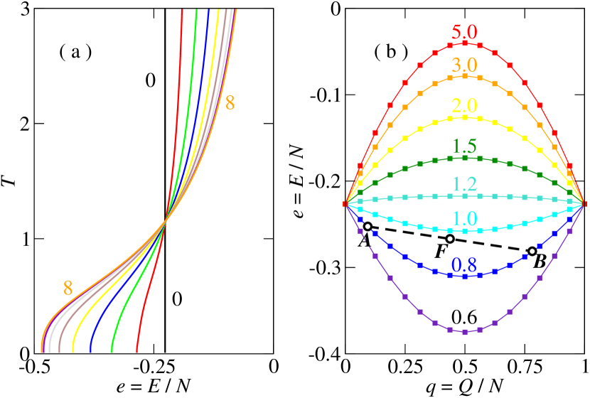
with the partition function . The Boltzmann constant is set to be unity. Figure 2(a) presents the energy-temperature relation in each sector. Also shown in Fig. 2(b) are the isothermal curves. The isotherms have a positive or negative curvature depending on the temperature. The curvature change leads to an intriguing phenomenon, which will be discussed later.
Thermalization — Suppose that the total system is prepared to be in a product state
| (5) |
where and are the eigenstates of and , respectively. The interaction Hamiltonian does not commute with and . Thus, acts as a thermal contact allowing the flows of the energy and the particle. We investigate how the system evolves into the global equilibrium state via the unitary time evolution with . The time evolution is simulated numerically Suzuki (1985) 111See Supplemental Material for more details..
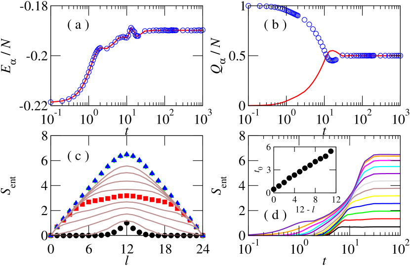
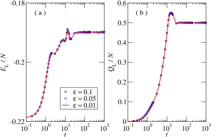
We performed the numerical analysis with the initial state where the subsystem L is empty () and the subsystem is fully occupied (). The expectation values of the energy and the particle number of each subsystem are measured and shown in Fig. 3. After a transient period, the system reaches a stationary state where the energy and the particle are distributed uniformly.
The quantum thermalization is accompanied by the growth of the entanglement entropy Kim and Huse (2013); Kaufman et al. (2016); Nahum et al. (2017). We construct the reduced density operator for the leftmost spins by taking the partial trace over the other spins, and evaluate the entanglement entropy Note (1). The numerical data shown in Fig. 3(c) reveal two distinct transient regimes. The entanglement entropy of the initial product state is identically zero. At short times, the entanglement develops near the contact (). It propagates into the system until deviates from zero at all values of . Afterwards, the entanglement entropy grows and saturates to the stationary profile. Note that the faceted shape with rounded center, i.e., the Page correction, is the typical entanglement entropy profile of a thermal system Page (1993); Nakagawa et al. (2018). The propagation and the growth are clearly seen in Fig. 3(d). We estimate the entanglement propagation speed by measuring the time at which as a function of . It scales linearly with the distance from the boundary. The linear dependence reflects the Lieb-Robinson bound for the quantum information propagation Lieb and Robinson (1972); Hastings and Koma (2006).
We investigate in more detail the property of the steady state. In the presence of , is not the eigenstate of . The energy fluctuation is given by
| (6) |
where . Since is local, the variance is of the order of . The total Hamiltonian satisfies the ETH and the initial state has a finite energy fluctuation. Therefore, the system should thermalize to the equilibrium state in the long time limit.
We characterize the equilibrium state with the probability distribution that the subsystem is in the eigenstate of . It is given by
| (7) |
where is the reduced density matrix of the subsystem . The total system is thermal and can be regarded as the equilibrium heat bath for subsystems. Thus, the subsystem probability is given by
| (8) |
where , , and is the thermodynamic entropy of the subsystem . Here, we assume the weak coupling limit that the interaction energy is negligible.
Let and denote the deviations of the energy and the particle number from their steady state values and . In terms of and , we can approximate (8) as
| (9) |
with the temperature and the chemical potential defined as and . We also keep the quadratic terms with the second order derivatives of the thermodynamic entropy. When the subsystem is much smaller than the total system, it suffices to keep the linear order terms. Then, reduces to the grand canonical ensemble distribution. In the current situation, however, the subsystem size is comparable to the total system size. It is necessary to keep the higher order terms.
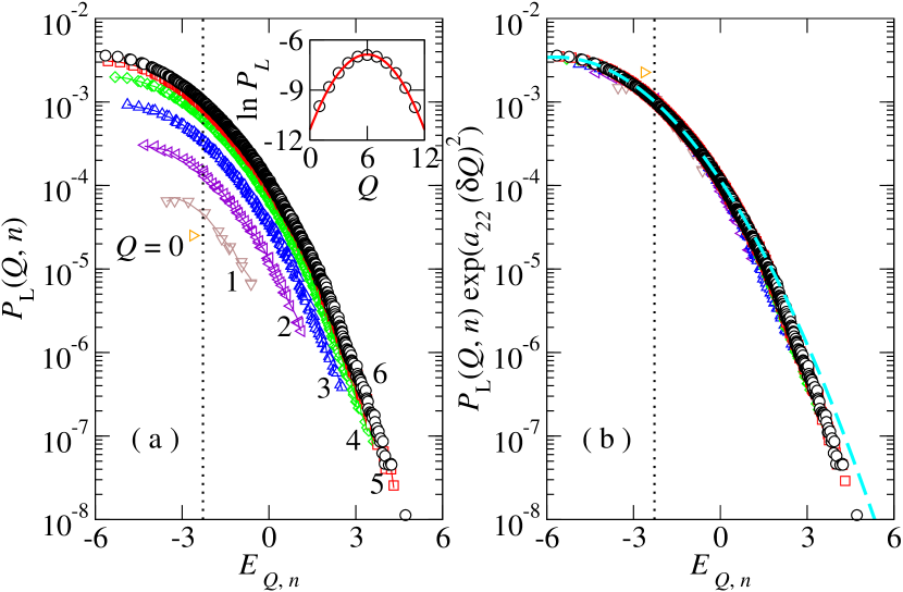
We confirm the equilibrium distribution in (9) numerically. Starting from the same initial condition as in Fig. 3, we constructed the reduced density matrix averaged over the time interval when the system reaches the steady state, and calculated using (7) (see Fig. 4). In the half-filling case (), the system obeys the particle-hole symmetry. Thus, the distribution function takes a simpler form
| (10) |
with . In order to verify the quadratic dependence on , we select the eigenstate whose energy eigenvalue is closest to the average energy at each . The probabilities at these energy levels are plotted in the inset of Fig. 4(a). The quadratic dependence is evident with . We plot the rescaled probability distributions with in Fig. 4(b). They collapse onto a single curve, which is well fitted to the function with and . The data collapse confirms the equilibrium distribution function in (10). One can notice a slight deviation at large values of and , where even higher order corrections are necessary.
Joule expansion — During the thermalization, the quantum gas undergoes the Joule expansion or the free expansion into a vacuum. We discuss the thermodynamic consequence of the Joule expansion.
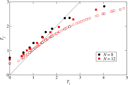
Suppose that the system is prepared in the initial state (5) with and . The subsystem can be in any state with . For an initial state with given , the gas has a definite initial temperature determined from (4). The final temperature after thermalization can be measured by fitting the probability distribution , defined in (7), to the form of (9).
We have performed the numerical analysis with the subsystems of size and and . In fitting, we used the data of the most probable sector where the probability takes the simple form with . The resulting temperature is plotted as a function of in Fig. 5(a). Interestingly, the quantum gas may either heat up or cool down depending on the initial temperature. The two regions are separated by a inversion temperature . We also studied the Joule expansion from a dense region to a dilute (nonempty) region and obtained the similar result Note (1).
Taking it for granted that the system thermalizes, the heating or cooling can be understood easily. Let and be the initial energy density and particle density of the subsystem . After the interaction turns on, the total system has the energy density and the particle density . The correction to the energy density is negligible in the large limit. One may represent the thermodynamic state of the subsystems and the total system in the energy density-particle density plane along with the isotherms (see Fig. 2(b)). In this plane, the total system after expansion is represented by the midpoint of and . The final temperature can be read from the isotherm passing through . We illustrate this construction in Fig. 2(b), where the initial states are marked as and while the final state as . It clearly shows that the gas heats up (cools down) if the isothermal curves are convex (concave). We compare the final temperatures from the isotherms and the probability distributions in Fig. 5(a). A little discrepancy is due to the correction to the energy density.
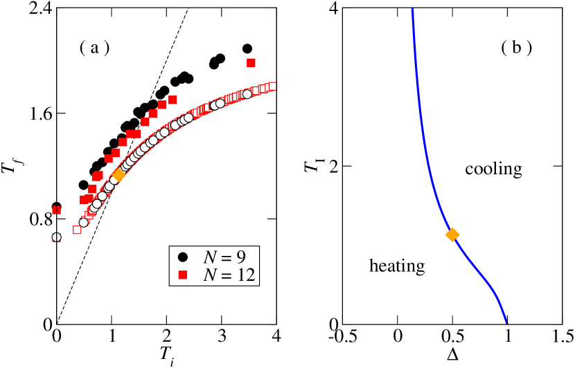
At the inversion temperature , the isotherms change the convexity and the - curves in all sectors cross each other (see Fig. 2(a)). We can locate the inversion temperature under reasonable assumptions: (i) - curves in and sectors cross at . (ii) The periodic boundary condition yields the same result in the limit. Under these assumptions, the inversion temperature is determined by
| (11) |
with Note (1). We evaluate the inversion temperature as a function of . The inversion curve thus-obtained at is presented in Fig. 5(b). It vanishes as near and diverges as near .
The inversion curve has an interesting implication. Suppose that one can perform the Joule expansion repeatedly. Then, the temperature of the gas converges to the inversion temperature for . That is, the inversion temperature is the stable fixed point under the Joule expansion.
The classical gas with the Lennard-Jones potential also has the inversion temperature Goussard and Roulet (1993). The mean field theory shows that the gas heats up above the inversion temperature and cools down below the inversion temperature. Namely, the inversion temperature in the classical regime corresponds to the unstable fixed point under the Joule expansion. The distinct role of the two inversion temperatures manifests that the Joule expansion of the quantum gas is a correlated many-body process.
Summary — We investigated the equilibration of two subsystems of comparable size. They are coupled by an interaction Hamiltonian allowing the flows of energy and particle. Based on the ETH, we derived that the probability distribution of the subsystem follows the grand canonical ensemble distribution with nonlinear corrections. Our setup describes a Joule expansion of a quantum gas. We showed that the quantum gas can be cooled or heated upon expansion with the inversion temperature. The emergent inversion temperature corresponds to the stable fixed point under the Joule expansion. It signals that the Joule expansion of the quantum gas is a correlated many-body process, which requires a thorough investigation beyond the classical mean field theory. We expect that the cooling/heating scenario can be verified using the free expansion experiments of ultracold atom gases. We also expect that the Joule expansion can be useful for the temperature control of quantum gases.
Acknowledgements.
This work was supported by the the National Research Foundation of Korea (NRF) grant funded by the Korea government (MSIP) (No. 2016R1A2B2013972). E.I. and T.S. are supported by JSPS KAKENHI Grand Number JP16H02211. E.I. is also supported by KAKENHI Grant Number JP15K20944.References
- D’Alessio et al. (2016) L. D’Alessio, Y. Kafri, A. Polkovnikov, and M. Rigol, Adv. Phys. 65, 239 (2016).
- Srednicki (1994) M. Srednicki, Phys. Rev. E 50, 888 (1994).
- Deutsch (1991) J. M. Deutsch, Phys. Rev. A 43, 2046 (1991).
- Kim et al. (2014) H. Kim, T. N. Ikeda, and D. A. Huse, Phys. Rev. E 90, 052105 (2014).
- Yoshizawa et al. (2018) T. Yoshizawa, E. Iyoda, and T. Sagawa, Phys. Rev. Lett. 120, 200604 (2018).
- Rigol (2009) M. Rigol, Phys. Rev. Lett. 103, 015101 (2009).
- von Neumann (2010) J. von Neumann, Eur. Phys. J. H 35, 201 (2010).
- Beugeling et al. (2014) W. Beugeling, R. Moessner, and M. Haque, Phys. Rev. E 89, 042112 (2014).
- Jensen and Shankar (1985) R. V. Jensen and R. Shankar, Phys. Rev. Lett. 54, 1879 (1985).
- Rigol et al. (2008) M. Rigol, V. Dunjko, and M. Olshanii, Nature 452, 854 (2008).
- Kinoshita et al. (2006) T. Kinoshita, T. Wenger, and D. S. Weiss, Nature 440, 900 (2006).
- Tang et al. (2018) Y. Tang, W. Kao, K.-Y. Li, S. Seo, K. Mallayya, M. Rigol, S. Gopalakrishnan, and B. L. Lev, Phys. Rev. X 8, 021030 (2018).
- Trotzky et al. (2012) S. Trotzky, Y.-A. Chen, A. Flesch, I. P. McCulloch, U. Schollwöck, J. Eisert, and I. Bloch, Nature Physics 8, 325 (2012).
- Langen et al. (2015) T. Langen, S. Erne, R. Geiger, B. Rauer, T. Schweigler, M. Kuhnert, W. Rohringer, I. E. Mazets, T. Gasenzer, and J. Schmiedmayer, Science 348, 207 (2015).
- Kaufman et al. (2016) A. M. Kaufman, M. E. Tai, A. Lukin, M. Rispoli, R. Schittko, P. M. Preiss, and M. Greiner, Science 353, 794 (2016).
- Kim et al. (2018) H. Kim, Y. Park, K. Kim, H. S. Sim, and J. Ahn, Phys. Rev. Lett. 120, 180502 (2018).
- Neill et al. (2016) C. Neill, P. Roushan, M. Fang, Y. Chen, M. Kolodrubetz, Z. Chen, A. Megrant, R. Barends, B. Campbell, B. Chiaro, A. Dunsworth, E. Jeffrey, J. Kelly, J. Mutus, P. J. J. O’Malley, C. Quintana, D. Sank, A. Vainsencher, J. Wenner, T. C. White, A. Polkovnikov, and J. M. Martinis, Nature Physics 12, 1037 (2016).
- Biroli et al. (2010) G. Biroli, C. Kollath, and A. M. Läuchli, Phys. Rev. Lett. 105, 250401 (2010).
- Imbrie (2016) J. Z. Imbrie, Phys. Rev. Lett. 117, 027201 (2016).
- Turner et al. (2018) C. J. Turner, A. A. Michailidis, D. A. Abanin, M. Serbyn, and Z. Papić, Nature Physics 14, 745 (2018).
- Shiraishi and Mori (2017) N. Shiraishi and T. Mori, Phys. Rev. Lett. 119, 030601 (2017).
- Mondaini et al. (2018) R. Mondaini, K. Mallayya, L. F. Santos, and M. Rigol, Phys. Rev. Lett. 121, 038901 (2018).
- Shiraishi and Mori (2018) N. Shiraishi and T. Mori, Phys. Rev. Lett. 121, 038902 (2018).
- Ponomarev et al. (2011) A. V. Ponomarev, S. Denisov, and P. Hänggi, Phys. Rev. Lett. 106, 010405 (2011).
- Reif (1965) F. Reif, Fundamentals of Statistical and Thermal Physics (McGraw-Hill, New York, 1965).
- Blundell and Blundell (2006) S. J. Blundell and K. M. Blundell, Concepts in Thermal Physics (Oxford University Press, New York, 2006).
- Goussard and Roulet (1993) J. O. Goussard and B. Roulet, Am. J. Phys. 61, 845 (1993).
- Camalet (2008) S. Camalet, Phys. Rev. Lett. 100, 180401 (2008).
- Schneider et al. (2012) U. Schneider, L. Hackermüller, J. P. Ronzheimer, S. Will, S. Braun, T. Best, I. Bloch, E. Demler, S. Mandt, D. Rasch, and A. Rosch, Nature Physics 8, 213 (2012).
- Cazalilla et al. (2011) M. A. Cazalilla, R. Citro, T. Giamarchi, E. Orignac, and M. Rigol, Rev. Mod. Phys. 83, 1405 (2011).
- Santos et al. (2011) L. F. Santos, A. Polkovnikov, and M. Rigol, Phys. Rev. Lett. 107, 040601 (2011).
- Suzuki (1985) M. Suzuki, J. Math. Phys. 26, 601 (1985).
- Note (1) See Supplemental Material for more details.
- Kim and Huse (2013) H. Kim and D. A. Huse, Phys. Rev. Lett. 111, 127205 (2013).
- Nahum et al. (2017) A. Nahum, J. Ruhman, S. Vijay, and J. Haah, Phys. Rev. X 7, 401 (2017).
- Page (1993) D. N. Page, Phys. Rev. Lett. 71, 1291 (1993).
- Nakagawa et al. (2018) Y. O. Nakagawa, M. Watanabe, H. Fujita, and S. Sugiura, Nat. Comm. 9, 1 (2018).
- Lieb and Robinson (1972) E. H. Lieb and D. W. Robinson, Commun. Math. Phys. 28, 251 (1972).
- Hastings and Koma (2006) M. B. Hastings and T. Koma, Commun. Math. Phys. 265, 781 (2006).
I Supplmental material
I.1 Numerical method to solve the Schrödinger equation
The state vector at time is given by with the unitary time evolution operator
| (S1) |
When the whole set of eigenvectors of is available, it is given by with . This is the exact method.

When the dimension of the Hilbert space is too large, the exact method is impractical and one needs to rely on an approximate method. We will explain an efficient method to simulate the time evolution. The XXZ Hamiltonian of spins under the open boundary condition is given by (see Fig. S1)
| (S2) |
with the short-hand notation
| (S3) | ||||
where .
Note that the Hamiltonian is slightly different from that considered in the paper. Generalizations to the Hamiltonian with bond-dependent and are straightforward.
The time evolution operator satisfies . Thus, the state vector at is obtained by multiplying to the initial state vector times repeatedly. For infinitesimal , can be approximated efficiently. First, we decompose the Hamiltonian as the sum with
| (S4) |
In Fig. S1, the interaction bonds contained in , , , and are represented by the solid, dashed, dotted, and dash-dotted lines, respectively. Then, using the generalized Lie-Suzuki-Trotter formula of the second order [30], we obtain
| (S5) |
The important feature of the decomposition (S4) is that all ’s contained in a partial Hamiltonian commute with each others. It yields
| (S6) |
and similar relations for the others. Consequently, can be approximated as the ordered product of with or with an error . If one chooses as the basis states for the spins at sites and , with the unitary matrix
| (S7) |
with . The overall error of this method is of the order of .
Computationally, the infinitesimal time evolution is achieved by the multiplication of a state vector with the matrices times. All the operators ’s conserve the total number of up spins. Thus, one can work within the subspace consistent with the conservation, which make numerical calculations efficient. In the numerical calculations, we used the exact time evolution when , and the decomposition method for with . We examined whether is small enough. As can be seen in Fig. S2, the data with , and are indistinguishable in the plot. More quantitatively, the values of at time are , , and for , , and , respectively. They are well fitted to the function with . The relative error of the value at is . It proves that is small enough.
I.2 Singular value decomposition for reduced density matrix
Suppose that one separates the spins into two sets of spins and of spins. We assume that without loss of generality. Then, the state vector can be written as
| (S8) |
where and span the Hilbert spaces of dimension and for spins in and , respectively. The reduced density operator for the spins in is given by
| (S9) |
and represented by the reduced density matrix is given by
| (S10) |
The reduced density matrix is necessary when one calculates the local observables and the probability distribution for the spins in . The eigenvalues are necessary for the entanglement entropy. The singular value decomposition (SVD) is a convenient method to handle the reduced density matrix.
The probability amplitudes can be regarded as the elements of a positive semidefinite complex matrix , . According to the SVD, such a matrix can be written as
| (S11) |
where is a unitary matrix, is a rectangular diagonal matrix with non-negative real diagonal elements, and is a unitary matrix. The SVD can be done with a numerical analysis software.
Once the SVD is done, the reduced density matrix is obtained from the relation
| (S12) |
That is, the reduced density matrix is given by the similarity transformation of the diagonal matrix
| (S13) |
The SVD allows one to calculate the entanglement entropy easily. It is given by
| (S14) |
I.3 Temperature-energy relation in the sector
Consider the XXZ Hamiltonian of spins under the periodic boundary condition. In the sector where all spins are down (or all sites are empty), there is a single eigenstate with the energy
| (S15) |
The Hilbert space of the sector is spanned by the states where represents the state where the particle is at site . The plane wave is the eigenstate and the energy eigenvalue is given by
| (S16) |
with (). The partition function in the sector is given by
| (S17) |
with the mean energy
| (S18) |
We estimate the location of the inversion temperature by requiring that the mean energy in the sector should be equal to the energy in the section. It yields that
| (S19) |
with . In the limit, the summation is replaced by the integration to yield the expression
| (S20) |
Note that increases as or . For small , we can approximate
| (S21) |
Thus, the inversion temperature has the limit form
| (S22) |
as . In the opposite limit where (), is dominated by the minimum value of . For positive , takes the minimum value at . It yields that .
I.4 Joule expansion
In the main text, we present the Joule expansion of a gas into the vacuum. We have performed the numerical simulation of the Joule expansion in a mixture of a dense gas and a dilute gas. The subsystems and is prepared in the energy eigenstates and , respectively, with and with the same quantum number . The two states are tied to each other by the particle-hole symmetry. We select those two states in order to keep them in the same initial temperature.
When the total system reaches a stationary state, we measure the probability distribution that the subsystem is in the state . Then, we fit the probability distribution to the function at the most probable sector to find the final temperature . The numerical result is presented in Fig. S3. We also observe that the gas heats up (cools down) when the initial temperature is lower (higher) than a threshold temperature. The finite size effect is also seen in the plot.