Generalized Dynamic Factor Models and Volatilities:
Consistency, Rates, and Prediction Intervals

Abstract

Volatilities, in high-dimensional panels of economic time series with a dynamic factor structure on the levels or returns, typically also admit a dynamic factor decomposition. We consider a two-stage dynamic factor model method recovering the common and idiosyncratic components of both levels and log-volatilities. Specifically, in a first estimation step, we extract the common and idiosyncratic shocks for the levels, from which a log-volatility proxy is computed. In a second step, we estimate a dynamic factor model, which is equivalent to a multiplicative factor structure for volatilities, for the log-volatility panel. By exploiting this two-stage factor approach, we build one-step-ahead conditional prediction intervals for large $n\times T$ panels of returns. Those intervals are based on empirical quantiles, not on conditional variances; they can be either equal- or unequal-tailed. We provide uniform consistency and consistency rates results for the proposed estimators as both $n$ and $T$ tend to infinity. We study the finite-sample properties of our estimators by means of Monte Carlo simulations. Finally, we apply our methodology to a panel of asset returns belonging to the S&P100 index in order to compute one-step-ahead conditional prediction intervals for the period 2006-2013. A comparison with the componentwise GARCH benchmark (which does not take advantage of cross-sectional information) demonstrates the superiority of our approach, which is genuinely multivariate (and high-dimensional), nonparametric, and model-free.

JEL Classification: C32, C38, C58.
Keywords: Volatility, Dynamic Factor Models, Prediction intervals, GARCH.

1 Introduction

Data in high dimension unquestionably constitute one of the main challenges of contemporary statistics/econometrics, and have become pervasive in most domains related with data sciences. Time series have not escaped that evolution, and the analysis of high-dimensional time series—equivalently, large cross-sections of univariate time series or panels—today ranks among the most active topics in theoretical and applied econometrics.

The most successful methods so far in the analysis and prediction of high-dimensional time series are based on the so-called factor model approach. That approach, under its various forms, is based on a (non-observed) decomposition of the observation (a large cross-section of time series with complex interrelations) into the sum of two mutually orthogonal (all leads, all lags) components: the common component, driven by a small number of factors or common shocks, and an idiosyncratic component, with some variations in the definitions of “common” and “idiosyncratic,” and the assumptions made. Regardless of the definition adopted, the common and idiosyncratic components typically are disentangled by means of adequate cross-sectional and/or temporal aggregation of the observed time series.

Those aggregation and factor model approaches are strongly rooted in the multivariate time-series methods developed in the eighties and nineties, of which George Tiao and his collaborators have been most influential and unremittable pioneers: see, for instance, Tiao, (1972), Tiao and Hillmer, (1978), Tiao and Guttman, (1980), Tiao and Box, (1981), Tsay and Tiao, (1985), Peña and Box, (1987), and Tiao and Tsay, (1989).

The type of factor model we are considering here is the General or Generalized Dynamic Factor Model (GDFM) introduced by Forni et al., (2000), which, by taking into account all leading and lagging linear dependencies among the data, encompasses most other models, as e.g. the static factor approaches by Bai and Ng, (2002), Stock and Watson, (2002), and Fan et al., (2013). Moreover, as emphasised in Forni and Lippi, (2001) and Hallin and Lippi, (2013), beyond the usual assumptions of second-order stationarity and existence of spectral densities, the GDFM decomposition into a common and an idiosyncratic component basically does not place any structural constraints on the data-generating process. In this sense, contrary to static factor approaches, it is canonical, nonparametric and model-free. In this paper, we consider the one-sided GDFM estimation method recently described in Forni et al., (2015, 2017).

Prediction, in classical univariate and moderately multivariate time series analysis, is an obvious and natural objective; it is certainly no less crucial in high dimension. Efficient prediction, however, should exploit the amount of information available, due to the complex cross-dependencies among the many cross-sectional components, in the present and lagged values of the whole cross-section; the larger the cross-section (i.e., the higher the dimension), the more crucial the role of that information, and the more delicate its recovering. Factor models naturally have been used in the construction of point-predictors, and quite successfully so: see, e.g., Stock and Watson, (2002), Bai and Ng, (2008), Forni et al., (2018), to quote only a very few. Those authors, however, are dealing, mostly, with macroeconomic data, while less attention has been given to factor model methods in the analysis and prediction of financial returns: see, e.g. Chamberlain and Rothschild, (1983), Connor and Korajczyk, (1993), or Aït-Sahalia and Xiu, (2017). In particular, when dealing with returns, due to the presence of conditional distribution heterogeneity (of which conditional heteroskedasticity is only a very particular case), conditional volatility phenomenons are essential, and definitely should be taken into account when building conditional prediction limits or conditional prediction intervals.

Most multivariate methods available in the literature for the analysis of conditional heterogeneity are restricted to the study of conditional heteroskedasticity, and rely on parametrisations of the ARCH-GARCH or Stochastic Volatility type: see, for instance, the reviews by Bauwens et al., (2006) and Asai et al., (2006). Because of the curse of dimensionality, however, only the very simplest models can be considered in high-dimensional panels, possibly inducing a nonnegligible loss of efficiency. Among those, the factor GARCH approach is the most popular, see e.g. Diebold and Nerlove, (1989), Ng et al., (1992), Harvey et al., (1992), and Sentana et al., (2008). Static factor models directly based on volatilities have also been considered, but these fail to exploit the information contained in the idiosyncratic components of returns, see e.g. Connor et al., (2006) and Fan et al., (2015). For these reasons, Barigozzi and Hallin, (2016) introduce a two-step GDFM approach by which the nonparametric and model-free virtues of factor models are used in a joint analysis of returns and volatilities. In Barigozzi and Hallin, 2017a , that two-step GDFM is combined with a GARCH strategy in order to produce point-forecasts for volatilities (see also Trucíos et al., , 2019 for a recent example), while Barigozzi and Hallin, 2017b and Barigozzi et al., (2018) apply the same methodology in a study of the dynamic interdependencies of US and international financial markets. A two-stage factor approach similar to ours but in a static factor model setting is proposed in Chicheportiche and Bouchaud, (2015).

The objective of this paper is to combine the same two-step GDFM approach with a quantile-based construction of conditional confidence limits producing conditional interval predictions rather than point-forecasts for returns. That objective requires nontrivial consistency results on the two-step GDFM estimation method, which are not provided in Barigozzi and Hallin, (2016); Barigozzi and Hallin, 2017a ; Barigozzi and Hallin, 2017b . The first part of this paper, therefore, is devoted to a careful asymptotic analysis of the two-step GDFM. We then describe the quantile-based construction of conditional confidence limits, which we apply to a dataset of S&P100 daily returns.

The paper is organised as follows. In Section 2, we present the GDFM model for the stochastic processes of returns (levels) and log-volatilities, and give sufficient conditions for its existence and identification. Section 3.1 describes the estimation of the model, and Section 3.2 establishes the consistency properties (with rates) of the proposed estimators. In Section 4, we define the one-step-ahead conditional prediction confidence limits and intervals. In Section 5, we study the finite-sample properties of our estimators via simulations. Section 6 applies our methodology to a panel of daily returns of stocks listed in the S&P100 index and investigates the resulting coverage performance. In Section 7, we conclude. Proofs are postponed to an Appendix.

Notation

The sub-exponential norm of a scalar random variable $X$ is defined as $\|X\|_{\psi_{1}}:=\sup_{p\geq 1}p^{-1}\mathrm{E}[|X|^{p}]^{1/p}$ (see e.g. Definition 5.13 in Vershynin, , 2012). The transposed complex conjugate of a complex vector $\bf p$ is denoted as ${\bf p}^{\dagger}$ and $\|\bf p\|=\bf p^{\dagger}\bf p$. For an hermitian complex $n\times n$ matrix $\mathbf{A}$ with generic $(i,j)$ entry $a_{ij}$ and largest (in modulus) eigenvalue $\mu^{\mathbf{A}}_{1}$, let $\|\mathbf{A}\|_{1}:=\max_{j=1,\ldots,n}\sum_{i=1}^{n}|a_{ij}|$ and $\|\mathbf{A}\|:={\mu_{1}^{\mathbf{A}}}$. As usual, $L$ stands for the lag operator, such that, given a stochastic vector process $\{\mathbf{Y}_{t}|t\in\mathbb{Z}\}$, $L^{k}\mathbf{Y}_{t}:=\mathbf{Y}_{t-k}$ for any integer $k$ and any $t\in\mathbb{Z}$. Last, we denote by $\mathbb{I}(\mathcal{A})$ the indicator function of an event $\mathcal{A}$.

2 A General Dynamic Factor Model for levels and volatilities

We throughout assume that all stochastic variables in this paper belong to the Hilbert space $L_{2}(\Omega,\mathcal{F},\mathrm{P})$, where $(\Omega,\mathcal{F},\mathrm{P})$ is some common probability space. We study double-indexed stochastic processes of theform $\mathbf{Y}\!:=\{Y_{it}|i\in\mathbb{N},\ t\in\mathbb{Z}\}$, with $n$-dimensional sub-processes $\mathbf{Y}_{n}\!:=\{Y_{it}|i=\leavevmode\nobreak\ \!1,\ldots,n,\leavevmode\nobreak\ t\in\leavevmode\nobreak\ \!\mathbb{Z}\}$, $n\in\mathbb{N}$. In practice, we deal with the finite observed $n\times T$ realisation

$${\bf Y}_{n,T}:=\left(\begin{array}[]{cccc}Y_{11},&Y_{12},&\ldots,&Y_{1T}\\ \vdots&\vdots&&\vdots\\ Y_{n1},&Y_{n2},&\ldots,&Y_{nT}\end{array}\right)$$

of $\mathbf{Y}$. In the empirical application of Section 6, the $Y_{it}$’s are observed values of daily stock returns, and we therefore call $\mathbf{Y}$ the “levels” process. The assumptions in Section 2.1 are mainly taken from Forni et al., (2017), with some modifications, mostly concerning the idiosyncratic components. On the other hand, the assumptions in Section 2.2 are new and are related to the log-volatility proxies originally introduced in Barigozzi and Hallin, (2016); Barigozzi and Hallin, 2017a .

2.1 Model and assumptions for levels

The Generalized Dynamic Factor Model (GDFM) for the levels process $\mathbf{Y}$ is a decomposition of $Y_{it}$ into

$$Y_{it}-\mathrm{E}[Y_{it}]=X_{it}+Z_{it},\quad i\in\mathbb{N},\ t\in\mathbb{Z}$$ (2.1)

with

$$X_{it}=\sum_{j=1}^{q}\sum_{k=0}^{\infty}b_{ijk}u_{jt-k}=\mathbf{b}_{i}^{\prime}(L)\mathbf{u}_{t}\quad\text{and}\quad Z_{it}=\sum_{k=0}^{\infty}d_{ik}v_{it-k}=d_{i}(L)v_{it},$$ (2.2)

where $\mathrm{E}[Y_{it}]$ stands for the expected value of $Y_{it}$ and the processes $\mathbf{u}:=\{u_{jt}|j=1,\ldots,q,\ t\in\mathbb{Z}\}$ and $\mathbf{v}_{n}:=\{v_{it}|i=1,\ldots,n,\ t\in\mathbb{Z}\}$ are mutually orthogonal (at all leads and lags) $q$- and $n$-dimensional white noises, respectively. Call $\mathbf{u}$ the process of common factors or common shocks and $\mathbf{v}_{n}$ the process of idiosyncratic shocks; $X_{it}$ and $Z_{it}$ are $Y_{it}$’s common and idiosyncratic components, respectively.

Letting $\mathbf{X}_{n}:=\{X_{it}|i=1,\ldots,n,\ t\in\mathbb{Z}\}$ and $\mathbf{Z}_{n}:=\{Z_{it}|i=1,\ldots,n,\ t\in\mathbb{Z}\}$, equations (2.2) in vector notation takes the form

$$\mathbf{X}_{nt}=\mathbf{B}_{n}(L)\mathbf{u}_{t},\qquad\mathbf{Z}_{nt}=\mathbf{D}_{n}(L)\mathbf{v}_{nt},\quad n\in\mathbb{N},\ t\in\mathbb{Z}.$$ (2.3)

with $\mathbf{B}_{n}(L):=(\mathbf{b}_{1}(L)\ldots\mathbf{b}_{n}(L))^{\prime}$, and $\mathbf{D}_{n}(L):=\text{\rm diag}(d_{1}(L)\ldots d_{n}(L))$.

More precisely, we assume that (2.1)-(2.2) hold and satisfy the following assumptions:

Assumption (L1).

 

1. the dimension $q$ of $\mathbf{u}_{t}$ does not depend on $n$; the process $\mathbf{u}:=\{\mathbf{u}_{t}|t\in\mathbb{Z}\}$ is second-order white noise, with mean $\mathbf{0}_{q}$ and diagonal positive definite covariance $\bm{\Gamma}^{\rm u}$;

2. writing ${\mathbf{b}}_{ik}:=(b_{i1k}\ldots b_{iqk})^{\prime}$ for the $q\times 1$ coefficient of $L^{k}$ in ${\mathbf{b}}_{i}(L)$, there exists a constant $M_{1}>0$ such that $\sum_{k=0}^{\infty}\|\mathbf{b}_{ik}\|\,|k|\leq M_{1}$ for all $i\in\mathbb{N}$;

3. the process $\mathbf{v}:=\{\mathbf{v}_{nt}|t\in\mathbb{Z}\}$ is second-order white noise, with mean $\mathbf{0}_{n}$ and positive definite covariance $\bm{\Gamma}_{n}^{\rm v}$; moreover, $\mathrm{E}[v_{it}|v_{is}]=0$ for all $i\in\mathbb{N}$ and $t,s\in\mathbb{Z}$ such that $t>s$;

4. there exists a constant $C_{\rm v}>0$ such that $\|\bm{\Gamma}_{n}^{\rm v}\|_{1}\leq C_{\rm v}$ for all $n\in\mathbb{N}$;

5. there exists a constant $M_{2}>0$ such that $\sum_{k=0}^{\infty}|d_{ik}|\,|k|\leq M_{2}$ for all $i\in\mathbb{N}$;

6. $\text{\rm Cov}(u_{jt},v_{is})=0$ for all $i\in\mathbb{N}$, $j=1,\ldots,q$, and $t,s\in\mathbb{Z}$;

7. there exists a constant $M_{3}>0$ such that $\sum_{k_{1},k_{2},k_{3}\in\mathbb{Z}}\big{|}\mathrm{E}[u_{j_{1}t}u_{j_{2},t-k_{1}}u_{j_{3},t-k_{2}}u_{j_{4},t-k_{3}}]\big{|}\leq M_{3}$ for all $j_{1},j_{2},j_{3},j_{4}=1,\ldots,q$;

8. there exists a constant $M_{4}>0$ such that $\sum_{k_{1},k_{2},k_{3}\in\mathbb{Z}}\big{|}\mathrm{E}[v_{i_{1}t}v_{i_{2},t-k_{1}}v_{i_{3},t-k_{2}}v_{i_{4},t-k_{3}}]\big{|}\leq M_{4}$ for all$i_{1},i_{2},i_{3},i_{4}\in\mathbb{N}$.

These assumptions are standard in the literature with the exception of part (iv) which imposes a mild form of sparsity on the covariance matrix of the idiosyncratic innovations. A similar condition can be found in Fan et al., (2013) and is empirically verified by Boivin and Ng, (2006) and Bai and Ng, (2008) for US macroeconomic data, and by Barigozzi and Hallin, 2017b for stock returns. As a consequence of parts (iv) and (v), the idiosyncratic components are allowed to be serially autocorrelated and mildly cross-correlated (see also Lemma 1 below). Moreover, it is easy to check that such assumption is nesting other typical conditions on the cross-sectional dependence of idiosyncratic components (see e.g. Bai and Ng, , 2002, and Stock and Watson, , 2002, in the static factor model case). Parts (ii) and (v) imply absolute summability of the autocovariances and therefore the existence of a purely continuous spectral density. Moreover these assumptions and existence of fourth-order moments in parts (vii) and (viii) are classical requirements for consistent estimation of the autocovariances and the spectral density (see e.g. Chapter IV, Theorem 6, in Hannan, , 1970, for the autocovariances, and the results in Section 6.2 in Priestley, , 2001, and Theorem 5A in Parzen, , 1957, for the spectral density). Last, in part (iii) we also make the typical assumption of martingale difference innovations used in the GARCH literature (see e.g. Definition 2.1 in Francq and Zakoian, , 2011).

It should be insisted, however, that the GDFM is not a statistical model in the usual sense, inasmuch as, beyond the requirement of second-order stationarity, the existence of a finite (but unspecified) $q$, and the existence of a spectrum, it does not really impose any restrictions on the data-generating process: as argued by Forni and Lippi, (2001) and Hallin and Lippi, (2013), (2.1)-(2.2) indeed constitute a representation result rather than a model equation.

On the filters $\mathbf{b}_{i}(L)$ and $d_{i}(L)$ we furthermore impose the following assumptions:

Assumption (L2).

 

1. $\mathbf{b}_{i}(L)$ has rational entries, i.e. $b_{ij}(L)=\theta_{ij}(L)\phi^{-1}_{ij}(L)$, where $\phi_{ij}(z)$ and $\theta_{ij}(z)$, for all $i\in\mathbb{N}$ and $j=1,\ldots,q$, are finite-order polynomials;

2. there exists a constant $\bar{\phi}>1$ such that $\phi_{ij}(z)\neq 0$ for all $i\in\mathbb{N}$, all $j=1,\ldots,q$, and all $z\in\mathbb{C}$ such that $|z|\leq\bar{\phi}$;

3. the coefficients $\theta_{ijk}$ of $\theta_{ij}(L)$ are such that $|\theta_{ijk}|\leq B^{X}$ for some positive constant $B^{X}$, all $k\in\mathbb{N}\cup\{0\}$, all $i\in\mathbb{N}$, and $j=1,\ldots,q$;

4. $d_{i}(L)$ is of the form $c_{i}^{-1}(L)$ where $c_{i}(z)$, for all $i\in\mathbb{N}$, is a finite-order polynomial, $c_{i}(0)=1$ and $c_{i}(z)\neq 0$ for all $z\in\mathbb{C}$ such that $|z|\leq 1$.

This latter assumption is not strictly needed and could be easily relaxed to allow for infinite order autoregressive dynamics—at the expense, however, of heavier notation and longer proofs; see also Section 3.2 for a short discussion. This assumption implies that both the common and idiosyncratic components have a rational spectral density. Rational filters for the common component are also assumed in Forni et al., (2017), while here we also assume that the idiosyncratic component admits a finite autoregressive representation. In particular, using part (iv), we can rewrite the second equation in (2.2) as

$$c_{i}(L)Z_{it}=v_{it}.$$ (2.4)

Let $\bm{\Sigma}_{n}^{Y}(\theta)$, $\bm{\Sigma}_{n}^{X}(\theta)$ and $\bm{\Sigma}_{n}^{Z}(\theta)$, $\theta\in[-\pi,\pi]$, be the $n\times n$ spectral density matrices of the observed panel, the common, and the idiosyncratic components, respectively; the existence of those spectral densities is guaranteed by Assumption (L1). Denote by $\lambda_{nj}^{Y}(\theta)$, $\lambda_{nj}^{X}(\theta)$, and $\lambda_{nj}^{Z}(\theta)$ their respective $j$-th largest eigenvalues—the panel, common, and idiosyncratic dynamic eigenvalues, on which we assume the following. Hereafter, “forall $\theta\in[-\pi,\pi]$” or “$\theta-a.e.$” is to be understood as “for all $\theta$ but over a subset of values included in a set with Lebesgue measure zero.” Similarly, $\sup_{\theta\in[-\pi,\pi]}$ in the sequel is an essential $\sup$, etc.

Assumption (L3).

There exist a positive integer $\bar{n}$ and continuous functions $\alpha_{j}$ and $\beta_{j-1}$ from $[-\pi,\pi]$ to $\mathbb{R}\,$, $j=1,\ldots,q$, independent of $n$, and such that

$$0<\beta_{j-1}(\theta)<\alpha_{j}(\theta)\leq{\lambda_{nj}^{X}(\theta)}/{n}\leq\beta_{j}(\theta)<\infty\quad\!\!\text{ $\theta$-a.e. in $[-\pi,\pi]$, all $j=1,\ldots,q$, and all $n>\bar{n}$. }$$

Under this assumption, the first $q$ common dynamic eigenvalues, irrespective of the frequency $\theta$ (except possibly over a set of measure zero), are diverging linearly as $n\to\leavevmode\nobreak\ \!\infty$. The following results then hold for the idiosyncratic dynamic eigenvalues and those of the panel.

Lemma 1.

Under Assumptions (L1) and (L3),

1. there exists a constant $C^{Z}>0$ such that $\sup_{\theta\in[-\pi,\pi]}\lambda_{n1}^{Z}(\theta)\leq C^{Z}$ for all $n\in\mathbb{N}$;

2. there exist a positive integer $\bar{n}$ and continuous functions $\alpha_{j}^{Y}$ and $\beta_{j-1}^{Y}$ from $[-\pi,\pi]$ to $\mathbb{R}\,$,$j=1,\ldots,q$, independent of $n$ and such that $0<\beta_{j-1}^{Y}(\theta)<\alpha_{j}^{Y}(\theta)\leq{\lambda_{nj}^{Y}(\theta)}/{n}\leq\beta_{j}^{Y}(\theta)\!<\infty$, $\theta$-a.e. in $[-\pi,\pi]$, all $j=1,\ldots,q$, and all $n>\bar{n}$;

3. there exists a constant $C^{Y}>0$ such that $\sup_{\theta\in[-\pi,\pi]}\lambda_{n,q+1}^{Y}(\theta)\leq C^{Y}$ for all $n\in\mathbb{N}$.

As a consequence of Lemma 1, identification of the model, i.e., consistently disentangling the unobserved common and idiosyncratic components, is possible, under the assumptions made in the limit, as $n\to\infty$, thanks to the behaviour of the dynamic eigenvalues.

Based on results by Anderson and Deistler, (2008) for singular vector processes with a rational spectrum, Forni and Lippi, (2011) and Forni et al., (2015) prove that, for generic values of the coefficients of the filters $\mathbf{b}_{i}(L)$ as defined in Assumption (L2), the space spanned by $u_{j,t-k}$ for $j=1,\ldots,q$ and $k\geq 0$ is the same as the space spanned by any $(q+1)$-dimensional subvector of $\mathbf{X}_{t}$ and its lags; moreover, those subvectors admit an autoregressive representation driven by the common shocks ${\bf u}_{t}$.

More precisely, any $(q+1)$-dimensional subvector $\mathbf{X}^{\ddagger}_{t}$ of ${\mathbf{X}}_{nt}$ admits an autoregressive representation of the form

$$\mathbf{A}^{\ddagger}(L)\mathbf{X}^{\ddagger}_{t}=\mathbf{H}^{\ddagger}\mathbf{u}_{t},$$ (2.5)

where $\mathbf{A}^{\ddagger}(L)$ is a finite-order VAR operator such that $\mathbf{A}^{\ddagger}(0)=\mathbf{I}_{q+1}$, $\mathbf{u}_{t}$ is the vector of common shocks in (2.3), and $\mathbf{H}^{\ddagger}$ an appropriate $(q+1)\times q$ matrix. On that representation, we make the following assumptions.

Assumption (L4).

Let $\mathbf{X}^{\ddagger}_{t}$ be an arbitrary $(q+1)$-dimensional subvector of ${\mathbf{X}}_{nt}$: the autoregressive representation (2.5) is such that

1. $\mathbf{A}^{\ddagger}(L)$ is uniquely defined;

2. the degree $S^{\ddagger}$ of $\mathbf{A}^{\ddagger}(z)$ is uniformly bounded, that is, $S^{\ddagger}\leq S$ for some integer $S>0$ independent of $n$ and the choice of the subvector ${\mathbf{X}}^{\ddagger}_{t}$;

3. $\text{\rm det}[\mathbf{A}^{\ddagger}(z)]\neq 0$ for all $z\in\mathbb{C}$ such that $|z|\leq 1$;

4. $\mathbf{H}^{\ddagger}$ is $(q+1)\times q$, with full rank $q$;

5. denoting by $\bm{\Gamma}_{h}^{X^{\ddagger}}$ the lag-$h$ autocovariances of $\mathbf{X}^{\ddagger}:=\{\mathbf{X}^{\ddagger}_{t}|t\in\mathbb{Z}\}$ and defining

   $$\bm{\mathcal{C}}^{\ddagger}:=\left[\begin{array}[]{cccc}\bm{\Gamma}_{0}^{X^{\ddagger}}&\bm{\Gamma}_{1}^{X^{\ddagger}}&\cdots&\bm{\Gamma}_{S-1}^{X^{\ddagger}}\\ \bm{\Gamma}_{-1}^{X^{\ddagger}}&\bm{\Gamma}_{0}^{X^{\ddagger}}&\cdots&\bm{\Gamma}_{S-2}^{X^{\ddagger}}\\ \vdots&\vdots&\ddots&\vdots\\ \bm{\Gamma}_{-S+1}^{X^{\ddagger}}&\bm{\Gamma}_{-S+2}^{X^{\ddagger}}&\cdots&\bm{\Gamma}_{0}^{X^{\ddagger}}\\ \end{array}\right],$$

   $\text{\rm det}(\bm{\mathcal{C}}^{\ddagger})>d>0$, where $d$ is independent of the choice of the subvector ${\mathbf{X}}^{\ddagger}_{t}$.

This assumption allows us to derive an alternative representation of the GDFM (2.2) which is particularly useful for estimation and for the construction, in Section 2.2 below, of a further GDFM for log-volatilities. Without loss of generality, let $n$ factorise into $n=m(q+1)$ for some positive integer $m$, so that we can partition ${\mathbf{X}}_{n}$ into $m$ subprocesses, each of dimension $(q+1)$, of the form ${\mathbf{X}}^{(k)}_{t}:=(X_{(k-1)(q+1),t}\ldots X_{k(q+1)-1,t})^{\prime}$, $k=1,\ldots,m$, with superscript ^(k) substituted for ^‡. Each ${\mathbf{X}}^{(k)}$ satisfies (2.5) and Assumption (L4). Defining the $n\times q$ matrix $\mathbf{H}_{n}:=(\mathbf{H}^{(k)^{\prime}}\cdots\mathbf{H}^{(m)^{\prime}})^{\prime}$, we thus have the VAR representation

$$\mathbf{A}_{n}(L)\mathbf{X}_{nt}=\mathbf{H}_{n}\mathbf{u}_{t},$$ (2.6)

where $\mathbf{A}_{n}(L)$ is $n\times n$ block-diagonal with diagonal blocks $\mathbf{A}^{(1)}(L),\ldots,\mathbf{A}^{(m)}(L)$. Moreover, in view of (2.3), we have $\left[\mathbf{A}_{n}(L)\right]^{-1}\mathbf{H}_{n}=\mathbf{B}_{n}(L)$ (see Proposition 3 in Forni et al., , 2017). Then, the following alternative and equivalent representation of the GDFM holds:

$$\mathbf{A}_{n}(L)\left\{\mathbf{Y}_{nt}-\mathrm{E}[\mathbf{Y}_{nt}]\right\}=\mathbf{H}_{n}\mathbf{u}_{t}+\mathbf{A}_{n}(L)\mathbf{Z}_{n}.$$ (2.7)

The advantage of this representation is that it is “static” in the sense that the common shocks $\mathbf{u}$ now are loaded only contemporaneously and not via filters as in (2.3).

To conclude with, note that the Yule-Walker equations

$$\big{(}\mathbf{A}_{1}^{\ddagger}\cdots\mathbf{A}_{S}^{\ddagger}\big{)}=\big{(}\bm{\Gamma}_{1}^{X^{\ddagger}}\cdots\bm{\Gamma}_{S}^{X^{\ddagger}}\big{)}\big{[}\bm{\mathcal{C}}^{\ddagger}\big{]}^{-1},$$ (2.8)

characterising the $S$ matrix coefficients of $\mathbf{A}^{\ddagger}(L)$ in (2.14) are well defined in view of part (v) of Assumption (L4); the same conclusion holds, blockwise, for the $n$ -dimensional VAR (2.6).

For ease of notation, define the filtered processes

$${\mathbf{Y}}_{n}^{*}:=\mathbf{A}_{n}(L)\left\{\mathbf{Y}_{n}-\mathrm{E}[\mathbf{Y}_{n}]\right\},\quad{\mathbf{X}}^{*}_{n}:=\mathbf{A}_{n}(L)\mathbf{X}_{n},\quad\text{and}\quad{\mathbf{Z}}^{*}_{n}:=\mathbf{A}_{n}(L)\mathbf{Z}_{n}$$

with traditional (static) covariance eigenvalues $\mu_{nj}^{Y^{*}}$, $\mu_{nj}^{X^{*}}$, and $\mu_{nj}^{Z^{*}}$, respectively. Since (2.7) is a static factor model, it is natural to make the following assumption on the eigenvalues of the covariance of ${\mathbf{X}}_{n}^{*}$ (see Assumption 4 in Forni et al., , 2009 or Assumption 6 in Forni et al., , 2017). Unless $q=1$, indeed, it does not even follow from Assumption (L3) that $\mathrm{E}({\mathbf{X}}_{n}^{*}{\mathbf{X}}_{n}^{*\prime})$ has rank $q$.

Assumption (L5).

There exist a positive integer $\bar{n}$ and constants $a_{j}>b_{j-1}$, $j=1,\ldots,q$, independent of $n$ such that $0<a_{j}\leq{\mu_{nj}^{X^{*}}}/{n}\leq b_{j}<\infty$ for all $j=1,\ldots,q$ and all $n>\bar{n}$.

The following results then hold for the eigenvalues $\mu_{nj}^{Z^{*}}$ and $\mu_{nj}^{Y^{*}}$ of the covariance matrices of ${\mathbf{Z}}^{*}_{n}$ and ${\mathbf{Y}}^{*}_{n}$, respectively.

Lemma 2.

Under Assumptions (L1), (L3), (L4), and (L5),

1. there exists a constant $C^{Z^{*}}>0$ such that $\mu_{n1}^{Z^{*}}\leq C^{Z^{*}}$ for all $n\in\mathbb{N}$;

2. there exist a positive integer $\bar{n}$ and constants $a_{j}^{Y^{*}}>b_{j-1}^{Y^{*}}$, $j=1,\ldots,q$, independent of $n$ such that $0<a_{j}^{Y^{*}}\leq{\mu_{nj}^{Y^{*}}}/{n}\leq b_{j}^{Y^{*}}<\infty$ for all $j=1,\ldots,q$ and all $n>\bar{n}$;

3. there exists a constant $C^{Y^{*}}>0$ such that $\mu_{n,q+1}^{Y^{*}}\leq C^{Y^{*}}$ for all $n\in\mathbb{N}$.

2.2 Model and assumptions for volatilities

We define the vector of common innovations (at time $t$) as the $n$-dimensional vector

$$\mathbf{e}_{nt}:=(e_{1t},\ldots,e_{nt})^{\prime}:=\mathbf{H}_{n}\mathbf{u}_{t};$$

for $n>q$, the processes ${\mathbf{e}}_{n}:=\{\mathbf{e}_{nt}|t\in\mathbb{Z}\}$, $n\in\mathbb{N}$ clearly are singular. Then, letting $s_{it}:=e_{it}+v_{it}$, our log-volatility proxy is

$$h_{it}:=\log s_{it}^{2}=\log(e_{it}+v_{it})^{2},$$ (2.9)

yielding the double-indexed stochastic process $\mathbf{h}:=\{h_{it}|i\in\mathbb{N},\ t\in\mathbb{Z}\}$, with $n$-dimensional sub-processes $\mathbf{h}_{n}:=\{h_{it}|i=1,\ldots,n,\ t\in\mathbb{Z}\}$. We call $\mathbf{h}$ the “log-volatilities” process. Similar definitions are used in Engle and Marcucci, (2006) and our previous work (Barigozzi and Hallin, , 2016; Barigozzi and Hallin, 2017a, ; Barigozzi and Hallin, 2017b, , and Barigozzi et al., , 2018). In order for such processes to be well defined we make the following assumption.

Assumption (V0).

For all $i\in\mathbb{N}$ and $t\in\mathbb{Z}$, $|s_{it}|>0$ almost surely.

This assumption makes sure that no cancellation can happen between common and idiosyncratic innovations; it is required, since $e_{i}$ and $v_{i}$, although mutually orthogonal by Assumption (L1.vi), need not be mutually independent (assuming, for instance, that $e_{i}$ and $v_{i}$ are absolutely continuous is not sufficient).

Assuming a GDFM with $Q$ factors for the log-volatilities, we obtain

$$h_{it}-\mathrm{E}[h_{it}]=\chi_{it}+\xi_{it}\quad i\in\mathbb{N},\ t\in\mathbb{Z}$$ (2.10)

with $$\chi_{it}=\sum_{j=1}^{Q}\sum_{k=0}^{\infty}f_{ijk}\varepsilon_{jt-k}=\mathbf{f}_{i}^{\prime}(L)\bm{\varepsilon}_{t}\quad\text{and}\quad\xi_{it}=\sum_{k=0}^{\infty}g_{ik}\nu_{it-k}=g_{i}(L)\nu_{it},$$ (2.11)

where $\mathrm{E}[h_{it}]$ is $h_{it}$’s expected value, $\chi_{it}$ and $\xi_{it}$ are $h_{it}$’s common and idiosyncratic components, and the processes $\bm{\varepsilon}:=\{\varepsilon_{jt}|j=1,\ldots,Q,\ t\in\mathbb{Z}\}$ and $\bm{\nu}_{n}:=\{\nu_{it}|i=1,\ldots,n,\ t\in\mathbb{Z}\}$, $n\in\mathbb{N}$ are mutually orthogonal (at all leads and lags) $Q$- and $n$-dimensional white noise, respectively. Note that a GDFM for log-volatilities implies a multiplicative GDFM representation

$$s_{it}^{2}=\exp(h_{it})=\exp(\chi_{it})\exp(\xi_{it})\exp(\mathrm{E}[h_{it}]).$$

for the volatilities themselves. Letting

$$\bm{\chi}_{n}:=\{\chi_{it}|i=1,\ldots,n,\ t\in\mathbb{Z}\}\quad\text{and}\quad\bm{\xi}_{n}:=\{\xi_{it}|i=1,\ldots,n,\ t\in\mathbb{Z}\},$$

equations (2.11) in vector notation take the form

$$\bm{\chi}_{nt}=\mathbf{F}_{n}(L)\bm{\varepsilon}_{t},\qquad\bm{\xi}_{nt}=\mathbf{G}_{n}(L)\bm{\nu}_{nt}$$ (2.12)

with $\mathbf{F}_{n}(L):=(\mathbf{f}_{1}(L)\ldots\mathbf{f}_{n}(L))^{\prime}$ and $\mathbf{G}_{n}(L):=\text{\rm diag}(g_{1}(L)\ldots g_{n}(L))$.

The following assumptions then are the analogues, for log-volatilities and (2.10)-(2.11) , of Assumption (L1).

Assumption (V1).

 

1. The dimension $Q$ of $\bm{\varepsilon}_{t}$ does not depend on $n$; the process $\bm{\varepsilon}:=\{\bm{\varepsilon}_{t}|t\in\mathbb{Z}\}$ is second-order white noise, with mean $\mathbf{0}_{Q}$ and diagonal positive definite covariance $\bm{\Gamma}^{\varepsilon}$;

2. writing ${\mathbf{f}}_{ik}:=(f_{i1k}\ldots f_{iqk})^{\prime}$ for the $Q\times 1$ coefficient of $L^{k}$ in ${\mathbf{f}}_{i}(L)$, there exists a constant $M_{5}>0$ such that $\sum_{k=0}^{\infty}\|\mathbf{f}_{ik}\|\,|k|\leq M_{5}$ for all $i\in\mathbb{N}$;

3. the process $\{\bm{\nu}_{nt}|t\in\mathbb{Z}\}$ is second-order white noise, with mean $\mathbf{0}_{n}$ and positive definite covariance $\bm{\Gamma}^{\nu}_{n}$; moreover, $\mathrm{E}[\nu_{it}|\nu_{is}]=0$ for all $i\in\mathbb{N}$ and and $t,s\in\mathbb{Z}$ such that $t>s$;

4. there exists a constant $C_{\nu}>0$ such that $\|\bm{\Gamma}_{n}^{\nu}\|_{1}\leq C_{\nu}$ for all $n\in\mathbb{N}$;

5. there exists a constant $M_{6}>0$ such that $\sum_{k=0}^{\infty}|g_{ik}|\,|k|\leq M_{6}$ for all $i\in\mathbb{N}$;

6. $\text{\rm Cov}(\varepsilon_{jt},\nu_{is})=0$ for all $i\in\mathbb{N}$, $j=1,\ldots,q$, and $t,s\in\mathbb{Z}$;

7. there exists a constant $M_{7}>0$ such that $\sum_{k_{1},k_{2},k_{3}\in\mathbb{Z}}|\mathrm{E}[\varepsilon_{j_{1}t-k_{1}}\varepsilon_{j_{2}t-k_{2}}\varepsilon_{j_{3}t-k_{3}}\varepsilon_{j_{4}t}]|\leq M_{7}$ for all $j_{1},j_{2},j_{3},j_{4}=1,\ldots,Q$;

8. there exists a constant $M_{8}>0$ such that $\sum_{k_{1},k_{2},k_{3}\in\mathbb{Z}}|\mathrm{E}[\nu_{i_{1}t-k_{1}}\nu_{i_{2}t-k_{2}}\nu_{i_{3}t-k_{3}}\nu_{i_{4}t}]|\leq M_{8}$ for all $i_{1},i_{2},i_{3},i_{4}\in\mathbb{N}$.

The same comments made for Assumption (L1) apply here. Moreover, note that all moments of log-transforms of heavy-tailed variables exist and are finite, even for stable distributions (see e.g. Theorem 5.8.1 in Uchaikin and Zolotarev, , 2011). Pursuing with assumptions, the following one is the log-volatility counterpart of (L2).

Assumption (V2).

 

1. $\mathbf{f}_{i}(L)$ has rational entries $f_{ij}(L)=\tilde{\theta}_{ij}(L)\tilde{\phi}_{ij}^{-1}(L)$, where $\tilde{\phi}_{ij}(z)$ and $\tilde{\theta}_{ij}(z)$, for all $i\in\mathbb{N}$ and $j=1,\ldots,Q$, are finite-order polynomials;

2. there exists a constant $\underline{\phi}>1$ such that $\tilde{\phi}_{ij}(z)\neq 0$ for all $i\in\mathbb{N}$, all $j=1,\ldots,Q$, and all $z\in\mathbb{C}$ such that $|z|\leq\underline{\phi}$;

3. the coefficients $\tilde{\theta}_{ijk}$ of $\tilde{\theta}_{ij}(L)$ are such that $|\tilde{\theta}_{ijk}|\leq B^{\chi}$ for some constant $B^{\chi}>0$ and all $i\in\mathbb{N}$,$j=1,\ldots,Q$, and $k\in\mathbb{N}\cup\{0\}$;

4. $g_{i}(L)$ is of the form $p_{i}^{-1}(L)$ where $p_{i}(z)$, for all $i\in\mathbb{N}$, is a finite-order polynomial, $p_{i}(0)=1$ and $p_{i}(z)\neq 0$ for all $z\in\mathbb{C}$ such that $|z|\leq 1$.

Assumptions (V2.iv) implies that we can rewrite (2.11) also as

$$p_{i}(L)Z_{it}=\nu_{it}.$$ (2.13)

As in the case of levels, this assumption could be relaxed to allow for an infinite autoregressive order.

Let $\bm{\Sigma}_{n}^{h}(\theta)$, $\bm{\Sigma}_{n}^{\chi}(\theta)$, and $\bm{\Sigma}_{n}^{\xi}(\theta)$, $\theta\in[-\pi,\pi]$ denote the $n\times n$ spectral density matrices of $\mathbf{h}_{n}$, its common and its idiosyncratic components, with $j$-th largest eigenvalues $\lambda_{nj}^{h}(\theta)$, $\lambda_{nj}^{\chi}(\theta)$ and $\lambda_{nj}^{\xi}(\theta)$, respectively. As in (L3), we assume the following.

Assumption (V3).

There exist a positive integer $\bar{n}$ and continuous functions $\tilde{\alpha}_{j}(\theta)$ and $\tilde{\beta}_{j-1}(\theta)$ from $[-\pi,\pi]$ to $\mathbb{R}\,$, $j=1,\ldots,Q$, such that $0<\tilde{\beta}_{j-1}(\theta)<\tilde{\alpha}_{j}(\theta)\leq{\lambda_{nj}^{\chi}(\theta)}/{n}\leq\tilde{\beta}_{j}(\theta)<\infty$, $\theta$-a.e. in $[-\pi,\pi]$, all $j=1,\ldots,Q$, and all $n>\bar{n}$.

Finally, the analogue (V4) of (L4) again is based on the representation results in Forni et al., (2015): any $(Q+1)$- dimensional subvector $\bm{\chi}^{\ddagger}_{t}$ of $\bm{\chi}_{nt}$ admits an autoregressive representation of the form

$$\mathbf{M}^{\ddagger}(L)\bm{\chi}^{\ddagger}_{t}=\mathbf{R}^{\ddagger}\bm{\varepsilon}_{t},$$ (2.14)

where $\mathbf{M}^{\ddagger}(L)$ is a finite-order VAR operator such that $\mathbf{M}^{\ddagger}(0)=\mathbf{I}_{Q+1}$, $\bm{\varepsilon}_{t}$ is the vector of common shocks in (2.12), and $\mathbf{R}^{\ddagger}$ an appropriate $(Q+1)\times Q$ matrix. On that representation, we make the following assumptions:

Assumption (V4).

 

1. $\mathbf{M}^{\ddagger}(L)$ is uniquely defined;

2. the degree $\tilde{S}^{\ddagger}$ of $\mathbf{M}^{\ddagger}(z)$ is uniformly bounded, that is, $\tilde{S}^{\ddagger}\leq\tilde{S}$ for some integer $\tilde{S}>0$ independent of $n$ and the choice of the subvector ${\bm{\chi}}^{\ddagger}_{t}$;

3. $\text{\rm det}[\mathbf{M}^{\ddagger}(z)]\neq 0$ for all $z\in\mathbb{C}$ such that $|z|\leq 1$.

4. the $(Q+1)\times Q$ matrix $\mathbf{R}^{\ddagger}$ has full rank $Q$;

5. denoting by $\bm{\Gamma}_{h}^{\chi^{\ddagger}}$ the lag-$h$ autocovariances of $\bm{\chi}^{\ddagger}:=\{\bm{\chi}^{\ddagger}_{t},t\in\mathbb{Z}\}$ and defining $\bm{\mathcal{V}}^{\ddagger}$ analogously to $\bm{\mathcal{C}}^{\ddagger}$ in (L4), $\text{\rm det}(\bm{\mathcal{V}}^{\ddagger})>\tilde{d}>0$, where $\tilde{d}$ is independent of the choice of the subvector $\bm{\chi}^{\ddagger}_{t}$.

Now, Assumption (V4) implies $\left[\mathbf{M}_{n}(L)\right]^{-1}\mathbf{R}_{n}=\mathbf{F}_{n}(L)$, so that, assuming without loss of generality that $n=\bar{m}(Q+1)$ (with $\bar{m}\neq m$ if $Q\neq q$) and defining a block-diagonal autoregressive operator $\mathbf{M}_{n}(L)$ the way we defined $\mathbf{A}_{n}(L)$ in the previous section, we can rewrite the GDFM for log-volatilities under the static form

$$\mathbf{M}_{n}(L)\left\{\mathbf{h}_{nt}-\mathrm{E}[\mathbf{h}_{nt}]\right\}=\mathbf{R}_{n}\bm{\varepsilon}_{t}+\mathbf{M}_{n}(L)\bm{\xi}_{nt}.$$ (2.15)

After defining, with obvious notation, the filtered processes $\vspace{1mm}{\mathbf{h}}^{*}_{n}:=\mathbf{M}_{n}(L)\left[\mathbf{h}_{n}-\mathrm{E}[\mathbf{h}_{n}]\right]$, ${\bm{\chi}}^{*}_{n}:=\mathbf{M}_{n}(L)\bm{\chi}_{n}$, and ${\bm{\xi}}^{*}_{n}:=\mathbf{M}_{n}(L)\bm{\xi}_{n}$, with (static) spectral eigenvalues $\mu_{nj}^{h^{*}}$, $\mu_{nj}^{\chi^{*}}$, and $\mu_{nj}^{\xi^{*}}$, we conclude with the analogues of (L5) and Lemmas 1 and 2 for the log-volatility panels.

Assumption (V5).

There exist a positive integer $\bar{n}$ and constants $\tilde{a}_{j}>\tilde{b}_{j-1}>0$, $j=1,\ldots,Q$, independent of $n$ such that $0<\tilde{a}_{j}\leq{\mu_{nj}^{\chi^{*}}}/{n}\leq\tilde{b}_{j}<\infty$ for all $j=1,\ldots,Q$ and all $n>\bar{n}$.

We then have the following.

Lemma 3.

Under Assumptions (V0), (V1), (V3), (V4), and (V5),

1. there exists a constant $C^{\xi}>0$ such that $\sup_{\theta\in[-\pi,\pi]}\lambda_{n1}^{\xi}(\theta)\leq C^{\xi}$ for all $n\in\mathbb{N}$;

2. there exist a positive integer $\bar{n}$ and continuous functions $\alpha_{j}^{h}(\theta)$ and $\beta_{j-1}^{h}(\theta)$ from $[-\pi,\pi]$ to $\mathbb{R}\,$, $j=1,\ldots,Q$, independent of $n$ and such that $0<\beta_{j-1}^{h}(\theta)<\alpha_{j}^{h}(\theta)\leq{\lambda_{nj}^{h}(\theta)}/{n}\leq\beta_{j}^{h}(\theta)\!<\infty$, $\theta$-a.e. in $[-\pi,\pi]$, all $j=1,\ldots,Q$, and all $n>\bar{n}$;

3. there exists a constant $C^{h}>0$ such that $\sup_{\theta\in[-\pi,\pi]}\lambda_{n,Q+1}^{h}(\theta)\leq C^{h}$ for all $n\in\mathbb{N}$;

4. there exists a constant $C^{\xi^{*}}>0$ such that $\mu_{n1}^{\xi^{*}}\leq C^{\xi^{*}}$ for all $n\in\mathbb{N}$;

5. there exist a positive integer $\bar{n}$ and constants $a_{j}^{h^{*}}>b_{j-1}^{h^{*}}$, $j=1,\ldots,Q$, independent of $n$ such that $0<a_{j}^{h^{*}}\leq{\mu_{nj}^{h^{*}}}/{n}\leq b_{j}^{h^{*}}<\infty$, for all $j=1,\ldots,Q$ and all $n>\bar{n}$;

6. there exists a constant $C^{h^{*}}>0$ such that $\mu_{n,Q+1}^{h^{*}}\leq C^{h^{*}}$ for all $n\in\mathbb{N}$.

3 Estimation, consistency, and rates

Hereafter, the terminology “estimation”, “estimator”, etc. is used, in an orthodox way, for data-driven quantities attempting at evaluating parameters (covariances, spectra, loadings, …) but also, with a slight abuse, for data-driven quantities attempting at reconstructing unobserved variables (such as common factors, common and idiosyncratic components, …). All those “estimators”, which are ${\bf Y}_{n,T}$-measurable random variables (hence depend both on $n$ and $T$) are carrying “hats”.

3.1 Summary of estimation

Estimation proceeds in two parts. The first part deals with the observed $n\times T$ panel ${\bf Y}_{n,T}$ of levels, and follows along similar lines as in Forni et al., (2017), yielding estimated log-volatility proxies; the second part consists in repeating the same estimation steps, now based on those estimated log-volatility quantities. Global consistency of the procedure is discussed in the next section, along with further necessary conditions.

To start with, we assume that $q$ and $Q$ are known—an assumption we are relaxing later on. For simplicity of notation, we also assume $\mathbf{Y}_{n}$ and $\mathbf{h}_{n}$ to be centred, i.e., to have zero mean; in practice, sample means are to be subtracted in order to obtain centred variables—which has no impact on consistency nor consistency rates.

Here is a detailed list of the steps required for estimation. Further comments on the choice of the quantities needed for estimation and a schematic description of the procedure are given at the end of this section (see also Algorithms 1 and 2).

1. To start with, compute the lag-window estimator

   $$\widehat{\bm{\Sigma}}_{n}^{Y}(\theta_{h}):=\frac{1}{2\pi}\sum_{k=-T+1}^{T-1}\mathrm{K}\left(\frac{k}{B_{T}}\right)e^{-ik\theta_{h}}\widehat{\bm{\Gamma}}_{nk}^{Y},\quad\theta_{h}=\frac{\pi h}{B_{T}},\quad|h|\leq B_{T},$$

   of the spectral density matrix of returns, where $\widehat{\bm{\Gamma}}_{nk}^{Y}:=T^{-1}\sum_{t=|k|+1}^{T}{\mathbf{Y}}_{nt}{\mathbf{Y}}_{nt-|k|}^{\prime}$ is the usual lag-$k$ sample autocovariance matrix of levels and $\mathrm{K}$ is a suitable kernel with bandwidth $B_{T}$. We here adopt the common choice of a Bartlett kernel

   $$\mathrm{K}\left(x\right)=\left\{\begin{array}[]{cl}1-|x|&\mbox{if }|x|\leq 1\\ 0&\mbox{otherwise},\end{array}\right.$$

   but other classical kernels are also possible.

2. Collect the $q$ normalised column eigenvectors associated with $\widehat{\bm{\Sigma}}^{Y}_{n}(\theta_{h})$’s $q$ largest eigenvalues into the $n\times q$ matrix $\widehat{\bf P}^{Y}_{n}(\theta_{h})$, and collect the corresponding eigenvalues into the $q\times q$ diagonal matrix $\widehat{\bm{\Lambda}}^{Y}_{n}(\theta_{h})$. Take

   $$\widehat{\bm{\Sigma}}_{n}^{X}(\theta_{h}):=\widehat{\bf P}^{Y}_{n}(\theta_{h})\widehat{\bm{\Lambda}}^{Y}_{n}(\theta_{h})\widehat{\bf P}^{Y{\dagger}}_{n}(\theta_{h}),$$

   as an estimate of the spectral density matrix of the level-common component process ${\bf X}_{n}$.

3. By inverse Fourier transform of $\widehat{\bm{\Sigma}}_{n}^{X}(\theta_{h})$, estimate the autocovariance matrices of $\mathbf{X}_{n}$:

   $$\widehat{\bm{\Gamma}}^{X}_{nk}:=\frac{\pi}{B_{T}}\sum_{h=-B_{T}}^{B_{T}}e^{ik\theta_{h}}\widehat{\bm{\Sigma}}_{n}^{X}(\theta_{h}),\qquad k\in\mathbb{Z}.$$

4. Assuming, for simplicity, that $n=m(q+1)$, consider the $m$ diagonal $(q+1)\times(q+1)$ blocks of the $\widehat{\bm{\Gamma}}^{X}_{nk}$’s. For each block, estimate, via Yule-Walker methods, the coefficients of a $(q+1)$-dimensional VAR model (order determined via AIC or BIC). In other words, compute the sample analogue of (2.8). This yields, for the $\ell$-th diagonal block, an estimator $\widehat{\mathbf{A}}^{(\ell)}(L)$ of the autoregressive filter $\mathbf{A}^{(\ell)}(L)$ appearing in Assumption (L4), hence an estimator $\widehat{\mathbf{A}}_{n}(L)$ of the VAR filter $\mathbf{A}_{n}(L)$. The resulting estimated filtered process and its estimated covariance matrix are $\widehat{{\mathbf{Y}}}^{*}_{nt}:=\widehat{\mathbf{A}}_{n}(L)\mathbf{Y}_{nt}$ and $\widehat{\bm{\Gamma}}^{\widehat{{Y}}^{*}}_{n}:=T^{-1}\sum_{t=1}^{T}\widehat{{\mathbf{Y}}}^{*}_{nt}\widehat{{\mathbf{Y}}}^{*^{\prime}}_{nt}$, respectively.

5. Collect the $q$ normalised (column) eigenvectors corresponding to $\widehat{\bm{\Gamma}}^{\widehat{{Y}}^{*}}_{n}$’s $q$ largest eigenvalues into the $n\times q$ matrix $\widehat{\bf Q}^{\widehat{{Y}}^{*}}_{n}$. Projecting $\widehat{{\mathbf{Y}}}^{*}_{nt}$ onto the space spanned by the columns of $\widehat{\bf Q}^{\widehat{{Y}}^{*}}_{n}$ provides an estimate $\widehat{\mathbf{e}}_{n}$ of the innovation process $\mathbf{e}_{n}$. Taking into account the set of identifying restrictions described in Assumption (I) below, we obtain the estimators

   $$\widehat{\mathbf{H}}_{n}:=\sqrt{n}\widehat{\bf Q}^{\widehat{{Y}}^{*}}_{n},\qquad\widehat{\mathbf{u}}_{t}:=\frac{1}{n}{\widehat{\mathbf{H}}_{n}^{\prime}\widehat{{\mathbf{Y}}}^{*}_{nt}},\quad\text{and}\quad\widehat{\mathbf{e}}_{nt}:=\widehat{\mathbf{H}}_{n}\widehat{\mathbf{u}}_{t}=\widehat{\bf Q}^{\widehat{{Y}}^{*}}_{n}\widehat{\bf Q}^{\widehat{{Y}}^{*^{\prime}}}_{n}\widehat{{\mathbf{Y}}}^{*}_{nt}.$$

   Our estimator of the dynamic loadings then is $\widehat{\mathbf{B}}_{n}(L):=\widehat{\mathbf{A}}_{n}^{-1}(L)\widehat{\mathbf{H}}_{n}$, where we truncate the filter $\widehat{\mathbf{A}}_{n}^{-1}(L)$ at some finite lag $\bar{k}_{1}$. From this we obtain an estimator $\widehat{\mathbf{X}}_{nt}:=\widehat{\mathbf{B}}_{n}(L)\widehat{\mathbf{u}}_{t}$ of the common component.

6. The resulting estimator of the idiosyncratic component is $\widehat{\mathbf{Z}}_{nt}:=\mathbf{Y}_{nt}-\widehat{\mathbf{X}}_{nt}$. Fitting a univariate AR model (order determined via AIC or BIC), either by least squares or via Yule-Walker methods, to each of the $n$ components of $\widehat{\mathbf{Z}}_{nt}$ yields estimators $\widehat{\mathbf{v}}_{n}$ of the residuals and $\widehat{\mathbf{C}}_{n}(L)$ of the diagonal matrix of coefficients from which we also obtain $\widehat{\mathbf{D}}_{n}(L)\!:=\!\widehat{\mathbf{C}}_{n}^{-1}(L)$ with $\widehat{\mathbf{C}}_{n}^{-1}(L)$ truncated at some finite lag $\bar{k}_{2}$.

7. For all $i=1,\ldots,n$ and $t=1,\ldots,T$, let $\widehat{s}_{it}:=\widehat{e}_{it}+\widehat{v}_{it}$ and define the estimated log-volatility proxies as capped values of $\log(\widehat{s}_{it}^{\ 2})$:

   $$\widehat{h}_{it}:=\log(\widehat{s}_{it}^{\ 2})\ \mathbb{I}(|\widehat{s}_{it}|\geq\kappa_{T})+\log(\kappa_{T}^{2})\ \mathbb{I}(|\widehat{s}_{it}|<\kappa_{T}),$$

   where $\kappa_{T}>0$ is a sequence of constants to be chosen in order to make our proxy robust to the log-transform. Note that consistency of our estimation procedure requires an adaptive choice of $\kappa_{T}$, depending on the sample size as explained in Assumption (R) below. In particular, $\kappa_{T}$ must be strictly positive for consistency to hold.

8. Denote by $\widehat{\mathbf{h}}_{nt}:=\big{(}\widehat{h}_{1t}\ldots\widehat{h}_{nt}\big{)}^{\prime}$, $t=1,\ldots,T$ the $n$-dimensional vector of log-volatility proxies and compute the lag-window estimator

   $$\widehat{\bm{\Sigma}}_{n}^{\widehat{h}}(\theta_{\ell}):=\frac{1}{2\pi}\sum_{k=-T+1}^{T-1}\mathrm{K}\left(\frac{k}{M_{T}}\right)e^{-ik\theta_{\ell}}\widehat{\bm{\Gamma}}_{nk}^{\widehat{h}},\quad\theta_{\ell}=\frac{\pi\ell}{M_{T}},\quad|\ell|\leq M_{T},$$

   of its spectral density matrix, where $\widehat{\bm{\Gamma}}_{nk}^{\widehat{h}}:=T^{-1}\sum_{t=|k|+1}^{T}{\widehat{\mathbf{h}}}_{nt}{\widehat{\mathbf{h}}}_{n,t-|k|}^{\prime}$ is the lag-$k$ sample autocovariance matrix of estimated log-volatilities. Here again we adopt the Bartlett kernel, with bandwidth $M_{T}$, which could be different from $B_{T}$ in step (L.i).

9. Repeat steps (L.ii)-(L.vi) for $\widehat{\mathbf{h}}_{n}$. In particular, steps (V.ii)-(V.v) yield the estimators $\widehat{\mathbf{M}}_{n}(L)$ and $\widehat{\mathbf{R}}_{n}$, from which we compute

   $$\widehat{\mathbf{h}}_{nt}^{*}:=\widehat{\mathbf{M}}_{n}(L)\widehat{\mathbf{h}}_{nt},\qquad\widehat{\bm{\varepsilon}}_{t}:=\frac{1}{n}{\widehat{\mathbf{R}}_{n}^{\prime}\widehat{\mathbf{h}}_{nt}^{*}},\quad\text{and}\quad\widehat{\mathbf{F}}_{n}(L):=\widehat{\mathbf{M}}_{n}^{-1}(L)\widehat{\mathbf{R}}_{n},$$

   while from (V.vi) we obtain $\widehat{\bm{\nu}}_{n}$ and $\widehat{\mathbf{P}}_{n}(L)$, hence $\widehat{\mathbf{G}}_{n}(L):=\widehat{\mathbf{P}}_{n}^{-1}(L)$. As before, $\widehat{\mathbf{M}}_{n}^{-1}(L)$ and $\widehat{\mathbf{P}}_{n}^{-1}(L)$ are truncated at finite lags $\bar{k}_{1}^{*}$ and $\bar{k}_{2}^{*}$.

Input: data in levels $\mathbf{Y}$ of dimension $n\times T$, number of factors $q$, bandwidth for estimating spectral density $B_{T}$, number of lags for impulse responses $\bar{k}_{1}$ and $\bar{k}_{2}$, number of permutations for estimating the common component $nrep$

Output: common component $\widehat{\mathbf{X}}$, idiosyncratic component $\widehat{\mathbf{Z}}$, common shocks $\widehat{\mathbf{u}}$ and $\widehat{\mathbf{e}}$, common impulse responses $\widehat{\mathbf{B}}(L)$, idiosyncratic shocks $\widehat{\mathbf{v}}$, idiosyncratic impulse responses $\widehat{\mathbf{D}}(L)$

1 Compute autocovariance matrices of data $\widehat{\bm{\Gamma}}_{k}^{Y}$ for $|k|\leq B_{T}$

2Compute the lag-window estimator of the spectral density matrix of data $\widehat{\bm{\Sigma}}^{Y}(\theta_{h})$ for $\theta_{h}=\pi h/B_{T}$ and $|h|\leq B_{T}$, using $\widehat{\bm{\Gamma}}_{k}^{Y}$ and the Bartlett kernel

3for $h\leftarrow-B_{T}$ to $B_{T}$ do

4      Compute the $q$ largest eigenvalues $\widehat{\lambda}_{1}^{Y}(\theta_{h}),\ldots,\widehat{\lambda}_{q}^{Y}(\theta_{h})$ of $\widehat{\bm{\Sigma}}^{Y}(\theta_{h})$ and collect the corresponding eigenvectors into the columns of $\widehat{\mathbf{P}}^{Y}(\theta_{h})$. Let $\widehat{\bm{\Sigma}}^{X}(\theta_{h})=\widehat{\mathbf{P}}^{Y}(\theta_{h})\mbox{diag}(\widehat{\lambda}_{1}^{Y}(\theta_{h}),\ldots,\widehat{\lambda}_{q}^{Y}(\theta_{h}))\widehat{\mathbf{P}}^{Y{\dagger}}(\theta_{h})$

5

6Compute the autocovariance matrices of the common component $\widehat{\bm{\Gamma}}_{nk}^{X}$ for $|k|\leq B_{T}$ by inverse Fourier transform of $\widehat{\bm{\Sigma}}^{X}(\theta_{h})$

7for $\mathcal{P}\leftarrow 1$ to $nrep$ do

8      Choose a random partition $\mathcal{P}(1),\ldots,\mathcal{P}(m(q+1))$ of the $n$ series into $m=\lfloor n/(q+1)\rfloor(q+1)$ blocks such that the first $q$ series are always included and let $\mathbf{Y}_{\mathcal{P}}=(Y_{\mathcal{P}(1)},\ldots,Y_{\mathcal{P}(m(q+1))})^{\prime}$ 

9      if $m(q+1)<n$ then Add the last $n-m$ series to the last block 

10            

11      

12      for $\ell\leftarrow 1$ to $m$ do

13            Obtain the coefficients $\widehat{\mathbf{A}}^{(\ell)}_{\mathcal{P}}(L)$ fitting a VAR($p_{1}^{(\ell)}$) on $\mathbf{Y}^{(\ell)}:=(Y_{\mathcal{P}((\ell-1)(q+1))}\ldots Y_{\mathcal{P}(\ell(q+1)-1)})^{\prime}$ via Yule Walker equations using $\widehat{\bm{\Gamma}}_{k}^{X}$ for $k=0,\ldots,\ell$, with $p_{1}^{(\ell)}\leq B_{T}$ and determined via BIC

14       

15      Let $\widehat{\mathbf{A}}_{\mathcal{P}}(L)=\mbox{diag}(\widehat{\mathbf{A}}^{(1)}_{\mathcal{P}}(L),\ldots,\widehat{\mathbf{A}}^{(m)}_{\mathcal{P}}(L))$ and let $\widehat{\mathbf{Y}}_{t,\mathcal{P}}^{*}=\widehat{\mathbf{A}}_{\mathcal{P}}(L)\mathbf{Y}_{t,\mathcal{P}}$ for $t=1,\ldots,T$ 

16      Compute $\widehat{\mathbf{H}}_{\mathcal{P}}$ as $\sqrt{n}$ times the $q$ leading eigenvectors of the sample covariance matrix of $\widehat{\mathbf{Y}}_{\mathcal{P}}^{*}$  

17      Compute $\widetilde{\mathbf{B}}_{\mathcal{P}}(L)=\widehat{\mathbf{A}}^{-1}_{\mathcal{P}}(L)\widehat{\mathbf{H}}_{\mathcal{P}}$ truncating at lag $\bar{k}_{1}$ 

18      Compute $\widehat{\mathbf{B}}_{\mathcal{P}}(L)=\widetilde{\mathbf{B}}_{\mathcal{P}}(L)\bm{\mathcal{R}}_{\mathcal{P}}$ with $\bm{\mathcal{R}}_{\mathcal{P}}$ is $q\times q$ orthogonal and such that the $q\times q$ block of $\widehat{\mathbf{B}}_{\mathcal{P}}(0)$ obtained by isolating the rows corresponding to the first $q$ series in $\mathbf{Y}$ is lower triangular 

19      Compute $\widehat{\mathbf{u}}_{t,\mathcal{P}}=n^{-1}\bm{\mathcal{R}}_{\mathcal{P}}^{\prime}\widehat{\mathbf{H}}_{\mathcal{P}}^{\prime}\widehat{\mathbf{Y}}_{t,\mathcal{P}}^{*}$ for $t=1,\ldots,T$ 

20

21Compute the common shocks as $\widehat{\mathbf{u}}_{t}=(nrep)^{-1}\sum_{\mathcal{P}=1}^{nrep}\widehat{\mathbf{u}}_{t,\mathcal{P}}$ for $t=1,\ldots,T$ 

22Compute $\widehat{\mathbf{e}}_{t}=(nrep)^{-1}\sum_{\mathcal{P}=1}^{nrep}\widehat{\mathbf{H}}_{\mathcal{P}}\bm{\mathcal{R}}_{\mathcal{P}}\widehat{\mathbf{u}}_{t,\mathcal{P}}$  

23Compute the impulse response functions $\widehat{\mathbf{B}}(L)=(nrep)^{-1}\sum_{\mathcal{P}=1}^{nrep}\widehat{\mathbf{B}}_{\mathcal{P}}(L)$ 

24Compute the common component as $\widehat{\mathbf{X}}_{t}=\widehat{\mathbf{B}}(L)\widehat{\mathbf{u}}_{t}$ for $t=1,\ldots,T$ 

25Compute the idiosyncratic component as $\widehat{\mathbf{Z}}={\mathbf{Y}}-\widehat{\mathbf{X}}$ such that $\widehat{\mathbf{Z}}=(\widehat{Z}_{1}\ldots\widehat{Z}_{n})^{\prime}$ 

26for $i\leftarrow 1$ to $n$ do

27      Obtain the coefficients $\widehat{c}_{i}(L)$ fitting a VAR($s_{1i}$) on $\widehat{Z}_{i}$ via least squares, with $s_{1i}$ determined via BIC 

28      Let $\widehat{v}_{it}=\widehat{c}_{i}(L)\widehat{Z}_{it}$ for $t=1,\ldots,T$

29 

30Compute the impulse response functions as $\widehat{\mathbf{D}}(L)=\mbox{diag}(\widehat{c}_{1}^{\,-1}(L),\ldots,\widehat{c}_{n}^{\,-1}(L))$ truncating at lag $\bar{k}_{2}$ 

Let the idiosyncratic shocks be $\widehat{\mathbf{v}}_{t}=(\widehat{v}_{1t}\ldots\widehat{v}_{nt})^{\prime}$ for $t=1,\ldots,T$

Algorithm 1 Estimation of dynamic factor model for levels

Input: from Algorithm 1: common and idiosyncratic shocks $\widehat{\mathbf{e}}$ and $\widehat{\mathbf{v}}$ both of dimension $n\times T$

number of factors $Q$, capping constant $\kappa_{T}$, bandwidth for estimating spectral density $M_{T}$, number of lags for impulse responses $\bar{k}_{1}^{*}$ and $\bar{k}_{2}^{*}$, number of permutations for estimating the common component $nrep$

Output: common component $\widehat{\bm{\chi}}$, idiosyncratic component $\widehat{\bm{\xi}}$, common shocks $\widehat{\bm{\varepsilon}}$ and $\widehat{\bm{\eta}}$, common impulse responses $\widehat{\mathbf{F}}(L)$, idiosyncratic shocks $\widehat{\bm{\nu}}$, idiosyncratic impulse responses $\widehat{\mathbf{G}}(L)$

1 for $i\leftarrow 1$ to $n$ do

2       for $t\leftarrow 1$ to $T$ do

3            Compute log-volatility proxy $\widehat{h}_{it}$ 

4            if $|\widehat{e}_{it}+\widehat{v}_{it}|\geq\kappa_{T}$  then $\widehat{h}_{it}=\log(\widehat{e}_{it}+\widehat{v}_{it})^{2}$ 

5                  

6            else $\widehat{h}_{it}=\kappa_{T}$

7                   

8            

9      

10

11Compute autocovariance matrices of log-volatility $\widehat{\bm{\Gamma}}_{k}^{\widehat{h}}$ for $|k|\leq M_{T}$

12Compute the lag-window estimator of the spectral density matrix of log-volatility $\widehat{\bm{\Sigma}}^{\widehat{h}}(\theta_{h})$ for $\theta_{h}=\pi h/M_{T}$ and $|h|\leq M_{T}$, using $\widehat{\bm{\Gamma}}_{k}^{\widehat{h}}$ and the Bartlett kernel

13for $h\leftarrow-M_{T}$ to $M_{T}$ do

14      Compute the $Q$ largest eigenvalues $\widehat{\lambda}_{1}^{\widehat{h}}(\theta_{h}),\ldots,\widehat{\lambda}_{Q}^{\widehat{h}}(\theta_{h})$ of $\widehat{\bm{\Sigma}}^{\widehat{h}}(\theta_{h})$ and collect the corresponding eigenvectors into the columns of $\widehat{\mathbf{P}}^{\widehat{h}}(\theta_{h})$. Let $\widehat{\bm{\Sigma}}^{\widehat{\chi}}(\theta_{h})=\widehat{\mathbf{P}}^{\widehat{h}}(\theta_{h})\mbox{diag}(\widehat{\lambda}_{1}^{\widehat{h}}(\theta_{h}),\ldots,\widehat{\lambda}_{Q}^{\widehat{h}}(\theta_{h}))\widehat{\mathbf{P}}^{\widehat{h}{\dagger}}(\theta_{h})$

15

16Compute the autocovariance matrices of the common component $\widehat{\bm{\Gamma}}_{nk}^{\widehat{\chi}}$ for $|k|\leq M_{T}$ by inverse Fourier transform of $\widehat{\bm{\Sigma}}^{\widehat{\chi}}(\theta_{h})$

17for $\mathcal{P}\leftarrow 1$ to $nrep$ do

18      Choose a random partition $\mathcal{P}(1),\ldots,\mathcal{P}(m(Q+1))$ of the $n$ series into $m=\lfloor n/(Q+1)\rfloor(Q+1)$ blocks such that the first $Q$ series are always included and let $\widehat{\mathbf{h}}_{\mathcal{P}}=({\widehat{h}}_{\mathcal{P}(1)},\ldots,{\widehat{h}}_{\mathcal{P}(m(Q+1))})^{\prime}$ 

19      if $m(Q+1)<n$ then Add the last $n-m$ series to the last block 

20            

21      

22      for $\ell\leftarrow 1$ to $m$ do

23            Obtain the coefficients $\widehat{\mathbf{M}}^{(\ell)}_{\mathcal{P}}(L)$ fitting a VAR($p_{2}^{(\ell)}$) on $\widehat{\mathbf{h}}^{(\ell)}:=({\widehat{h}}_{\mathcal{P}((\ell-1)(Q+1))}\ldots{\widehat{h}}_{\mathcal{P}(\ell(Q+1)-1)})^{\prime}$ via Yule Walker equations using $\widehat{\bm{\Gamma}}_{k}^{\widehat{\chi}}$ for $k=0,\ldots,\ell$, with $p_{2}^{(\ell)}\leq M_{T}$ and determined via BIC

24       

25      Let $\widehat{\mathbf{M}}_{\mathcal{P}}(L)=\mbox{diag}(\widehat{\mathbf{M}}^{(1)}_{\mathcal{P}}(L),\ldots,\widehat{\mathbf{M}}^{(m)}_{\mathcal{P}}(L))$ and let $\widehat{\mathbf{h}}_{t,\mathcal{P}}^{*}=\widehat{\mathbf{M}}_{\mathcal{P}}(L)\widehat{\mathbf{h}}_{t,\mathcal{P}}$ for $t=1,\ldots,T$ 

26      Compute $\widehat{\mathbf{R}}_{\mathcal{P}}$ as $\sqrt{n}$ times the $q$ leading eigenvectors of the sample covariance matrix of $\widehat{\mathbf{h}}_{\mathcal{P}}^{*}$  

27      Compute $\widetilde{\mathbf{F}}_{\mathcal{P}}(L)=\widehat{\mathbf{M}}^{-1}_{\mathcal{P}}(L)\widehat{\mathbf{R}}_{\mathcal{P}}$ truncating at lag $\bar{k}_{1}^{*}$ 

28      Compute $\widehat{\mathbf{F}}_{\mathcal{P}}(L)=\widetilde{\mathbf{F}}_{\mathcal{P}}(L)\bm{\mathcal{R}}_{\mathcal{P}}$ with $\bm{\mathcal{R}}_{\mathcal{P}}$ is $Q\times Q$ orthogonal and such that the $Q\times Q$ block of $\widehat{\mathbf{M}}_{\mathcal{P}}(0)$ obtained by isolating the rows corresponding to the first $Q$ series in $\widehat{\mathbf{h}}$ is lower triangular 

29      Compute $\widehat{\bm{\varepsilon}}_{t,\mathcal{P}}=n^{-1}\bm{\mathcal{R}}_{\mathcal{P}}^{\prime}\widehat{\mathbf{R}}_{\mathcal{P}}^{\prime}\widehat{\mathbf{h}}_{t,\mathcal{P}}^{*}$ for $t=1,\ldots,T$ 

30

31Compute the common shocks as $\widehat{\bm{\varepsilon}}_{t}=(nrep)^{-1}\sum_{\mathcal{P}=1}^{nrep}\widehat{\bm{\varepsilon}}_{t,\mathcal{P}}$ for $t=1,\ldots,T$ 

32Compute $\widehat{\bm{\eta}}_{t}=(nrep)^{-1}\sum_{\mathcal{P}=1}^{nrep}\widehat{\mathbf{R}}_{\mathcal{P}}\bm{\mathcal{R}}_{\mathcal{P}}\widehat{\bm{\varepsilon}}_{t,\mathcal{P}}$  

33Compute the impulse response functions $\widehat{\mathbf{F}}(L)=(nrep)^{-1}\sum_{\mathcal{P}=1}^{nrep}\widehat{\mathbf{F}}_{\mathcal{P}}(L)$ 

34Compute the common component as $\widehat{\bm{\chi}}_{t}=\widehat{\mathbf{F}}(L)\widehat{\bm{\varepsilon}}_{t}$ for $t=1,\ldots,T$ 

35Compute the idiosyncratic component as $\widehat{\bm{\xi}}=\widehat{\mathbf{h}}-\widehat{\bm{\chi}}$ such that $\widehat{\bm{\xi}}=(\widehat{\xi}_{1}\ldots\widehat{\xi}_{n})^{\prime}$ 

36for $i\leftarrow 1$ to $n$ do

37      Obtain the coefficients $\widehat{p}_{i}(L)$ fitting a VAR($s_{2i}$) on $\widehat{\xi}_{i}$ via least squares, with $s_{2i}$ determined via BIC 

38      Let $\widehat{\nu}_{it}=\widehat{p}_{i}(L)\widehat{\xi}_{it}$ for $t=1,\ldots,T$

39 

40Compute the impulse response functions as $\widehat{\mathbf{G}}(L)=\mbox{diag}(\widehat{p}_{1}^{\,-1}(L),\ldots,\widehat{p}_{n}^{\,-1}(L))$ truncating at lag $\bar{k}_{2}^{*}$ 

Let the idiosyncratic shocks be $\widehat{\bm{\nu}}_{t}=(\widehat{\nu}_{1t}\ldots\widehat{\nu}_{nt})^{\prime}$ for $t=1,\ldots,T$

Algorithm 2 Estimation of dynamic factor model for log-volatilities

An important remark needs to be made here. The cross-sectional ordering of the panel has an impact on the selection of the diagonal blocks in steps (L.iv) and (V.iv). Each cross-sectional permutation of the panel, thus, would lead to distinct estimators—all sharing the same asymptotic properties. A Rao-Blackwell argument (see Forni et al., , 2017 for details) suggests aggregating these estimators into a unique one by simple averaging (after obvious reordering of the cross-section) of the resulting estimated shocks. Although averaging over all $n!$ permutations is clearly unfeasible, as stressed by Forni et al., (2017) and verified empirically also in Forni et al., (2018), a few of them are enough, in practice, to deliver stable averages (which therefore are matching the infeasible average over all $n!$ permutations).

Implementation of the above estimation steps is described in Algorithms 1 and 2. Those algorithms require setting bandwidths $B_{T}$ and $M_{T}$ for the estimation of the spectral densities, a capping constant $\kappa_{T}$, and the number of factors $q$ and $Q$. Concerning the bandwidths and the capping constant, we refer to Section 3.2 for the required asymptotic properties (see Assumptions (K) and (R), respectively), while a numerical assessment of the impact of these quantities is provided in Section 5 on simulated data (see also the results in Appendix D) and in Section 6 on real data. Overall, our numerical analysis shows that low levels of capping or even no capping at all are preferable, as they avoid inducing too much bias in the log-volatility distributions. As for the bandwidths, large values of $T$ are required to construct reliable estimates, since they allow setting $M_{T}$ large enough to capture the high persistence of log-volatility series. Our results are quite insensitive to the choice of $B_{T}$, due to the fact that financial returns typically are only weakly autocorrelated.

Finally, we can determine the numbers $q$ and $Q$ of common shocks by means of the information criteria proposed by Hallin and Liška, (2007) and applied on the panels $\mathbf{Y}_{n}$ and $\widehat{\mathbf{h}}_{n}$, respectively. The resulting data-driven estimators $\widehat{q}$ and $\widehat{Q}$ converge in probability to $q$ and $Q$, respectively. Since $q$ and $Q$ are integers, this means that, for any $\epsilon>0$, there exist $n(\epsilon)$ and $T(\epsilon)$ such that, for all $n>n(\epsilon)$ and $T>T(\epsilon)$, $\widehat{q}=q$ and $\widehat{Q}=Q$ with probability larger than $1-\epsilon$. Hence, in Section 3.2 below, we safely can assume that $q$ and $Q$ are known.

3.2 Consistency and rates

Consistency of the estimators of the GDFM model for levels is proved in Forni et al., (2017). Some differences exist, though, between their approach and ours. First, Forni et al., (2017) make slightly weaker assumptions on idiosyncratic serial dependence and, by exploiting results in Wu and Zaffaroni, (2018) on spectral density estimation, they derive their consistency results under the constraint that ${B_{T}\log B_{T}}/T\to 0$ as $T\to\infty$. A more classical approach is adopted here, based on Assumptions (L1) and (V1), which as a consequence requires mildly stronger constraints on the range of admissible values for the bandwidths $B_{T}$ and $M_{T}$. Specifically, we require the following.

Assumption (K).

As $T\to\infty$, ${B_{T}}=o(\sqrt{T})$ and ${M_{T}}=o(\sqrt{T})$.

Note that for $T\simeq 1000$ as in our empirical study, the range of admissible bandwidths is still such that most of the serial dependence in the data is captured when estimating the spectral density (see Section 6 for more details on the choice of the bandwidths).

Second, the results in Forni et al., (2017) hold pointwise in $t$, which is not sufficient for our needs when it comes to prove consistency in the second part of the estimation procedure. Indeed, we need uniform (over all $t\in\{1,\ldots,T\}$) consistency of the estimators of the common and idiosyncratic components. For this reason, we make additional assumptions on the distribution of common and idiosyncratic components.

Assumption (T).

There exist constants $K_{u}>0$, $K_{\varepsilon}>0$, $K_{Z}>0$, and $K_{\xi}>0$, such that, for any $t=1,\ldots,T$,

1. $\max_{j=1,\ldots,q}\|u_{jt}\|_{\psi_{1}}\leq K_{u}$;

2. $\max_{j=1,\ldots,Q}\|\varepsilon_{jt}\|_{\psi_{1}}\leq K_{\varepsilon}$;

3. $\sup_{\bm{w}_{n}:\|\bm{w}_{n}\|=1}\|\bm{w}_{n}^{\prime}\mathbf{Z}_{nt}\|_{\psi_{1}}\leq K_{Z}$, for all $n\in\mathbb{N}$;

4. $\sup_{\bm{w}_{n}:\|\bm{w}_{n}\|=1}\|\bm{w}_{n}^{\prime}\bm{\xi}_{nt}\|_{\psi_{1}}\leq K_{\xi}$, for all $n\in\mathbb{N}$.

This assumption is equivalent to an assumption of sub-exponential tails of the common factors and the normed linear combinations of idiosyncratic components. Specifically, it can be shown that (Ti) is equivalent to requiring for any $j=1,\ldots,q$, that $\mathrm{P}(|u_{jt}|>\epsilon)\leq K_{u}^{*}\exp\left(-{\epsilon}/K_{u}^{**}\right)$ for any $\epsilon>0$ and some finite $K_{u}^{*},K_{u}^{**}>0$ (see also Vershynin, , 2012, and Appendix A.3 for details). The same holds also for (Tii), (Tiii), and (Tiv). See Remark 1 at the end of this section for a discussion of the implications and possible relaxations of this assumption.

Two remarks on (Tiii) and (Tiv) are in order here (see Sections 5.2.4 and 5.2.5 in Vershynin, , 2012 for details). First, note that by letting $\bm{w}_{n}=(0\ldots w_{i}\ldots 0)^{\prime}$, with $w_{i}=1$ for a given $i$, those assumptions imply that each idiosyncratic component has marginal sub-exponential distribution. Second, an implication of Lemmas 2 and 3 is that vectors of the form $\bm{w}_{n}^{\prime}\mathbf{Z}_{n}$ and $\bm{w}_{n}^{\prime}\bm{\xi}_{n}$ have finite variance for all $n$, a necessary condition for pointwise consistency. However, (Tiii) and (Tiv) are stricter on idiosyncratic cross-sectional dependence, since they control all moments of normed linear combinations of idiosyncratic components. Indeed, since the common components $\mathbf{X}_{n}$ and $\bm{\chi}_{n}$ are recovered by aggregation across the $n$ elements of $\mathbf{Y}_{n}$ and $\widehat{\mathbf{h}}_{n}$, respectively, uniform consistency requires limiting the contribution of the tails of the distribution of cross-sectional averages of idiosyncratic components.

Finally, since factors and factor loadings are not separately identified, we can, without loss of generality, impose the following assumptions, which are just identification constraints (see Forni et al., , 2009 for similar conditions).

Assumption (I).

1. Denoting by $\mathbf{P}^{X^{*}}_{n}$ the $n\times q$ matrix of normalized column eigenvectors corresponding to the $q$ largest eigenvalues of the covariance matrix of $\mathbf{X}_{n}^{*}$, put $\mathbf{H}_{n}:=\sqrt{n}\mathbf{P}^{X^{*}}_{n}$ and $\mathbf{u}_{t}:={{\mathbf{P}^{X^{*}}_{n}}^{\prime}\mathbf{X}_{n}^{*}}/{\sqrt{n}}$;

2. denoting by $\mathbf{P}^{\chi^{*}}_{n}$ the $n\times Q$ matrix of normalized eigenvectors corresponding to the $Q$ largest eigenvalues of the covariance matrix of $\bm{\chi}_{n}^{*}$, put $\mathbf{R}_{n}:=\sqrt{n}\mathbf{P}^{\chi^{*}}_{n}$ and $\bm{\varepsilon}_{t}:={{\mathbf{P}^{\chi^{*}}_{n}}^{\prime}\bm{\chi}_{n}^{*}}/{\sqrt{n}}$.

In other words, Assumption (I) requires the common factors $\mathbf{u}_{t}$ ($\bm{\varepsilon}_{t}$) to be the (non-normalised) principal components of $\mathbf{X}_{n}^{*}$ ($\bm{\chi}_{n}^{*}$). Note that, under Assumption (I), both the factors and their loadings depend on $n$; their product, however, does not, which is particularly convenient and simplifies the proofs. Other identification constraints are commonly used in principal component analysis (see e.g. Fan et al., , 2013); they do not affect the results below, but lead to much heavier notation.

The consistency properties of the estimated GDFM for the levels as described in steps (L.i)-(L.vi) are as follows.

Proposition 1.

Let $\rho_{nT}:=\max\big{(}{B_{T}}/{\sqrt{T}},1/{B_{T}},1/{\sqrt{n}}\big{)}$. Then, under Assumptions (L1)-(L5), (K), (T), and (I), there exists a $q\times q$ diagonal matrix $\mathbf{J}$ with entries $\pm 1$ such that

1. $\max_{i=1,\ldots,n}\|\widehat{\mathbf{b}}_{ik}^{\prime}-\mathbf{b}_{ik}^{\prime}\mathbf{J}\|=O_{\rm P}(\rho_{nT})$, for all $k\leq\bar{k}_{1}$;

2. $\max_{t=1,\ldots,T}\|\widehat{\mathbf{u}}_{t}-\mathbf{J}\mathbf{u}_{t}\|=O_{\rm P}(\rho_{nT}\log T)$;

3. $\max_{i=1,\ldots,n}|\widehat{d}_{ik}-d_{ik}|=O_{\rm P}(\rho_{nT}\log^{2}T)$, for all $k\leq\bar{k}_{2}$;

4. $\max_{i=1,\ldots,n}\max_{t=1,\ldots,T}|\widehat{v}_{it}-v_{it}|=O_{\rm P}(\rho_{nT}\log^{2}T)$.

The proof of parts (a) and (b) of Proposition 1 follows directly from Forni et al., (2017) together with Assumptions (Ti) and (Tiii). However, parts (c) and (d) concerning the idiosyncratic components are new results and provide uniform consistency over both time and the cross-section (see also Remark 1 below). In particular, notice that parts (c) and (d) of Proposition 1 are proved under Assumption (L2iv) of a finite-order autoregressive representation for the idiosyncratic component. Relaxing that assumption into possibly infinite-order autoregressive repressentations would require addressing, in the proofs of parts (c) and (d), the issue of truncation errors related to finite-order AR fitting. Consistency still could be proved, but with rates depending on the rate of decay of the autocovariances of idiosyncratic components, as shown, for example, in den Haan and Levin, (1997). For simplicity, we do not consider this here.

As for the global consistency properties (after the second estimation step), we need a final condition on the choice of the capping sequence $\kappa_{T}$ in step (R).

Assumption (R).

The sequence $\kappa_{T}>0$ is such that the sets ${\mathcal{T}}_{i;nT}:=\big{\{}t\in\{1,\ldots,T\}\,\big{|}\,|\widehat{s}_{it}|<\leavevmode\nobreak\ \!\kappa_{T}\big{\}}$ satisfy $\max_{i=1,\ldots,n}|{\mathcal{T}}_{i;nT}|=o_{\rm P}(\sqrt{T})$ uniformly in $n$ as $T\to\infty$. Moreover, there exist a positive integer $\bar{T}$ and constants $\varphi>1$ and $0<\underline{c}\leq\overline{c}$, independent of $n$, such that $\underline{c}\leq\kappa_{T}\log^{\varphi}T\leq\overline{c}$ for all $T>\bar{T}$.

The intuition behind this assumption is as follows. As shown in Appendix A.4, an immediate consequence of Proposition 1 is that the volatility proxies are consistently estimated, namely,

$$\max_{i=1,\ldots,n}\max_{t=1,\ldots,T}|\widehat{s}_{it}-s_{it}|=O_{\rm P}(\rho_{nT}\log^{2}T),\quad\text{ as }n,T\to\infty.$$

Now, setting $\kappa_{T}=0$ in step (R), then, due to the log-transform, uniform consistency of $\widehat{h}_{it}$ becomes problematic when $\widehat{s}_{it}$ gets “close to zero”. For this reason, we need $\kappa_{T}>0$. The set ${\mathcal{T}}_{i;nT}$ is that of all time points $\{1,\ldots,T\}$ at which $\widehat{s}_{it}$ is close to zero, and uniform consistency of $\widehat{h}_{it}$ for $t\in{\mathcal{T}}_{i;nT}^{c}$ straightforwardly follows from uniform consistency of $\widehat{s}_{it}$. On the other hand, the sets ${\mathcal{T}}_{i;nT}$ should not contain too many time points, and have cardinality going to zero at appropriate rate—whence Assumption (R). In particular, we suggest to choose $\kappa_{T}$ of the order of $\log^{-\varphi}T$ for all $i$. Although we do not have theoretical results justifying this choice of $\kappa_{T}$ in practice, simulation-based results (see Appendix B) indicate that, the condition on the cardinality of the sets ${\mathcal{T}}_{i;nT}$ is indeed satisfied for $\kappa_{T}$ decreasing logarithmically in $T$.

Consistency of the estimated GDFM for log-volatilities as described in steps (R) and (V.i)-(V.vi) then follows.

Proposition 2.

Let $\tau_{nT}:=\max\big{(}{B_{T}M_{T}}/{\sqrt{T}},{M_{T}}/{\sqrt{n}}\big{)}$ and assume that $B_{T}\geq cT^{1/4}$ for some finite $c>0$. Then, under Assumptions (L1)-(L5), (V1)-(V5), (K), (T), (I), and (R), there exists a $Q\times Q$ diagonal matrix $\mathbf{S}$ with entries $\pm 1$ such that

1. $\max_{i=1,\ldots,n}\|\widehat{\mathbf{f}}_{ik}^{\prime}-\mathbf{f}_{ik}^{\prime}\mathbf{S}\|=O_{\rm P}(\tau_{nT}\log^{3+\varphi}T)$ for all $k\leq\bar{k}_{1}^{*}$;

2. $\max_{t=1,\ldots,T}\|\widehat{\bm{\varepsilon}}_{t}-\mathbf{S}\bm{\varepsilon}_{t}\|=O_{\rm P}(\tau_{nT}\log^{4+\varphi}T)$;

3. $\max_{i=1,\ldots,n}|\widehat{g}_{ik}-g_{ik}|=O_{\rm P}(\tau_{nT}\log^{5+\varphi}T)$ for all $k\leq\bar{k}_{2}^{*}$;

4. $\max_{i=1,\ldots,n}\max_{t=1,\ldots,T}|\widehat{\nu}_{it}-\nu_{it}|=O_{\rm P}(\tau_{nT}\log^{5+\varphi}T)$.

This result, which is new, provides the theoretical foundation for the consistency of the estimators used in Barigozzi and Hallin, (2016); Barigozzi and Hallin, 2017a ; Barigozzi and Hallin, 2017b and in this paper. Note that parts (c) and (d), just as parts (c) and (d) of Proposition 1, are proved under Assumption (V2iv) of a finite-order autoregressive representation for the idiosyncratic components; the same comments as for Proposition 1 apply.

Our results show that, up to logarithmic factors and the bandwidth-related ones, the rates of consistency of our estimators are of order $\min(\sqrt{T},\sqrt{n})$ as in classical one-step factor models. The following three technical remarks discuss how our assumptions, in particular Assumptions (T) and (K), affect the consistency rates, and how the effect of those logarithmic and bandwidth-related factors could be controlled further if we were willing to make additional assumptions.

Remark 1 (Serial dependence of idiosyncratic components).

Inspection of the proof of part (c) of Proposition 1 shows that the extra (with respect to part (b)) $\log T$ factor there is due to terms of the type $T^{-1}\sum_{t=1}^{T}Z_{it}$. Now, while the cross-sectional dependence of idiosyncratic components is controlled via Assumption (Tiii), we do not impose (beyond weak stationarity) any specific assumption on their serial dependence. However, it is worth noting that, if we made some mild additional mixing assumption controlling that serial dependence, then those terms could be bounded by a Bernstein-type inequality, as for example in Theorem 1 by Merlevède et al., (2011). Similar comments apply to Proposition 2 and bounds on the idiosyncratic sums $T^{-1}\sum_{t=1}^{T}\xi_{it}$. If such additional assumptions were made, the rates in Proposition 1 parts (c) and (d) would change to $O_{\rm P}(\rho_{nT}\log T)$, those in Proposition 2 part (a) to $O_{\rm P}(\tau_{nT}\log^{1+\varphi}T)$, those in part (b) to $O_{\rm P}(\tau_{nT}\log^{2+\varphi}T)$, and those in parts (c) and (d) to $O_{\rm P}(\tau_{nT}\log^{2+\varphi}T)$.

Remark 2 (Tail behavior).

In Section 6, we analyze a panel of stock returns, and it is therefore worth discussing how our assumptions relate to the distributional properties of financial data. First, let us stress that it is common, in the financial econometrics literature, to assume Gaussianity of log-volatility proxies (see e.g. Alizadeh et al., , 2002). This is in agreement with the tail Assumptions (Tii) and (Tiv) since sub-Gaussians tails are lighter than sub-exponentials. In the Gaussian case, the rates in Proposition 2 part (a) would change to $O_{\rm P}(\tau_{nT}\log^{5/2+\varphi}T)$, those in part (b) to $O_{\rm P}(\tau_{nT}\log^{3+\varphi}T)$, and those in parts (c), and (d) to $O_{\rm P}(\tau_{nT}\log^{7/2+\varphi}T)$.

Second, Assumption (Ti) straightforwardly generalizes to more general classes of distributions such that, for some finite constants $K_{u}^{*}>0$, $K_{u}^{**}>0$, and $\vartheta>0$, $\mathrm{P}(|u_{jt}|>\epsilon)\leq K_{u}^{*}\exp\left(-{\epsilon}^{\vartheta}/K_{u}^{**}\right)$ for any $\epsilon>0$and $j=1,\ldots,q$; (Tiii) can be generalized similarly for level idiosyncratic components. These distributions are studied in the literature under the name of sub-Weibull distributions (Kuchibhotla and Chakrabortty, , 2018, and Vladimirova and Arbel, , 2019) or semi-exponential (Borovkov, , 2000). By letting $\vartheta<1$, we could allow for tails, which, although still exponentially decaying, could be heavier than assumed in Assumption (T), thus accounting for moderately extreme events. Following the same steps as in Appendix A.3, it is easily seen that in this case the rates in Proposition 1 part (b) would change to $O_{\rm P}(\rho_{nT}\log^{1/\vartheta}T)$ and those in parts (c) and (d)) to $O_{\rm P}(\rho_{nT}\log^{2/\vartheta}T)$. As for Proposition 2, would we assume a sub-Weibull distribution also in (Tii) and (Tiv) (with the same value of $\vartheta$), then rates would change to $O_{\rm P}(\tau_{nT}\log^{3/\vartheta+\varphi}T)$ in part (a), to $O_{\rm P}(\tau_{nT}\log^{4/\vartheta+\varphi}T)$ in part (b), and to $O_{\rm P}(\tau_{nT}\log^{5/\vartheta+\varphi}T)$ in parts (c) and (d). To conclude, assuming sub-Gaussian tails in (Tii) and (Tiv) modifies the rates in part (a) of Proposition 2 into $O_{\rm P}(\tau_{nT}\log^{2/\vartheta+1/2+\varphi}T)$, those in part (b) into $O_{\rm P}(\tau_{nT}\log^{2/\vartheta+1+\varphi}T)$, and those in parts (c) and (d) into $O_{\rm P}(\tau_{nT}\log^{2/\vartheta+3/2+\varphi}T)$.

Finally, in principle, we also could assume power-law decay—that is, the existence of finite constants $K_{u}^{*}>0$ and $\beta>0$ such that $\mathrm{P}(|u_{jt}|>\epsilon)\leq K_{u}^{*}\epsilon^{-\beta}$ for any $j=1,\ldots,q$ and $\epsilon>0$; we similarly could generalize (Tiii) for level idiosyncratic components. We do not explore this possibility in detail, but we notice that , in order to have consistency under this setting, we would need at least $\beta>2$; moreover, the smaller $\beta$, the smaller the range of admissible choices for the bandwidths $B_{T}$ and $M_{T}$. Notice however that, in practice, determining the actual values of $\vartheta$ and $\beta$ is very tricky, and that small values of $\vartheta$ can generate a tail behavior which is comparable to the power-law behavior (see Figure 1).

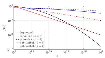
Figure 1: Comparison of the tails of log-normal (black), power-law (red) and sub-Weibull (blue) probability density functions $f(x)$ (log-scales on both axis).

Remark 3 (Bandwidths and estimation of spectral densities).

The results in Propositions 1 and 2 require uniform consistency of the estimated spectral density over all frequencies. For this reason, we have stronger than usual asymptotic constraints on the bandwidths. These could be relaxed if we made stronger assumptions on the shocks. First, notice that in our setting the level shocks are just uncorrelated (see Assumptions (L1i) and (L1iii)), and are by no means independent. However, if we are willing to assume the existence, for level shocks, of moments of all orders, then we could apply Theorem 7.7.4 in Brillinger, (2001), which would allow us to replace $B_{T}$ with $B_{T}^{\epsilon}\sqrt{B_{T}}$ for any $\epsilon>0$ in the definition of $\rho_{nT}$ in Proposition 1. Second, we could, in principle, allow for independent shocks on log-volatilities (e.g. assuming Gaussianity, see Remark 1) and therefore make use of Theorem 4 and Section 4.2 in Wu and Zaffaroni, (2018), which would allow us to replace $M_{T}$ with $\sqrt{M_{T}\log M_{T}}$ in the definition of $\tau_{nT}$ in Proposition 2.

4 Conditional prediction intervals

Before describing our prediction intervals, let us summarise here the main notation developed in the previous sections. Given an observed dataset of size $n\times T$, we have, for the levels,

$$Y_{it} =X_{it}+Z_{it}+\mathrm{E}[Y_{it}],$$ (4.1)

$$X_{it} =\mathbf{b}_{i0}^{\prime}\mathbf{u}_{t}+\sum_{k=1}^{\infty}\mathbf{b}_{ik}^{\prime}\mathbf{u}_{t-k}:=e_{it}+X_{it|t-1},\quad Z_{it}=d_{i0}v_{it}+\sum_{k=1}^{\infty}d_{ik}v_{it-k}:=v_{it}+Z_{it|t-1},$$

$$s_{it} :=e_{it}+v_{it},\ \ i=1,\ldots,n,\ t=1,\ldots,T$$

where $d_{i0}=1$ because of (2.4) and, for the log-volatilities,

$$h_{it} :=\log s_{it}^{2}=\chi_{it}+\xi_{it}+\mathrm{E}[h_{it}],$$ (4.2)

$$\chi_{it} =\mathbf{f}_{i0}^{\prime}\bm{\varepsilon}_{t}+\sum_{k=1}^{\infty}\mathbf{f}_{ik}^{\prime}\bm{\varepsilon}_{t-k}:=\eta_{it}+\chi_{it|t-1},\quad\xi_{it}=g_{i0}\nu_{it}+\sum_{k=1}^{\infty}g_{ik}\nu_{it-k}:=\nu_{it}+\xi_{it|t-1},$$

$$\omega_{it} :=\eta_{it}+\nu_{it},\ \ i=1,\ldots,n,\ t=1,\ldots,T$$

where $g_{i0}=1$ because of (2.13).

The optimal one-step-ahead linear predictors of level $Y_{it}$ and log-volatility $h_{it}$ are thus

$$Y_{it|t-1}:=X_{it|t-1}+Z_{it|t-1}+\mathrm{E}[Y_{it}]\quad\text{and }\quad h_{it|t-1}:=\chi_{it|t-1}+\xi_{it|t-1}+\mathrm{E}[h_{it}],$$ (4.3)

with innovations $s_{it}$ and $\omega_{it}$, respectively. As a consequence, the level innovations are

$$s_{it}=\exp\big{(}{h_{it}}/{2}\big{)}\mbox{sign}(s_{it})=\exp\big{(}{h_{it|t-1}}/{2}\big{)}\exp\big{(}{\omega_{it}}/{2}\big{)}\mbox{sign}(s_{it}).$$

We therefore define a one-step-ahead predictor of the volatilities as

$$s_{it|t-1}:=\exp\big{(}{h_{it|t-1}}/2\big{)},$$

with associated “multiplicative innovations”

$$w_{it}:=\exp\big{(}{\omega_{it}}/{2}\big{)}\mbox{sign}(s_{it}).$$

Note, however, that, due to the nonlinear nature of the exponential transformation from $h_{i}$ to $s_{i}$, this multiplicative decomposition of volatilities into a predictor and an “innovation” does not enjoy (in the space of volatilities) the traditional $L^{2}$ optimality properties, which only hold for their logarithms (in the space of log-volatilities). This, however, will not be a concern in the quantile-based construction we now describe, due to the fact that the coverage probabilities of a interquantile interval are invariant under continuous monotone transformations: the quantile of $w_{it}$ .

Denoting by $q(\alpha;w_{i})$ the (unconditional) $\alpha$-quantile of $w_{i}:=\{w_{it}|t=1,\ldots,T\}$, $i=1,\ldots,n$ (which, by stationarity, does not depend on $t$), theoretical lower and upper prediction bounds with confidence level $(1-\alpha)$ and $\alpha\in(0,1)$ are

$$\mathcal{L}_{it|t-1}(\alpha):=Y_{it|t-1}+s_{it|t-1}\,q(\alpha;w_{i})\ \text{ and }\ \mathcal{U}_{it|t-1}(\alpha):=Y_{it|t-1}+s_{it|t-1}\,q(1-\alpha;w_{i}),$$ (4.4)

respectively. Note that $Y_{it|t-1}$ lies above $\mathcal{L}_{it|t-1}(\alpha)$ for $\alpha<{\rm P}[w_{it}\leq 0]$ and lies below $\mathcal{U}_{it|t-1}(\alpha)$ for $\alpha<1-{\rm P}[w_{it}\leq 0]$. Prediction intervals with coverage probability $(1-\alpha)$ can be constructed as

$$\mathcal{I}_{it|t-1}(\alpha):=\big{[}\,\mathcal{L}_{it|t-1}(\alpha^{-}),\,\mathcal{U}_{it|t-1}(\alpha^{+})\;\big{]}$$ (4.5)

with $\alpha^{\pm}<1/2$ and $\alpha^{-}+\alpha^{+}=\alpha$, covering $Y_{it|t-1}$ (see (4.8)) provided that

$$\alpha^{-}<{\rm P}[w_{it}\leq 0]\quad\text{ and }\quad\alpha^{+}<1-{\rm P}[w_{it}\leq 0].$$ (4.6)

Clearly, the lower bound $\mathcal{L}_{it|t-1}(\alpha)$ provides a measure of the Value-at-Risk of level $\alpha$ at time $t$, which we denote as ${\rm VaR}_{it}(\alpha):=-\mathcal{L}_{it|t-1}(\alpha)$ (see Section 12.3.1 in Francq and Zakoian, , 2011 for a review).

The advantage of quantile-based prediction intervals of the form (4.5) over their conditional heteroskedasticity-based competitors stems from the fact that, irrespective of the way $w_{i}$ has been obtained, the conditional $\alpha$-quantiles of $Y_{it}$ (conditional on $Y_{i,t-1},Y_{i,t-2},\ldots$) are of the form (4.4). This quantile-based approach moreover allows for unequal tails ($\alpha^{-}\neq\alpha^{+}$ in (4.6)—hence, distinct attitudes towards losses and gains) and automatically takes into account the typical skewness of financial data distributions.

In practice, the model is estimated from a $n\times T$ observed panel; the empirical counterparts of ${Y}_{i,T+1|T}$ and ${h}_{i,T+1|T}$ for $i=1,\ldots,n$ are

$$\widehat{Y}_{i,T+1|T}=\widehat{X}_{i,T+1|T}+\widehat{Z}_{i,T+1|T}+\frac{1}{T}\sum_{t=1}^{T}Y_{it}=\sum_{k=1}^{\bar{k}_{1}}\widehat{\mathbf{b}}_{ik}^{\prime}\widehat{\mathbf{u}}_{T-k+1}+\sum_{k=1}^{\bar{k}_{2}}\widehat{d}_{ik}\widehat{v}_{i,T-k+1}+\frac{1}{T}\sum_{t=1}^{T}Y_{it}\vspace{-3mm}$$

and

$$\widehat{h}_{i,T+1|T}=\widehat{\chi}_{i,T+1|T}+\widehat{\xi}_{i,T+1|T}+\frac{1}{T}\sum_{t=1}^{T}\widehat{h}_{it}=\sum_{k=1}^{\bar{k}_{1}^{*}}\widehat{\mathbf{f}}_{ik}^{\prime}\widehat{\bm{\varepsilon}}_{T-k+1}+\sum_{k=1}^{\bar{k}_{2}^{*}}\widehat{g}_{ik}\widehat{\nu}_{i,T-k+1}+\frac{1}{T}\sum_{t=1}^{T}\widehat{h}_{it},\vspace{-1mm}$$

and we accordingly define $\widehat{s}_{i,T+1|T}:=\exp\big{(}{\widehat{h}_{i,T+1|T}}/{2}\big{)}$; based on the estimates $\widehat{s}_{it}$ and $\widehat{\omega}_{it}$ of $s_{it}$ and $\omega_{it}$, let $\widehat{w}_{it}:=\exp\big{(}{\widehat{\omega}_{it}}/2\big{)}\text{sign}(\widehat{s}_{it})$.

For any $i$, denote by $\widehat{w}_{i(1)},\ldots,\widehat{w}_{i(T)}$ the order statistic of $\widehat{w}_{i1},\ldots,\widehat{w}_{iT}$; the empirical quantile $w_{i(\lceil T\alpha\rceil)}$ then can be used as an estimator of $q(\alpha;w_{i})$. Empirical versions of the prediction limits and intervals (4.4) and (4.5) are

$$\widehat{\mathcal{L}}_{i,T+1|T}(\alpha):=\widehat{Y}_{i,T+1|T}+\widehat{s}_{i,T+1|T}\,\widehat{w}_{i(\lceil T\alpha\rceil)},\quad\widehat{\mathcal{U}}_{i,T+1|T}(\alpha):=\widehat{Y}_{i,T+1|T}+\widehat{s}_{i,T+1|T}\,\widehat{w}_{i(\lceil T(1-\alpha)\rceil)}$$

and

$$\widehat{\mathcal{I}}_{i,T+1|T}(\alpha):=\big{[}\widehat{\mathcal{L}}_{i,T+1|T}(\alpha^{-}),\widehat{\mathcal{U}}_{i,T+1|T}(\alpha^{+})\big{]}$$ (4.7)

with $\alpha^{\pm}<1/2$ and $\alpha^{-}+\alpha^{+}=\alpha\in(0,1)$. A schematic description of this procedure is given in Algorithm 3.

If the $w_{it}$’s were i.i.d.  instead of weak white noise, the convergence (for given $\alpha^{-}$ and $\alpha^{+}$, without rates) of (4.7) to (4.5) would follow from the fact that, as a consequence of the consistent estimation of the GDFMs for levels and volatilities, for any $n_{0}$ and $T_{0}$, $\max_{1\leq i\leq n_{0}}\max_{1\leq t\leq T_{0}}|\widehat{w}_{it}-w_{it}|$ converges to zero as $n$ and $T$ tend to infinity.

Then, the difference between the empirical quantile of order $\alpha$ computed from $\{\widehat{w}_{1t},\ldots,\widehat{w}_{iT_{0}}\}$ and the empirical quantile of order $\alpha$ computed from the unobservable $\{w_{i1},\ldots,w_{iT_{0}}\}$ is $o_{\rm P}(1)$ for given $1\leq i\leq n_{0}$ as $n$ and $T$ tend to infinity. Now, for given $i$, were the $w_{it}$’s i.i.d., the empirical $\alpha$-quantile computed from $\{w_{i1},\ldots,w_{iT_{0}}\}$ is, for $T_{0}$ large enough, arbitrarily close to its theoretical counterpart $q(\alpha;w_{i})$ with probability arbitrarily close to one. The same conclusion extends to the present case where the $w_{it}$’s are stationary and uncorrelated provided that they satisfy some additional mild ergodicity or mixing assumption. The literature on Glivenko-Cantelli and quantile consistency under ergodicity and mixing is abundant, and we will not proceed with imposing any specific mixing conditions here which anyway hardly can be checked from the data. The reader may like to refer to Theorem 3.1 in Francq and Zakoian, (2019) for details.

Once prediction regions have been constructed, it is important to evaluate their actual coverage performance. For this, it is useful to define the conditional coverage indicators—namely, for prediction intervals $\widehat{\mathcal{I}}_{i,T+1|T}(\alpha)$,

$$\widehat{\mathcal{H}}_{i,T+1|T}(\alpha):=\mathbb{I}\big{(}Y_{i,T+1}\in\widehat{\mathcal{I}}_{i,T+1|T}(\alpha)\big{)}.$$ (4.8)

For a given $i$, we say that $\widehat{\mathcal{I}}_{i,T+1|T}(\alpha)$ provides the correct coverage if

$$\mathrm{P}(Y_{i,T+1}\in\widehat{\mathcal{I}}_{i,T+1|T}(\alpha)|Y_{i,T},\ldots,Y_{i1})=\mathrm{E}[\widehat{\mathcal{H}}_{i,T+1|T}(\alpha)|Y_{i,T},\ldots,Y_{i1}]=(1-\alpha),$$

which is equivalent (see e.g. Lemma 1 in Christoffersen, , 1998) to the hypothesis that

$$\widehat{\mathcal{H}}_{i,T+1|T}(\alpha)\stackrel{{\scriptstyle iid}}{{\sim}}\mbox{Bernoulli}(1-\alpha).$$ (4.9)

That hypothesis can be tested against alternatives of insufficient coverage probability values, against non-sharp prediction limits, or against alternatives of serial dependence. We refer to Section 6.3 for details and implementation.

Input: data in levels $\mathbf{Y}$, $\alpha^{-}\in[0,1/2]$ and $\alpha^{+}\in[0,1/2]$ such that the confidence level is $\alpha=\alpha^{+}+\alpha^{-}\in(0,1)$

from Algorithm 1: common level shocks $\widehat{\mathbf{u}}$ of size $q\times T$ and $\widehat{\mathbf{e}}$ of size $n\times T$, idiosyncratic level shocks $\widehat{\mathbf{v}}$ of size $n\times T$, common level impulse responses $\widehat{\mathbf{B}}(L)$ of size $n\times q\times\bar{k}_{1}$, idiosyncratic level impulse responses $\widehat{\mathbf{D}}(L)$ of size $n\times n\times\bar{k}_{2}$

from Algorithm 2: log-volatility proxy $\mathbf{h}$ of size $n\times T$, common log-volatility shocks $\widehat{\bm{\varepsilon}}$ of size $Q\times T$ and $\widehat{\bm{\eta}}$ of size $n\times T$, idiosyncratic log-volatility shocks $\widehat{\bm{\nu}}$ of size $n\times T$, common level impulse responses $\widehat{\mathbf{F}}(L)$ of size $n\times Q\times\bar{k}_{1}^{*}$, idiosyncratic level impulse responses $\widehat{\mathbf{G}}(L)$ of size $n\times n\times\bar{k}_{2}^{*}$

Output: lower bounds of conditional prediction interval $\widehat{\mathcal{L}}_{1,T+1|T}(\alpha^{-}),\ldots,\widehat{\mathcal{L}}_{n,T+1|T}(\alpha^{-})$

upper bounds of conditional prediction interval $\widehat{\mathcal{U}}_{1,T+1|T}(\alpha^{+}),\ldots,\widehat{\mathcal{U}}_{n,T+1|T}(\alpha^{+})$

1

2Compute $\bar{\mathbf{Y}}$ the sample mean of levels $\mathbf{Y}$ 

3Compute the one-step-ahead prediction of common and idiosyncratic components of levels $\widehat{\mathbf{X}}_{T+1|T}=\sum_{k=1}^{\bar{k}_{1}}\widehat{\mathbf{B}}_{k}\widehat{\mathbf{u}}_{T-k+1}$ 

4Compute the one-step-ahead prediction of idiosyncratic component of levels $\widehat{\mathbf{Z}}_{T+1|T}=\sum_{k=1}^{\bar{k}_{2}}\widehat{\mathbf{D}}_{k}\widehat{\mathbf{v}}_{T-k+1}$ 

5Compute the one-step-ahead prediction of levels $\widehat{\mathbf{Y}}_{T+1|T}=\widehat{\mathbf{X}}_{T+1|T}+\widehat{\mathbf{Z}}_{T+1|T}+\bar{\mathbf{Y}}$ such that $\widehat{\mathbf{Y}}_{T+1|T}=(\widehat{Y}_{1,T+1|T}\ldots\widehat{Y}_{n,T+1|T})^{\prime}$ 

6Compute $\bar{\widehat{\mathbf{h}}}$ the sample mean of log-volatilities $\widehat{\mathbf{h}}$ 

7Compute the one-step-ahead prediction of common component of log-volatilities $\widehat{\bm{\chi}}_{T+1|T}=\sum_{k=1}^{\bar{k}_{1}^{*}}\widehat{\mathbf{F}}_{k}\widehat{\bm{\varepsilon}}_{T-k+1}$ 

8Compute the one-step-ahead prediction of idiosyncratic component of log-volatilities $\widehat{\bm{\xi}}_{T+1|T}=\sum_{k=1}^{\bar{k}_{2}^{*}}\widehat{\mathbf{G}}_{k}\widehat{\bm{\nu}}_{T-k+1}$ 

9Compute the one-step-ahead prediction of log-volatilities $\widehat{\mathbf{h}}_{T+1|T}=\widehat{\bm{\chi}}_{T+1|T}+\widehat{\bm{\xi}}_{T+1|T}+\bar{\widehat{\mathbf{h}}}$ 

10Compute the one-step-ahead prediction of volatilities $\widehat{\mathbf{s}}_{T+1|T}=\exp(\widehat{\mathbf{h}}_{T+1|T}/2)$ such that $\widehat{\mathbf{s}}_{T+1|T}=(\widehat{s}_{1,T+1|T}\ldots\widehat{s}_{n,T+1|T})^{\prime}$  

11Compute the log-volatility innovations $\widehat{\bm{\omega}}_{t}=\widehat{\bm{\eta}}_{t}+\widehat{\bm{\nu}}_{t}$ for $t=1,\ldots,T$ 

12Compute the volatility proxy $\widehat{\mathbf{s}}_{t}=\exp(\mathbf{h}_{t}/2)$ or equivalently $\widehat{\mathbf{s}}_{t}=\widehat{\mathbf{e}}_{t}+\widehat{\mathbf{v}}_{t}$ for $t=1,\ldots,T$ 

13Compute the volatility innovations $\widehat{\mathbf{w}}_{t}=\exp(\widehat{\bm{\omega}}_{t}/2)\mbox{sign}(\widehat{\mathbf{s}}_{t})$ such that $\widehat{\mathbf{w}}_{t}=(\widehat{w}_{1t}\ldots\widehat{w}_{nt})^{\prime}$ for $t=1,\ldots,T$  

14for $i\leftarrow 1$ to $n$ do

15      Compute the order statistics $w_{i(\lceil T\alpha^{-}\rceil)}$ and $w_{i(\lceil T(1-\alpha^{+})\rceil)}$ of $w_{i}$ 

16      Compute the lower bound $\widehat{\mathcal{L}}_{i,T+1|T}(\alpha^{-})=\widehat{Y}_{i,T+1|T}+\widehat{s}_{i,T+1|T}\,\widehat{w}_{i(\lceil T\alpha^{-}\rceil)}$ 

17      Compute the upper bound $\widehat{\mathcal{U}}_{i,T+1|T}(\alpha^{+})=\widehat{Y}_{i,T+1|T}+\widehat{s}_{i,T+1|T}\,\widehat{w}_{i(\lceil T(1-\alpha^{+})\rceil)}$ 

18

Algorithm 3 Estimation of conditional prediction intervals

5 Simulation study

5.1 Setup

To study the performance of our estimator on finite samples, we simulate data ($\mathcal{M}$ replications) according to the model described in (4.1)-(4.2).

For each Monte Carlo replication $m=1,\ldots,\mathcal{M}$ and for given values of $n,T,q$, and $Q$, we first simulate a multiplicative factor model for the volatilities which in turn implies a factor structure also for the levels. The common component of the log-volatilities is generated as

$$\bm{\chi}_{nt,m}:=(\mathbf{M}_{n,m}(L))^{-1}\mathbf{R}_{n,m}\bm{\varepsilon}_{t,m},\quad t=1,\ldots,T,$$

where $\bm{\varepsilon}_{t,m}\stackrel{{\scriptstyle iid}}{{\sim}}N(\mathbf{0}_{Q},\mathbf{I}_{Q})$, $\mathbf{R}_{n,m}$ is $n\times Q$ with entries $[\mathbf{R}_{n,m}]_{ij}\stackrel{{\scriptstyle iid}}{{\sim}}N(0,1)$ and rescaled such that $\mathbf{R}_{n,m}^{\prime}\mathbf{R}_{n,m}=n$,and $\mathbf{M}_{n,m}(L)=\mathbf{I}_{n}-\sum_{k=1}^{3}\mathbf{M}_{kn,m}L^{k}$ where the coefficients $\mathbf{M}_{kn,m}$ are diagonal $n\times n$ matrices with entries $[\mathbf{M}_{kn,m}]_{ij}\stackrel{{\scriptstyle iid}}{{\sim}}N(0,1)$ and rescaled in such a way that $\det(\mathbf{M}_{n,m}(z))\neq 0$ for $|z|\leq 1$. Then, we generate the process

$$\bm{\xi}_{nt,m}^{*}:=(\mathbf{P}_{n,m}^{*}(L))^{-1}\bm{\nu}_{nt,m}^{*},\quad t=1,\ldots,T,$$

where $\bm{\nu}_{nt,m}^{*}\stackrel{{\scriptstyle iid}}{{\sim}}N(\mathbf{0}_{n},\bm{\Sigma}_{n,m})$, with $\bm{\Sigma}_{n,m}$ a Toeplitz matrix with entries $[\bm{\Sigma}_{n,m}]_{ij}:=0.5^{|i-j|}$, if $|i-j|\leq 2$ and zero otherwise, and $\mathbf{P}_{n,m}^{*}(L)$ generated in the same way as $\mathbf{M}_{n,m}(L)$. Denoting by $\xi^{*}_{it,m}$ the $i$th element of $\bm{\xi}^{*}_{it,m}$, we rescale it into $\xi^{**}_{it,m}:=\xi^{*}_{it,m}[\text{\rm Var}(\chi_{it,m})/\{2\text{\rm Var}(\xi^{*}_{it,m})\}]^{1/2}$ so that the signal-to-noise ratio is 2.

Define

$$e_{it,m}^{*} :=\exp(\chi_{it,m}/2)\ \pi_{it,m},\;\mbox{ and }\;v_{it,m}^{*}:=\exp(\chi_{it,m}/2)\ \exp(\xi^{**}_{it,m}/2)\pi_{it,m},\quad t=1,\ldots,T,\ i=1,\ldots,n,$$

where $\pi_{it,m}=\pm 1$ with equal probabilities 0.5 and $\chi_{it,m}$ is the $i$th element of $\bm{\chi}_{t,m}$. The volatility and log-volatility proxies then are

$$s_{it,m}^{2} :=(e_{it,m}^{*}+v_{it,m}^{*})^{2}=\exp(\chi_{it,m})\left[1+\exp(\xi^{**}_{it,m})+2\exp(\xi^{**}_{it,m}/2)\right],$$

$$h_{it,m} :=\log(s_{it,m}^{2})=\chi_{it,m}+\log\left[1+\exp(\xi^{**}_{it,m})+2\exp(\xi^{**}_{it,m}/2)\right],\;t=1,\ldots,T,\ i=1,\ldots,n,$$

from which we see that, since each $\chi_{i,m}$ is driven by the $Q$-dimensional vector of shocks $\bm{\varepsilon}_{m}$, it has the role of common log-volatility, while the $n$ shocks $\bm{\nu}^{*}_{n,m}$ have only an idiosyncratic role.

Letting $\mathbf{V}$ be the $q$ normalized eigenvectors corresponding to the $q$ largest eigenvalues of the sample covariance of the vector $\mathbf{e}_{nt,m}^{*}:=(e_{1t,m}^{*}\ldots e_{nt,m}^{*})^{\prime}$, we build the level shocks as

$$\mathbf{e}_{nt,m} :=\mathbf{V}\mathbf{V}^{\prime}\mathbf{e}^{*}_{nt,m},\;\mbox{ and }\;\mathbf{v}_{nt,m}:=\mathbf{V}_{\perp}\mathbf{V}_{\perp}^{\prime}\mathbf{e}^{*}_{nt,m}+\mathbf{v}_{nt,m}^{*},\quad t=1,\ldots,T,$$

where $\mathbf{V}_{\perp}$ is $n\times(n-q)$ such that $\mathbf{V}_{\perp}^{\prime}\mathbf{V}=\mathbf{0}_{(n-q)\times q}$, and $\mathbf{v}_{nt,m}^{*}:=(v_{1t,m}^{*}\ldots v_{nt,m}^{*})^{\prime}$. Note that, by construction, the elements $e_{it,m}$ and $v_{it,m}$ of the vectors $\mathbf{e}_{nt,m}$ and $\mathbf{v}_{nt,m}$ are such that $(e_{it,m}+v_{it,m})=(e_{it,m}^{*}+v_{it,m}^{*})$: therefore, we can also write $s_{it}^{2}=(e_{it,m}+v_{it,m})^{2}$.

Finally, we generate the vectors of common and idiosyncratic components of the levels as

$$\mathbf{X}_{nt,m} :=(\mathbf{I}_{n}-\mathbf{A}_{n,m}L)^{-1}\mathbf{e}_{nt,m},\;\mbox{ and }\;\mathbf{Z}_{nt,m}:=(\mathbf{I}_{n}-\mathbf{C}_{n,m}L)^{-1}\mathbf{v}_{nt,m},\quad t=1,\ldots,T$$

where $\mathbf{A}_{n,m}$ is a diagonal $n\times n$ matrix with entries $[\mathbf{A}_{n,m}]_{ij}\stackrel{{\scriptstyle iid}}{{\sim}}U[-0.3,0.7]$, and $\mathbf{C}_{n,m}$ is generated in the same way but with entries from a uniform distribution over $[\mathbf{C}_{n,m}]_{ij}\stackrel{{\scriptstyle iid}}{{\sim}}U[-0.5,0.5]$; since these matrices are diagonal, the autoregressive models for $\mathbf{X}_{n,m}$ and $\mathbf{Z}_{n,m}$ are causal. The panel of levels then is generated as $\mathbf{Y}_{nt,m}:=\mathbf{X}_{nt,m}+\mathbf{Z}_{nt,m}$.

In our numerical study, we let $n\in\{100,200\}$, $T\in\{200,500,1000\}$, and either $q=1$ and $Q=1$, $q=3$ and $Q=2$ (as in the empirical application of the next section), or $q=2$ and $Q=3$. For each configuration considered, we simulate and estimate the model $\mathcal{M}=200$ times.

It has to be noticed that the data-generating process we are considering is similar to a stochastic volatility model. To illustrate the properties of the generated data, we report in Table 1 the autocorrelations up to lag 10 of $h_{i,m}$, $s_{i,m}$, $e_{i,m}$, $v_{i,m}$, $X_{i,m}$, $X_{i,m}^{2}$, $Z_{i,m}$, $Z_{i,m}^{2}$, $Y_{i,m}$, and $Y_{i,m}^{2}$, averaged over all $\mathcal{M}$ replications and over all $n$ series, and when $n=200$, $T=1000$. It can be seen that log-volatilities $h_{i,m}$ and volatilities $s_{i,m}$ have high persistence, while, due to the way they are generated, the shocks $e_{i,m}$ and $v_{i,m}$ display no linear serial dependence, i.e. are weak white noises. Turning to the kurtosis of the level shocks reported in the left panel of Table 2, these display heavy tails (especially the common ones) for the case $q=1$ and $Q=1$, while the kurtosis tends to decrease when increasing $Q$, possibly due to the aggregation of shocks in generating the common components of the log-volatility $\chi_{i,m}$. Similar comments apply to the absolute values of skewness reported in the right panel of Table 2: especially in the case $q=1$ and $Q=1$, the common shocks display a high degree of asymmetry. Because of these features of the simulated data the case $q=1$ and $Q=1$ is particularly interesting to study to assess the performance of our estimators when dealing with heavy-tailed and skewed data.

Table 1: Autocorrelations of simulated variables. Average values over all $n$ series and all $\mathcal{M}$ replications for $n=200$, $T=1000$, and $\mathcal{M}=200$. Values outside the $[\pm 1.96/\sqrt{T}]=[\pm 0.0620]$ interval are starred.

$q=1$	lag
$Q=1$	1	2	3	4	5	6
$h_{i,m}$	0.2967*	0.2856*	0.1178*	0.1691*	0.0528	0.1142*
$s_{i,m}$	0.3082*	0.2743*	0.1201*	0.1426*	0.0552	0.0758*
$e_{i,m}$	-0.0378	0.0696*	-0.0565	0.0089	-0.0099	-0.0283
$e^{2}_{i,m}$	0.0326	0.0495	0.0020	0.0035	0.0031	0.0042
$v_{i,m}$	-0.0023	-0.0017	-0.0035	0.0005	-0.0015	-0.0028
$v^{2}_{i,m}$	0.2961*	0.2674*	0.1196*	0.1445*	0.0565	0.0771*
$X_{i,m}$	0.1753*	0.1770*	0.0096	0.0302	-0.0032	-0.0262
$X^{2}_{i,m}$	0.0989*	0.0791*	0.0068	0.0023	0.0016	-0.0037
$Z_{i,m}$	0.0020	0.0783*	-0.0033	0.0118	-0.0018	-0.0002
$Z^{2}_{i,m}$	0.2877*	0.2260*	0.1054*	0.1200*	0.0522	0.0622*
$Y_{i,m}$	0.1174*	0.1439*	0.0051	0.0219	-0.0031	-0.0172
$Y^{2}_{i,m}$	0.0994*	0.0798*	0.0073	0.0023	0.0018	0.0029
$q=3$	lag
$Q=2$	1	2	3	4	5	6
$h_{i,m}$	0.2654*	0.2826*	0.1183*	0.1611*	0.0508	0.1272*
$s_{i,m}$	0.2757*	0.2607*	0.1237*	0.1305*	0.0511	0.0913*
$e_{i,m}$	-0.0089	-0.0690*	-0.0028	0.0304	-0.0353	-0.0071
$e^{2}_{i,m}$	0.1939*	0.0721*	0.0034	0.0166	0.0077	0.0113
$v_{i,m}$	-0.0010	-0.0011	-0.0030	0.0002	-0.0038	-0.0030
$v^{2}_{i,m}$	0.2635*	0.2515*	0.1212*	0.1283*	0.0503	0.0907*
$X_{i,m}$	0.1977*	0.0592	0.0465	0.0492	-0.0142	0.0002
$X^{2}_{i,m}$	0.2545*	0.0822*	0.0161	0.0222	0.0073	0.0101
$Z_{i,m}$	-0.0172	0.0814*	-0.0052	0.0119	-0.0045	-0.0013
$Z^{2}_{i,m}$	0.2708*	0.2133*	0.1076*	0.1059*	0.0502	0.0764*
$Y_{i,m}$	0.1227*	0.0671*	0.0285	0.0374	-0.0123	-0.0003
$Y^{2}_{i,m}$	0.2166*	0.0909*	0.0237	0.0242	0.0079	0.0009
$q=2$	lag
$Q=3$	1	2	3	4	5	6
$h_{i,m}$	0.2730*	0.2692*	0.1254*	0.1717*	0.0494	0.1293*
$s_{i,m}$	0.2375*	0.2348*	0.1036*	0.1481*	0.0238	0.0885*
$e_{i,m}$	-0.0221	0.0127	-0.0204	-0.0001	-0.0071	-0.0067
$e^{2}_{i,m}$	0.0025	0.0640*	0.0222	0.0616	0.0001	0.0134
$v_{i,m}$	-0.0026	-0.0002	0.0000	0.0026	-0.0011	-0.0035
$v^{2}_{i,m}$	0.2330*	0.2313*	0.1015*	0.1456*	0.0229	0.0879*
$X_{i,m}$	0.1835*	0.1254*	0.0364	0.0277	0.0079	0.0008
$X^{2}_{i,m}$	0.1159*	0.1020*	0.0388	0.0377	0.0131	0.0057
$Z_{i,m}$	0.0317	0.0872*	0.0032	0.0156	-0.0008	-0.0007
$Z^{2}_{i,m}$	0.2509*	0.1918*	0.0969*	0.1227*	0.0293	0.0711*
$Y_{i,m}$	0.1313*	0.1121*	0.0253	0.0220	0.0040	0.0012
$Y^{2}_{i,m}$	0.1047*	0.0869*	0.0426	0.0425	0.0043	0.0133

Table 2: Kurtosis and absolute value of skewness of simulated common level shocks $e_{i,m}$ and idiosyncratic level shocks $v_{i,m}$. Maximum and average values over all $n$ series and all $\mathcal{M}$ replications for $n=200$, $T=1000$, and $\mathcal{M}=200$.

	kurtosis						skewness
	$q=1$, $Q=1$		$q=3$, $Q=2$		$q=2$, $Q=3$		$q=1$, $Q=1$		$q=3$, $Q=2$		$q=2$, $Q=3$
	max.	aver.	max.	aver.	max.	aver.	max.	aver.	max.	aver.	max.	aver.
$e_{i,m}$	161.40	83.53	67.60	10.94	31.86	5.60	7.88	0.28	4.08	0.03	2.53	0.02
$v_{i,m}$	15.03	3.02	12.68	3.02	9.36	3.01	1.14	0.01	1.07	0.01	0.85	0.01

Furthermore, notice that $\mathbf{e}_{n,m}$, by construction, is a singular vector (as it should be) and has the role of a common level innovation. Moreover, the elements of $\mathbf{v}_{n,m}$, in general, are cross-sectionally dependent. As a consequence, both $\mathbf{Y}_{n,m}$ and $\mathbf{h}_{n,m}$ have an approximate dynamic factor structure. In Figure 2 we show scree-plots with the ten largest eigenvalues of the zero-frequency sample spectral density matrices of $\mathbf{Y}_{n,m}$ (blue crosses), and $\mathbf{h}_{n,m}$ (red circles), normalized by the largest zero-frequency eigenvalue, averaged over all $\mathcal{M}$ realisations, when $n=200$, $T=1000$, $q=3$, and $Q=2$.

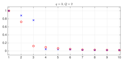
Figure 2: Normalized eigenvalues of the zero-frequency spectral densities of simulated data for $n=200$ and $T=1000$. Blue crosses: levels, $\mathbf{Y}_{n,m}$; red circles: log-volatilities, $\mathbf{h}_{n,m}$.

5.2 Results

For each replication, we estimate the model as described in Section 3. The capping constants $\kappa_{T}$ and the bandwidths $B_{T}$ and $M_{T}$ involved in the estimation of the spectral density are chosen as in the empirical analysis of the next section. Specifically, we let $\kappa_{T}\in\{0,0.2,0.4\}$, while the bandwidths values are $B_{T}=2$ and $M_{T}=10$ for $T=200$, $B_{T}=2$ and $M_{T}=15$ for $T=500$, $B_{T}=2$ and $M_{T}=20$ for $T=1000$ (see Appendix D for results based on other values). Once we obtain estimated common components $\widehat{X}_{i,m}$ for the levels and $\widehat{\chi}_{i,m}$ for the log-volatilities, we compute the global error measures

$$MSE^{X}=\frac{1}{\mathcal{M}nT}\sum_{m=1}^{\mathcal{M}}{\sum_{i=1}^{n}\sum_{t=1}^{T}({X}_{it,m}-\widehat{X}_{it,m})^{2}},\quad MSE^{\chi}=\frac{1}{\mathcal{M}nT}\sum_{m=1}^{\mathcal{M}}\sum_{i=1}^{n}\sum_{t=1}^{T}({\chi}_{it,m}-\widehat{\chi}_{it,m})^{2},$$

$$MAD^{X}=\frac{1}{\mathcal{M}nT}\sum_{m=1}^{\mathcal{M}}{\sum_{i=1}^{n}\sum_{t=1}^{T}|{X}_{it,m}-\widehat{X}_{it,m}|},\quad MAD^{\chi}=\frac{1}{\mathcal{M}nT}\sum_{m=1}^{\mathcal{M}}\sum_{i=1}^{n}\sum_{t=1}^{T}|{\chi}_{it,m}-\widehat{\chi}_{it,m}|$$

and the maximal errors over all realizations:

$$MAX^{X}={\max_{i=1,\ldots,n}\max_{t=1,\ldots,T}\max_{m=1,\ldots,\mathcal{M}}|{X}_{it,m}-\widehat{X}_{it,m}|},$$

$$MAX^{\chi}={\max_{i=1,\ldots,n}\max_{t=1,\ldots,T}\max_{m=1,\ldots,\mathcal{M}}|{\chi}_{it,m}-\widehat{\chi}_{it,m}|}.$$

Notice that the error in the estimation of the common component $X_{i,m}$ of the levels (first step of the estimation procedure) has already been studied in Forni et al., (2017) and Forni et al., (2018). We therefore consider it as the benchmark error with respect to which the performance of the second estimation step, which is the novelty of this paper, is to be compared. Results are provided in Table 3. We note that MSE and MAD in the second step tend to be about 1.5 times higher than in the first step, which is not unexpected as first- and second- step errors typically cumulate in a two-stage procedure. However, when turning to MAX, this is no longer the case, since levels in our data-generating process display heavier tails than log-volatilities—in line with the typical behavior of daily stock returns and their volatilities. Increasing $n$ and $T$ improves the performance of all estimators; the role of $n$, in that respect, seems to be the main one—a manifestation of the “blessing of dimensionality". On the other hand increasing $Q$ the number of common log-volatility shocks, tends to make estimation of the second step harder, but still results are in line with the case $Q=1$. Capping has an effect in controlling the maximum error but does not affect the MSE and MAD results much. To illustrate the good performances of our method, in Figure 3 we show, for one replication, the estimated (in red) and simulated (in blue) common components of levels, and of volatilities, respectively, for $n=200$, $T=1000$, $q=1$, and $Q=1$ (which is the case exhibiting the heaviest tails), setting $\kappa_{T}=0.2$. The choice of bandwidths adopted seems to work quite well, and, comparing to alternative choices considered in Appendix D, it can be shown that $M_{T}$ must be large enough to capture the persistence in log-volatilities, while lower values of $B_{T}$ are enough for levels and do not affect much the second step of estimation.

Table 3: Simulation results. MSEs and MADs for common components. Bandwidths are $B_{T}=2$ and $M_{T}=10$ for $T=200$; $B_{T}=2$ and $M_{T}=15$ for $T=500$; $B_{T}=2$ and $M_{T}=20$ for $T=1000$.

$q=1$, $Q=1$
		$T=200$		$T=500$		$T=1000$
		$n=100$	$n=200$	$n=100$	$n=200$	$n=100$	$n=200$
$MSE^{X}$		0.215	0.219	0.168	0.164	0.125	0.154
$MSE^{\chi}$	$\kappa_{T}=0$	0.368	0.321	0.302	0.247	0.251	0.241
$MSE^{\chi}$	$\kappa_{T}=0.2$	0.369	0.324	0.276	0.247	0.240	0.230
$MSE^{\chi}$	$\kappa_{T}=0.4$	0.377	0.334	0.279	0.238	0.238	0.230
$MAD^{X}$		0.278	0.245	0.255	0.226	0.234	0.228
$MAD^{\chi}$	$\kappa_{T}=0$	0.442	0.401	0.394	0.346	0.360	0.342
$MAD^{\chi}$	$\kappa_{T}=0.2$	0.436	0.395	0.367	0.346	0.344	0.323
$MAD^{\chi}$	$\kappa_{T}=0.4$	0.437	0.397	0.364	0.324	0.337	0.317
$MAX^{X}$		10.797	13.560	17.113	16.352	14.405	19.757
$MAX^{\chi}$	$\kappa_{T}=0$	6.587	6.709	8.996	6.270	7.462	7.912
$MAX^{\chi}$	$\kappa_{T}=0.2$	8.259	7.247	7.967	6.270	9.328	8.431
$MAX^{\chi}$	$\kappa_{T}=0.4$	8.987	8.402	8.295	10.223	9.821	8.960
$q=3$, $Q=2$
		$T=200$		$T=500$		$T=1000$
		$n=100$	$n=200$	$n=100$	$n=200$	$n=100$	$n=200$
$MSE^{X}$		0.143	0.155	0.101	0.112	0.086	0.085
$MSE^{\chi}$	$\kappa_{T}=0$	0.291	0.284	0.237	0.216	0.209	0.185
$MSE^{\chi}$	$\kappa_{T}=0.2$	0.262	0.261	0.197	0.199	0.179	0.163
$MSE^{\chi}$	$\kappa_{T}=0.4$	0.250	0.252	0.182	0.176	0.162	0.141
$MAD^{X}$		0.265	0.261	0.227	0.228	0.210	0.205
$MAD^{\chi}$	$\kappa_{T}=0$	0.412	0.402	0.370	0.348	0.346	0.322
$MAD^{\chi}$	$\kappa_{T}=0.2$	0.389	0.381	0.336	0.327	0.317	0.299
$MAD^{\chi}$	$\kappa_{T}=0.4$	0.378	0.372	0.321	0.307	0.300	0.275
$MAX^{X}$		6.634	8.693	9.682	12.606	10.943	19.277
$MAX^{\chi}$	$\kappa_{T}=0$	5.532	5.624	5.128	6.725	4.488	5.209
$MAX^{\chi}$	$\kappa_{T}=0.2$	5.688	5.800	5.561	6.204	4.813	4.675
$MAX^{\chi}$	$\kappa_{T}=0.4$	5.713	6.180	5.630	7.317	4.978	5.235
$q=2$, $Q=3$
		$T=200$		$T=500$		$T=1000$
		$n=100$	$n=200$	$n=100$	$n=200$	$n=100$	$n=200$
$MSE^{X}$		0.151	0.161	0.112	0.129	0.082	0.085
$MSE^{\chi}$	$\kappa_{T}=0$	0.356	0.323	0.290	0.277	0.247	0.224
$MSE^{\chi}$	$\kappa_{T}=0.2$	0.324	0.299	0.259	0.247	0.210	0.190
$MSE^{\chi}$	$\kappa_{T}=0.4$	0.311	0.287	0.248	0.231	0.193	0.173
$MAD^{X}$		0.279	0.271	0.241	0.248	0.212	0.213
$MAD^{\chi}$	$\kappa_{T}=0$	0.461	0.434	0.414	0.398	0.382	0.360
$MAD^{\chi}$	$\kappa_{T}=0.2$	0.437	0.415	0.387	0.372	0.350	0.327
$MAD^{\chi}$	$\kappa_{T}=0.4$	0.426	0.404	0.376	0.356	0.334	0.311
$MAX^{X}$		5.395	9.180	5.900	8.936	6.210	11.411
$MAX^{\chi}$	$\kappa_{T}=0$	4.833	5.066	5.009	5.654	5.111	5.571
$MAX^{\chi}$	$\kappa_{T}=0.2$	4.988	5.325	5.269	5.998	5.355	5.654
$MAX^{\chi}$	$\kappa_{T}=0.4$	5.058	5.748	5.660	6.208	5.599	5.413

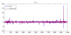
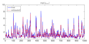
Figure 3: Simulation results. True (blue) and estimated (red) common components of levels, $\widehat{X}_{it,m}$, and of volatilties, $\exp(\widehat{\chi}_{it,m})$, when $n=200$, $T=1000$, $q=1$, $Q=1$, and $\kappa_{T}=0.2$. One series and one realisation.

Finally, for $T=1000$, we estimated the model using the first 900 observations, then ran a recursive pseudo-out-of-sample forecasting exercise constructing one-step-ahead prediction intervals for the remaining $100$ observations (from $901$ to $1000$), as described in Section 4. The $\alpha/2$-upper and $\alpha/2$-lower bounds $\widehat{\mathcal{U}}_{i,\tau+1|\tau,m}(\alpha/2)$ and $\widehat{\mathcal{L}}_{i,\tau+1|\tau,m}(\alpha/2)$ of prediction intervals with coverage probability $(1-\alpha)$ are then computed for each series and replication and each out-of-sample observation. From the latter, we compute the observed coverage frequencies across all series and replications

$$C(\alpha):=\frac{1}{\mathcal{M}n100}\sum_{m=1}^{\mathcal{M}}\sum_{i=1}^{n}\sum_{\tau=900}^{999}\mathbb{I}\Big{(}\widehat{\mathcal{L}}_{i,\tau+1|\tau,m}(\alpha/2)\leq Y_{i,\tau+1,m}\!\leq\widehat{\mathcal{U}}_{i,\tau+1|\tau,m}(\alpha/2)\Big{)}$$

and the proportions of coverage violations in the upper and lower tails,

$$V_{+}(\alpha/2):=\frac{1}{\mathcal{M}n100}\sum_{m=1}^{\mathcal{M}}\sum_{i=1}^{n}\sum_{\tau=900}^{999}\mathbb{I}\Big{(}Y_{i,\tau+1,m}\!>\widehat{\mathcal{U}}_{i,\tau+1|\tau,m}(\alpha/2)\Big{)},$$

and

$$V_{-}(\alpha/2):=\frac{1}{\mathcal{M}n100}\sum_{m=1}^{\mathcal{M}}\sum_{i=1}^{n}\sum_{\tau=900}^{999}\mathbb{I}\Big{(}Y_{i,\tau+1,m}\!<\widehat{\mathcal{L}}_{i,\tau+1|\tau,m}(\alpha/2)\Big{)},$$

respectively. Results are shown in Table 4. Overall performances look reasonably good—the larger $n$ and $T$, the better. We note that capping has a clear effect on the empirical coverage; too much capping seems to affect mostly the cases in which $\alpha=0.32$ and $0.2$. No capping at all works quite well in practice, despite the fact that theoretical results require $\kappa_{T}>0$. Moreover, the same comments apply to empirical coverage as for the choice of bandwidths, with the additional finding that higher values of $B_{T}$ yield more reliable prediction performances (see Appendix D).

Table 4: Simulation results. Empirical coverage and frequencies of prediction bounds violations, averaged over all $n$ series and all $\mathcal{M}$ replications, for $T=1000$ and $\mathcal{M}=200$. Bandwidths values: $B_{T}=2$ and $M_{T}=10$ for $T=200$; $B_{T}=2$ and $M_{T}=15$ for $T=500$; $B_{T}=2$ and $M_{T}=20$ for $T=1000$.

$q=1$, $Q=1$
		$n=100$					$n=200$
		$\alpha$					$\alpha$
		0.32	0.2	0.1	0.05	0.01	0.32	0.2	0.1	0.05	0.01
$C(\alpha)$	$\kappa_{T}=0$	0.6409	0.7637	0.8667	0.9312	0.9869	0.6765	0.7992	0.9082	0.9573	0.9926
$V_{+}(\alpha/2)$		0.1810	0.1195	0.0674	0.0342	0.0057	0.1635	0.1026	0.0470	0.0221	0.0040
$V_{-}(\alpha/2)$		0.1781	0.1168	0.0659	0.0346	0.0074	0.1601	0.0983	0.0449	0.0206	0.0035
$C(\alpha)$	$\kappa_{T}=0.2$	0.6691	0.7769	0.8685	0.9197	0.9681	0.7201	0.8285	0.9226	0.9628	0.9934
$V_{+}(\alpha/2)$		0.1636	0.1124	0.0682	0.0403	0.0153	0.1422	0.0876	0.0392	0.0194	0.0034
$V_{-}(\alpha/2)$		0.1673	0.1107	0.0633	0.0400	0.0166	0.1378	0.0840	0.0383	0.0179	0.0033
$C(\alpha)$	$\kappa_{T}=0.4$	0.7072	0.7987	0.8799	0.9238	0.9699	0.7119	0.7957	0.8763	0.9257	0.9703
$V_{+}(\alpha/2)$		0.1453	0.1023	0.0617	0.0384	0.0145	0.1429	0.1007	0.0600	0.0360	0.0150
$V_{-}(\alpha/2)$		0.1475	0.0990	0.0584	0.0378	0.0156	0.1453	0.1037	0.0638	0.0383	0.0147
$q=3$, $Q=2$
		$n=100$					$n=200$
		$\alpha$					$\alpha$
		0.32	0.2	0.1	0.05	0.01	0.32	0.2	0.1	0.05	0.01
$C(\alpha)$	$\kappa_{T}=0$	0.6350	0.7523	0.8543	0.9131	0.9688	0.6718	0.7917	0.8929	0.9457	0.9895
$V_{+}(\alpha/2)$		0.1810	0.1252	0.0749	0.0449	0.0157	0.1619	0.1037	0.0530	0.0277	0.0053
$V_{-}(\alpha/2)$		0.1840	0.1225	0.0708	0.0420	0.0155	0.1664	0.1047	0.0542	0.0266	0.0053
$C(\alpha)$	$\kappa_{T}=0.2$	0.6767	0.7775	0.8665	0.9206	0.9701	0.7031	0.8081	0.8986	0.9469	0.9916
$V_{+}(\alpha/2)$		0.1601	0.1145	0.0691	0.0422	0.0162	0.1458	0.0935	0.0503	0.0250	0.0039
$V_{-}(\alpha/2)$		0.1632	0.1080	0.0644	0.0372	0.0137	0.1512	0.0985	0.0512	0.0282	0.0046
$C(\alpha)$	$\kappa_{T}=0.4$	0.7129	0.7993	0.8803	0.9267	0.9724	0.7565	0.8447	0.9222	0.9610	0.9923
$V_{+}(\alpha/2)$		0.1445	0.1033	0.0614	0.0384	0.0147	0.1209	0.0780	0.0382	0.0196	0.0043
$V_{-}(\alpha/2)$		0.1426	0.09740	0.0583	0.0349	0.0129	0.1227	0.0774	0.0397	0.0195	0.0035
$q=2$, $Q=3$
		$n=100$					$n=200$
		$\alpha$					$\alpha$
		0.32	0.2	0.1	0.05	0.01	0.32	0.2	0.1	0.05	0.01
$C(\alpha)$	$\kappa_{T}=0$	0.6888	0.8045	0.8981	0.9500	0.9874	0.6391	0.7563	0.8623	0.9215	0.9784
$V_{+}(\alpha/2)$		0.1568	0.0995	0.0527	0.0258	0.0065	0.1786	0.1212	0.0678	0.0387	0.0107
$V_{-}(\alpha/2)$		0.1544	0.0960	0.0492	0.0242	0.0061	0.1824	0.1226	0.0700	0.0399	0.0110
$C(\alpha)$	$\kappa_{T}=0.2$	0.7335	0.8290	0.9105	0.9539	0.9890	0.6770	0.7814	0.8752	0.9277	0.9791
$V_{+}(\alpha/2)$		0.1345	0.0863	0.0459	0.0239	0.0056	0.1602	0.1077	0.0613	0.0355	0.0103
$V_{-}(\alpha/2)$		0.1320	0.0847	0.0436	0.0222	0.0054	0.1629	0.1110	0.0636	0.0368	0.0106
$C(\alpha)$	$\kappa_{T}=0.4$	0.7733	0.8539	0.9213	0.9595	0.9898	0.7167	0.8066	0.8879	0.9352	0.9809
$V_{+}(\alpha/2)$		0.1154	0.0747	0.0408	0.0207	0.0055	0.1395	0.0953	0.0551	0.0326	0.0093
$V_{-}(\alpha/2)$		0.1113	0.0714	0.0379	0.0198	0.0047	0.1439	0.0981	0.0570	0.0322	0.0099

6 Interval prediction for S&P100 returns

In this section, we apply our methodology to a panel of $n=90$ daily returns of stocks from the Standard & Poor’s 100 Index. Data are observed from January 4, 2000 through September 30, 2013, for a total of $T=3456$ observations. We run a pseudo-out-of-sample forecasting exercise by estimating the model using data over the period $t=1,\ldots,\tau$, with $\tau=(T-M),\ldots,(T-1)$ and $M=\leavevmode\nobreak\ \!1948$, corresponding to an evaluation period running from January 3, 2006 through September 27, 2013. For each value of $\tau$, we estimate the $n=90$ one-step-ahead prediction intervals as defined in (4.7). The data cover the following sectors (in parentheses, the number of series in each sector): Consumer Discretionary (11), Consumer Staples (10), Energy (12), Financials (13), Health Care (11), Industrials (14), Information Technology (12), Materials (3), Telecommunications Services (2), Utilities (2) (see Appendix C for the names of individual stocks).

Although we should, in principle, fully re-estimate the whole model at each of the $M$ iterations, some quantities were kept fixed throughout the exercise. In particular, when applied to the full $n\times\leavevmode\nobreak\ \!T$ panel, the Hallin and Liška, (2007) criterion returns $\widehat{q}=3$ common factors for the level panel and $\widehat{Q}=\leavevmode\nobreak\ \!2$ common factors for log-volatility panel: those values are used in all subsequent analyzes. We also choose the bandwidths by minimizing, over a grid of possible bandwidth values, the mean-squared errors

$$\frac{1}{nT}\sum_{i=1}^{n}\sum_{t=1}^{T}(Y_{it}-\widehat{X}_{it|t-1})^{2}\quad\text{and}\quad\frac{1}{nT}\sum_{i=1}^{n}\sum_{t=1}^{T}(\widehat{h}_{it}-\widehat{\chi}_{it|t-1})^{2},$$

respectively, leading to possibly distinct bandwidths for $\widehat{X}_{it|t-1}$ and $\widehat{\chi}_{it|t-1}$. More precisely, we first determine $B_{T}$ and then determine $M_{T}$ using the chosen $B_{T}$ to compute $\widehat{h}_{it}$. As a result we throughout use $B_{T}=2$ and $M_{T}=17$. The VAR orders and the orders of their truncated inverse MA representations needed to compute impulse responses are set as follows: (i) $\text{deg}[\mathbf{A}_{n}(L)]=1$, with inverse MA truncated at lag $\bar{k}_{1}=20$; (ii) $\text{deg}[\mathbf{C}_{n}(L)]=1$, with inverse MA truncated at lag $\bar{k}_{2}=20$; (iii) $\text{deg}[\mathbf{M}_{n}(L)]=5$, with inverse MA truncated at lag $\bar{k}_{1}^{*}=\leavevmode\nobreak\ \!100$; (iv) $\text{deg}[\mathbf{P}_{n}(L)]=1$, with inverse MA truncated at lag $\bar{k}_{2}^{*}=100$. The estimation of the GDFM is based on 10 cross-sectional permutations, as explained at the end of Section 3.1. Finally, regarding the choice of the capping constant $\kappa_{T}$, we choose $\kappa_{T}\in\{0,\,0.1,\,0.25,\,0.5\}$ irrespective of $i$; note that, with reference to Assumption (R), we have $\log^{-1}T=0.12$. Also note that, on the average across the $M$ iterations, 6%, out of the total $n\tau$ observations, are capped when $\kappa_{T}=0.1$, 14% when $\kappa_{T}=\leavevmode\nobreak\ \!0.25$, and 27% when $\kappa_{T}=0.5$.

For any given sample size $\tau$, we compute the quantiles of $\widehat{w}_{i}$ using $(\widehat{w}_{i,\tau-\ell+1},\ldots,\widehat{w}_{i,\tau})$, where weset $\ell\in\{126,252,504,\tau\}$, hence using either the past six months, one year, or two years of available data, or using all available past observations. Denoting by $\widehat{\mathbf{w}}^{(\ell)}_{i}$ the vector of the most recent $\ell$ observations (so that $\widehat{\mathbf{w}}^{(\tau)}_{i}$ coincides with $\widehat{\mathbf{w}}_{i}$), for levels $\alpha\in\{0.32,0.2,0.1,0.05,0.01\}$ and window sizes $\ell$, and for $\tau=(T-M),\ldots,(T-1)$, we obtain the estimates

$$\widehat{\mathcal{U}}_{i,\tau+1|\tau}^{(\ell)}(\alpha):=\widehat{Y}_{i,\tau+1|\tau}+\widehat{s}_{i,\tau+1|\tau}\,\widehat{w}^{(\ell)}_{i(\lceil\ell(1-\alpha)\rceil)}, \quad\quad\quad\widehat{\mathcal{L}}_{i,\tau+1|\tau}^{(\ell)}(\alpha):=\widehat{Y}_{i,\tau+1|\tau}+\widehat{s}_{i,\tau+1|\tau}\,\widehat{w}^{(\ell)}_{i(\lceil\ell\alpha\rceil)},$$

$$\widehat{\mathcal{I}}_{i,\tau+1|\tau}^{(\ell)}(\alpha):=\big{[}\widehat{\mathcal{L}}^{(\ell)}_{i,\tau+1|\tau}(\alpha^{-}),\widehat{\mathcal{U}}^{(\ell)}_{i,\tau+1|\tau}(\alpha^{+})\big{]},\quad\text{ and}\!\!\!\!\!\!\!\!\!\!\!\!\!\!\!\!\!\! \widehat{\mathcal{H}}_{i,\tau+1|\tau}^{(\ell)}(\alpha):=\mathbb{I}\big{(}Y_{i,\tau+1}\in\widehat{\mathcal{I}}_{i,\tau+1|\tau}^{(\ell)}(\alpha)\big{)}.\ \ \ \ \,$$

6.1 Coverage performance: qualitative analysis

For each of the $n=90$ series considered we compute the coverage frequency

$$C_{i}^{(\ell)}(\alpha):=\frac{1}{M}\sum_{\tau=T-M}^{T-1}\widehat{\mathcal{H}}_{i,\tau+1|\tau}^{(\ell)}(\alpha)=\frac{1}{M}\sum_{\tau=T-M}^{T-1}\mathbb{I}\Big{(}\widehat{\mathcal{L}}_{i,\tau+1|\tau}^{(\ell)}(\alpha^{-})\leq Y_{i,\tau+1}\!\leq\widehat{\mathcal{U}}_{i,\tau+1|\tau}^{(\ell)}(\alpha^{+})\Big{)},$$

the proportions

$$V^{(\ell)}_{i,+}(\alpha^{+})\!:=\frac{1}{M}\!\!\sum_{\tau=T-M}^{T-1}\!\!\!\!\mathbb{I}\Big{(}Y_{i,\tau+1}\!>\widehat{\mathcal{U}}_{i,\tau+1|\tau}^{(\ell)}(\alpha^{+})\Big{)}\text{ and }V^{(\ell)}_{i,-}(\alpha^{-})\!:=\frac{1}{M}\!\!\sum_{\tau=T-M}^{T-1}\!\!\!\!\mathbb{I}\Big{(}Y_{i,\tau+1}\!<\widehat{\mathcal{L}}_{i,\tau+1|\tau}^{(\ell)}(\alpha^{-})\Big{)}$$

of coverage violations in the upper and lower tails, and the average interval length

$$L_{i}^{(\ell)}(\alpha):=\frac{1}{M}\sum_{\tau=T-M}^{T-1}\left(\widehat{\mathcal{U}}_{i,\tau+1|\tau}^{(\ell)}(\alpha)-\widehat{\mathcal{L}}_{i,\tau+1|\tau}^{(\ell)}(\alpha)\right).$$

Table 5 reports, for $\alpha^{+}=\alpha^{-}=\alpha/2$ with $\alpha\in\{0.32,0.2,0.1,0.05,0.01\}$ (corresponding to coverage levels 68%, 80%, 90%, 95% and 99%) and $\kappa_{T}\in\{0,0.1,0.25,0.5\}$, the cross-sectional average $C^{(\ell)}(\alpha)$ of the empirical coverage frequencies $C_{i}^{(\ell)}(\alpha)$, the cross-sectional averages $V^{(\ell)}_{+}(\alpha/2)$ and $V^{(\ell)}_{-}(\alpha/2)$ of the proportions of coverage violations $V^{(\ell)}_{i,+}(\alpha^{+})$ and $V^{(\ell)}_{i,-}(\alpha^{-})$, and the cross-sectional average ${L}^{(\ell)}(\alpha)$ of the average interval lengths $L_{i}^{(\ell)}(\alpha)$.

Table 5: Standard & Poor’s 100 Index data ($n=90$ daily returns). Empirical coverage, frequency of prediction bounds violations, and average length of prediction intervals for GDFM, averaged over the cross-section.

	$\kappa_{T}=0$					$\kappa_{T}=0.1$
	$\alpha$					$\alpha$
	0.32	0.2	0.1	0.05	0.01	0.32	0.2	0.1	0.05	0.01
$C^{(126)}(\alpha)$	0.6709	0.7894	0.8887	0.9400	0.9812	0.6874	0.7985	0.8931	0.9416	0.9813
$V^{(126)}_{+}(\alpha/2)$	0.1641	0.1048	0.0552	0.0299	0.0094	0.1559	0.1002	0.0533	0.0291	0.0095
$V^{(126)}_{-}(\alpha/2)$	0.1650	0.1058	0.0561	0.0301	0.0094	0.1566	0.1013	0.0536	0.0292	0.0091
${L}^{(126)}(\alpha)$	3.3934	4.5156	6.1305	7.7681	12.4174	3.4726	4.5726	6.1553	7.7698	12.3130
$C^{(252)}(\alpha)$	0.6708	0.7903	0.8902	0.9415	0.9848	0.6882	0.7999	0.8940	0.9424	0.9846
$V^{(252)}_{+}(\alpha/2)$	0.1647	0.1044	0.0544	0.0289	0.0077	0.1560	0.0998	0.0526	0.0287	0.0078
$V^{(252)}_{-}(\alpha/2)$	0.1644	0.1053	0.0554	0.0296	0.0075	0.1558	0.1003	0.0534	0.0289	0.0076
${L}^{(252)}(\alpha)$	3.3621	4.4794	6.0949	7.7240	12.5008	3.4351	4.5290	6.1078	7.7074	12.3767
$C^{(504)}(\alpha)$	0.6711	0.7895	0.8895	0.9412	0.9846	0.6886	0.7995	0.8929	0.9419	0.9843
$V^{(504)}_{+}(\alpha/2)$	0.1651	0.1057	0.0551	0.0290	0.0078	0.1561	0.1005	0.0536	0.0288	0.0081
$V^{(504)}_{-}(\alpha/2)$	0.1638	0.1047	0.0554	0.0298	0.0076	0.1553	0.1000	0.0535	0.0292	0.0076
${L}^{(504)}(\alpha)$	3.3034	4.4179	6.0266	7.6643	12.1190	3.3786	4.4708	6.0439	7.6539	12.0462
$C^{(\tau)}(\alpha)$	0.7010	0.8142	0.9049	0.9506	0.9881	0.7187	0.8244	0.9096	0.9523	0.9881
$V^{(\tau)}_{+}(\alpha/2)$	0.1516	0.0933	0.0474	0.0247	0.0061	0.1424	0.0879	0.0452	0.0237	0.0062
$V^{(\tau)}_{-}(\alpha/2)$	0.1474	0.0925	0.0477	0.0248	0.0058	0.1389	0.0877	0.0452	0.0239	0.0057
${L}^{(\tau)}(\alpha)$	3.4523	4.6632	6.4305	8.2802	13.3895	3.5562	4.7560	6.5201	8.3747	13.5115
	$\kappa_{T}=0.25$					$\kappa_{T}=0.5$
	$\alpha$					$\alpha$
	0.32	0.2	0.1	0.05	0.01	0.32	0.2	0.1	0.05	0.01
$C^{(126)}(\alpha)$	0.7126	0.8141	0.8997	0.9452	0.9821	0.7552	0.8391	0.9119	0.9507	0.9836
$V^{(126)}_{+}(\alpha/2)$	0.1435	0.0926	0.0500	0.0274	0.0091	0.1222	0.0800	0.0436	0.0243	0.0082
$V^{(126)}_{-}(\alpha/2)$	0.1439	0.0932	0.0504	0.0274	0.0088	0.1226	0.0809	0.0446	0.0251	0.0081
${L}^{(126)}(\alpha)$	3.6203	4.6949	6.2419	7.8371	12.3547	3.9076	4.9426	6.4443	8.0189	12.5330
$C^{(252)}(\alpha)$	0.7138	0.8143	0.9009	0.9452	0.9851	0.7556	0.8398	0.9127	0.9512	0.9866
$V^{(252)}_{+}(\alpha/2)$	0.1433	0.0928	0.0491	0.0271	0.0077	0.1224	0.0798	0.0432	0.0242	0.0069
$V^{(252)}_{-}(\alpha/2)$	0.1428	0.0929	0.0500	0.0277	0.0072	0.1219	0.0804	0.0440	0.0246	0.0065
${L}^{(252)}(\alpha)$	3.5796	4.6500	6.1923	7.7700	12.4405	3.8737	4.9105	6.4108	7.9706	12.7086
$C^{(504)}(\alpha)$	0.7149	0.8150	0.9002	0.9449	0.9846	0.7588	0.8422	0.9132	0.9514	0.9861
$V^{(504)}_{+}(\alpha/2)$	0.1430	0.0927	0.0495	0.0274	0.0080	0.1204	0.0782	0.0426	0.0236	0.0072
$V^{(504)}_{-}(\alpha/2)$	0.1420	0.0923	0.0502	0.0277	0.0074	0.1208	0.0795	0.0442	0.0250	0.0067
${L}^{(504)}(\alpha)$	3.5336	4.6035	6.1513	7.7434	12.1898	3.8584	4.9070	6.4371	8.0357	12.6302
$C^{(\tau)}(\alpha)$	0.7430	0.8387	0.9162	0.9551	0.9886	0.7824	0.8633	0.9283	0.9613	0.9900
$V^{(\tau)}_{+}(\alpha/2)$	0.1301	0.0808	0.0415	0.0221	0.0061	0.1091	0.0680	0.0351	0.0189	0.0053
$V^{(\tau)}_{-}(\alpha/2)$	0.1269	0.0805	0.0422	0.0228	0.0054	0.1085	0.0687	0.0366	0.0198	0.0047
${L}^{(\tau)}(\alpha)$	3.7420	4.9317	6.6982	8.5677	13.7991	4.1045	5.2913	7.0734	8.9901	14.4295

Inspection of the table reveals that $C^{(\ell)}(\alpha)\simeq(1-\alpha)$ and $V_{+}^{(\ell)}(\alpha/2)\simeq V_{-}^{(\ell)}(\alpha/2)\simeq\alpha/2$, which is a qualitative confirmation of the validity of our methodology (see Section 6.3 for more formal validation). Three remarks emerge from these results. First, regarding the sensitivity of our procedure to capping, lower values of $\kappa_{T}$, in general, provide better results when $\alpha$ is higher, while larger values of $\kappa_{T}$ provide better results for lower values of $\alpha$; in all cases, $\kappa_{T}=0.5$ yields a mostly conservative coverage frequency higher than $(1-\alpha)$. In particular, note that the choice of $\kappa_{T}=0$ (no capping at all), although ruled out by Assumption (R), still provides very good results. Second, setting $\ell=\tau$, that is, considering the entire past history to compute quantiles apparently is not the best strategy, and shorter horizons $\ell$ seem preferable. This finding is possibly related to some time variation in the distribution of the innovations of log-volatilities at horizons longer than one year. Third, for any given $\alpha$, shorter intervals are obtained when setting $\ell=252$ or $504$ regardless of the choice of $\kappa_{T}$. Overall, choosing $\kappa_{T}=0.1$ and $\ell=252$ or $504$ works best for $\alpha=0.32$ and $0.2$, while $\kappa_{T}=0.25$ and $\ell=126$ or $252$ works best for $\alpha=0.1,0.05$, and $0.01$.

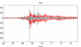
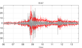
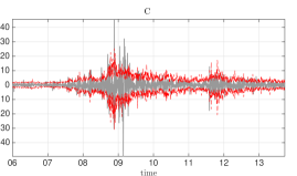
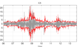
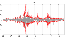
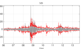
Figure 4: One-step-ahead 90% conditional prediction intervals (in red; $\ell=252$): America International Group (AIG), Bank of America (BAC), Citigroup (C), Goldman Sachs (GS), JPMorgan Chase (JPM), Morgan Stanley (MS).

In Figures 4 and 5, we set $\kappa_{T}=0.25$ and $\ell=252$ and we show (in grey) $Y_{i,\tau+1}$ for some selected individual stocks, together with (in red) the estimated upper and lower bounds of the 90% one-step-ahead prediction interval, i.e. $\widehat{\mathcal{U}}^{(252)}_{i,\tau+1|\tau}(0.05)$ and $\widehat{\mathcal{L}}^{(252)}_{i,\tau+1|\tau}(0.05)$, respectively. Figure 4 shows results for six of the most volatiles stocks in our dataset, all belonging to the financial sector: America International Group (AIG), Bank of America (BAC), Citigroup (C), Goldman Sachs (GS), JPMorgan Chase (JPM), Morgan Stanley (MS). Figure 5 provides the same results for eight relevant non-financial stocks: Apple (AAPL), Microsoft (MSFT), Amazon (AMZN), Wallgreens (WAG), Exxon Mobil (XOM), Johnson & Johnson (JNJ), Boeing (BA), General Electric (GE). Volatilities, in those series, which were the most seriously affected by the great financial crisis, are notoriously hard to predict.

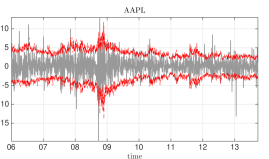
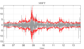
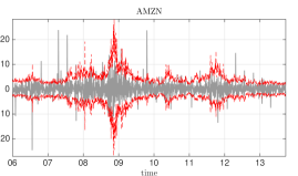
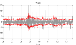
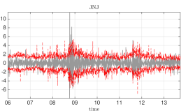
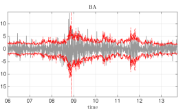
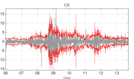
Figure 5: One-step-ahead 90% conditional prediction intervals (in red; $\ell=252$): Apple (AAPL), Microsoft (MSFT), Amazon (AMZN), Wallgreens (WAG), Exxon Mobil (XOM), Johnson & Johnson (JNJ), Boeing (BA), General Electric (GE).

6.2 Coverage: comparison with GARCH

The novelty of our prediction intervals is that they are exploiting the information contained in the available cross-section of $n=90$ stocks. This is in sharp contrast with the usual GARCH approach, which is strongly univariate, and disregards cross-sectional information by analyzing the $n$ series one by one. Moreover, estimating 90 univariate GARCH models requires much more computing time than estimating our model. GARCH nevertheless constitute the more common practice in this context, and serves as a natural benchmark.

We therefore compare our prediction intervals with those obtained by fitting, via quasi-maximum likelihood, univariate GARCH(1,1) models to all series in our panel. Specifically, for each series $i$, we estimate the model

$$Y_{it} =\mathrm{E}[y_{it}]+\sigma_{it}\epsilon_{it},\quad\epsilon_{it}\stackrel{{\scriptstyle iid}}{{\sim}}(0,1),\qquad t=1,\ldots,\tau,$$

$$\sigma_{it}^{2} =\omega_{i}+\gamma_{i}Y_{it-1}^{2}+\beta_{i}\sigma_{it-1}^{2},\quad\omega_{i}>0,\ \gamma_{i},\beta_{i}\geq 0,\ \gamma_{i}+\beta_{i}<1.$$

For given $\tau=(T-M),\ldots,(T-1)$, we obtain estimated parameters $\widehat{\omega}_{i},\widehat{\gamma}_{i}$ and $\widehat{\beta}_{i}$, from which we compute the estimated volatilities $\widehat{\sigma}_{it}^{2}$ and the innovation values $\widehat{\epsilon}_{it}=Y_{it}/\widehat{\sigma}_{it}$, $t=1,\ldots,\tau$. Innovation quantiles are computed from $(\widehat{\epsilon}_{i,\tau-\ell+1},\ldots,\widehat{\epsilon}_{i,\tau})$, where as before we set $\ell\in\{126,\,252,\,504,\,\tau\}$. Then, for any given level $\alpha$ and window size $\ell$, and for $\tau=(T-M),\ldots,(T-1)$, given the one-step-ahead volatility pre- dictor $\widehat{\sigma}_{i,\tau+1|\tau}^{2}=\widehat{\omega}_{i}+\widehat{\gamma}_{i}Y_{i,\tau}^{2}+\widehat{\beta}_{i}\widehat{\sigma}_{i,\tau}^{2}$, we compute the the upper and lower confidence bounds

$$\widehat{\mathcal{U}}_{i,\tau+1|\tau}^{(\ell)\text{\tiny GARCH}}(\alpha):=\bar{Y}_{i}+\widehat{\sigma}_{i,\tau+1|\tau}\,\widehat{\epsilon}^{(\ell)}_{i(\lceil\ell(1-\alpha)\rceil)}\quad\text{and}\quad\widehat{\mathcal{L}}_{i,\tau+1|\tau}^{(\ell)\text{\tiny GARCH}}(\alpha):=\bar{Y}_{i}+\widehat{\sigma}_{i,\tau+1|\tau}\,\widehat{\epsilon}^{(\ell)}_{i(\lceil\ell\alpha\rceil)},$$

yielding the one-step-ahead prediction intervals

$$\widehat{\mathcal{I}}_{i,\tau+1|\tau}^{(\ell)\text{\tiny GARCH}}(\alpha):=\big{[}\widehat{\mathcal{L}}^{(\ell)\text{\tiny GARCH}}_{i,\tau+1|\tau}(\alpha/2),\widehat{\mathcal{U}}^{(\ell)\text{\tiny GARCH}}_{i,\tau+1|\tau}(\alpha/2)\big{]}$$

and the indicators of correct interval prediction $\widehat{\mathcal{H}}_{i,\tau+1|\tau}^{(\ell)\text{\tiny GARCH}}(\alpha):=\mathbb{I}(Y_{i,\tau+1}\in\widehat{\mathcal{I}}_{i,\tau+1|\tau}^{(\ell)\text{\tiny GARCH}}(\alpha))$. Based on these quantities, we then compute, for $\alpha\in\{0.32,\,0.2,\,0.1,\,0.05,\,0.01\}$, the empirical coverage frequency, denoted as $C_{i}^{(\ell)\text{\tiny{GARCH}}}(\alpha)$, the proportions of coverage violations in the upper and lower tail, denoted as $V_{i,+}^{(\ell)\text{\tiny{GARCH}}}(\alpha/2)$ and $V_{i,-}^{(\ell)\text{\tiny{GARCH}}}(\alpha/2)$, respectively, and the average interval length, denoted as ${L}_{i}^{(\ell)\text{\tiny{GARCH}}}(\alpha)$. Averages of these quantities over the $n$ series under study are shown in Table 6. Inspection of this table reveals that the GDFM performances are slightly better than the GARCH ones in terms of coverage frequencies, based on similar interval lengths. This, however, is mainly a descriptive and, due to cross-sectional dependence, somewhat misleading assessment, which ideally should be reinforced into a more formal testing analysis.

Table 6: Standard & Poor’s 100 Index data ($n=90$ daily returns). Empirical coverage, frequency of prediction bounds violations, and average length of prediction intervals for GARCH, averaged over the cross-section.

	$\alpha$
	0.32	0.2	0.1	0.05	0.01
$C^{(126)\text{\tiny{GARCH}}}(\alpha)$	0.6755	0.7947	0.8933	0.9429	0.9834
$V_{+}^{(126)\text{\tiny{GARCH}}}(\alpha/2)$	0.1576	0.0991	0.0507	0.0267	0.0076
$V_{-}^{(126)\text{\tiny{GARCH}}}(\alpha/2)$	0.1669	0.1062	0.0560	0.0304	0.0090
$L^{(126)\text{\tiny{GARCH}}}(\alpha)$	3.4401	4.5562	6.1207	7.7282	12.3986
$C^{(252)\text{\tiny{GARCH}}}(\alpha)$	0.6786	0.7981	0.8968	0.9460	0.9871
$V_{+}^{(252)\text{\tiny{GARCH}}}(\alpha/2)$	0.1567	0.0978	0.0491	0.0255	0.0060
$V_{-}^{(252)\text{\tiny{GARCH}}}(\alpha/2)$	0.1647	0.1041	0.0541	0.0285	0.0069
$L^{(252)\text{\tiny{GARCH}}}(\alpha)$	3.4142	4.5235	6.0755	7.6329	12.2536
$C^{(504)\text{\tiny{GARCH}}}(\alpha)$	0.6807	0.7994	0.8983	0.9479	0.9878
$V_{+}^{(504)\text{\tiny{GARCH}}}(\alpha/2)$	0.1560	0.0975	0.0488	0.0248	0.0056
$V_{-}^{(504)\text{\tiny{GARCH}}}(\alpha/2)$	0.1633	0.1031	0.0529	0.0274	0.0066
$L^{(504)\text{\tiny{GARCH}}}(\alpha)$	3.3822	4.4801	6.0220	7.5581	11.7469
$C^{(\tau)\text{\tiny{GARCH}}}(\alpha)$	0.6920	0.8077	0.9036	0.9510	0.9897
$V_{+}^{(\tau)\text{\tiny{GARCH}}}(\alpha/2)$	0.1520	0.0935	0.0458	0.0228	0.0048
$V_{-}^{(\tau)\text{\tiny{GARCH}}}(\alpha/2)$	0.1560	0.0988	0.0505	0.0262	0.0055
$L^{(\tau)\text{\tiny{GARCH}}}(\alpha)$	3.4139	4.4942	6.0156	7.5369	11.6268

A formal comparison between the GDFM and GARCH(1,1) coverage performances should take into account the fact that the coverage results of the two methods, for given $i$ and $\tau$, are not independent. The situation is quite similar to that of comparing paired proportions, where tests are to be carried out on the basis of the traditional McNemar, (1947) test. For given $\alpha$ and $\ell$, consider, for all $i$, the events (discordant GDFM and GARCH coverage results)

$$\mathcal{A}_{i,\tau+1|\tau}^{(\ell)}(\alpha) :=\left\{Y_{i,\tau+1}\in\widehat{\mathcal{I}}_{i,\tau+1|\tau}^{(\ell)}(\alpha)\cap Y_{i,\tau+1}\notin\widehat{\mathcal{I}}_{i,\tau+1|\tau}^{(\ell)\text{\tiny GARCH}}(\alpha)\right\}$$

$$\mathcal{B}_{i,\tau+1|\tau}^{(\ell)}(\alpha) :=\left\{Y_{i,\tau+1}\notin\widehat{\mathcal{I}}_{i,\tau+1|\tau}^{(\ell)}(\alpha)\cap Y_{i,\tau+1}\in\widehat{\mathcal{I}}_{i,\tau+1|\tau}^{(\ell)\text{\tiny GARCH}}(\alpha)\right\},$$

and define

$$n_{12i}^{(\ell)}(\alpha):=\sum_{\tau=T-M}^{T-1}\mathbb{I}\left(\mathcal{A}_{i,\tau+1|\tau}^{(\ell)}(\alpha)\right)\quad\text{ and }\quad n_{21i}^{(\ell)}(\alpha):=\sum_{\tau=T-M}^{T-1}\mathbb{I}\left(\mathcal{B}_{i,\tau+1|\tau}^{(\ell)}(\alpha)\right).$$

Consider the null hypothesis under which the indicators of a successful interval prediction in both methods are i.i.d. Bernoulli, with identical (but otherwise unspecified) coverage probabilities. The McNemar test of that hypothesis is conditioning on the sum $n_{\text{disc},i}^{(\ell)}(\alpha):=n_{12i}^{(\ell)}(\alpha)+n_{21i}^{(\ell)}(\alpha)$ of discordant coverage results: concordant results indeed carry no information on a difference between coverage probabilities. Conditional on $n_{\text{disc},i}^{(\ell)}(\alpha)$, the null distribution of $n_{12i}^{(\ell)}(\alpha)$ is binomial Bin$(n_{\text{disc},i}^{(\ell)}(\alpha),\,0.5)$. At probability level $\delta$, the test rejects in favour of a better GDFM coverage for “large values” of $n_{12i}^{(\ell)}(\alpha)$, in favour of a better GARCH coverage for “small values” of the same (equivalently, “large values” of $n^{(\ell)}_{21i}$), with critical values the $(1-\delta)$ and $\delta$ binomial quantiles, respectively.

Table 7 reports the McNemar empirical rejection frequencies (over the $n=90$ series)—in favour of a better GDFM coverage in the left-hand panel, in favour of a better GARCH coverage in the right-hand one. We consider the cases in which $\alpha=0.1$ or $0.05$, $\ell=126$ or $252$, $\kappa_{T}=0.25$ (for the GDFM); testing was performed at significance levels $\delta=0.1$, $0.05$, and $0.01$. Irrespective of $\ell$ and $\alpha$, the GDFM approach appears to outperform, quite consistently and significantly, the GARCH one.

Table 7: Standard & Poor’s 100 Index data ($n=90$ daily returns). Proportions of McNemar rejections in favour of a better GDFM coverage (left-hand panel), in favour of a better GARCH coverage (right-hand panel).

	better GDFM coverage			better GARCH coverage
$\alpha=0.1$	$\delta=0.1$	$\delta=0.05$	$\delta=0.01$	$\delta=0.1$	$\delta=0.05$	$\delta=0.01$
$\ell=126$	0.6000	0.5444	0.3667	0.1000	0.0778	0.0667
$\ell=252$	0.5333	0.4556	0.2889	0.1333	0.1222	0.0889
$\alpha=0.05$	$\delta=0.1$	$\delta=0.05$	$\delta=0.01$	$\delta=0.1$	$\delta=0.05$	$\delta=0.01$
$\ell=126$	0.4111	0.2778	0.1556	0.1111	0.0778	0.0556
$\ell=252$	0.2556	0.2000	0.0556	0.1778	0.1222	0.1111

6.3 Coverage: backtesting

As explained in Section 4, a formal assessment of the validity of our approach can be based on the backtesting procedure proposed by Christoffersen, (1998). The idea consists in testing the null hypothesis (4.9) under which the $\widehat{\mathcal{H}}_{i,\tau+1|\tau}(\alpha)$’s (the indicators of a successful interval prediction) are i.i.d. Bernoulli$(1-\alpha)$. Depending on the objectives, several alternatives can be considered. One can be interested (Section 6.3.1) in the validity of interval prediction or the sharpness of the nominal coverage level. Else, one may consider (Section 6.3.2) alternatives of serial dependence. Or, those two issues can be combined (Section 6.3.3) by merging the corresponding alternatives.

Irrespective of the alternative, however, it should be insisted that all those tests—one for each cross-sectional item—are intrinsically univariate. When simultaneously performing several or all of them, one should be extremely cautious with the interpretation of the results. The tables we are providing below are reporting empirical rejection frequencies (over the $n=90$ series). Those $n$ tests, however, are not functionally interrelated (as they would be if the prediction intervals were based on the quantiles of common shocks only); hence, they are not about testing the validity of joint prediction intervals with global asymptotic coverage level $(1-\alpha)$. Neither are they mildly interrelated (as they would be if the prediction intervals were exclusively based on idiosyncratic quantiles), providing joint prediction intervals with global asymptotic coverage level of the order of $(1-\alpha)^{n}$. High rejection frequencies across the $n$ series thus do not imply bad forecasting properties, but can result from complex cross-sectional dependencies. A standard attitude would consist in adopting a Bonferroni or a Šidák correction; for $n=90$, and for a global testing level of $1\%$, this would lead to implementing the $n=90$ individual tests at an overly conservative level $\delta\approx 0.0001=10^{-4}$—a level at which none of the null hypotheses under study is rejected.

All tests below are performed for $\kappa_{T}=0.25$, $\alpha=0.1$ or $0.05$, $\ell=126$ or $252$; testing significance levels are $\delta=0.1$, $0.05$, and $0.01$.

6.3.1 Testing for valid or sharp conditional coverage probabilities

If we are interested in the validity of interval prediction, the relevant testing problems are (one-sided)

$$H_{0i}:\mathrm{E}[\widehat{\mathcal{H}}_{i,\tau+1|\tau}^{(\ell)}(\alpha)]\geq(1-\alpha)\quad\text{ versus }\quad H_{1i}:\mathrm{E}[\widehat{\mathcal{H}}^{(\ell)}_{i,\tau+1|\tau}(\alpha)]<(1-\alpha).$$ (6.1)

If instead we are interested in testing whether $(1-\alpha)$, as a nominal confidence level, is sharp, the testing problems are (still one-sided)

$$H_{0i}:\mathrm{E}[\widehat{\mathcal{H}}_{i,\tau+1|\tau}^{(\ell)}(\alpha)]\leq(1-\alpha)\quad\text{ versus }\quad H_{1i}:\mathrm{E}[\widehat{\mathcal{H}}^{(\ell)}_{i,\tau+1|\tau}(\alpha)]>(1-\alpha).$$ (6.2)

Both testing problems (6.1) and (6.2), admit a level-$\delta$ uniformly most powerful solution, rejecting $H_{0i}$ whenever the test statistic

$$n_{1i}^{(\ell)}(\alpha):=\sum_{\tau=T-M}^{T-1}\widehat{\mathcal{H}}_{i,\tau+1|\tau}^{(\ell)}(\alpha)$$

falls below the binomial Bin$(M,1-\alpha)$ quantile of order $\delta$ when testing (6.1), or above the Bin$(M,1-\alpha)$ quantile of order $(1-\delta)$ when testing (6.2). Since $M$ is large, the same tests are well approximated by rejecting $H_{0i}$ whenever the proportion $n_{1i}^{(\ell)}(\alpha)/M$ of correct coverage is smaller than $(1-\alpha)-z_{\delta}\sqrt{\alpha(1-\alpha)}$ when testing (6.1), or larger than $(1-\alpha)+z_{\delta}\sqrt{\alpha(1-\alpha)}$ when testing (6.2), where $z_{\delta}$ stands for the $(1-\delta)$ standard normal quantile. A two-sided coverage test can also be computed

$$LR_{\text{cover},i}^{(\ell)}(\alpha):=\big{(}n_{1i}^{(\ell)}(\alpha)-M(1-\alpha)\big{)}^{2}/M\alpha(1-\alpha),$$ (6.3)

with asymptotic $\chi^{2}_{(1)}$ null distribution (as $M\to\infty$).

Table 8 reports the empirical rejection frequencies (over $n=90$ series) when testing (6.1) (left-hand panel) and (6.2) (right-hand panel), respectively and using the normal approximation of the binomial. The general comments above apply when interpreting those tables: the only valid global conclusions are those resulting from Bonferroni or Šidák corrections, which do not lead to any rejections.

Table 8: Standard & Poor’s 100 Index data ($n=90$ daily returns). Proportion of rejections when testing for valid nominal coverage (6.1) (left-hand panel) and for sharp nominal coverage (6.2) (middle panel), and when considering the two-sided test (6.3) (right-hand panel)

	valid nominal coverage test			sharp nominal coverage test			two-sided coverage test
$\alpha=0.1$	$\delta=0.1$	$\delta=0.05$	$\delta=0.01$	$\delta=0.1$	$\delta=0.05$	$\delta=0.01$	$\delta=0.1$	$\delta=0.05$	$\delta=0.01$
$\ell=126$	0.1444	0.1222	0.0889	0.2444	0.1444	0.0333	0.2667	0.1889	0.0778
$\ell=252$	0.1556	0.1333	0.0778	0.3111	0.2111	0.0889	0.3444	0.2556	0.1333
$\alpha=0.05$	$\delta=0.1$	$\delta=0.05$	$\delta=0.01$	$\delta=0.1$	$\delta=0.05$	$\delta=0.01$	$\delta=0.1$	$\delta=0.05$	$\delta=0.01$
$\ell=126$	0.2889	0.1889	0.1333	0.0111	0.0000	0.0000	0.1889	0.1556	0.1000
$\ell=252$	0.3000	0.2000	0.1444	0.0556	0.0111	0.0000	0.2111	0.1556	0.1333

6.3.2 Testing against serial dependence

If the alternative of interest is serial dependence among coverage indicators, we propose considering, for each individual stock $i$, alternatives of binary first-order Markov dependence. More precisely, defining the transition probabilities

$$p_{hk,i}(\alpha)=\mathrm{P}\Big{(}\widehat{\mathcal{H}}^{(\ell)}_{i,\tau+1|\tau}(\alpha)=k\,\Big{|}\,\widehat{\mathcal{H}}^{(\ell)}_{i,\tau|\tau-1}(\alpha)=h\Big{)},\quad h,k=1,0,$$

we consider the testing problem (with unspecified unconditional probability $p_{i}(\alpha)$ of correct coverage)

$$H_{0i}:p_{01,i}(\alpha)=p_{11,i}(\alpha)=:p_{i}(\alpha)\;\quad\text{ versus }\quad H_{1i}:p_{01,i}(\alpha)\neq p_{11,i}(\alpha);$$ (6.4)

note that $p_{01,i}(\alpha)=p_{11,i}(\alpha)$ automatically implies $p_{00,i}(\alpha)=p_{10,i}(\alpha)$. Defining

$$n_{11i}^{(\ell)}(\alpha):=\sum_{\tau=T-M+1}^{T-1}\widehat{\mathcal{H}}_{i,\tau+1|\tau}^{(\ell)}(\alpha)\widehat{\mathcal{H}}_{i,\tau|\tau-1}^{(\ell)}(\alpha),\qquad n_{10i}^{(\ell)}(\alpha):=n_{1i}^{(\ell)}(\alpha)-n_{11i}^{(\ell)}(\alpha),$$

$$n_{01i}^{(\ell)}(\alpha):=\sum_{\tau=T-M+1}^{T-1}\widehat{\mathcal{H}}_{i,\tau+1|\tau}^{(\ell)}(\alpha)\big{(}1-\widehat{\mathcal{H}}_{i,\tau|\tau-1}^{(\ell)}(\alpha)\big{)},\qquad n_{00i}^{(\ell)}(\alpha):=n_{0i}^{(\ell)}(\alpha)-n_{01i}^{(\ell)}(\alpha),$$

the statistics

$$\pi_{i}^{(\ell)}(\alpha):=\big{(}{n_{01i}^{(\ell)}(\alpha)+n_{11i}^{(\ell)}(\alpha)}\big{)}/M$$

are estimators of the $p_{i}(\alpha)$’s under the null, while

$${\pi}_{11i}^{(\ell)}(\alpha) :={n_{11i}^{(\ell)}(\alpha)}/{n_{1i}^{(\ell)}(\alpha)},\qquad\qquad\qquad{\pi}_{10i}^{(\ell)}(\alpha):=1-{\pi}_{11i}^{(\ell)}(\alpha),$$

$${\pi}_{01i}^{(\ell)}(\alpha) :=\ {n_{01i}^{(\ell)}(\alpha)}/\big{(}M-{n_{1i}^{(\ell)}(\alpha)}\big{)},\ \ \text{and}\quad{\pi}_{00i}^{(\ell)}(\alpha):=1-{\pi}_{01i}^{(\ell)}(\alpha)$$

are estimating the transition probabilities $p_{hk,i}(\alpha)$ under the alternative. Log-likelihoods under the null and the alternative are

$$L_{0i}(\alpha)= \,(n_{00i}^{(\ell)}(\alpha)+n_{10i}^{(\ell)}(\alpha))\log[1-\pi_{i}^{(\ell)}(\alpha)]+n_{01i}^{(\ell)}(\alpha)+n_{11i}^{(\ell)}(\alpha)\log[\pi_{i}^{(\ell)}(\alpha)],$$

and

$$L_{1i}^{(\ell)}(\alpha)= \,n_{00i}^{(\ell)}(\alpha)\log[1-{\pi}_{01i}^{(\ell)}(\alpha)]+n_{01i}^{(\ell)}(\alpha)\log[{\pi}_{01i}^{(\ell)}(\alpha)]$$

$$\hskip 93.89409pt+n_{10i}^{(\ell)}(\alpha)\log[1-{\pi}_{11i}^{(\ell)}(\alpha)]+n_{11i}^{(\ell)}(\alpha)\log[{\pi}_{11i}^{(\ell)}(\alpha)],$$

respectively. For any given $i$, $\alpha$ and $\ell$, thus, we can construct a likelihood-ratio test for (6.4), based on the asymptotically $\chi^{2}_{(1)}$ null distribution (as $M\to\infty$) of $LR_{\text{{ind}},i}^{(\ell)}(\alpha):=2\big{[}L_{1i}^{(\ell)}(\alpha)-L_{0i}(\alpha)\big{]}$ (see also Section 3.2 in Christoffersen, , 1998). More general alternatives, involving higher-order serial dependencies, could be considered as well, based on the tests proposed by Dufour et al., (1998).

In Table 9 (left-hand panel), we report the proportions of rejections (over the $n$ series) when testing (6.4). The same remarks apply as in the interpretation of Table 8.

6.3.3 Combined test

Combining the above tests, a likelihood ratio test (given $i$, $\alpha$, and $\ell$) for

$$H_{0i}:p_{01,i}(\alpha)=p_{11,i}(\alpha)=(1-\alpha)\ \text{ versus }\ H_{1i}:p_{01,i}(\alpha)\neq p_{11,i}(\alpha)\ \text{ or }\ p_{01,i}(\alpha)=p_{11,i}(\alpha)\neq(1-\alpha)$$ (6.5)

can be based on the asymptotically $\chi^{2}_{(2)}$ (as $M\to\infty$) null distribution of

$$LR_{i}^{(\ell)}(\alpha)=LR_{\text{cover},i}^{(\ell)}(\alpha)+LR_{\text{{ind}},i}^{(\ell)}(\alpha)$$

(see also Section 3.3 in Christoffersen, , 1998). The fraction of rejections (over $n$ series) when testing (6.5) is reported in Table 9 (right-hand panel). The same remarks as in Table 8 still apply.

Table 9: Standard & Poor’s 100 Index data ($n=90$ daily returns). Proportion of rejections when testing against serial dependence (6.4) (left-hand panel) and in the combined problem (6.5) (right-hand panel).

$\alpha=0.1$	$\delta=0.1$	$\delta=0.05$	$\delta=0.01$	$\delta=0.1$	$\delta=0.05$	$\delta=0.01$
$\ell=126$	0.3222	0.2222	0.0778	0.3667	0.2222	0.1222
$\ell=252$	0.4000	0.3556	0.1889	0.4889	0.4222	0.2556
$\alpha=0.05$	$\delta=0.1$	$\delta=0.05$	$\delta=0.01$	$\delta=0.1$	$\delta=0.05$	$\delta=0.01$
$\ell=126$	0.2778	0.2000	0.0556	0.2778	0.2111	0.1222
$\ell=252$	0.3667	0.2667	0.1667	0.3556	0.2667	0.2222

6.4 Discussion

In Table 10, we report (four panels, according to the values of $\alpha$ and $\ell$) the ten individual series for which the four tests above return the most significant rejections. Rejecting in (6.1) the null hypothesis of a valid coverage (“small” values of $n_{1i}^{(\ell)}/M$) means that the approximations we are making in the construction of the intervals lead to a loss of prediction accuracy for that specific series: the intervals for that series are not wide enough—equivalently, their actual coverage probability is less than the nominal $(1-\alpha)$ level. The series listed in the first column of each panel thus are “hardest to predict”. Among them are stocks belonging to the Financial sector, as America International Group (AIG), Bank of America (BAC), and Citigroup (C). These series, in particular, were among those mostly affected by the great financial crisis. Rejecting in (6.2) the null hypothesis of a sharp coverage (“large” values of $n_{1i}^{(\ell)}/M$) also means that the approximations we are making in the construction of the intervals lead to a loss of prediction accuracy for that specific series, now in the sense that we could do better: the intervals for that series are too wide—their actual coverage probability is more than the nominal $(1-\alpha)$ level. The series listed in the second column of each panel thus are “easiest to predict”. Among them, stocks belonging to the Energy and Consumers sectors, as Exxon Mobil (XOM), Cisco Systems (CSCO), and McDonalds (MCD).

When testing against serial dependence, rejection (“large” values of $LR_{\text{{ind}},i}^{(\ell)}(\alpha)$) indicates that the predictive information available in past observations has not been fully exploited in the construction of the prediction intervals. This could be the case, for example, if some informative idiosyncratic cross-correlation is available: idiosyncratic cross-correlations indeed are not captured by our univariate autoregressive modelling of idiosyncratic components. Alternative multivariate models for idiosyncratic components, such as sparse VAR, are likely to improve on this (see e.g. the approach proposed in Barigozzi and Hallin, 2017b, ), and could be incorporated into our two-step GDFM approach. We do not explore this any further in this paper, though. Such dependencies could be related to sectoral co-movements which, being specific to some restricted sector, are not captured by the market-wide factors. This seems to be the case especially for Financial and Energy stocks. A symptom of that phenomenon is the fact that the explained variance of the common component of the Financial stock returns is about 30% less than the variance explained by the common component of all other stock returns. The importance of this idiosyncratic variation, which is not accounted for by our approach, may explain why combined tests of correct coverage and independence exhibit, for Financial stock returns, high rejection frequencies.

Table 10: Standard & Poor’s 100 Index data ($n=90$ daily returns). Series tickers for which the null hypotheses considered in Section 5.3 are rejected most significantly.

$\alpha=0.1$	smallest	largest	largest	largest	$\alpha=0.05$	smallest	largest	largest	largest
	$n_{1i}^{(\ell)}(\alpha)/M$	$n_{1i}^{(\ell)}(\alpha)/M$	$LR_{\text{{ind}},i}^{(\ell)}(\alpha)$	$LR_{i}^{(\ell)}(\alpha)$		$n_{1i}^{(\ell)}(\alpha)/M$	$n_{1i}^{(\ell)}(\alpha)/M$	$LR_{\text{{ind}},i}^{(\ell)}(\alpha)$	$LR_{i}^{(\ell)}(\alpha)$
$\ell=126$	BAC	MCD	AIG	BAC	$\ell=126$	SPG	COST	AIG	AIG
	SPG	CSCO	BRK.B	SPG		BAC	MCD	BRK.B	BAC
	C	CVX	AMGN	AIG		C	TGT	AMGN	SPG
	AIG	GILD	SPG	C		AIG	EMC	DVN	C
	WFC	MO	BAC	WFC		WFC	WMT	MRK	WFC
	USB	TXN	COP	BRK.B		BRK.B	CVX	BAC	COP
	JPM	WMT	SO	AMGN		SO	GILD	XOM	BRK.B
	COF	XOM	AAPL	USB		USB	T	CVS	DVN
	BRK.B	EMC	APC	COP		MS	COP	COP	APC
	MS	SLB	JNJ	JPM		COF	CSCO	EXC	USB
$\alpha=0.1$	smallest	largest	largest	largest	$\alpha=0.05$	smallest	largest	largest	largest
	$n_{1i}^{(\ell)}(\alpha)/M$	$n_{1i}^{(\ell)}(\alpha)/M$	$LR_{\text{{ind}},i}^{(\ell)}(\alpha)$	$LR_{i}^{(\ell)}(\alpha)$		$n_{1i}^{(\ell)}(\alpha)/M$	$n_{1i}^{(\ell)}(\alpha)/M$	$LR_{\text{{ind}},i}^{(\ell)}(\alpha)$	$LR_{i}^{(\ell)}(\alpha)$
$\ell=252$	BAC	GILD	AIG	BAC	$\ell=252$	SPG	MCD	AIG	AIG
	SPG	MCD	SPG	SPG		BAC	GILD	BRK.B	BAC
	C	XOM	COP	AIG		C	ORCL	COP	SPG
	AIG	TXN	BRK.B	C		AIG	QCOM	DVN	C
	WFC	CSCO	DVN	WFC		WFC	CVX	EXC	WFC
	USB	CVX	APC	BRK.B		BRK.B	CSCO	OXY	BRK.B
	MS	EBAY	LLY	USB		JPM	WMT	ALL	COP
	BRK.B	EMC	BAC	MS		USB	COST	BAC	SO
	JPM	TGT	UNH	SO		FCX	EMC	SPG	OXY
	COF	MO	C	AMGN		TWX	TGT	KO	ALL

7 Conclusions

In this paper, we consider a two-step GDFM approach for jointly modelling stock returns and their volatilities in order to build conditional prediction intervals. A careful study of the consistency properties (as the cross-sectional dimension $n$ and the sample size $T$ both tend to infinity) of the resulting estimators is conducted. Those results are the theoretical foundation of (Barigozzi and Hallin, , 2016; Barigozzi and Hallin, 2017a, ; Barigozzi and Hallin, 2017b, , and Barigozzi et al., , 2018); here, we are using them in the construction of one-step-ahead prediction intervals.

We then apply our methodology to a panel of 90 daily returns of stocks listed in the S&P100. Through a recursive exercise, we show that we are able to obtain one-step-ahead prediction intervals which are in general more accurate than univariate GARCH methods.

Many extensions of this work are possible, which are left for future research. First, our empirical results indicate that, by exploiting also the cross-sectional lagged dependencies among idiosyncratic components, we could achieve better coverage especially for those series belonging to the Financial sector, which remains strongly interconnected even after controlling for common factors. This could be achieved by computing predictions of idiosyncratic components by fitting multivariate models such as sparse VARs. Second, our methodology immediately allows us to consider bivariate or multivariate prediction intervals. Third, asymmetric prediction intervals can also be considered. In particular, Value-at-Risk indicators are readily computable; moreover, by considering many values of the coverage, we can approximate the whole conditional distribution of returns. Last, another possible application consists in the construction od prediction intervals for macroeconomic variables as GDP or inflation taking into account, in a way similar to Jurado et al., (2015), the uncertainty related to the business cycle.

Appendix A Technical Appendix

A.1 Proofs of Lemmas 1, 2, and 3

Proof of Lemma 1. From Assumption L1(v), for any $i=1,\ldots,n$ and any $\theta\in[-\pi,\pi]$,

$$|d_{i}(e^{-i\theta})|\leq\sum_{k=0}^{\infty}|d_{ik}e^{-i\theta k}|\leq\sum_{k=0}^{\infty}|d_{ik}|\leq M_{2}.$$

Let $\sigma_{ij}^{Z}(\theta)$ stand for entry $(i,j)$ of $\bm{\Sigma}_{n}^{Z}(\theta)$. From Assumption L1(iv), for all $n>\bar{n}$, we have

$$\sup_{\theta\in[-\pi,\pi]}\lambda_{n1}^{Z}(\theta) \leq\sup_{\theta\in[-\pi,\pi]}\max_{i=1,\ldots,n}\sum_{j=1}^{n}|\sigma_{ij}^{Z}(\theta)|$$

$$=\sup_{\theta\in[-\pi,\pi]}\max_{i=1,\ldots,n}\frac{1}{2\pi}\sum_{j=1}^{n}|d_{i}(e^{-i\theta})\text{\rm Cov}(v_{it},v_{jt})d_{j}(e^{i\theta})|\leq{M_{2}^{2}C^{v}}/{2\pi}.$$

where we used the fact that $\lambda_{n1}^{Z}(\theta)=\|\bm{\Sigma}_{n}^{Z}(\theta)\|\leq\|\bm{\Sigma}_{n}^{Z}(\theta)\|_{1}=\max_{i=1,\ldots,n}\sum_{j=1}^{n}|\sigma_{ij}^{Z}(\theta)|$. This proves part (i). Parts (ii) and (iii) are consequences of Assumption L3, part (i) above, and Weyl’s inequality (Weyl, , 1912).  $\square$

Proof of Lemma 2. Part (i) follows from Proposition 4 in Forni et al., (2017). Parts (ii) and (iii) are consequences of Assumption L5, part (i) above, and Weyl’s inequality. $\square$

Proof of Lemma 3. Parts (i)-(iii) follow as in Lemma 1, parts (iv)-(vi) as in Lemma 2. $\square$

A.2 Estimation of spectral densities

Lemma A1.

Let $\sigma_{ij}^{Y}(\theta)$ and $\widehat{\sigma}_{ij}^{Y}(\theta)$ stand for the $(i,j)$ entries of $\bm{\Sigma}_{n}^{Y}(\theta)$ and $\widehat{\bm{\Sigma}}_{n}^{Y}(\theta)$, respectively. Then,

1. letting $\theta_{h}:={\pi h}/{B_{T}}$ with $|h|\leq B_{T}$, under Assumptions (L1)-(L2),

   $$\mathrm{E}\left[\max_{|h|\leq B_{T}}\big{|}\widehat{\sigma}_{ij}^{Y}(\theta_{h})-{\sigma}_{ij}^{Y}(\theta_{h})\big{|}^{2}\right]\leq\frac{C_{1}B_{T}^{2}}{T}+\frac{C_{2}}{B_{T}^{2}},$$

   where $C_{1}>0$ and $C_{2}>0$ are finite and independent of $i$ and $j$;

2. letting $\theta_{\ell}:={\pi\ell}/{M_{T}}$ with $|\ell|\leq M_{T}$, under Assumptions (V1)-(V2),

   $$\mathrm{E}\left[\max_{|\ell|\leq M_{T}}\big{|}\widehat{\sigma}_{ij}^{h}(\theta_{\ell})-{\sigma}_{ij}^{h}(\theta_{\ell})\big{|}^{2}\right]\leq\frac{C_{3}M_{T}^{2}}{T}+\frac{C_{4}}{M_{T}^{2}},$$

   where $C_{3}>0$ and $C_{4}>0$ are finite and independent of $i$ and $j$.

Proof of Lemma A1. For any given $i,j$, we have

$$\mathrm{E}\left[\max_{|h|\leq B_{T}}\big{|}\widehat{\sigma}_{ij}^{Y}(\theta_{h})-{\sigma}_{ij}^{Y}(\theta_{h})\big{|}^{2}\right]=\mathrm{E}\left[\max_{|h|\leq B_{T}}\big{|}\widehat{\sigma}_{ij}^{Y}(\theta_{h})-\mathrm{E}[\widehat{\sigma}_{ij}^{Y}(\theta_{h})]+\mathrm{E}[\widehat{\sigma}_{ij}^{Y}(\theta_{h})]-{\sigma}_{ij}^{Y}(\theta_{h})\big{|}^{2}\right]$$

$$\leq 2\mathrm{E}\left[\max_{|h|\leq B_{T}}\big{|}\widehat{\sigma}_{ij}^{Y}(\theta_{h})-\mathrm{E}[\widehat{\sigma}_{ij}^{Y}(\theta_{h})]\big{|}^{2}\right]+2\mathrm{E}\left[\max_{|h|\leq B_{T}}\big{|}\mathrm{E}[\widehat{\sigma}_{ij}^{Y}(\theta_{h})]-{\sigma}_{ij}^{Y}(\theta_{h})\big{|}^{2}\right]=2(I+I\mspace{-2.0mu}I),\text{ say}.$$ (A1)

Considering the first term $I$, under Assumptions (L1ii), (L1v), (L1vii), and (L1viii) (finite fourth-order innovation moments and summability of common and idiosyncratic coefficients), we have that the variance of the lag-window estimator is such that

$$\max_{|h|\leq B_{T}}\mathrm{E}\Big{[}\big{|}\widehat{\sigma}_{ij}^{Y}(\theta_{h})-\mathrm{E}[\widehat{\sigma}_{ij}^{Y}(\theta_{h})]\big{|}^{2}\Big{]}\leq{C_{1}^{*}B_{T}}/{T},$$ (A2)

for some finite $C_{1}^{*}>0$ independent of $i$ and $j$ (see also the first term on the right-hand side of equation (5) in Hallin and Liška, , 2007). This is a classical result which is proved, for example, in Theorem 5A of Parzen, (1957). Then,

$$I =\mathrm{E}\left[\max_{|h|\leq B_{T}}\big{|}\widehat{\sigma}_{ij}^{Y}(\theta_{h})-\mathrm{E}[\widehat{\sigma}_{ij}^{Y}(\theta_{h})]\big{|}^{2}\right]\leq\sum_{|h|\leq B_{T}}\mathrm{E}\left[\big{|}\widehat{\sigma}_{ij}^{Y}(\theta_{h})-\mathrm{E}[\widehat{\sigma}_{ij}^{Y}(\theta_{h})]\big{|}^{2}\right]$$

$$\leq(2B_{T}+1)\max_{|h|\leq B_{T}}\mathrm{E}\Big{[}\big{|}\widehat{\sigma}_{ij}^{Y}(\theta_{h})-\mathrm{E}[\widehat{\sigma}_{ij}^{Y}(\theta_{h})]\big{|}^{2}\Big{]}\leq{C_{1}B^{2}_{T}}/{T},$$ (A3)

where $C_{1}>0$ is finite and independent of $i$ and $j$ (see also Chapter 6 by Priestley, , 2001).

Turning to $I\mspace{-2.0mu}I$, (see also Proposition 6 in Forni et al., , 2017)

$$2\pi\big{|} \mathrm{E}[\widehat{\sigma}_{ij}^{Y}(\theta_{h})]-{\sigma}_{ij}^{Y}(\theta_{h})\big{|}=\bigg{|}\sum_{k=-T+1}^{T-1}\mathrm{K}\left({k}/{B_{T}}\right)\mathrm{E}[\widehat{\gamma}_{ijk}^{Y}]e^{-ik\theta_{h}}-\sum_{k=-\infty}^{\infty}\gamma_{ijk}^{Y}e^{-ik\theta_{h}}\bigg{|}$$

$$\leq\bigg{|}\sum_{k=-T+1}^{T-1}\left(\mathrm{K}\left({k}/{B_{T}}\right)-1\right)\gamma_{ijk}^{Y}e^{-ik\theta_{h}}\bigg{|}+\bigg{|}\sum_{k=-T+1}^{T-1}\mathrm{K}\left({k}/{B_{T}}\right)\frac{|k|}{T}\gamma_{ijk}^{Y}e^{-ik\theta_{h}}\bigg{|}+\bigg{|}\sum_{|k|\geq T}\gamma_{ijk}^{Y}e^{-ik\theta_{h}}\bigg{|}$$

$$=I\mspace{-2.0mu}I\mspace{-2.0mu}I+IV+V,\text{ say,}$$ (A4)

owing to the fact that $\mathrm{E}[\widehat{\gamma}_{ijk}^{Y}]=\gamma_{ijk}^{Y}\left(1-\frac{|k|}{T}\right)$. In order to bound each term of (A4), note that, because of Assumption (L2), there exists a finite constant $D>0$ and a constant $\phi\in(0,1)$, both independent of $i$ and $j$, such that

$$|\gamma_{ijk}^{Y}|\leq|\gamma_{ijk}^{X}|+|\gamma_{ijk}^{Z}|\leq D\phi^{|k|}.$$ (A5)

For term $I\mspace{-2.0mu}I\mspace{-2.0mu}I$ in (A4), using (A5) and the Bartlett kernel, $\mathrm{K}\left(k/{B_{T}}\right)=\left(1-{|k|}/{B_{T}}\right)$, we have

$$I\mspace{-2.0mu}I\mspace{-2.0mu}I\leq D\sum_{k=-\infty}^{\infty}\phi^{|k|}\frac{|k|}{B_{T}}\leq{2D\phi}/{(1-\phi^{2})B_{T}},$$ (A6)

irrespective of $i$, $j$, and $\theta_{h}$. Similarly, for terms $IV$ and $V$,

$$IV\leq D\sum_{k=-\infty}^{\infty}\phi^{|k|}{|k|}/{T}\leq{2D\phi}/{(1-\phi^{2})T}\quad\text{and}\quad V\leq D\sum_{|k|\geq T}\phi^{|k|}{|k|}/{T}\leq{2D\phi}/{(1-\phi^{2})T},$$ (A7)

irrespective of $i$, $j$, and $\theta_{h}$, and since ${|k|}/{T}>1$ when $|k|\geq T$. By substituting (A6) and (A7) into (A4), we obtain that $I\mspace{-2.0mu}I\leq(C_{2}/B_{T}^{2})$ with $C_{2}>0$ finite and independent of $i$ and $j$. This proves part (i). Part (ii) follows along the same lines.  $\square$

A.3 Proof of Proposition 1

From Lemma A1(i), we have the following (see also Lemma 1 in Forni et al., , 2017)

$$\mathrm{E} \left[\max_{|h|\leq B_{T}}\frac{1}{n^{2}}\Big{\|}\widehat{\bm{\Sigma}}_{n}^{Y}(\theta_{h})-{\bm{\Sigma}}_{n}^{Y}(\theta_{h})\Big{\|}^{2}\right]\leq\mathrm{E}\left[\max_{|h|\leq B_{T}}\frac{1}{n^{2}}\mbox{\rm tr}\Big{\{}\Big{(}\widehat{\bm{\Sigma}}_{n}^{Y}(\theta_{h})-{\bm{\Sigma}}_{n}^{Y}(\theta_{h})\Big{)}\Big{(}\widehat{\bm{\Sigma}}_{n}^{Y}(\theta_{h})-{\bm{\Sigma}}_{n}^{Y}(\theta_{h})\Big{)}\Big{\}}\right]$$ (A8)

$$=\frac{1}{n^{2}}\mathrm{E}\left[\max_{|h|\leq B_{T}}\sum_{i=1}^{n}\sum_{j=1}^{n}\big{|}\widehat{\sigma}_{ij}^{Y}(\theta_{h})-{\sigma}_{ij}^{Y}(\theta_{h})\big{|}^{2}\right]\leq\frac{1}{n^{2}}\sum_{i=1}^{n}\sum_{j=1}^{n}\mathrm{E}\left[\max_{|h|\leq B_{T}}\big{|}\widehat{\sigma}_{ij}^{Y}(\theta_{h})-{\sigma}_{ij}^{Y}(\theta_{h})\big{|}^{2}\right]\leq{C_{1}B_{T}^{2}}/T+{C_{2}}/{B_{T}^{2}}.$$

Let $\bm{\ell}_{i}$ denote the $n$-dimensional vector with 1 in entry $i$ and 0 elsewhere. Then, since $\bm{\ell}_{i}$ is non-random,

$$\mathrm{E} \left[\max_{i=1,\ldots,n}\max_{|h|\leq B_{T}}\frac{1}{n}\Big{\|}\bm{\ell}^{\prime}_{i}\Big{(}\widehat{\bm{\Sigma}}_{n}^{Y}(\theta_{h})-{\bm{\Sigma}}_{n}^{Y}(\theta_{h})\Big{)}\Big{\|}^{2}\right]=\mathrm{E}\left[\max_{i=1,\ldots,n}\max_{|h|\leq B_{T}}\frac{1}{n}\bm{\ell}^{\prime}_{i}\Big{(}\widehat{\bm{\Sigma}}_{n}^{Y}(\theta_{h})-{\bm{\Sigma}}_{n}^{Y}(\theta_{h})\Big{)}\Big{(}\widehat{\bm{\Sigma}}_{n}^{Y}(\theta_{h})-{\bm{\Sigma}}_{n}^{Y}(\theta_{h})\Big{)}^{\prime}\bm{\ell}_{i}\right]$$

$$=\max_{i=1,\ldots,n}\mathrm{E}\left[\max_{|h|\leq B_{T}}\frac{1}{n}\bm{\ell}^{\prime}_{i}\Big{(}\widehat{\bm{\Sigma}}_{n}^{Y}(\theta_{h})-{\bm{\Sigma}}_{n}^{Y}(\theta_{h})\Big{)}\Big{(}\widehat{\bm{\Sigma}}_{n}^{Y}(\theta_{h})-{\bm{\Sigma}}_{n}^{Y}(\theta_{h})\Big{)}\bm{\ell}_{i}\right]=\max_{i=1,\ldots,n}\frac{1}{n}\mathrm{E}\left[\max_{|h|\leq B_{T}}\sum_{j=1}^{n}\big{|}\widehat{\sigma}_{ij}^{Y}(\theta_{h})-{\sigma}_{ij}^{Y}(\theta_{h})\big{|}^{2}\right]$$

$$\leq\max_{i=1,\ldots,n}\frac{1}{n}\sum_{j=1}^{n}\mathrm{E}\left[\max_{|h|\leq B_{T}}\big{|}\widehat{\sigma}_{ij}^{Y}(\theta_{h})-{\sigma}_{ij}^{Y}(\theta_{h})\big{|}^{2}\right]\leq{C_{1}B_{T}^{2}}/T+{C_{2}}/{B_{T}^{2}}.$$ (A9)

Hence, by (A8), (A9), and Chebychev’s inequality

$$\max_{|h|\leq B_{T}}\frac{1}{n}\Big{\|}\widehat{\bm{\Sigma}}_{n}^{Y}(\theta_{h})-{\bm{\Sigma}}_{n}^{Y}(\theta_{h})\Big{\|}=O_{\rm P}\left(\max\left({B_{T}}/{\sqrt{T}},1/{B_{T}}\right)\right),$$ (A10)

and

$$\max_{i=1,\ldots,n}\max_{|h|\leq B_{T}}\frac{1}{\sqrt{n}}\Big{\|}\bm{\ell}^{\prime}_{i}\Big{(}\widehat{\bm{\Sigma}}_{n}^{Y}(\theta_{h})-{\bm{\Sigma}}_{n}^{Y}(\theta_{h})\Big{)}\Big{\|}=O_{\rm P}\left(\max\left({B_{T}}/{\sqrt{T}},1/{B_{T}}\right)\right).$$ (A11)

Note that (A10) and (A11) hold independently of $n$. Moreover, using (A10) and Lemma 1(i), we have

$$\max_{|h|\leq B_{T}}\frac{1}{n}\Big{\|}\widehat{\bm{\Sigma}}_{n}^{Y}(\theta_{h})-{\bm{\Sigma}}_{n}^{X}(\theta_{h})\Big{\|} \leq\max_{|h|\leq B_{T}}\frac{1}{n}\Big{\|}\widehat{\bm{\Sigma}}_{n}^{Y}(\theta_{h})-{\bm{\Sigma}}_{n}^{Y}(\theta_{h})\Big{\|}+\max_{|h|\leq B_{T}}\frac{1}{n}\Big{\|}\widehat{\bm{\Sigma}}_{n}^{Z}(\theta_{h})\Big{\|}$$

$$=O_{\rm P}\left(\max\left({B_{T}}/{\sqrt{T}},1/{B_{T}},1/{n}\right)\right).$$ (A12)

Then, note that, because of Lemma 1(i) and since $\|\bm{\ell}_{i}\|=1$,

$$\max_{i=1,\ldots,n}\max_{|h|\leq B_{T}}\frac{1}{n}\Big{\|}\bm{\ell}^{\prime}_{i}\widehat{\bm{\Sigma}}_{n}^{Z}(\theta_{h})\Big{\|}^{2} \leq\max_{\bm{w}:\|\bm{w}\|=1}\max_{|h|\leq B_{T}}\frac{1}{n}\bm{w}^{\prime}\widehat{\bm{\Sigma}}_{n}^{Z}(\theta_{h})\widehat{\bm{\Sigma}}_{n}^{Z}(\theta_{h})\bm{w}=\frac{1}{n}\Big{\|}\widehat{\bm{\Sigma}}_{n}^{Z}(\theta_{h})\Big{\|}^{2}=O(1/n).$$ (A13)

Hence, from (A9) and (A13), following the same approach as in (A12), it follows that

$$\max_{i=1,\ldots,n}\max_{|h|\leq B_{T}}\frac{1}{\sqrt{n}}\Big{\|}\bm{\ell}^{\prime}_{i}\Big{(}\widehat{\bm{\Sigma}}_{n}^{Y}(\theta_{h})-{\bm{\Sigma}}_{n}^{X}(\theta_{h})\Big{)}\Big{\|}=O_{\rm P}\left(\max\left({B_{T}}/{\sqrt{T}},1/{B_{T}},1/{\sqrt{n}}\right)\right).$$ (A14)

It follows from (A12) that, for all $j=1,\ldots,q$ (see also Lemma 2(i) in Forni et al., , 2017)

$$\max_{|h|\leq B_{T}}\frac{1}{n}\Big{|}\widehat{\lambda}_{nj}^{Y}(\theta_{h})-{\lambda}_{nj}^{X}(\theta_{h})\Big{|}\leq\max_{|h|\leq B_{T}}\frac{1}{n}\Big{\|}\widehat{\bm{\Sigma}}_{n}^{Y}(\theta_{h})-{\bm{\Sigma}}_{n}^{X}(\theta_{h})\Big{\|}=O_{\rm P}\left(\max\left({B_{T}}/{\sqrt{T}},1/{B_{T}},1/{n}\right)\right).$$ (A15)

Let $\widehat{\bm{\Lambda}}^{Y}_{n}(\theta_{h})$ and $\bm{\Lambda}^{X}_{n}(\theta_{h})$ be the $q\times q$ diagonal matrices with the $q$ largest eigenvalues of $\widehat{\bm{\Sigma}}_{n}^{Y}(\theta_{h})$ and $\bm{\Sigma}_{n}^{X}(\theta_{h})$, respectively. Then, from (A15),

$$\max_{|h|\leq B_{T}}\frac{1}{n}\Big{\|}\widehat{\bm{\Lambda}}^{Y}_{n}(\theta_{h})-\bm{\Lambda}^{X}_{n}(\theta_{h})\Big{\|}\leq\frac{1}{n}\sum_{j=1}^{q}\max_{|h|\leq B_{T}}\Big{|}\widehat{\lambda}_{nj}^{Y}(\theta_{h})-{\lambda}_{nj}^{X}(\theta_{h})\Big{|}=O_{\rm P}\left(\max\left({B_{T}}/{\sqrt{T}},1/{B_{T}},1/{n}\right)\right),$$ (A16)

and, from Assumption (L3) and Lemma 1(ii) (see also Lemma 2(ii) in Forni et al., , 2017),

$$\max_{|h|\leq B_{T}}n\big{\|}(\bm{\Lambda}^{X}_{n}(\theta_{h}))^{-1}\big{\|}=O(1),\qquad\max_{|h|\leq B_{T}}n\big{\|}(\widehat{\bm{\Lambda}}^{Y}_{n}(\theta_{h}))^{-1}\big{\|}=O_{\rm P}(1).$$ (A17)

Moreover, using (A12) and following Lemma 3 in Forni et al., (2017), it can be shown that there exist $q\times q$ complex diagonal matrices $\bm{\mathcal{J}}(\theta_{h})$ with entries having unit modulus, such that

$$\max_{|h|\leq B_{T}}\Big{\|}\widehat{\mathbf{P}}_{n}^{Y{\dagger}}(\theta_{h}){\mathbf{P}}_{n}^{X}(\theta_{h})-\bm{\mathcal{J}}(\theta_{h})\Big{\|}=O_{\rm P}\left(\max\left({B_{T}}/{\sqrt{T}},1/{B_{T}},1/{n}\right)\right).$$ (A18)

Now, note that, because of Assumption (L1i), (L1ii), (L1iii), and (L1v), $\sigma_{ii}^{X}(\theta_{h})=\sum_{j=1}^{q}\lambda_{nj}^{X}(\theta_{h})\,|p_{ij}^{X}(\theta_{h})|^{2}\leq M$, for some $M>0$ finite and independent of $i$ and $\theta_{h}$. Therefore, from Assumption (L3) we get (see also equation (B5) in Forni et al., , 2017)

$$\max_{i=1,\ldots,n}\max_{|h|\leq B_{T}}\sqrt{n}\Big{\|}\bm{\ell}^{\prime}_{i}{\mathbf{P}}_{n}^{X}(\theta_{h})\Big{\|}\leq M^{*},$$ (A19)

for some $M^{*}>0$ finite and independent of $n$. Therefore, from (A18), (A19) and using (A14), it is possible to prove that (see the proof of Lemma 4 in Forni et al., , 2017 for details)

$$\max_{i=1,\ldots,n}\max_{|h|\leq B_{T}}\sqrt{n}\Big{\|}\bm{\ell}^{\prime}_{i}\Big{(}{\mathbf{P}}_{n}^{X}(\theta_{h})\bm{\mathcal{J}}(\theta_{h})-\widehat{\mathbf{P}}_{n}^{Y}(\theta_{h})\Big{)}\Big{\|}=O_{\rm P}\left(\max\left({B_{T}}/{\sqrt{T}},1/{B_{T}},1/\sqrt{n}\right)\right),$$ (A20)

and, from (A16), (A17), and (A20), we have that (see the proof of Lemma 4 in Forni et al., , 2017 for details)

$$\max_{i=1,\ldots,n}\max_{|h|\leq B_{T}}\Big{\|}\bm{\ell}^{\prime}_{i}\Big{(}{\mathbf{P}}_{n}^{X}(\theta_{h})(\bm{\Lambda}^{X}_{n}(\theta_{h}))^{1/2}\bm{\mathcal{J}}(\theta_{h})-\widehat{\mathbf{P}}_{n}^{Y}(\theta_{h})(\widehat{\bm{\Lambda}}^{Y}_{n}(\theta_{h}))^{1/2}\Big{)}\Big{\|}=O_{\rm P}\left(\max\left({B_{T}}/{\sqrt{T}},1/{B_{T}},1/\sqrt{n}\right)\right).$$ (A21)

The estimator of the spectral density matrix of $\mathbf{X}_{n}$ is defined as $\widehat{\bm{\Sigma}}_{n}^{X}(\theta_{h}):=\widehat{\bf P}^{Y}_{n}(\theta_{h})\widehat{\bm{\Lambda}}^{Y}_{n}(\theta_{h})\widehat{\bf P}^{Y{\dagger}}_{n}(\theta_{h})$, with entries $\widehat{\sigma}_{ij}^{X}(\theta_{h})$. Then, (A21) implies (see also Proposition 7 in Forni et al., , 2017)

$$\max_{i,j=1,\ldots,n}\max_{|h|\leq B_{T}}\Big{|}\widehat{\sigma}_{ij}^{X}(\theta_{h})-{\sigma}_{ij}^{X}(\theta_{h})\Big{|}=\max_{i,j=1,\ldots,n}\max_{|h|\leq B_{T}}\Big{\|}\bm{\ell}_{i}^{\prime}(\widehat{\bm{\Sigma}}_{n}^{X}(\theta_{h})-{\bm{\Sigma}}_{n}^{X}(\theta_{h}))\bm{\ell}_{j}\Big{\|}=O_{\rm P}(\rho_{nT}),$$ (A22)

where $\rho_{nT}:=\max\big{(}{B_{T}}/{\sqrt{T}},1/{B_{T}},1/{\sqrt{n}}\big{)}$.

Moving to the autocovariances of the common component, the $(i,j)$ entry ${\gamma}^{X}_{ijk}$ of ${\bm{\Gamma}}^{X}_{nk}$ is obtained as the inverse Fourier transform

$${\gamma}^{X}_{ijk}=\int_{-\pi}^{\pi}e^{ik\theta}\sigma_{ij}^{X}(\theta)\mathrm{d}\theta.$$

Denoting by $\widehat{\gamma}^{X}_{ijk}$ the entries of the estimated autocovariances $\widehat{\bm{\Gamma}}^{X}_{nk}$, we have (see also Proposition 8 in Forni et al., , 2017)

$$|\widehat{\gamma}^{X}_{ijk}-{\gamma}^{X}_{ijk}| \leq\frac{\pi}{B_{T}}\sum_{|h|\leq B_{T}}|\widehat{\sigma}_{ij}^{X}(\theta_{h})-{\sigma}_{ij}^{X}(\theta_{h})|+\frac{\pi}{B_{T}}\sum_{|h|\leq B_{T}}\max_{\theta_{h-1}\leq\theta\leq\theta_{h}}|e^{ik\theta_{h}}\sigma_{ij}^{X}(\theta_{h})-e^{ik\theta}\sigma_{ij}^{X}(\theta)|$$

$$\leq\pi\max_{|h|\leq B_{T}}\Big{|}\widehat{\sigma}_{ij}^{X}(\theta_{h})-{\sigma}_{ij}^{X}(\theta_{h})\Big{|}+\frac{C_{k}}{B_{T}}=O_{\rm P}(\rho_{nT}),$$ (A23)

where we used (A22), the fact that the functions $\theta\mapsto e^{ik\theta}$ and $\theta\mapsto\sigma_{ij}^{X}(\theta)$ are of bounded variation, and Assumption (K). Moreover, in view of (A22), (A23) holds uniformly in $i$ and $j$:

$$\max_{i,j=1,\ldots,n}|\widehat{\gamma}^{X}_{ijk}-{\gamma}^{X}_{ijk}|=O_{\rm P}(\rho_{nT}).$$ (A24)

Notice, however, that (A23) does not hold uniformly in $k$, which poses no problem since we always consider $k\leq S$, with $S<\infty$ because of Assumption (L4).

Hereafter, for simplicity of notation and without loss of generality, we assume that $n=m(q+1)$ (with $m\in\mathbb{N}$) and all VARs are of order one; namely, $\mathbf{A}^{(\ell)}(L)=(\mathbf{I}_{q+1}-\mathbf{A}_{1}^{(\ell)}L)$ for $\ell=1,\ldots,m$. Consider the traditional Yule-Walker estimator $\widehat{\mathbf{A}}_{1}^{(\ell)}:=\widehat{\bm{\Gamma}}_{1}^{X^{(\ell)}}\big{[}\widehat{\bm{\Gamma}}_{0}^{X^{(\ell)}}\big{]}^{-1}$ of $\mathbf{A}_{1}^{(\ell)}$ (see also (2.8)). Then, the $n\times n$ block-diagonal VAR operator ${\mathbf{A}}_{n}(L)=(\mathbf{I}_{n}-{\mathbf{A}}_{n1}L)$ with diagonal blocks $\mathbf{I}_{q+1}-\mathbf{A}_{1}^{(1)},\ldots,\mathbf{I}_{q+1}-\mathbf{A}_{1}^{(m)}$ has block-diagonal estimator $\widehat{\mathbf{A}}_{n}(L)=(\mathbf{I}_{n}-\widehat{\mathbf{A}}_{n1}L)$, with diagonal blocks $\mathbf{I}_{q+1}-\widehat{\mathbf{A}}_{1}^{(1)},\ldots,\mathbf{I}_{q+1}-\widehat{\mathbf{A}}_{1}^{(m)}$. As a consequence of (A23), we have (see also Proposition 9 Forni et al., , 2017)

$$\max_{\ell=1,\ldots,m}\|\widehat{\mathbf{A}}_{1}^{(\ell)}-{\mathbf{A}}_{1}^{(\ell)}\|=O_{\rm P}(\rho_{nT}).$$ (A25)

Let ${\mathbf{a}}_{i}^{\prime}$ and $\widehat{\mathbf{a}}_{i}^{\prime}$ denote the $i$-th rows of ${\mathbf{A}}_{n1}$ and $\widehat{\mathbf{A}}_{n1}$, respectively. Since $\mathbf{A}_{n1}$ has only $n(q+1)^{2}$ non-zero entries, and since each of its $n$ rows has only $(q+1)$ non-zero entries, we also have

$$\max_{i=1,\ldots,n}\|\widehat{\mathbf{a}}_{i}^{\prime}-{\mathbf{a}}_{i}^{\prime}\|=O_{\rm P}(\rho_{nT})\quad\text{and}\quad\frac{1}{\sqrt{n}}\|\widehat{\mathbf{A}}_{n1}-{\mathbf{A}}_{n1}\|=O_{\rm P}(\rho_{nT}),$$ (A26)

where uniformity over $i$ is a consequence of (A24).

Turning to $\mathbf{H}_{n}$ and $\widehat{\mathbf{H}}_{n}$, with $i$-th rows $\bm{h}_{i}^{\prime}$ and $\widehat{\bm{h}}_{i}^{\prime}$, respectively, we have

$$\max_{i=1,\ldots,n}\|\widehat{\bm{h}}_{i}^{\prime}-\bm{h}_{i}^{\prime}\mathbf{J}\|=O_{\rm P}(\rho_{nT})\quad\text{and}\quad\frac{1}{\sqrt{n}}\|\widehat{\mathbf{H}}_{n}-{\mathbf{H}}_{n}\mathbf{J}\|=O_{\rm P}(\rho_{nT}),$$ (A27)

where $\mathbf{J}$ is some $q\times q$ diagonal matrix with entries $\pm 1$ (see also Proposition 10 in Forni et al., , 2017 which since $\widehat{\mathbf{H}}_{n}$ is a matrix of eigenvectors is based on steps similar to those leading to (A20)). Because ${\mathbf{A}}_{n}(L)$ and $\widehat{\mathbf{A}}_{n}(L)$ are block-diagonal, so are ${\mathbf{B}}_{n}(L)=[{\mathbf{A}}_{n}(L)]^{-1}$ and $\widehat{\mathbf{B}}_{n}(L)=[\widehat{\mathbf{A}}_{n}(L)]^{-1}$. Hence, all rows of ${\mathbf{B}}_{n}(L)$ and $\widehat{\mathbf{B}}_{n}(L)$, irrespective of $n$, have at most $(q+1)$ non-zero entries. It thus follows from (A26) and (A27) that, for any $k\geq 0$,

$$\max_{i=1,\ldots,n}\|\widehat{\mathbf{b}}_{ik}^{\prime}-\mathbf{b}_{ik}^{\prime}\mathbf{J}\|=O_{\rm P}(\rho_{nT}).$$ (A28)

This completes the proof of part (a) of the proposition.

The estimator $\widehat{\mathbf{A}}_{n}(L)$ provides an estimator $\widehat{\mathbf{Y}}^{*}_{n}:=\widehat{\mathbf{A}}_{n}(L)\mathbf{Y}_{n}$ for the filtered process ${\mathbf{Y}}^{*}_{n}$. Consider the estimated factors

$$\widehat{\mathbf{u}}_{t}=\frac{1}{n}{\widehat{\mathbf{H}}_{n}^{\prime}\widehat{\mathbf{Y}}^{*}_{nt}} =\frac{1}{n}{\big{(}\widehat{\mathbf{H}}_{n}^{\prime}\widehat{\mathbf{A}}_{n}(L)-\mathbf{J}\mathbf{H}_{n}^{\prime}{\mathbf{A}}_{n}(L)\big{)}\mathbf{Y}_{nt}}+\frac{1}{n}{\mathbf{J}\mathbf{H}_{n}^{\prime}\mathbf{A}_{n}(L)\mathbf{Y}_{nt}}$$

$$=\frac{1}{n}{\big{(}\widehat{\mathbf{H}}_{n}^{\prime}\widehat{\mathbf{A}}_{n}(L)-\mathbf{J}\mathbf{H}_{n}^{\prime}{\mathbf{A}}_{n}(L)\big{)}\mathbf{Y}_{nt}}+\frac{1}{n}{\mathbf{J}\mathbf{H}_{n}^{\prime}\mathbf{A}_{n}(L)\mathbf{X}_{nt}}+\frac{1}{n}{\mathbf{J}\mathbf{H}_{n}^{\prime}\mathbf{A}_{n}(L)\mathbf{Z}_{nt}}$$

$$=\frac{1}{n}{\big{(}\widehat{\mathbf{H}}_{n}^{\prime}\widehat{\mathbf{A}}_{n}(L)-\mathbf{J}\mathbf{H}_{n}^{\prime}{\mathbf{A}}_{n}(L)\big{)}\mathbf{Y}_{nt}}+\frac{1}{n}{\mathbf{J}\mathbf{H}_{n}^{\prime}\mathbf{H}_{n}\mathbf{u}_{t}}+\frac{1}{n}{\mathbf{J}\mathbf{H}_{n}^{\prime}\mathbf{A}_{n}(L)\mathbf{Z}_{nt}}$$

$$=\frac{1}{n}{\big{(}\widehat{\mathbf{H}}_{n}^{\prime}\widehat{\mathbf{A}}_{n}(L)-\mathbf{J}\mathbf{H}_{n}^{\prime}{\mathbf{A}}_{n}(L)\big{)}\mathbf{Y}_{nt}}+\mathbf{J}\mathbf{u}_{t}+\frac{1}{n}{\mathbf{J}\mathbf{H}_{n}^{\prime}\mathbf{A}_{n}(L)\mathbf{Z}_{nt}},$$

where we used the identification constraints in Assumption (Ii). Then,

$$\max_{t=1,\ldots,T}\|\widehat{\mathbf{u}}_{t}-\mathbf{J}\mathbf{u}_{t}\| \leq\max_{t=1,\ldots,T}\frac{1}{n}\big{\|}{\big{[}\widehat{\mathbf{H}}_{n}^{\prime}\widehat{\mathbf{A}}_{n}(L)-\mathbf{J}\mathbf{H}_{n}^{\prime}{\mathbf{A}}_{n}(L)\big{]}\mathbf{Y}_{nt}}\big{\|}+\max_{t=1,\ldots,T}\frac{1}{n}\big{\|}\mathbf{J}\mathbf{H}_{n}^{\prime}\mathbf{A}_{n}(L)\mathbf{Z}_{nt}\big{\|}$$

$$=A+B,\ \text{say.}$$ (A29)

Term $A$ in (A.3) is such that

$$\max_{t=1,\ldots,T}\frac{1}{n} \big{\|}{\big{(}\widehat{\mathbf{H}}_{n}^{\prime}\widehat{\mathbf{A}}_{n}(L)-\mathbf{J}\mathbf{H}_{n}^{\prime}{\mathbf{A}}_{n}(L)\big{)}\mathbf{Y}_{nt}}\big{\|}$$ (A30)

$$\leq\frac{1}{\sqrt{n}}\Big{[}\big{\|}\widehat{\mathbf{H}}_{n}-\mathbf{H}_{n}\mathbf{J}\big{\|}+\big{\|}\widehat{\mathbf{H}}_{n}^{\prime}\widehat{\mathbf{A}}_{n1}-\mathbf{J}{\mathbf{H}}_{n}^{\prime}{\mathbf{A}}_{n1}\big{\|}\Big{]}\,\max_{t=1,\ldots,T}\big{\|}{\mathbf{Y}_{nt}}/{\sqrt{n}}\big{\|}$$ (A31)

$$=O_{\rm P}(\rho_{nT})\max_{t=1,\ldots,T}\big{\|}{\mathbf{Y}_{nt}}/{\sqrt{n}}\big{\|},$$

because of (A26) and (A27). Moreover,

$$\max_{t=1,\ldots,T}\big{\|}{\mathbf{Y}_{nt}}/{\sqrt{n}}\big{\|} \leq\max_{t=1,\ldots,T}\big{\|}{\mathbf{X}_{nt}}/{\sqrt{n}}\big{\|}+\max_{t=1,\ldots,T}\big{\|}{\mathbf{Z}_{nt}}/{\sqrt{n}}\big{\|}$$

$$\leq\frac{1}{\sqrt{n}}\max_{t=1,\ldots,T}\big{\|}\sum_{k=0}^{\infty}{\mathbf{B}_{nk}\mathbf{u}_{t-k}}\big{\|}+\max_{t=1,\ldots,T}\max_{i=1,\ldots,n}|Z_{it}|$$

$$\leq\max_{t=1,\ldots,T}\max_{i=1,\ldots,n}\sum_{k=0}^{\infty}\|\mathbf{b}_{ik}^{\prime}\|\,\|\mathbf{u}_{t}\|+\max_{t=1,\ldots,T}\max_{i=1,\ldots,n}|Z_{it}|$$

$$\leq M_{1}\sqrt{q}\max_{t=1,\ldots,T}\max_{j=1,\ldots,q}|u_{jt}|+\max_{t=1,\ldots,T}\max_{i=1,\ldots,n}|Z_{it}|=AI+AI\mspace{-2.0mu}I,\ \text{say}.$$ (A32)

In Assumption (Ti) and (Tiii) we can set $K_{u}=1$ and $K_{Z}=1$ by replacing $u_{jt}$ and $Z_{it}$ with $u_{jt}/\|u_{jt}\|_{\psi_{1}}$ and $Z_{it}/\|Z_{it}\|_{\psi_{1}}$, respectively; since the sub-exponential norms are assumed to be finite, there is no loss of generality in this choice. Now, using Assumption (Ti), and since, by Assumption (L1i), $\mathrm{E}[u_{jt}]=0$ for all $j$, we have, for all $\lambda$ such that $|\lambda|\leq 1/{e}$ (see also Lemma 5.15 in Vershynin, , 2012),

$$\max_{j=1,\ldots,q}\mathrm{E}[\exp(\lambda u_{jt})] =\max_{j=1,\ldots,q}\bigg{\{}1+\lambda\mathrm{E}[u_{jt}]+\sum_{p=2}^{\infty}\frac{\lambda^{p}\mathrm{E}[(u_{jt})^{p}]}{p!}\bigg{\}}\leq\bigg{\{}1+\sum_{p=2}^{\infty}\frac{|\lambda|^{p}p^{p}}{p!}\bigg{\}}$$

$$\leq\bigg{\{}1+\sum_{p=2}^{\infty}|\lambda|^{p}e^{p}\bigg{\}}=1+e^{2}\lambda^{2}\leq\exp(\lambda^{2}e^{2}),$$ (A33)

where we used the fact that $p!\geq\left(p/e\right)^{p}$. Then, for any $\epsilon>0$ and $|\lambda|\leq 1/{e}$, we have from (A33) that

$$\mathrm{P}(u_{jt}>\epsilon) =\mathrm{P}\left(\exp\left(u_{jt}\lambda\right)>\exp\left(\epsilon\lambda\right)\right)\leq\mathrm{E}\left[\exp\left(u_{jt}\lambda\right)\right]\exp\left(-\epsilon\lambda\right)\leq\exp\left(\lambda^{2}e^{2}-\epsilon\lambda\right).$$ (A34)

Similarly, we have $\mathrm{P}(u_{jt}<-\epsilon)\leq\exp\left(\lambda^{2}e^{2}-\epsilon\lambda\right)$. Without loss of generality, we may set $\lambda=1/{3}$, which yields $\mathrm{P}(|u_{jt}|>\epsilon)\leq K_{u}^{*}\exp\left(-{\epsilon}/{3}\right)$ for some finite $K_{u}^{*}>0$. By Bonferroni inequality, we then obtain

$$\mathrm{P}\big{(}\max_{t=1,\ldots,T}\max_{j=1,\ldots,q}|u_{jt}|>\epsilon\big{)}\leq TK_{u}^{*}\exp\left(-{\epsilon}/3\right).$$ (A35)

Therefore, term $AI$ on the right-hand side of (A32) is $O_{\rm P}(\log T)$. Turning to $AI\mspace{-2.0mu}I$ on the right-hand side of (A32), notice that, since $\|\bm{\ell}_{i}\|=1$, then

$$\max_{i=1,\ldots,n}\|Z_{it}\|_{\psi_{1}}=\max_{i=1,\ldots,n}\|\bm{\ell}_{i}^{\prime}\mathbf{Z}_{t}\|_{\psi_{1}}\leq\sup_{\bm{w}_{n}:\|\bm{w}_{n}\|=1}\|\bm{w}_{n}^{\prime}\mathbf{Z}_{t}\|_{\psi_{1}}\leq K_{Z},$$

for all $n\in\mathbb{N}$ by Assumption (T1iii). Therefore, using Bonferroni inequality, we obtain

$$\mathrm{P}\Big{(}\max_{t=1,\ldots,T}\max_{i=1,\ldots,n}|Z_{it}|>\epsilon\Big{)}\leq TK_{Z}^{*}\exp\left(-{\epsilon}/{3}\right).$$ (A36)

Hence, $AI\mspace{-2.0mu}I$ on the right-hand side of (A32) is $O_{\rm P}(\log T)$. By substituting (A32) into (A30), we conclude that term $A$ in (A.3) is $O_{\rm P}(\rho_{nT}\log T)$.

Turning to term $B$ in (A.3), we have (note that $\|\mathbf{J}\|=1$)

$$\max_{t=1,\ldots,T}\frac{1}{n}\big{\|}\mathbf{J}\mathbf{H}_{n}^{\prime}\mathbf{A}_{n}(L)\mathbf{Z}_{nt}\big{\|} \leq\max_{t=1,\ldots,T}\frac{1}{n}\big{\|}{\mathbf{H}^{\prime}_{n}\mathbf{Z}_{nt}}\big{\|}+\max_{t=1,\ldots,T}\frac{1}{n}\big{\|}{\mathbf{H}^{\prime}_{n}\mathbf{A}_{n1}\mathbf{Z}_{nt-1}}\big{\|}$$

$$\leq\max_{t=1,\ldots,T}\frac{1}{{\sqrt{n}}}\big{\|}{{\mathbf{P}^{X^{*}}_{n}}^{\prime}\mathbf{Z}_{nt}}\big{\|}+\max_{t=1,\ldots,T}\frac{1}{{\sqrt{n}}}\big{\|}{{\mathbf{P}^{X^{*}}_{n}}^{\prime}\mathbf{A}_{n1}\mathbf{Z}_{nt-1}}\big{\|}$$

$$\leq\sqrt{\frac{q}{n}}\Big{(}\max_{t=1,\ldots,T}\max_{j=1,\ldots,q}\big{|}{\mathbf{p}_{nj}^{X^{*}}}^{\prime}\mathbf{Z}_{nt}\big{|}+\max_{t=1,\ldots,T}\max_{j=1,\ldots,q}\big{|}{\mathbf{p}_{nj}^{X^{*}}}^{\prime}\mathbf{A}_{n1}\mathbf{Z}_{nt-1}\big{|}\Big{)}$$

$$=BI\ +BI\mspace{-2.0mu}I,\ \text{say},$$ (A37)

where we used the identification constraints of Assumption (Ii). Repeating the same arguments as above, we can show that, if $|\lambda|\leq 1/e$, then

$$\sup_{\bm{w}_{n}:\|\bm{w}_{n}\|=1}\mathrm{E}[\exp(\lambda\bm{w}_{n}^{\prime}\mathbf{Z}_{nt})]\leq\exp(\lambda^{2}e^{2}).$$ (A38)

Without loss of generality we can set $\lambda=1/3$ in (A38), and, since $\|\mathbf{p}_{nj}^{X^{*}}\|=1$, using the same reasoning as in (A34) and the Bonferroni inequality, for any $\epsilon>0$, we obtain, for some finite $K_{Z}^{*}>0$,

$$\mathrm{P}\Big{(}\max_{t=1,\ldots,T}\max_{j=1,\ldots,q}\Big{|}{\mathbf{p}_{nj}^{X^{*}}}^{\prime}\mathbf{Z}_{nt}\Big{|}>\epsilon)\leq K_{Z}^{*}Tq\exp\left(-{\epsilon}/3\right).$$

Therefore, $BI$ on the right-hand side of (A.3) is such that

$$BI=\sqrt{q/{n}}\max_{j=1,\ldots,q}\max_{t=1,\ldots,T}\big{|}{\mathbf{p}_{nj}^{X^{*}}}^{\prime}\mathbf{Z}_{nt}\big{|}=O_{\rm P}\left({\log T}/{\sqrt{n}}\right).$$ (A39)

Last, because of stationarity in Assumption (L4iii), $\|\mathbf{A}_{n1}\|<1$ thus $\|\mathbf{p}_{nj}^{X^{*}}\mathbf{A}_{n1}\|\leq 1$, and, since if Assumption (Tiii) holds for $\sup_{\bm{w}_{n}:\|\bm{w}_{n}\|=1}$ it also holds for $\sup_{\bm{w}_{n}:\|\bm{w}_{n}\|\leq 1}$, the same reasoning as for (A39) yields

$$BI\mspace{-2.0mu}I=\sqrt{q/{n}}\max_{j=1,\ldots,q}\max_{t=1,\ldots,T}\big{|}{\mathbf{p}_{nj}^{X^{*}}}^{\prime}\mathbf{A}_{n1}\mathbf{Z}_{nt-1}\big{|}=O_{\rm P}\left({\log T}/{\sqrt{n}}\right).$$ (A40)

Substituting (A39) and (A40) in (A.3), we conclude that term $B$ is $O_{\rm P}(\rho_{nT}\log T/\sqrt{n})$. Therefore, term $A$, whichis $O_{\rm P}(\rho_{nT}\log T)$, dominates in (A.3); part (b) of the proposition follows.

From parts (a) and (b) and (A25), it immediately follows that

$$\max_{i=1,\ldots,n}\,\max_{t=1,\ldots,T}|\widehat{e}_{it}-{e}_{it}|=\max_{i=1,\ldots,n}\max_{t=1,\ldots,T}|\widehat{\bm{h}}_{i}^{\prime}\widehat{\mathbf{u}}_{t}-\bm{h}_{i}^{\prime}\mathbf{u}_{t}|=O_{\rm P}(\rho_{nT}\log T).$$ (A41)

Now, for some finite $M>0$ that does not depend on $i$,

$$\max_{i=1,\ldots,n}\bigg{\|}\sum_{k=0}^{\bar{k}_{1}}\widehat{\mathbf{b}}_{ik}^{\prime}-\sum_{k=0}^{\infty}\mathbf{b}_{ik}^{\prime}\mathbf{J}\bigg{\|}\leq\max_{i=1,\ldots,n}\bigg{\|}\sum_{k=0}^{\bar{k}_{1}}(\widehat{\mathbf{b}}_{ik}^{\prime}-\mathbf{b}_{ik}^{\prime}\mathbf{J})\bigg{\|}+\max_{i=1,\ldots,n}\sum_{|k|\geq\bar{k}_{1}}\|\mathbf{b}_{ik}^{\prime}\|\frac{|k|}{\bar{k}_{1}}\leq O_{\rm P}(\rho_{nT})+\frac{M}{\bar{k}_{1}};$$

the bound on the first term on the right-hand side follows from (A28) and Proposition 3.6 in Lütkepohl, (2005), which holds for any sequence $\bar{k}_{1}\to\infty$, while for the second term we used Assumption (L1ii). By taking $\bar{k}_{1}$ large enough ($\bar{k}_{1}\simeq B_{T}^{-1}$, say), the second term can be made smaller than the first one. Since $X_{it}=\mathbf{b}_{i}^{\prime}(L)\mathbf{u}_{t}$ and $\widehat{X}_{it}:=\widehat{\mathbf{b}}_{i}^{\prime}(L)\widehat{\mathbf{u}}_{t}$, it follows that

$$\max_{i=1,\ldots,n}\,\max_{t=1,\ldots,T}|\widehat{X}_{it}-{X}_{it}|=O_{\rm P}(\rho_{nT}\log T)$$

and

$$\max_{i=1,\ldots,n}\,\max_{t=1,\ldots,T}|\widehat{Z}_{it}-{Z}_{it}|=\max_{i=1,\ldots,n}\,\max_{t=1,\ldots,T}|Y_{it}-\widehat{X}_{it}-Y_{it}+{X}_{it}|=O_{\rm P}(\rho_{nT}\log T).$$ (A42)

For simplicity of notation and without loss of generality as far as this proof is concerned, let us assume that

$$[d_{i}(L)]^{-1}=:c_{i}(L)=(1-c_{i1}L)\quad\text{and}\quad\widehat{c}_{i}(L)=(1-\widehat{c}_{i1}L).$$

Then, for any given $i=1,\ldots,n$, we define the estimator

$$\widehat{c}_{i1}:={\sum_{t=2}^{T}\widehat{Z}_{it}\widehat{Z}_{i,t-1}}\left({\sum_{t=2}^{T}\widehat{Z}_{i,t-1}^{2}}\right)^{-1}.$$ (A43)

For the numerator of (A43), we have

$$\bigg{|}\frac{1}{T}\sum_{t=2}^{T}\Big{(}\widehat{Z}_{it}\widehat{Z}_{i,t-1}-{Z}_{it}{Z}_{i,t-1}\Big{)}\bigg{|}\leq \bigg{|}\frac{1}{T}\sum_{t=2}^{T}\Big{(}\widehat{Z}_{it}-{Z}_{it}\Big{)}{Z}_{i,t-1}\bigg{|}+\bigg{|}\frac{1}{T}\sum_{t=2}^{T}\Big{(}\widehat{Z}_{it}-{Z}_{it}\Big{)}{Z}_{it}\bigg{|}$$ (A44)

$$+\bigg{|}\frac{1}{T}\sum_{t=2}^{T}\Big{(}\widehat{Z}_{it}-{Z}_{it}\Big{)}\Big{(}\widehat{Z}_{i,t-1}-{Z}_{i,t-1}\Big{)}\bigg{|}=CI+CI\mspace{-2.0mu}I+CI\mspace{-2.0mu}I\mspace{-2.0mu}I,\ \text{say}.$$

First consider term $CI$:

$$CI \leq\max_{t=1,\ldots,T}|\widehat{Z}_{it}-{Z}_{it}|\;\bigg{|}\frac{1}{T}\sum_{t=2}^{T}{Z}_{i,t-1}\bigg{|}\leq\Big{(}\max_{t=1,\ldots,T}|\widehat{Z}_{it}-{Z}_{it}|\Big{)}\Big{(}\max_{t=1,\ldots,T}|{Z}_{i,t-1}|\Big{)}=O_{\rm P}(\rho_{nT}\log^{2}T),$$

uniformly over $i$ because of (A42) and (A36). A similar reasoning shows that $CI\mspace{-2.0mu}I$ in (A44) also is $O_{\rm P}(\rho_{nT}\log^{2}T)$ uniformly in $i$, while $CI\mspace{-2.0mu}I\mspace{-2.0mu}I=O_{\rm P}(\rho_{nT}\log T)$ uniformly over $i$. Turning to the denominator of (A43), we can show that, uniformly in $i$,

$$\bigg{|}\frac{1}{T}\sum_{t=2}^{T}\Big{(}\widehat{Z}_{i,t-1}^{2}-{Z}_{it}^{2}\Big{)}\bigg{|}=O_{\rm P}(\rho_{nT}\log T).$$ (A45)

Consider then the (infeasible) oracle estimator $\widetilde{c}_{i1}:={\sum_{t=2}^{T}{Z}_{it}{Z}_{i,t-1}}/{\sum_{t=2}^{T}{Z}_{i,t-1}^{2}}$ we would construct if the idiosyncratic components were observed. That oracle is such that

$$\widetilde{c}_{i1}-c_{i1}={\sum_{t=2}^{T}{Z}_{i,t-1}v_{it}}\left({\sum_{t=2}^{T}{Z}_{i,t-1}^{2}}\right)^{-1}.$$ (A46)

Because of Assumption (L1viii), $\mathrm{E}[Z_{i,t-1}^{2}]$ and $\mathrm{E}[(Z_{i,t-1}v_{it})^{2}]$ are finite, and

$$\mathrm{E}[Z_{i,t-1}v_{it}]=\mathrm{E}[\mathrm{E}[Z_{i,t-1}v_{it}|Z_{i,t-1}]]=\mathrm{E}[Z_{i,t-1}\mathrm{E}[v_{it}|Z_{i,t-1}]]=0,\quad i\in\mathbb{N}.$$

The summability, uniform over $i$, of MA coefficients implies the summability, uniform over $i$, of the autocovariances of the $Z_{it}$’s, hence the ergodicity, for all $i$, of $\{Z_{it}|t\in\mathbb{Z}\}$. Therefore, the denominator of (A46) is such that

$$\bigg{|}\frac{1}{T}\sum_{t=2}^{T}{Z}_{i,t-1}^{2}-\mathrm{E}[Z_{i,t-1}^{2}]\bigg{|}=o_{\rm P}(1).$$ (A47)

Turning to the numerator, note that $\mathrm{E}[{Z}_{i,t-1}v_{it}|v_{i,t-1}]=0$ for all $i$, so that $\{{Z}_{i,t-1}v_{it}\}$ is a martingale difference sequence; moreover, because of finite fourth moments and summability of the MA coefficients, it is uniformly integrable (see Proposition 7.7 in Hamilton, , 1994). Therefore, by Theorem 19.8 in Davidson, (1994), we have ergodicity and therefore, for all $i$,

$$\bigg{|}\frac{1}{T}\sum_{t=2}^{T}(Z_{i,t-1}v_{t})^{2}-\mathrm{E}[(Z_{i,t-1}v_{t})^{2}]\bigg{|}=o_{\rm P}(1).$$

This, along with weak stationarity, implies that all conditions for the central limit theorem for martingale differences, as stated, for instance, in Theorem 24.3 of Davidson, (1994), hold, yielding, for all $i$,

$$\bigg{|}\frac{1}{T}\sum_{t=2}^{T}{Z}_{i,t-1}v_{it}-\mathrm{E}[Z_{i,t-1}v_{it}]\bigg{|}=O_{\rm P}\left(1/{\sqrt{T}}\right).$$ (A48)

Going back to  (A46), (A47) and (A48) entail $\max_{i=1,\ldots,n}|\widetilde{c}_{i1}-c_{i1}|=O_{\rm P}\big{(}1/{\sqrt{T}}\big{)}$; therefore, from (A43), (A44), (A45), and (A48),

$$\max_{i=1,\ldots,n}|\widehat{c}_{i1}-c_{i1}|\leq\max_{i=1,\ldots,n}|\widehat{c}_{i1}-\widetilde{c}_{i1}|+\max_{i=1,\ldots,n}|\widetilde{c}_{i1}-c_{i1}|=O_{\rm P}(\rho_{nT}\log^{2}T),$$ (A49)

which in turn implies part (c) of the proposition. Last, defining $\widehat{v}_{it}:=\widehat{Z}_{it}-\widehat{c}_{i1}\widehat{Z}_{i,t-1}$, we have, in view of (A42) and (A49),

$$\max_{i=1,\ldots,n}\max_{t=1,\ldots,T}|\widehat{v}_{it}-{v}_{it}|=O_{\rm P}(\rho_{nT}\log^{2}T).$$ (A50)

Part (d) of the proposition follows. $\square$

A.4 Proof of Proposition 2

It follows from Proposition 1 parts (b) (see also (A41)) and (d) (see also (A50)) that

$$\max_{i=1,\ldots,n}\max_{t=1,\ldots,T}|(\widehat{e}_{it}+\widehat{v}_{it})-(e_{it}+v_{it})|=\max_{i=1,\ldots,n}\max_{t=1,\ldots,T}|\widehat{s}_{it}-s_{it}|=O_{\rm P}(\rho_{nT}\log^{2}T).$$ (A51)

Assumption (R) implies that, for any $i$ and any $t\in{\mathcal{T}}^{c}_{i;nT}:=\{1,\ldots,T\}\setminus{\mathcal{T}}_{i;nT}$,

$$|\widehat{h}_{it}-h_{it}| =|\log\widehat{s}_{it}^{\,2}-\log s_{it}^{2}|=2|\log|\widehat{s}_{it}|-\log|s_{it}||\leq\frac{2}{\kappa_{T}}|\widehat{s}_{it}-s_{it}|.$$ (A52)

From (A51) and (A52) we obtain

$$\max_{i=1,\ldots,n}\max_{t\in{\mathcal{T}}_{i;nT}^{c}}|\widehat{h}_{it}-h_{it}|=O_{\rm P}\left({\rho_{nT}\log^{2}T}/{\kappa_{T}}\right).$$ (A53)

Hereafter, let $\mathbb{T}_{ij;nT}:=\mathcal{T}_{i;nT}\cup\mathcal{T}_{j,nT}$. Denoting by $\widehat{\gamma}_{ijk}^{h}$ the oracle estimators (computed from the unavailable $\mathbf{h}_{n}$ values) of $\mathbf{h}_{n}$’s lag $k$ cross-covariances and by $\widehat{\gamma}_{ijk}^{\widehat{h}}$ the estimator obtained by plugging in the estimated values $\widehat{\mathbf{h}}_{n}$ of $\mathbf{h}_{n}$ for the actual ones, we have, for any $i,j,k$,

$$|\widehat{\gamma}_{ijk}^{\widehat{h}}-\widehat{\gamma}_{ijk}^{h}|\leq \Bigg{|}\frac{1}{T}\sum_{\begin{subarray}{c}t=k+1\\ t,(t-k)\in\mathbb{T}_{ij;nT}^{c}\end{subarray}}^{T}\Big{(}\widehat{h}_{it}\widehat{h}_{jt-k}-h_{it}h_{jt-k}\Big{)}\Bigg{|}+\Bigg{|}\frac{1}{T}\sum_{\begin{subarray}{c}t=k+1\\ t,(t-k)\in\mathbb{T}_{ij;nT}\end{subarray}}^{T}\Big{(}\widehat{h}_{it}\widehat{h}_{jt-k}-h_{it}h_{jt-k}\Big{)}\Bigg{|}$$

$$+\Bigg{|}\frac{1}{T}\sum_{\begin{subarray}{c}t=k+1\\ t\in\mathbb{T}_{ij;nT}\\ (t-k)\in\mathbb{T}_{ij;nT}^{c}\end{subarray}}^{T}\Big{(}\widehat{h}_{it}\widehat{h}_{jt-k}-h_{it}h_{jt-k}\Big{)}\Bigg{|}+\Bigg{|}\frac{1}{T}\sum_{\begin{subarray}{c}t=k+1\\ t\in\mathbb{T}_{ij;nT}^{c}\\ (t-k)\in\mathbb{T}_{ij;nT}\end{subarray}}^{T}\Big{(}\widehat{h}_{it}\widehat{h}_{jt-k}-h_{it}h_{jt-k}\Big{)}\Bigg{|}$$

$$= DI+DI\mspace{-2.0mu}I+DI\mspace{-2.0mu}I\mspace{-2.0mu}I+DIV,\ \text{ say.}$$ (A54)

Considering term $DI$ first,

$$DI\leq \bigg{|}\frac{1}{T}\sum_{\begin{subarray}{c}t=k+1\\ t,(t-k)\mathbb{T}_{ij;nT}^{c}\end{subarray}}^{T}\Big{(}\widehat{h}_{it}-h_{it}\Big{)}h_{jt-k}\Big{)}\bigg{|}+\bigg{|}\frac{1}{T}\sum_{\begin{subarray}{c}t=k+1\\ t,(t-k)\in\mathbb{T}_{ij;nT}^{c}\end{subarray}}^{T}\Big{(}\widehat{h}_{jt-k}-h_{jt-k}\Big{)}h_{it}\bigg{|}$$

$$+\bigg{|}\frac{1}{T}\sum_{\begin{subarray}{c}t=k+1\\ t,(t-k)\in\mathbb{T}_{ij;nT}^{c}\end{subarray}}^{T}\Big{(}\widehat{h}_{it}-h_{it}\Big{)}\Big{(}\widehat{h}_{jt-k}-h_{jt-k}\Big{)}\bigg{|}=DI_{A}+DI_{B}+DI_{C},\ \text{ say.}$$ (A55)

For $DI_{A}$ we have (recall that $\mathbb{T}_{ij;nT}^{c}=\mathcal{T}_{i;nT}^{c}\cap\mathcal{T}_{j,nT}^{c}$)

$$DI_{A} \leq\max_{t\in\mathbb{T}_{ij;nT}^{c}}|\widehat{h}_{it}-{h}_{it}|\;\bigg{|}\frac{1}{T}\sum_{\begin{subarray}{c}t=k+1\\ (t-k)\in\mathbb{T}_{ij;nT}^{c}\end{subarray}}^{T}{h}_{jt-k}\bigg{|}\leq\max_{t=1,\ldots,T}|\widehat{h}_{it}-{h}_{it}|\max_{t=1,\ldots,T}|h_{jt-k}|,$$ (A56)

since ${|\mathbb{T}_{ij;nT}^{c}|}/{T}\leq 1$. Note that (A56) holds independently of all $k$ such that $|k|\leq M_{T}$. Then, since $\|\bm{\ell}_{j}\|=1$, by Assumption (Tiv) we have that

$$\max_{j=1,\ldots,n}\|\xi_{jt}\|_{\psi_{1}}=\max_{j=1,\ldots,n}\|\bm{\ell}_{j}^{\prime}\bm{\xi}_{t}\|_{\psi_{1}}\leq\sup_{\bm{w}_{n}:\|\bm{w}_{n}\|=1}\|\bm{w}_{n}^{\prime}\bm{\xi}_{t}\|_{\psi_{1}}\leq K_{\xi},$$

for all $n\in\mathbb{N}$. Therefore, using also Assumptions (V1ii) and (Tii), following the same steps leading to (A35) and (A36), we have

$$\max_{j=1,\ldots,n}\max_{t=1,\ldots,T}|{h}_{jt}|\leq M_{5}\max_{j=1,\ldots Q}\max_{t=1,\ldots,T}|\varepsilon_{jt}|+\max_{j=1,\ldots,n}\max_{t=1,\ldots,T}|\xi_{jt}|=O_{\rm P}(\log T).$$ (A57)

Substituting (A53) and (A57) into (A56) we have $DI_{A}=O_{\rm P}\left({\rho_{nT}\log^{3}T}/{\kappa_{T}}\right)$, uniformly over $i,j,k$. Terms $DI_{B}$ and $DI_{C}$ can be treated similarly, and therefore $DI=O_{\rm P}\left({\rho_{nT}\log^{3}T}/{\kappa_{T}}\right)$, uniformly over $i,j,k$. Turning to $DI\mspace{-2.0mu}I$, first notice that, for $t\in{\mathcal{T}}_{i;nT}$, we have $\widehat{h}_{it}=\log(\kappa_{T}^{2})$ for all $i$. Then, $DI\mspace{-2.0mu}I$ is bounded from above by $DI\mspace{-2.0mu}I_{A}+DI\mspace{-2.0mu}I_{B}+DI\mspace{-2.0mu}I_{C},$ where, as in (A56), because of Assumption (R), we have

$$DI\mspace{-2.0mu}I_{A} \leq\bigg{[}\frac{|\mathbb{T}_{ij;nT}|}{T}\Big{(}\max_{t\in\mathbb{T}_{ij;nT}}|\widehat{h}_{it}-{h}_{it}|\Big{)}\bigg{]}\Big{(}\max_{t=1,\ldots,T}|{h}_{jt}|\Big{)}$$

$$\leq\bigg{[}\frac{2\max_{i=1,\ldots,n}|\mathcal{T}_{i;nT}|}{T}\Big{(}|\log(\kappa_{T}^{2})|+\max_{t\in\mathbb{T}_{ij;nT}}|{h}_{it}|\Big{)}\bigg{]}\Big{(}\max_{t=1,\ldots,T}|{h}_{jt}|\Big{)}$$

$$\leq\bigg{[}o_{\rm P}\left(\frac{1}{\sqrt{T}}\right)\Big{(}|\log(\kappa_{T}^{2})|+\max_{t\in\mathbb{T}_{ij;nT}}|{h}_{it}|\Big{)}\bigg{]}\Big{(}\max_{t=1,\ldots,T}|{h}_{jt}|\Big{)}$$

$$=o_{\rm P}\left(\frac{|\log\kappa_{T}^{2}|\log T}{\sqrt{T}}\right)+o_{\rm P}\left(\frac{\log^{2}T}{\sqrt{T}}\right)=o_{\rm P}\left(\frac{|\log\kappa_{T}^{2}|\log T}{\sqrt{T}}\right)+o_{\rm P}(\rho_{nT}\log^{3}T),$$ (A58)

uniformly over $i,j,k$, because of (A57). Terms $DI\mspace{-2.0mu}I_{B}$ and $DI\mspace{-2.0mu}I_{C}$ are analogous to terms $DI_{B}$ and $DI_{C}$, and can be treated similarly. It follows that $I\mspace{-2.0mu}I=o_{\rm P}\left({|\log\kappa_{T}^{2}|\log T}/{\sqrt{T}}\right)+o_{\rm P}(\rho_{nT}\log^{3}T)$. The same result can be obtained along similar lines for terms $DI\mspace{-2.0mu}I\mspace{-2.0mu}I$ and $DIV$.

Therefore, from (A54), and since $\kappa_{T}$ is of order $\log^{-\varphi}T$ by Assumption (R), we obtain

$$\max_{i,j=1,\ldots,n}\max_{|k|\leq M_{T}}\big{|}\widehat{\gamma}_{ijk}^{\widehat{h}}-\widehat{\gamma}_{ijk}^{h}\big{|} =O_{\rm P}\left({\rho_{nT}\log^{3}T}/{\kappa_{T}}\right)+o_{\rm P}\left({|\log\kappa_{T}^{2}|\log T}/{\sqrt{T}}\right)+o_{\rm P}(\rho_{nT}\log^{3}T)$$

$$=O_{\rm P}(\rho_{nT}\log^{3+\varphi}T)+o_{\rm P}\left({\log\log T\log T}/{\sqrt{T}}\right)=O_{\rm P}(\rho_{nT}\log^{3+\varphi}T).$$ (A59)

Now let $\widehat{\sigma}_{ij}^{\widehat{h}}(\theta_{\ell})$ be the $(i,j)$-th entry of the estimated spectral density computed from $\widehat{\mathbf{h}}_{n}$: then, using (A59) and the definition of the Bartlett kernel, we have

$$\max_{i,j=1,\ldots,n}\max_{|\ell|\leq M_{T}}\big{|}\widehat{\sigma}_{ij}^{\widehat{h}}(\theta_{\ell})-\widehat{\sigma}_{ij}^{h}(\theta_{\ell})\big{|} =\max_{i,j=1,\ldots,n}\max_{|\ell|\leq M_{T}}\bigg{|}\frac{1}{2\pi}\sum_{k=-T+1}^{T-1}\mathrm{K}\left(\frac{k}{M_{T}}\right)e^{-ik\theta_{\ell}}\big{(}\widehat{\gamma}_{ijk}^{\widehat{h}}-\widehat{\gamma}_{ijk}^{h}\big{)}\bigg{|}$$

$$\leq\frac{1}{2\pi}\sum_{|k|\leq M_{T}}\bigg{(}1-\frac{k}{M_{T}}\bigg{)}\max_{i,j=1,\ldots,n}\big{|}\widehat{\gamma}_{ijk}^{\widehat{h}}-\widehat{\gamma}_{ijk}^{h}\big{|}$$

$$\leq\frac{(2M_{T}+1)}{2\pi}\max_{i,j=1,\ldots,n}\max_{|k|\leq M_{T}}\big{|}\widehat{\gamma}_{ijk}^{\widehat{h}}-\widehat{\gamma}_{ijk}^{h}\big{|}=O_{\rm P}(M_{T}\rho_{nT}\log^{3+\varphi}T).$$

Therefore,

$$\max_{|\ell|\leq M_{T}}\frac{1}{n}\Big{\|}\widehat{\bm{\Sigma}}_{n}^{\widehat{h}}(\theta_{\ell})-\widehat{\bm{\Sigma}}_{n}^{h}(\theta_{h})\Big{\|}=O_{\rm P}(M_{T}\rho_{nT}\log^{3+\varphi}T).$$ (A60)

Moreover, from Lemma A1(ii), we have the following (see also Lemma 1 in Forni et al., , 2017)

$$\mathrm{E}\left[\max_{|\ell|\leq M_{T}}\frac{1}{n^{2}}\Big{\|}\widehat{\bm{\Sigma}}_{n}^{h}(\theta_{\ell})-{\bm{\Sigma}}_{n}^{h}(\theta_{\ell})\Big{\|}^{2}\right] \leq\frac{1}{n^{2}}\sum_{i=1}^{n}\sum_{j=1}^{n}\mathrm{E}\left[\max_{|\ell|\leq M_{T}}\big{|}\widehat{\sigma}_{ij}^{h}(\theta_{\ell})-{\sigma}_{ij}^{h}(\theta_{\ell})\big{|}^{2}\right]\leq{C_{3}M_{T}^{2}}/T+{C_{4}}/{M_{T}^{2}},$$

and, by Chebychev’s inequality,

$$\max_{|\ell|\leq M_{T}}\frac{1}{n}\Big{\|}\widehat{\bm{\Sigma}}_{n}^{h}(\theta_{\ell})-{\bm{\Sigma}}_{n}^{h}(\theta_{\ell})\Big{\|}=O_{\rm P}\left(\max\left({M_{T}}/{\sqrt{T}},1/{M_{T}}\right)\right).$$ (A61)

From (A60), (A61) and Lemma 3(i), and, since $M_{T}\rho_{nT}=\tau_{nT}$,

$$\max_{|\ell|\leq M_{T}}\frac{1}{n}\Big{\|}\widehat{\bm{\Sigma}}_{n}^{\widehat{h}}(\theta_{\ell})-{\bm{\Sigma}}_{n}^{\chi}(\theta_{\ell})\Big{\|} \leq\max_{|\ell|\leq M_{T}}\frac{1}{n}\Big{\|}\widehat{\bm{\Sigma}}_{n}^{\widehat{h}}(\theta_{\ell})-\widehat{\bm{\Sigma}}_{n}^{h}(\theta_{\ell})\Big{\|}+\max_{|\ell|\leq M_{T}}\frac{1}{n}\Big{\|}\widehat{\bm{\Sigma}}_{n}^{h}(\theta_{\ell})-{\bm{\Sigma}}_{n}^{h}(\theta_{\ell})\Big{\|}+\max_{|\ell|\leq M_{T}}\frac{1}{n}\Big{\|}{\bm{\Sigma}}_{n}^{\xi}(\theta_{\ell})\Big{\|}$$

$$=O_{\rm P}\left(\max\left(\tau_{nT}\log^{3+\varphi}T,{M_{T}}/{\sqrt{T}},1/{M_{T}},1/n\right)\right)=O_{\rm P}(\tau_{nT}\log^{3+\varphi}T).$$

and, following the same steps leading to (A22), we can prove that:

$$\max_{i,j=1,\ldots,n}\max_{|\ell|\leq M_{T}}\big{|}\widehat{\sigma}_{ij}^{\chi}(\theta_{\ell})-{\sigma}_{ij}^{\chi}(\theta_{\ell})\big{|}=O_{\rm P}(\tau_{nT}\log^{3+\varphi}T).$$ (A62)

From there on, the proof of Proposition 2 is strictly identical to that of Proposition 1. In particular: for part (a) we have the same rate of convergence as in (A62); for part (b) we have an additional $\log T$ term, by following the same reasoning leading to the bound of (A.3)); and for parts (c) and (d) we have one more $\log T$ term, by following the same reasoning leading to (A49) and (A50), respectively. $\square$

Appendix B Assumption (R): empirical evidence

In this section, we provide some empirical evidence that Assumption (R) holds in the S&P100 panel under study. From the estimated $nT$ realisations of the estimated panel $\{\widehat{\mathbf{s}}_{t}\}$ obtained in the previous section, we let the sample size vary and we simulate $M$ artificial datasets $\{\widehat{\mathbf{s}}^{*}_{t}\}$ of size $N\times T_{j}$, $j=1,\ldots,M$, by uniformly sampling with replacement from $\{\widehat{\mathbf{s}}_{t}\}$. In particular, we consider $M=199$ different sample sizes such that $T_{1}=100$, $T_{M}=10000$ and $T_{j}=T_{j-1}+50$ for $j=2,\ldots,M$; for each value of $T_{j}$, we simulate $N=150$ time series.

We set $\kappa_{T}=K/{\log^{\varphi}T}$, and for each given $T_{j}$ we compute the cardinality of the set $\mathcal{T}_{i,NT_{j}}$. If Assumption (R) holds, then the quantity $r(j,\varphi,K,\epsilon):=\max_{i=1,\ldots,N}T^{\epsilon}{|\mathcal{T}_{i,NT_{j}}|}/\sqrt{T_{j}}$ should tend to a constant as $T_{j}$ grows, for any $\epsilon>0$. In Figure B1, we report $r(j,\varphi,K,\epsilon)$, as function of $T_{j}$, when $\epsilon\in\{0.01,\,0.1\}$, $\varphi\in\{1.6,\,1.8,\,2,\,2.2,\,2.4,\,2.6,\,2.8,\,3\}$ and $K\in\{0.5,\,0.2,\,0.1\}$.

Figure B1: Large sample behaviour of $r(j,\varphi,K,\epsilon)$ as a function of $T_{j}$

$\varphi=1.6$, $\epsilon=0.01$	$\varphi=1.8$, $\epsilon=0.01$	$\varphi=2$, $\epsilon=0.01$	$\varphi=2.2$, $\epsilon=0.01$
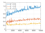
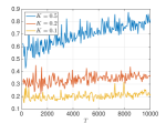
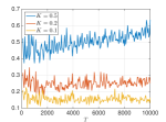
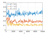
$\varphi=2.4$, $\epsilon=0.01$	$\varphi=2.6$, $\epsilon=0.01$	$\varphi=2.8$, $\epsilon=0.01$	$\varphi=3$, $\epsilon=0.01$
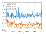
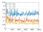
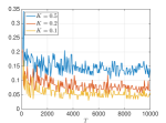
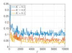
$\varphi=1.6$, $\epsilon=0.1$	$\varphi=1.8$, $\epsilon=0.1$	$\varphi=2$, $\epsilon=0.1$	$\varphi=2.2$, $\epsilon=0.01$
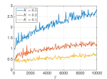
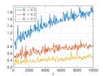
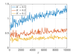
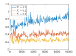
$\varphi=2.4$, $\epsilon=0.1$	$\varphi=2.6$, $\epsilon=0.1$	$\varphi=2.8$, $\epsilon=0.1$	$\varphi=3$, $\epsilon=0.01$

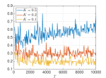
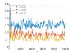
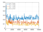
Appendix C S&P100 data

Table C1: S&P100 constituents.

Ticker	Name
AAPL	Apple Inc.	HPQ	Hewlett Packard Co.
ABT	Abbott Laboratories	IBM	International Business Machines
AEP	American Electric Power Co.	INTC	Intel Corporation
AIG	American International Group Inc.	JNJ	Johnson & Johnson Inc.
ALL	Allstate Corp.	JPM	JP Morgan Chase & Co.
AMGN	Amgen Inc.	KO	The Coca-Cola Company
AMZN	Amazon.com	LLY	Eli Lilly and Company
APA	Apache Corp.	LMT	Lockheed-Martin
APC	Anadarko Petroleum Corp.	LOW	Lowe’s
AXP	American Express Inc.	MCD	McDonald’s Corp.
BA	Boeing Co.	MDT	Medtronic Inc.
BAC	Bank of America Corp.	MMM	3M Company
BAX	Baxter International Inc.	MO	Altria Group
BK	Bank of New York	MRK	Merck & Co.
BMY	Bristol-Myers Squibb	MS	Morgan Stanley
BRK.B	Berkshire Hathaway	MSFT	Microsoft
C	Citigroup Inc.	NKE	Nike
CAT	Caterpillar Inc.	NOV	National Oilwell Varco
CL	Colgate-Palmolive Co.	NSC	Norfolk Southern Corp.
CMCSA	Comcast Corp.	ORCL	Oracle Corporation
COF	Capital One Financial Corp.	OXY	Occidental Petroleum Corp.
COP	ConocoPhillips	PEP	Pepsico Inc.
COST	Costco	PFE	Pfizer Inc.
CSCO	Cisco Systems	PG	Procter & Gamble Co.
CVS	CVS Caremark	QCOM	Qualcomm Inc.
CVX	Chevron	RTN	Raytheon Co.
DD	DuPont	SBUX	Starbucks Corporation
DELL	Dell	SLB	Schlumberger
DIS	The Walt Disney Company	SO	Southern Company
DOW	Dow Chemical	SPG	Simon Property Group, Inc.
DVN	Devon Energy	T	AT&T Inc.
EBAY	eBay Inc.	TGT	Target Corp.
EMC	EMC Corporation	TWX	Time Warner Inc.
EMR	Emerson Electric Co.	TXN	Texas Instruments
EXC	Exelon	UNH	UnitedHealth Group Inc.
F	Ford Motor	UNP	Union Pacific Corp.
FCX	Freeport-McMoran	UPS	United Parcel Service Inc.
FDX	FedEx	USB	US Bancorp
GD	General Dynamics	UTX	United Technologies Corp.
GE	General Electric Co.	VZ	Verizon Communications Inc.
GILD	Gilead Sciences	WAG	Walgreens
GS	Goldman Sachs	WFC	Wells Fargo
HAL	Halliburton	WMB	Williams Companies
HD	Home Depot	WMT	Wal-Mart
HON	Honeywell	XOM	Exxon Mobil Corp.

Appendix D Additional simulation results

Table D1: Simulation results. Common components. Values of the bandwidths are: $B_{T}=5$ and $M_{T}=5$ for all $T$.

$q=1$, $Q=1$
		$T=200$		$T=500$		$T=1000$
		$n=100$	$n=200$	$n=100$	$n=200$	$n=100$	$n=200$
$MSE^{X}$		0.089	0.091	0.073	0.075	0.061	0.064
$MSE^{\chi}$	$\kappa_{T}=0$	0.450	0.412	0.630	0.607	0.793	0.734
$MSE^{\chi}$	$\kappa_{T}=0.2$	0.469	0.448	0.673	0.641	0.750	0.730
$MSE^{\chi}$	$\kappa_{T}=0.4$	0.455	0.477	0.671	0.672	0.788	0.820
$MAD^{X}$		0.184	0.167	0.176	0.158	0.170	0.157
$MAD^{\chi}$	$\kappa_{T}=0$	0.486	0.458	0.575	0.555	0.650	0.619
$MAD^{\chi}$	$\kappa_{T}=0.2$	0.491	0.468	0.591	0.563	0.620	0.608
$MAD^{\chi}$	$\kappa_{T}=0.4$	0.481	0.487	0.583	0.579	0.630	0.637
$MAX^{X}$		9.016	10.336	11.809	10.955	11.742	16.046
$MAX^{\chi}$	$\kappa_{T}=0$	11.385	19.027	18.554	40.420	55.108	50.038
$MAX^{\chi}$	$\kappa_{T}=0.2$	18.154	29.037	34.038	37.224	45.037	61.851
$MAX^{\chi}$	$\kappa_{T}=0.4$	20.399	23.017	33.477	44.226	65.348	51.665
$q=3$, $Q=2$
		$T=200$		$T=500$		$T=1000$
		$n=100$	$n=200$	$n=100$	$n=200$	$n=100$	$n=200$
$MSE^{X}$		0.091	0.096	0.067	0.070	0.056	0.058
$MSE^{\chi}$	$\kappa_{T}=0$	0.361	0.277	0.373	0.259	0.420	0.257
$MSE^{\chi}$	$\kappa_{T}=0.2$	0.316	0.232	0.340	0.336	0.229	0.225
$MSE^{\chi}$	$\kappa_{T}=0.4$	0.300	0.226	0.305	0.210	0.319	0.218
$MAD^{X}$		0.213	0.205	0.186	0.183	0.175	0.172
$MAD^{\chi}$	$\kappa_{T}=0$	0.458	0.395	0.461	0.380	0.489	0.376
$MAD^{\chi}$	$\kappa_{T}=0.2$	0.426	0.359	0.439	0.432	0.354	0.350
$MAD^{\chi}$	$\kappa_{T}=0.4$	0.413	0.354	0.413	0.338	0.421	0.344
$MAX^{X}$		5.632	8.485	12.693	8.876	11.027	13.225
$MAX^{\chi}$	$\kappa_{T}=0$	5.151	4.585	5.254	6.031	7.377	5.736
$MAX^{\chi}$	$\kappa_{T}=0.2$	3.897	4.985	4.981	6.400	5.038	6.491
$MAX^{\chi}$	$\kappa_{T}=0.4$	5.855	4.454	7.723	7.237	5.837	5.723
$q=2$, $Q=3$
		$T=200$		$T=500$		$T=1000$
		$n=100$	$n=200$	$n=100$	$n=200$	$n=100$	$n=200$
$MSE^{X}$		0.087	0.088	0.068	0.071	0.056	0.064
$MSE^{\chi}$	$\kappa_{T}=0$	0.355	0.300	0.384	0.274	0.425	0.280
$MSE^{\chi}$	$\kappa_{T}=0.2$	0.327	0.265	0.347	0.236	0.380	0.231
$MSE^{\chi}$	$\kappa_{T}=0.4$	0.300	0.247	0.315	0.208	0.361	0.215
$MAD^{X}$		0.210	0.204	0.191	0.187	0.177	0.180
$MAD^{\chi}$	$\kappa_{T}=0$	0.459	0.419	0.475	0.396	0.496	0.399
$MAD^{\chi}$	$\kappa_{T}=0.2$	0.439	0.391	0.450	0.366	0.469	0.361
$MAD^{\chi}$	$\kappa_{T}=0.4$	0.420	0.376	0.427	0.343	0.456	0.347
$MAX^{X}$		9.532	9.098	6.292	11.581	8.078	7.409
$MAX^{\chi}$	$\kappa_{T}=0$	3.978	4.204	4.184	5.321	6.107	5.417
$MAX^{\chi}$	$\kappa_{T}=0.2$	3.986	4.835	4.913	5.932	5.512	7.808
$MAX^{\chi}$	$\kappa_{T}=0.4$	4.524	4.674	4.521	6.284	5.944	5.705

Table D2: Simulation results. Empirical coverage and frequency of confidence bound violations averaged over all $n$ series and all $\mathcal{M}$ replications, when $T=1000$ and $\mathcal{M}=200$. Values of the bandwidths are: $B_{T}=5$ and $M_{T}=5$ for all $T$.

$q=1$, $Q=1$
		$n=100$					$n=200$
		$\alpha$					$\alpha$
		0.32	0.2	0.1	0.05	0.01	0.32	0.2	0.1	0.05	0.01
$C(\alpha)$	$\kappa_{T}=0$	0.6854	0.8098	0.9099	0.9581	0.9928	0.6793	0.7871	0.8809	0.9335	0.9831
$V_{+}(\alpha/2)$		0.1573	0.0951	0.0441	0.0217	0.0040	0.1606	0.1055	0.0599	0.0332	0.0087
$V_{-}(\alpha/2)$		0.1573	0.0951	0.0460	0.0202	0.0032	0.1601	0.1074	0.0593	0.0333	0.0083
$C(\alpha)$	$\kappa_{T}=0.2$	0.7046	0.7982	0.8790	0.9246	0.9744	0.7126	0.8207	0.9070	0.9490	0.9841
$V_{+}(\alpha/2)$		0.1465	0.0992	0.0594	0.0373	0.0129	0.1439	0.0891	0.0461	0.0247	0.0081
$V_{-}(\alpha/2)$		0.1489	0.1026	0.0616	0.0381	0.0127	0.1436	0.0902	0.0469	0.0264	0.0078
$C(\alpha)$	$\kappa_{T}=0.4$	0.7531	0.8440	0.9197	0.9543	0.9845	0.7687	0.8511	0.9243	0.9628	0.9969
$V_{+}(\alpha/2)$		0.1217	0.0759	0.0401	0.0229	0.0084	0.1171	0.0775	0.0406	0.0201	0.0017
$V_{-}(\alpha/2)$		0.1252	0.0801	0.0402	0.0228	0.0071	0.1142	0.0714	0.0351	0.0172	0.0014
$q=3$, $Q=2$
		$n=100$					$n=200$
		$\alpha$					$\alpha$
		0.32	0.2	0.1	0.05	0.01	0.32	0.2	0.1	0.05	0.01
$C(\alpha)$	$\kappa_{T}=0$	0.6821	0.7978	0.8907	0.9405	0.9800	0.6651	0.7872	0.8903	0.9445	0.9840
$V_{+}(\alpha/2)$		0.1596	0.1003	0.0556	0.0294	0.0097	0.1596	0.1003	0.0556	0.0294	0.0097
$V_{-}(\alpha/2)$		0.1583	0.1019	0.0537	0.0301	0.0103	0.1583	0.1019	0.0537	0.0301	0.0103
$C(\alpha)$	$\kappa_{T}=0.2$	0.6837	0.7787	0.8609	0.9089	0.9602	0.7277	0.8290	0.9124	0.9552	0.9910
$V_{+}(\alpha/2)$		0.1560	0.1097	0.0689	0.0442	0.0186	0.1387	0.0865	0.0442	0.0220	0.0037
$V_{-}(\alpha/2)$		0.1603	0.1116	0.0702	0.0469	0.0212	0.1336	0.0846	0.0435	0.0229	0.0054
$C(\alpha)$	$\kappa_{T}=0.4$	0.7500	0.8369	0.9141	0.9527	0.9881	0.7551	0.8431	0.9149	0.9543	0.9915
$V_{+}(\alpha/2)$		0.1217	0.0794	0.0419	0.0233	0.0059	0.1232	0.0782	0.0409	0.0219	0.0036
$V_{-}(\alpha/2)$		0.1283	0.0837	0.0440	0.0240	0.0060	0.1218	0.0788	0.0442	0.0238	0.0049
$q=2$, $Q=3$
		$n=100$					$n=200$
		$\alpha$					$\alpha$
		0.32	0.2	0.1	0.05	0.01	0.32	0.2	0.1	0.05	0.01
$C(\alpha)$	$\kappa_{T}=0$	0.6137	0.7191	0.8259	0.8916	0.9598	0.6631	0.7803	0.8820	0.9393	0.9866
$V_{+}(\alpha/2)$		0.2034	0.1490	0.0894	0.0552	0.0217	0.1722	0.1118	0.0610	0.0317	0.0078
$V_{-}(\alpha/2)$		0.1829	0.1319	0.0847	0.0532	0.0185	0.1648	0.1080	0.0571	0.0290	0.0057
$C(\alpha)$	$\kappa_{T}=0.2$	0.7166	0.8219	0.9095	0.9549	0.9925	0.7259	0.8332	0.9262	0.9660	0.9941
$V_{+}(\alpha/2)$		0.1495	0.0940	0.0493	0.0252	0.0040	0.1371	0.0826	0.0372	0.0176	0.0029
$V_{-}(\alpha/2)$		0.1339	0.0841	0.0412	0.0199	0.0035	0.1371	0.0843	0.0367	0.0164	0.0031
$C(\alpha)$	$\kappa_{T}=0.4$	0.7715	0.8569	0.9282	0.9671	0.9950	0.7265	0.8165	0.8986	0.9466	0.9918
$V_{+}(\alpha/2)$		0.1146	0.0728	0.0361	0.0149	0.0019	0.1232	0.0782	0.0409	0.0219	0.0036
$V_{-}(\alpha/2)$		0.1139	0.0703	0.0357	0.0180	0.0031	0.1218	0.07878	0.0442	0.0238	0.0049

Table D3: Simulation results. Common components. Values of the bandwidths are: $B_{T}=1$ and $M_{T}=14$ for $T=200$; $B_{T}=1$ and $M_{T}=22$ for $T=500$; $B_{T}=1$ and $M_{T}=31$ for $T=1000$.

$q=1$, $Q=1$
		$T=200$		$T=500$		$T=1000$
		$n=100$	$n=200$	$n=100$	$n=200$	$n=100$	$n=200$
$MSE^{X}$		0.467	4.568	0.334	0.344	0.271	0.251
$MSE^{\chi}$	$\kappa_{T}=0$	0.547	0.508	0.477	0.422	0.419	0.343
$MSE^{\chi}$	$\kappa_{T}=0.2$	0.561	0.527	0.481	0.427	0.412	0.331
$MSE^{\chi}$	$\kappa_{T}=0.4$	0.593	0.487	0.405	0.560	0.458	0.350
$MAD^{X}$		0.417	0.386	0.366	0.330	0.337	0.294
$MAD^{\chi}$	$\kappa_{T}=0$	0.555	0.524	0.508	0.467	0.471	0.417
$MAD^{\chi}$	$\kappa_{T}=0.2$	0.556	0.526	0.503	0.460	0.459	0.399
$MAD^{\chi}$	$\kappa_{T}=0.4$	0.573	0.502	0.448	0.541	0.472	0.406
$MAX^{X}$		36.332	826.833	20.032	39.123	31.799	46.432
$MAX^{\chi}$	$\kappa_{T}=0$	7.023	8.756	7.328	8.536	8.251	8.111
$MAX^{\chi}$	$\kappa_{T}=0.2$	8.059	8.743	7.758	9.147	9.171	8.843
$MAX^{\chi}$	$\kappa_{T}=0.4$	8.727	9.109	9.846	9.310	9.387	9.895
$q=3$, $Q=2$
		$T=200$		$T=500$		$T=1000$
		$n=100$	$n=200$	$n=100$	$n=200$	$n=100$	$n=200$
$MSE^{X}$		0.255	0.250	0.159	0.157	0.116	0.121
$MSE^{\chi}$	$\kappa_{T}=0$	0.389	0.375	0.299	0.273	0.248	0.234
$MSE^{\chi}$	$\kappa_{T}=0.2$	0.369	0.268	0.212	0.360	0.241	0.202
$MSE^{\chi}$	$\kappa_{T}=0.4$	0.358	0.358	0.250	0.252	0.191	0.176
$MAD^{X}$		0.357	0.337	0.284	0.272	0.248	0.245
$MAD^{\chi}$	$\kappa_{T}=0$	0.480	0.467	0.417	0.395	0.380	0.365
$MAD^{\chi}$	$\kappa_{T}=0.2$	0.465	0.391	0.348	0.454	0.367	0.334
$MAD^{\chi}$	$\kappa_{T}=0.4$	0.457	0.450	0.376	0.372	0.328	0.311
$MAX^{X}$		8.732	10.161	10.535	11.145	12.495	13.895
$MAX^{\chi}$	$\kappa_{T}=0$	5.721	5.525	5.010	5.412	4.532	5.946
$MAX^{\chi}$	$\kappa_{T}=0.2$	6.036	5.137	4.693	5.637	5.194	6.250
$MAX^{\chi}$	$\kappa_{T}=0.4$	5.332	5.653	5.659	6.776	5.285	7.061
$q=2$, $Q=3$
		$T=200$		$T=500$		$T=1000$
		$n=100$	$n=200$	$n=100$	$n=200$	$n=100$	$n=200$
$MSE^{X}$		0.298	0.286	0.194	0.184	0.134	0.143
$MSE^{\chi}$	$\kappa_{T}=0$	0.480	0.439	0.387	0.353	0.311	0.300
$MSE^{\chi}$	$\kappa_{T}=0.2$	0.463	0.426	0.358	0.327	0.277	0.266
$MSE^{\chi}$	$\kappa_{T}=0.4$	0.464	0.453	0.352	0.341	0.271	0.247
$MAD^{X}$		0.393	0.370	0.316	0.303	0.267	0.272
$MAD^{\chi}$	$\kappa_{T}=0$	0.538	0.511	0.478	0.453	0.428	0.417
$MAD^{\chi}$	$\kappa_{T}=0.2$	0.526	0.500	0.455	0.432	0.400	0.388
$MAD^{\chi}$	$\kappa_{T}=0.4$	0.525	0.515	0.449	0.438	0.392	0.372
$MAX^{X}$		9.353	10.260	8.710	14.061	9.802	12.255
$MAX^{\chi}$	$\kappa_{T}=0$	6.081	5.367	5.962	6.078	5.683	7.025
$MAX^{\chi}$	$\kappa_{T}=0.2$	5.417	5.818	6.051	6.590	6.481	7.808
$MAX^{\chi}$	$\kappa_{T}=0.4$	5.905	6.056	5.951	7.419	6.519	6.513

Table D4: Simulation results. Empirical coverage and frequency of confidence bound violations averaged over all $n$ series and all $\mathcal{M}$ replications, for $T=1000$ and $\mathcal{M}=200$. Values of the bandwidths are: $B_{T}=1$ and $M_{T}=14$ for $T=200$; $B_{T}=1$ and $M_{T}=22$ for $T=500$; $B_{T}=1$ and $M_{T}=31$ for $T=1000$.

$q=1$, $Q=1$
		$n=100$					$n=200$
		$\alpha$					$\alpha$
		0.32	0.2	0.1	0.05	0.01	0.32	0.2	0.1	0.05	0.01
$C(\alpha)$	$\kappa_{T}=0$	0.7211	0.8374	0.9267	0.9708	0.9966	0.6287	0.7476	0.8602	0.9238	0.9856
$V_{+}(\alpha/2)$		0.1460	0.0855	0.0393	0.0144	0.0020	0.1883	0.1285	0.0703	0.0394	0.0072
$V_{-}(\alpha/2)$		0.1329	0.0771	0.0340	0.0148	0.0014	0.1831	0.1240	0.0696	0.0368	0.0073
$C(\alpha)$	$\kappa_{T}=0.2$	0.7615	0.8597	0.9367	0.9763	0.9975	0.6841	0.7864	0.8846	0.9346	0.9882
$V_{+}(\alpha/2)$		0.1255	0.0730	0.0332	0.0125	0.0011	0.1603	0.1090	0.0585	0.0335	0.0057
$V_{-}(\alpha/2)$		0.1130	0.0673	0.0301	0.0112	0.0014	0.1557	0.1047	0.0570	0.0320	0.0062
$C(\alpha)$	$\kappa_{T}=0.4$	0.7747	0.8623	0.9368	0.9708	0.9966	0.6957	0.7856	0.8735	0.9272	0.9821
$V_{+}(\alpha/2)$		0.1135	0.0678	0.0291	0.0133	0.0012	0.1495	0.1060	0.0623	0.0358	0.0081
$V_{-}(\alpha/2)$		0.1118	0.0699	0.0341	0.0160	0.0014	0.1549	0.1085	0.0642	0.0371	0.0099
$q=3$, $Q=2$
		$n=100$					$n=200$
		$\alpha$					$\alpha$
		0.32	0.2	0.1	0.05	0.01	0.32	0.2	0.1	0.05	0.01
$C(\alpha)$	$\kappa_{T}=0$	0.6826	0.8013	0.9040	0.9551	0.9942	0.6327	0.7474	0.8486	0.9090	0.9706
$V_{+}(\alpha/2)$		0.1552	0.1001	0.0472	0.0229	0.0027	0.1847	0.1263	0.0752	0.0450	0.0142
$V_{-}(\alpha/2)$		0.1622	0.0986	0.0488	0.0220	0.0031	0.1826	0.1264	0.0763	0.0461	0.0153
$C(\alpha)$	$\kappa_{T}=0.2$	0.7226	0.8271	0.9171	0.9594	0.9941	0.6749	0.7732	0.8639	0.9157	0.9720
$V_{+}(\alpha/2)$		0.1362	0.0869	0.0410	0.0209	0.0031	0.1636	0.1134	0.0672	0.0415	0.0135
$V_{-}(\alpha/2)$		0.1412	0.0860	0.0419	0.0197	0.0028	0.1616	0.1135	0.0690	0.0428	0.0146
$C(\alpha)$	$\kappa_{T}=0.4$	0.7322	0.8250	0.9036	0.9437	0.9850	0.7239	0.8100	0.8913	0.9335	0.9766
$V_{+}(\alpha/2)$		0.1321	0.0854	0.0470	0.0259	0.0068	0.1392	0.0960	0.0539	0.0333	0.0121
$V_{-}(\alpha/2)$		0.1357	0.0896	0.0494	0.0304	0.0082	0.1370	0.0941	0.0549	0.0333	0.0114
$q=2$, $Q=3$
		$n=100$					$n=200$
		$\alpha$					$\alpha$
		0.32	0.2	0.1	0.05	0.01	0.32	0.2	0.1	0.05	0.01
$C(\alpha)$	$\kappa_{T}=0$	0.6604	0.7730	0.8773	0.9312	0.9767	0.6973	0.8141	0.9118	0.9582	0.9946
$V_{+}(\alpha/2)$		0.1682	0.1107	0.0595	0.0314	0.0108	0.1481	0.0901	0.0424	0.0204	0.0029
$V_{-}(\alpha/2)$		0.1714	0.1163	0.0632	0.0374	0.0125	0.1547	0.0959	0.0458	0.0215	0.0026
$C(\alpha)$	$\kappa_{T}=0.2$	0.6979	0.8006	0.8899	0.9367	0.9794	0.7446	0.8415	0.9240	0.9647	0.9959
$V_{+}(\alpha/2)$		0.1507	0.0973	0.0521	0.0288	0.0100	0.1256	0.0759	0.0365	0.0168	0.0022
$V_{-}(\alpha/2)$		0.1514	0.1021	0.0580	0.0345	0.0106	0.1298	0.0827	0.0396	0.0186	0.0020
$C(\alpha)$	$\kappa_{T}=0.4$	0.7368	0.8290	0.9009	0.9462	0.9887	0.7557	0.8420	0.9160	0.9566	0.9902
$V_{+}(\alpha/2)$		0.1316	0.0864	0.0501	0.0259	0.0056	0.1273	0.0834	0.0434	0.0219	0.0047
$V_{-}(\alpha/2)$		0.1316	0.0846	0.0490	0.0279	0.0057	0.1171	0.0747	0.0407	0.0216	0.0051

References

- Aït-Sahalia and Xiu, (2017) Aït-Sahalia, Y. and Xiu, D. (2017). Using principal component analysis to estimate a high dimensional factor model with high-frequency data. Journal of Econometrics, 201:384–399.
- Alizadeh et al., (2002) Alizadeh, S., Brandt, M. W., and Diebold, F. X. (2002). Range-based estimation of stochastic volatility models. The Journal of Finance, 57:1047–1091.
- Anderson and Deistler, (2008) Anderson, B. D. and Deistler, M. (2008). Generalized linear dynamic factor models. A structure theory. In 47th IEEE Conference on Decision and Control.
- Asai et al., (2006) Asai, M., McAleer, M., and Yu, J. (2006). Multivariate stochastic volatility: A review. Econometric Reviews, 25:145–175.
- Bai and Ng, (2002) Bai, J. and Ng, S. (2002). Determining the number of factors in approximate factor models. Econometrica, 70:191–221.
- Bai and Ng, (2008) Bai, J. and Ng, S. (2008). Forecasting economic time series using targeted predictors. Journal of Econometrics, 146:304–317.
- Barigozzi and Hallin, (2016) Barigozzi, M. and Hallin, M. (2016). General dynamic factors and volatilities: Recovering the market volatility shocks. The Econometrics Journal, 19:C33–C60.
- (8) Barigozzi, M. and Hallin, M. (2017a). General dynamic factors and volatilities: Estimation and forecasting. Journal of Econometrics, 201:307–321.
- (9) Barigozzi, M. and Hallin, M. (2017b). Networks, dynamic factors, and the volatility analysis of high-dimensional financial series. Journal of the Royal Statistical Society, Series C, 66:581–605.
- Barigozzi et al., (2018) Barigozzi, M., Hallin, M., and Soccorsi, S. (2018). Identification of global and local shocks in international financial markets via general dynamic factor models. Journal of Financial Econometrics. available online.
- Bauwens et al., (2006) Bauwens, L., Laurent, S., and Rombouts, J. V. K. (2006). Multivariate GARCH models: A survey. Journal of the Applied Econometrics, 21:79–109.
- Boivin and Ng, (2006) Boivin, J. and Ng, S. (2006). Are more data always better for factor analysis? Journal of Econometrics, 127:169–194.
- Borovkov, (2000) Borovkov, A. A. (2000). Large deviation probabilities for random walks with semiexponential distributions. Siberian Mathematical Journal, 41:1061–1093.
- Brillinger, (2001) Brillinger, D. (2001). Time Series: Data Analysis and Theory. Classics in Applied Mathematics. Society for Industrial and Applied Mathematics.
- Chamberlain and Rothschild, (1983) Chamberlain, G. and Rothschild, M. (1983). Arbitrage, factor structure, and mean–variance analysis on large asset markets. Econometrica, 51:1281–304.
- Chicheportiche and Bouchaud, (2015) Chicheportiche, R. and Bouchaud, J.-P. (2015). A nested factor model for non-linear dependencies in stock returns. Quantitative Finance, 15:1789–1804.
- Christoffersen, (1998) Christoffersen, P. F. (1998). Evaluating interval forecasts. International Economic Review, 39:841–862.
- Connor and Korajczyk, (1993) Connor, G. and Korajczyk, R. A. (1993). A test for the number of factors in an approximate factor model. the Journal of Finance, 48:1263–1291.
- Connor et al., (2006) Connor, G., Korajczyk, R. A., and Linton, O. (2006). The common and specific components of dynamic volatility. Journal of Econometrics, 132:231–255.
- Davidson, (1994) Davidson, J. (1994). Stochastic Limit Theory: An Introduction for Econometricians. Oxford University Press.
- den Haan and Levin, (1997) den Haan, W. J. and Levin, A. T. (1997). A practitioner’s guide to robust covariance matrix estimation. In Robust Inference, volume 15 of Handbook of Statistics. Elsevier.
- Diebold and Nerlove, (1989) Diebold, F. X. and Nerlove, M. (1989). The dynamics of exchange rate volatility: a multivariate latent factor ARCH model. Journal of Applied Econometrics, 4:1–21.
- Dufour et al., (1998) Dufour, J., Hallin, M., and Mizera, I. (1998). Generalized run tests for heteroscedastic time series. Journal of Nonparametric Statistics, 9:39–86.
- Engle and Marcucci, (2006) Engle, R. F. and Marcucci, J. (2006). A long–run pure variance common features model for the common volatilities of the Dow Jones. Journal of Econometrics, 132:7–42.
- Fan et al., (2013) Fan, J., Liao, Y., and Mincheva, M. (2013). Large covariance estimation by thresholding principal orthogonal complements. Journal of the Royal Statistical Society, Series B, 75:603–680.
- Fan et al., (2015) Fan, J., Liao, Y., and Shi, X. (2015). Risks of large portfolios. Journal of Econometrics, 186:367–387.
- Forni et al., (2009) Forni, M., Giannone, D., Lippi, M., and Reichlin, L. (2009). Opening the black box: Structural factor models versus structural VARs. Econometric Theory, 25:1319–1347.
- Forni et al., (2018) Forni, M., Giovannelli, A., Lippi, M., and Soccorsi, S. (2018). Dynamic factor model with infinite-dimensional factor space: Forecasting. Journal of Applied Econometrics, 33:625–642.
- Forni et al., (2000) Forni, M., Hallin, M., Lippi, M., and Reichlin, L. (2000). The generalized dynamic factor model: Identification and estimation. The Review of Economics and Statistics, 82:540–554.
- Forni et al., (2015) Forni, M., Hallin, M., Lippi, M., and Zaffaroni, P. (2015). Dynamic factor models with infinite-dimensional factor spaces: One-sided representations. Journal of Econometrics, 185:359–371.
- Forni et al., (2017) Forni, M., Hallin, M., Lippi, M., and Zaffaroni, P. (2017). Dynamic factor models with infinite dimensional factor space: Asymptotic analysis. Journal of Econometrics, 199:74–92.
- Forni and Lippi, (2001) Forni, M. and Lippi, M. (2001). The generalized dynamic factor model: Representation theory. Econometric Theory, 17:1113–1141.
- Forni and Lippi, (2011) Forni, M. and Lippi, M. (2011). The unrestricted dynamic factor model: One-sided representation results. Journal of Econometrics, 163:23–28.
- Francq and Zakoian, (2011) Francq, C. and Zakoian, J.-M. (2011). GARCH Models: Structure, Statistical Inference and Financial Applications. John Wiley & Sons.
- Francq and Zakoian, (2019) Francq, C. and Zakoian, J.-M. (2019). Virtual Historical Simulation for estimating the conditional VaR of large portfolios. mimeo.
- Hallin and Lippi, (2013) Hallin, M. and Lippi, M. (2013). Factor models in high–dimensional time series. A time-domain approach. Stochastic Processes and their Applications, 123:2678–2695.
- Hallin and Liška, (2007) Hallin, M. and Liška, R. (2007). Determining the number of factors in the general dynamic factor model. Journal of the American Statistical Association, 102:603–617.
- Hamilton, (1994) Hamilton, J. D. (1994). Time series analysis. Princeton University Press.
- Hannan, (1970) Hannan, E. J. (1970). Multiple Time Series. John Wiley & Sons.
- Harvey et al., (1992) Harvey, A., Ruiz, E., and Sentana, E. (1992). Unobserved component time series models with arch disturbances. Journal of Econometrics, 52:129–157.
- Jurado et al., (2015) Jurado, K., Ludvigson, S. C., and Ng, S. (2015). Measuring uncertainty. American Economic Review, 105:1177–1216.
- Kuchibhotla and Chakrabortty, (2018) Kuchibhotla, A. K. and Chakrabortty, A. (2018). Moving beyond sub-gaussianity in high dimensional statistics: Applications in covariance matrix estimation and linear regressions. arXiv preprint arXiv:1804.02605.
- Lütkepohl, (2005) Lütkepohl, H. (2005). New Introduction to Multiple Time Series Analysis. Springer Science & Business Media.
- McNemar, (1947) McNemar, Q. M. (1947). Note on the sampling error of the difference between correlated proportions or percentages. Psychometrika, 12:153–157.
- Merlevède et al., (2011) Merlevède, F., Peligrad, M., and Rio, E. (2011). A bernstein type inequality and moderate deviations for weakly dependent sequences. Probability Theory and Related Fields, 151:435–474.
- Ng et al., (1992) Ng, V., Engle, R. F., and Rothschild, M. (1992). A multi-dynamic-factor model for stock returns. Journal of Econometrics, 52:245–266.
- Parzen, (1957) Parzen, E. (1957). On consistent estimates of the spectrum of a stationary time series. The Annals of Mathematical Statistics, 28:329–348.
- Peña and Box, (1987) Peña, D. and Box, G. E. (1987). Identifying a simplifying structure in time series. Journal of the American statistical Association, 82:836–843.
- Priestley, (2001) Priestley, M. B. (2001). Spectral Analysis and Time Series. Elsevier Academic Press.
- Sentana et al., (2008) Sentana, E., Calzolari, G., and Fiorentini, G. (2008). Indirect estimation of large conditionally heteroskedastic factor models, with an application to the Dow 30 stocks. Journal of Econometrics, 146:10–25.
- Stock and Watson, (2002) Stock, J. H. and Watson, M. W. (2002). Forecasting using principal components from a large number of predictors. Journal of the American Statistical Association, 97:1167–1179.
- Tiao, (1972) Tiao, G. C. (1972). Asymptotic behaviour of temporal aggregates of time series. Biometrika, 59:525–531.
- Tiao and Box, (1981) Tiao, G. C. and Box, G. E. (1981). Modeling multiple time series with applications. Journal of the American Statistical Association, 76:802–816.
- Tiao and Guttman, (1980) Tiao, G. C. and Guttman, I. (1980). Forecasting contemporal aggregates of multiple time series. Journal of Econometrics, 12:219–230.
- Tiao and Hillmer, (1978) Tiao, G. C. and Hillmer, S. C. (1978). Some consideration of decomposition of a time series. Biometrika, 65:497–502.
- Tiao and Tsay, (1989) Tiao, G. C. and Tsay, R. S. (1989). Model specification in multivariate time series. Journal of the Royal Statistical Society: Series B (Methodological), 51:157–195.
- Trucíos et al., (2019) Trucíos, . C., Mazzeu, J., Hallin, M., Zevallos, M., Hotta, L., and Pereira, P. V. (2019). Forecasting conditional covariance matrices in high-dimensional time series with application to dynamic portfolio optimization: a general dynamic factor approach. Technical Report DOI: 10.13140/RG.2.2.23950.82241, ECARES.
- Tsay and Tiao, (1985) Tsay, R. S. and Tiao, G. C. (1985). Use of canonical analysis in time series model identification. Biometrika, 72:299–315.
- Uchaikin and Zolotarev, (2011) Uchaikin, V. V. and Zolotarev, V. M. (2011). Chance and Stability: Stable Distributions and their Applications. Walter de Gruyter.
- Vershynin, (2012) Vershynin, R. (2012). Introduction to the non-asymptotic analysis of random matrices. In Eldar, Y. and Kutyniok, G., editors, Compressed Sensing. Theory and Applications. Cambridge University Press.
- Vladimirova and Arbel, (2019) Vladimirova, M. and Arbel, J. (2019). Sub-Weibull distributions: generalizing sub-Gaussian and sub-Exponential properties to heavier-tailed distributions. arXiv preprint arXiv:1905.04955.
- Weyl, (1912) Weyl, H. (1912). Das asymptotische Verteilungsgesetz der Eigenwerte linearer partieller Differentialgleichungen. Mathematische Annalen, 71:441–479.
- Wu and Zaffaroni, (2018) Wu, W. B. and Zaffaroni, P. (2018). Asymptotic theory for spectral density estimates of general multivariate time series. Econometric Theory, 34:1–22.