On the stability of the Couette-Taylor flow between rotating porous cylinders with radial flow

Abstract

We study the stability of the Couette-Taylor flow between porous cylinders with radial throughflow. It had been shown earlier that this flow can be unstable with respect to non-axisymmetric (azimuthal or helical) waves provided that the radial Reynolds number, $R$ (constructed using the radial velocity at the inner cylinder and its radius), is high. In this paper, we present a very detailed and, in many respects, novel chart of critical curves in a region of moderate values of $R$, and we show that, starting from values of $R$, as low as $10$, the critical modes inherited from the inviscid instability gradually substitute the classical Taylor vortices. Also, we have looked more closely at the effect of a weak radial flow (relatively low $R$) on the Taylor instability and found that a radial flow directed from the inner cylinder to the outer one is capable of stabilizing the Couette-Taylor flow provided that the gap between the cylinders is wide enough. This observation is in a sharp contrast with the case of relatively narrow gaps for which the opposite effect is well-known.

1 Introduction

We study the linear stability of a steady viscous incompressible flow in a gap between two rotating porous cylinders with a radial flow. The governing parameters of the flow are the radial Reynolds number, $R$ (constructed using the radial velocity at the inner cylinder and its radius), and two azimuthal Reynolds numbers, $\mbox{{Re}}_{1}$ and $\mbox{{Re}}_{2}$ (based on the azimuthal velocities of the inner and outer cylinders, respectively, and the gap between the cylinders). The velocity of the basic flow has nonzero azimuthal and radial components and zero axial component. It is a straightforward generalisation of the classical Couette-Taylor flow to the case when a radial flow is present. The direction of the radial flow can be from the inner cylinder to the outer one (the diverging flow) or from the outer cylinder to the inner one (the converging flow). The most interesting feature of the basic flow is that the azimuthal velocity profile non-trivially depends on the radial Reynolds number $R$. In particular, for high radial Reynolds numbers, it becomes irrotational everywhere except for a thin boundary layer near the outflow part of the boundary (i.e. near the outer cylinder for the diverging flow or near the inner cylinder for the converging flow).

The stability of the Couette-Taylor flow with a radial throughflow had been studied by many authors (e.g., [3, 8, 34, 28, 27, 37, 31, 32]). Most studies were motivated by applications to dynamic filtration devices (see, e.g., [39, 4]) and vortex flow reactors (see [17] and references therein). Recently, it was also argued by Gallet et al. [15] and Kerswell [26] that such flows may have some relevance to astrophysical flows in accretion discs (see also [25]). These possible applications make it important to better understand the structure and the stability properties of the Couette-Taylor flow with radial flow not only for flow regimes specific to a particular application or a device, but also for a much wider range of the governing parameters of the problem.

One of the main aims of early papers (e.g., [3, 34, 28]) was to determine the effect of the radial flow on the stability of the circular Couette-Taylor flow to axisymmetric perturbations, and the common conclusion was that both a converging radial flow and a sufficiently strong diverging flow have a stabilizing effect on the Taylor instability, but when a diverging flow is weak, it has a destabilizing effect [34, 24, 28]. We note in passing that we have found that, when the cylinders rotate in opposite directions, the destabilising effect of a weak diverging flow occurs for all values of the gap between the cylinders; however, when the outer cylinder is not rotating, a weak diverging flow has a destabilising effect, but only if the gap between the cylinders is relatively small, and it has a stabilising effect if the gap is sufficiently large (see section 3.2 of the present paper). The question that remained open was whether a radial flow itself can induce instability for flows which are stable without it. This question had been answered affirmatively by Fujita et al. [13] and later by Gallet et al. [15] who had demonstrated that particular classes of viscous flows between porous rotating cylinders can be unstable to small two-dimensional perturbations. Later it had been shown in [21] that both converging and diverging inviscid irrotational flows can be linearly unstable to two-dimensional perturbations and that the instability persists for high, but finite radial Reynolds numbers. In [22], it had been shown that not only the particular examples of viscous steady flows considered in [15, 21] can be unstable to two-dimensional perturbations, but this is also true for much wider classes of both converging and diverging flows. Further development of the two-dimensional theory can be found in a recent paper by Kerswell [26] where, among other things, the effects of compressibility, three-dimensionality and nonlinearity have been considered. Kerswell has also pointed to a similarity between the instability induced by the radial flow and the so-called stratorotational instability (SRI) which is due to the axial density stratification in the Couette-Taylor flow (see also [16, 30]). The effect of three-dimensionality has been also studied in [23], where it has been shown that the basic flow is unstable provided that the radial Reynolds number is sufficiently high and that, in almost all cases, the most unstable mode is two-dimensional, but never axisymmetric. Finally, in a recent paper, Martinand et al [32] have studied the stability of the Couette-Taylor flow between porous cylinders with both radial and axial flows. Among other things, they have found that the critical mode becomes non-axisymmetric when the radial flow is sufficiently strong and the gap between the cylinders is sufficiently wide.

Even though the above papers resulted in a considerable progress in our understanding of the effect of a radial flow on the stability of the Couette-Taylor flow, the full picture is still not very clear, because of various restrictions that have been imposed either on the perturbations or on the basic flow. The aim of the present paper is to fill most of the existing gaps in the linear stability analysis and to obtain theoretical linear stability diagram similar to the diagram of Andereck et al. [1] that summarises the experimental results on the classical Couette-Taylor flow.

We shall pay particular attention to the inviscid instability studied in [21, 22, 26, 23]. It was argued in [23] that the instability occurs because adding a radial flow to a circular flow between cylinders radically changes the inviscid stability problem. One may think of the radial flow as a singular perturbation of the flow with circular streamlines. It is therefore not completely unexpected that adding the radial flow results in the appearance of new unstable inviscid modes which do not exist in the absence of the radial flow. This is somewhat similar to the tearing instability in the magnetohydrodynamics, where the unstable tearing mode appears when a small resistivity is added (see, e.g., [14]). It had been shown in [23] that the inviscid instability persists for viscous flows, provided that the radial Reynolds number is sufficiently high. For possible applications, it is necessary to know whether this instability can survive for relatively low $R$, and an answer to this question, which itself is important, is the essential step towards our main aim.

The outline of the paper is as follows. In Section 2, we state the governing equations, the basic flow and the linearised stability problem. Section 3 describes the results of the linear stability analysis. We start with a brief description of the numerical method. Then, in Sections 3.1 and 3.2 we consider the diverging flow in the case of a fixed outer cylinder ($\mbox{{Re}}_{2}=0$): Section 3.1 describes the behaviour of neutral curves on the $(k,\mbox{{Re}}_{1})$ plane ($k$ is the axial wave number of the perturbation) and Section 3.2 presents critical curves on the $(\mbox{{Re}}_{1},R)$ plane. In Section 3.3, we discuss the effect of rotation of the outer cylinder on the behaviour of critical curves on the $(\mbox{{Re}}_{1},R)$ plane. In Section 3.4, the converging flow with the inner cylinder fixed is considered and critical curves on the $(\mbox{{Re}}_{2},R)$ plane are discussed. In Sections 3.5 and 3.6, critical curves on the $(\mbox{{Re}}_{2},\mbox{{Re}}_{1})$ plane are presented: Section 3.6 deals with diverging flows and weak converging flows and Section 3.5 covers strong converging flows. Finally, discussion of the results is presented in Section 4.

2 Formulation of the problem

2.1 Governing equations

We consider three-dimensional viscous incompressible flows in the gap between two concentric circular cylinders with radii $r_{1}$ and $r_{2}$ ($r_{2}>r_{1}$). The cylinders are porous, and there is a constant volume flux $2\pi Q$ (per unit length along the common axis of the cylinders) of the fluid through the gap (the fluid is pumped into the gap at the inner cylinder and taken out at the outer one or vice versa). $Q$ is positive if the direction of the flow is from the inner cylinder to the outer one and negative if the flow direction is reversed. Flows with positive and negative $Q$ will be referred to as diverging and converging flows respectively. It is convenient to non-dimensionalise the Navier-Stokes equations using $r_{1}$ as a length scale, $r^{2}_{1}/|Q|$ as a time scale, $|Q|/r_{1}$ as a scale for the velocity and $\rho Q^{2}/r_{1}^{2}$ as a scale for the pressure. The dimensionless Navier-Stokes equations have the form

$$u_{t}+uu_{r}+\frac{v}{r}u_{\theta}+wu_{z}-\frac{v^{2}}{r}=-p_{r}+\frac{1}{|R|}\left(\nabla^{2}u-\frac{u}{r^{2}}-\frac{2}{r^{2}}v_{\theta}\right),$$ (1)

$$v_{t}+uv_{r}+\frac{v}{r}v_{\theta}+wu_{z}+\frac{uv}{r}=-\frac{1}{r}\,p_{\theta}+\frac{1}{|R|}\left(\nabla^{2}v-\frac{v}{r^{2}}+\frac{2}{r^{2}}u_{\theta}\right),$$ (2)

$$w_{t}+uw_{r}+\frac{v}{r}w_{\theta}+ww_{z}=-p_{z}+\frac{1}{|R|}\,\nabla^{2}w,$$ (3)

$$\frac{1}{r}\left(ru\right)_{r}+\frac{1}{r}\,v_{\theta}+w_{z}=0.$$ (4)

Here $(r,\theta,z)$ are the polar cylindrical coordinates, $u$, $v$ and $w$ are the radial, azimuthal and axial components of the velocity, $p$ is the pressure, $R=Q\rho/\mu$ is the radial Reynolds number where $\mu$ is the dynamic viscosity of the fluid and $\rho$ is the (constant) density; subscripts denote partial derivatives; $\nabla^{2}$ is the polar form of the Laplace operator:

$$\nabla^{2}={\partial}_{r}^{2}+\frac{1}{r}{\partial}_{r}+\frac{1}{r^{2}}{\partial}_{\theta}^{2}+{\partial}_{z}^{2}.$$

Note that the radial Reynolds number $R$ is zero without radial flow, positive for diverging flows and negative for converging flows.

We impose the following boundary conditions

$$u\!\bigm{|}_{r=1}=\beta,\quad u\!\bigm{|}_{r=a}=\frac{\beta}{a},\quad v\!\bigm{|}_{r=1}=\gamma_{1},\quad v\!\bigm{|}_{r=a}=\frac{\gamma_{2}}{a},\quad w\!\bigm{|}_{r=1}=w\!\bigm{|}_{r=a}=0$$ (5)

where

$$a=\frac{r_{2}}{r_{1}},\quad\gamma_{1}=\frac{\Omega_{1}r_{1}^{2}}{|Q|},\quad\gamma_{2}=\frac{\Omega_{2}r_{2}^{2}}{|Q|},\quad\beta=\mathrm{sgn}(R)=\left\{\begin{array}[]{ll}R/|R|,&R\neq 0\\ 0,&R=0\end{array}\right..$$

with $\Omega_{1}$ and $\Omega_{2}$ being the angular velocities of the inner and outer cylinders respectively. Parameter $\beta$ takes values $+1$ and $-1$ for the diverging and converging flows, respectively, and $0$ when there is no radial flow; $\gamma_{1}$ and $\gamma_{2}$ represent the ratio of the azimuthal component of the velocity to the radial one at the inner and outer cylinders respectively. Boundary condition (5) prescribe all components of the velocity at the cylinders and model conditions on the interface between a fluid and a porous wall [see, e.g., 5]. In order to compare our results with existing literature on the Taylor-Couette flow, we shall also use two azimuthal Reynolds numbers, $\mbox{{Re}}_{1}$ and $\mbox{{Re}}_{2}$, defined as

$$\mbox{{Re}}_{1}=\frac{\rho\Omega_{1}r_{1}(r_{2}-r_{1})}{\mu},\quad\quad\mbox{{Re}}_{2}=\frac{\rho\Omega_{2}r_{2}(r_{2}-r_{1})}{\mu}.$$

Note that parameters $\gamma_{1}$ and $\gamma_{2}$ can be expressed in terms of $\mbox{{Re}}_{1}$ and $\mbox{{Re}}_{2}$ as

$$\gamma_{1}=\frac{1}{a-1}\,\frac{\mbox{{Re}}_{1}}{|R|},\quad\gamma_{2}=\frac{a}{a-1}\,\frac{\mbox{{Re}}_{2}}{|R|}.$$

Problem (1)–(5) has a rotationally and translationally invariant steady solution, given by

$$u=\frac{\beta}{r},\quad v=V(r)=Ar^{R+1}+\frac{B}{r},\quad P=-\frac{1}{2r^{2}}+\int\frac{V^{2}(r)}{r}\,dr$$ (6)

where

$$A=\frac{\gamma_{2}-\gamma_{1}}{a^{R+2}-1},\quad B=\frac{a^{R+2}\gamma_{1}-\gamma_{2}}{a^{R+2}-1}.$$ (7)

Steady solution (6), (7) is not defined for $R=-2$. In this special case, the solution is given by

$$u=-\frac{1}{r},\quad v=V(r)=\widetilde{A}\,\frac{\ln r}{r}+\frac{\widetilde{B}}{r}$$ (8)

where

$$\widetilde{A}=\frac{\gamma_{2}-\gamma_{1}}{\ln a},\quad\widetilde{B}=\gamma_{1}.$$

Remark. The non-dimensionalisation adopted above is very convenient for flows with a nonzero radial flux, but does not work for the classical Couette-Taylor flow ($R=0$). To treat the latter, we simply re-scale the dimensionless quantities in (1)–(8):

$$t\rightarrow t/\gamma_{1},\quad\mathbf{v}\rightarrow\gamma_{1}\mathbf{v},\quad p\rightarrow\gamma_{1}^{2}p.$$

This is equivalent to a non-dimensionalisation with $1/\Omega_{1}$ as the time scale, $r_{1}$ as the length scale, and $\Omega_{1}r_{1}$ and $\rho\Omega_{1}^{2}r_{1}^{2}$ as the characteristic scales for the velocity and the pressure. With this re-scaling, the radial Reynolds number $|R|$ in (1) is replaced by $\mbox{{Re}}_{1}/(a-1)$. In the boundary conditions (5), $\beta\rightarrow\beta/\gamma_{1}$, $\gamma_{1}\rightarrow 1$ and $\gamma_{2}\rightarrow\gamma_{2}/\gamma_{1}$. If $\gamma_{1}=0$, a similar re-scaling can be done with $\gamma_{1}$ replaced by $\gamma_{2}$, but this case is not relevant for the present paper.

Returning to the discussion of the basic flow (6)–(8), we note that the azimuthal velocity profile has a non-trivial dependence on $R$. When $R=0$ (no radial flow), the velocity (re-scaled in accordance with the above Remark) reduces to the classical Couette-Taylor profile, $V(r)/\gamma_{1}=(Ar+B/r)/\gamma_{1}$. When $R\to\infty$, the limit of $V(r)$ depends on the sign of $R$, i.e. on the direction of the radial flow. It can be shown [see 22] that, for $|R|\gg 1$, the azimuthal component of the velocity is well approximated by

$$V(r)=\left\{\begin{array}[]{ll}\gamma_{1}/r+f(\eta)/a+O\left(R^{-1}\right)&\hbox{for}\ \ \beta=1\\ \gamma_{2}/r-f(\xi)+O\left(R^{-1}\right)&\hbox{for}\ \ \beta=-1\end{array}\right.$$ (9)

where $\eta=|R|(1-r/a)$ and $\xi=|R|(r-1)$ are the boundary layer variables (at the outer and inner cylinders respectively) and function $f$ is defined as

$$f(s)=(\gamma_{2}-\gamma_{1})\,e^{-s}.$$ (10)

Equations (9) and (10) mean that, in the limit of high Reynolds numbers, the flow becomes irrotational and proportional to $r^{-1}$ everywhere except for a thin boundary layer near the outflow part of the boundary (i.e. near the outer cylinder for the diverging flow and the inner cylinder for the converging flow). The boundary layer thickness is $O(|R|^{-1})$. Note that there is no boundary layer at the inflow part of the boundary. This is consistent with the general theory of flows through a given domain with permeable boundary in the limit of vanishing viscosity (see, e.g., [38, 40, 20, 29]).

If the boundary layer is ignored, we obtain the corresponding inviscid flow:

$$u=\frac{\beta}{r},\quad v=\left\{\begin{array}[]{ll}\gamma_{1}/r&\hbox{for}\ \ \beta=1\\ \gamma_{2}/r&\hbox{for}\ \ \beta=-1\end{array}\right.$$ (11)

Note that the single inviscid flow (11) represents the high-Reynolds-number limit for each member of a one-parameter family of viscous flows (6) (parametrised by $\gamma_{2}$ for $\beta=1$ and by $\gamma_{1}$ for $\beta=-1$).

The inviscid flow (11) is the only steady rotationally symmetric and translationally invariant (in the $z$ direction) solution of the Euler equations that satisfies the boundary conditions

$$u\!\bigm{|}_{r=1}=1,\quad u\!\bigm{|}_{r=a}=\frac{1}{a},\quad v\!\bigm{|}_{r=1}=\gamma_{1},\quad w\!\bigm{|}_{r=1}=0$$ (12)

for the diverging flow and

$$u\!\bigm{|}_{r=1}=-1,\quad u\!\bigm{|}_{r=a}=-\frac{1}{a},\quad v\!\bigm{|}_{r=a}=\frac{\gamma_{2}}{a},\quad w\!\bigm{|}_{r=a}=0$$ (13)

for the converging flow. In both cases, the boundary conditions at the inflow part of the boundary include all components of the velocity (not only the normal one as in the case of impermeable boundary). These boundary conditions are special ones because (i) they lead to a well-posed mathematical problem (see, e.g., [2]) and (ii) they are consistent with the vanishing viscosity limit for the Navier-Stokes equations (see, e.g., [38, 20]). It should also be mentioned that other types of boundary condition can be employed for inviscid flows through a domain with permeable boundary (e.g., [2, 35]). Some of these alternative boundary conditions lead to mathematically well-posed problems. However, only conditions (12) and (13) are consistent with the vanishing viscosity limit for the Navier-Stokes equations (1)–(4) with boundary conditions (5).

Before we turn our attention to the stability analysis, it is useful to recall some stability properties of the classical Couette-Taylor flow and to discuss their relevance for the steady flow (6). The classical Couette-Taylor flow ($R=0$) is centrifugally unstable to inviscid axisymmetric perturbations if the Rayleigh discriminant, given by $\Phi(r)=r^{-3}d(rV(r))^{2}/dr$, is negative somewhere in the flow and stable if $\Phi(r)>0$ for all $1<r<a$ (see, e.g., [7, 11]). It should be noted that although there is no evidence suggesting that the Couette-Taylor flow may be unstable to non-aixisymmetric perturbations if $\Phi(r)>0$ for all $1<r<a$, the stability has never been formally proved, except for the case of large axial wavenumbers [6]. According to the Rayleigh criterion, the classical Couette-Taylor flow is always unstable if $\gamma_{1}$ and $\gamma_{2}$ have different signs. For positive $\gamma_{1}$ and $\gamma_{2}$, the regions of stable and unstable Couette-Taylor flows are separated by the Rayleigh line, $\gamma_{2}=\gamma_{1}$ (or, equivalently, $\mbox{{Re}}_{1}=a\,\mbox{{Re}}_{2}$). Although the Couette-Taylor flow with a radial flow, given by (6), is different from the classical Couette-Taylor flow, the Rayleigh discriminant has the same properties for any $R\neq 0$: $\Phi(r)>0$ (for $0<r<a$) if $\gamma_{1}<\gamma_{2}$, $\Phi(r)<0$ (for $0<r<a$) if $\gamma_{1}>\gamma_{2}$, and $\Phi(r)\equiv 0$ for $\gamma_{1}=\gamma_{2}$. However, as has been shown in [23], the presence of the radial flow radically changes the stability properties of the Couette-Taylor flow: any flow with sufficiently large $\gamma_{1}$ and $\gamma_{2}$ turns out to be unstable in the limit of high radial Reynolds numbers irrespective of whether $\gamma_{1}$ is smaller or larger than $\gamma_{2}$. This means that the Rayleigh criterion is not relevant for the basic flow (6) at least when $|R|\gg 1$.

2.2 Linear stability problem

Let a small perturbation $(\tilde{u},\tilde{v},\tilde{w},\tilde{p})$ of the basic flow (6) have the form of the normal mode

$$\{\tilde{u},\tilde{v},\tilde{w},\tilde{p}\}=Re\left[\{\hat{u}(r),\hat{v}(r),\hat{w}(r),\hat{p}(r)\}e^{\sigma t+in\theta+ikz}\right]$$ (14)

where $n\in\mathbb{Z}$ and $\sigma\in\mathbb{C}$. This leads to the eigenvalue problem for $\sigma$:

$$\left(\sigma+\frac{inV}{r}+\frac{\beta}{r}\,{\partial}_{r}\right)\hat{u}-\frac{\beta}{r^{2}}\,\hat{u}-\frac{2V}{r}\,\hat{v}=-{\partial}_{r}\,\hat{p}+\frac{1}{|R|}\left(L\hat{u}-\frac{\hat{u}}{r^{2}}-\frac{2in}{r^{2}}\,\hat{v}\right),$$ (15)

$$\left(\sigma+\frac{inV}{r}+\frac{\beta}{r}\,{\partial}_{r}\right)\hat{v}+\frac{\beta}{r^{2}}\,\hat{v}+\Omega(r)u=-\frac{in}{r}\,\hat{p}+\frac{1}{|R|}\left(L\hat{v}-\frac{\hat{v}}{r^{2}}+\frac{2in}{r^{2}}\,\hat{u}\right),$$ (16)

$$\left(\sigma+\frac{inV}{r}+\frac{\beta}{r}\,{\partial}_{r}\right)\hat{w}=-ik\,\hat{p}+\frac{1}{|R|}\,L\hat{w},$$ (17)

$${\partial}_{r}\left(r\hat{u}\right)+in\,\hat{v}+ikr\,\hat{w}=0,$$ (18)

$$\hat{u}(1)=0,\quad\hat{u}(a)=0,\quad\hat{v}(1)=0,\quad\hat{v}(a)=0,\quad\hat{w}(1)=0,\quad\hat{w}(a)=0.$$ (19)

In Eqs. (15)–(19),

$$L=\frac{d^{2}}{dr^{2}}+\frac{1}{r}\,\frac{d}{dr}-\left(k^{2}+\frac{n^{2}}{r^{2}}\right),\quad\Omega(r)=V^{\prime}(r)+\frac{V(r)}{r}.$$

If there is an eigenvalue $\sigma$ such that $Re(\sigma)>0$, then the basic flow is unstable. If there are no eigenvalues with positive real part and if there are no perturbations with non-exponential growth, then it is linearly stable. Although the possibility of the non-exponentially growing perturbations certainly deserves attention especially in the vanishing viscosity limit, this question is beyond the scope of this paper. For $k=0$, problem (15)–(19) reduces to the two-dimensional viscous stability problem that had been studied in [22].

Eigenvalues $\sigma$ depend on the azimuthal and axial wavenumbers, $n$ and $k$, i.e. $\sigma=\sigma(n,k)$. It is easy to see that (i) if $\sigma(n,k)$ is an eigenvalue with eigenvector $(\hat{u},\hat{v},\hat{w},\hat{p})$, then $\sigma(-n,-k)=\sigma^{*}(n,k)$ is also an eigenvalue with eigenvector $(\hat{u}^{*},\hat{v}^{*},\tilde{w}^{*},\hat{p}^{*})$ (where star denotes complex conjugation) and (ii) if $\sigma(n,k)$ is an eigenvalue with eigenvector $(\hat{u},\hat{v},\hat{w},\hat{p})$, then $\sigma(n,-k)=\sigma(n,k)$ is also an eigenvalue with eigenvector $(\hat{u}(n,-k),\hat{v}(n,-k),\hat{w}(n,-k),\hat{p}(n,-k))=(\hat{u}(n,k),\hat{v}(n,k),-\hat{w}(n,k),\hat{p}(n,k))$. The latter property implies that all eigenvalues with $k\neq 0$ are double with two independent eigenvectors

$$\left.(\hat{u},\hat{v},\tilde{w},\hat{p})\right|_{n,k}e^{in\theta+ikz},\quad\left.(\hat{u},\hat{v},-\hat{w},~{}\hat{p})\right|_{n,-k}e^{in\theta-ikz}.$$

So, in this respect, the situation is exactly the same as that for the classical Couette-Taylor flow (see, e.g., [9]).

3 Linear stability analysis

Eigenvalue problem (15)–(19) was solved numerically using an adapted version of a Fourier-Chebyshev Petrov-Galerkin spectral method described by Meseguer & Trefethen [33]. We have computed the eigenvalue with largest real part, $\sigma$, for a range of values of the radial and azimuthal Reynolds numbers $R$, $\mbox{{Re}}_{1}$ and $\mbox{{Re}}_{2}$ and for three different values of the geometric parameter $a$ ($a=2$, $4$ and $8$). The neutral curves ($\mbox{{Re}}_{1}(k)$ for fixed $R$ and $\mbox{{Re}}_{2}$, and $\mbox{{Re}}_{2}(k)$ for fixed $R$ and $\mbox{{Re}}_{1}$) were computed using the secant method. Critical values of $\mbox{{Re}}_{1}$ (or $\mbox{{Re}}_{2}$), $n$ and $k$ were obtained by minimization of neutral curves over all $n\geq 0$ and $k\geq 0$. [The minimization has been performed over a finite number of azimuthal modes and over a finite interval in $k$, but we have no doubt that the results would remain unchanged, if we were able to do this for all $n\geq 0$ and $k\geq 0$.] Minimization over $k$ was done using the golden section search algorithm (see, e.g., [36]).

The numerical method has been validated (i) by computing critical values of $\mbox{{Re}}_{1}$ in the case of $\mbox{{Re}}_{2}=0$ and relatively small values of $|R|$ ($|R|\lesssim 15$) and comparing them with the known results of [34, 24] (see section 3.2 below) and (ii) by comparing our numerical curves for $|R|\gg 1$ with relevant results of the inviscid theory [23] (see sections 3.2 and 3.3 below).

Out aim is to determine the stability/instability regions in the plane of parameters $\mbox{{Re}}_{1}$ and $\mbox{{Re}}_{2}$. The properties of the eigenvalues stated above imply that we only need to consider modes with non-negative $n$ and $k$.

3.1 Examples of neutral curves for diverging flows with non-rotating outer cylinder

To understand what happens when a radial flow is added to the classical Couette-Taylor flow, we first consider the non-rotating outer cylinder (i.e. $\mbox{{Re}}_{2}=0$). Neutral curves ($\mbox{Re}(\sigma)=0$) for several values of the radial Reynolds number are shown in Fig. 1(a,b,c,d).

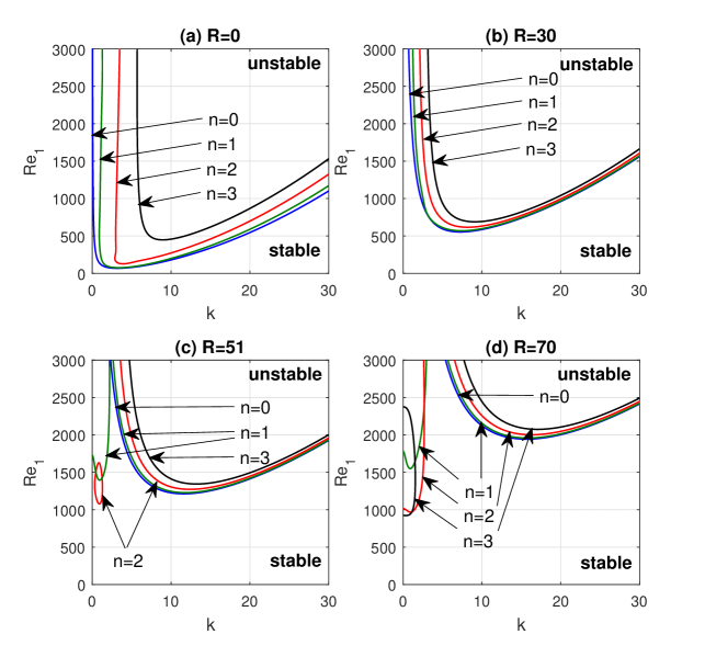
Figure 1: Neutral curves for the first 4 azimuthal modes ($n=0,\dots,3$), $a=2$ and $\mbox{{Re}}_{2}=0$: (a) - $R=0$; (b) - $R=30$; (c) - $R=50$; (d) - $R=70$.

The neutral curves for the classical Couette-Taylor flow ($R=0$) are shown in Fig. 1(a). When the azimuthal Reynolds number $\mbox{{Re}}_{1}$ increases from zero, the mode that becomes unstable first is an axisymmetric mode ($n=0$) for any value of the axial wave number $k\geq 0$. By minimizing $\mbox{{Re}}_{1}$ over all $n$ and $k$, we can obtain the critical Reynolds number $\mbox{{Re}}_{1cr}$ and the corresponding values of $n$ and $k$: $\mbox{{Re}}_{1cr}\approx 68.2$, $n_{cr}=0$ and $k_{cr}\approx 3.16$ in Fig. 1(a). Figure 1(b) displays the neutral curves for $R=30$. One can see that the curves keep qualitatively the same shape (as those in 1(a)), but are shifted upwards (to higher values of $\mbox{{Re}}_{1}$) and to the right (to the region of shorter axial waves). The critical values of $\mbox{{Re}}_{1}$, $n$ and $k$ in Fig. 1(b) are: $\mbox{{Re}}_{1cr}\approx 553.5$, $n_{cr}=0$ and $k_{cr}\approx 7.24$. As $R$, the Couette-Taylor modes shift further up and to the right. This however is not the end of the story. When the radial Reynolds number becomes sufficiently high, another neutral curve for the mode $n=1$ (disconnected from the corresponding Couette-Taylor mode) appears in the long wave region of the $(k,\mbox{{Re}}_{1})$ plane. This occurs at $R\approx 39.6834$. The new curve is closed and encircles a small oval instability region with a center approximately at $(k,\mbox{{Re}}_{1})=(0.84,1974)$. As $R$ increases further, the instability region for mode $n=1$ grows and becomes attached to the vertical axis ($k=0$). Then (at $R\approx 49.953$), another oval instability region for the mode $n=2$ appears. At first the instability regions for modes $n=2$ and $n=1$ do not intersect, but as $R$ increases, they grow in size and overlap. Figure 1(c) shows the neutral curves for $R=51$. One can see that, in addition to the unstable region bounded by the axisymmetric Couette-Taylor mode, there are two intersecting unstable regions for modes $n=1$ and $n=2$ corresponding to long axial waves. The first of these is pretty large and attached to the vertical axis ($k=0$), while the second is a relatively small oval region. This oval region will grow with $R$ and also become attached to the vertical axis at higher values of $R$. The most unstable mode (the critical mode) in Fig. 1(c) (obtained by minimizing $\mbox{{Re}}_{1}$) is the non-axisymmetic mode with $\mbox{{Re}}_{1cr}\approx 1077$, $n_{cr}=2$ and $k_{cr}\approx 0.91$. Neutral curves for $R=70$ are shown in Fig. 1(d). Now there are three non-axisymmetric modes ($n=1,2,3$) that are unstable to perturbations with sufficiently small $k$. The most unstable mode is $n_{cr}=3$, and the corresponding critical Reynolds number and the axial wave number are $\mbox{{Re}}_{1cr}\approx 923.2$ and $k_{cr}\approx 0.384$. For $R=70$, all modes with $n>3$ remain stable.

Two conclusions can be drawn from the above observations: (i) the diverging radial flow forces the classical Couette-Taylor modes to shift from the region of relatively low $\mbox{{Re}}_{1}$ to the region of higher $\mbox{{Re}}_{1}$ and higher axial wave numbers; (ii) new spiral long-wave unstable modes appear when the radial Reynolds number increases and those become more unstable than the axisymmetric Couette-Taylor mode. These non-axisymmetric modes are what is left of inviscid unstable modes (see [21, 23, 26]) after the viscous effects were switched on.

3.2 Critical curves for converging and diverging flows with non-rotating outer cylinder

By computing neutral curves and then the critical azimuthal Reynolds number, $\mbox{{Re}}_{1cr}$ and the corresponding wave numbers $n_{cr}$ and $k_{cr}$ for different values of the radial Reynolds number, we can obtain stability/instability regions in the $(R,\mbox{{Re}}_{1})$ plane, separated by critical curves: $\mbox{{Re}}_{1}=\mbox{{Re}}_{1cr}(R)$. These are shown in Fig. 2 for $a=2,4\ \hbox{and}\ 8$.

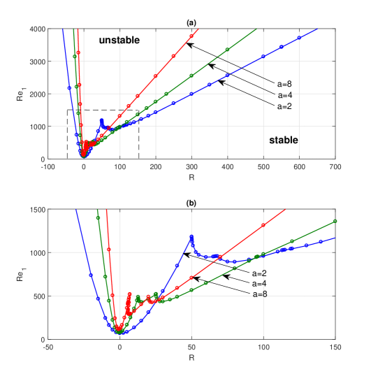
Figure 2: Critical curves for the diverging flow with the fixed outer cylinder ($\mbox{{Re}}_{2}=0$) for $a=2,4,\ \hbox{and}\ 8$. Circles show the computed points; solid curves are obtained by linear spline interpolation. Figure (b) is a magnified rectangular region (bounded by dashed lines) of figure (a).

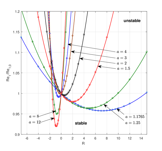
Figure 3: Critical values of $\mbox{{Re}}_{1}$ (normalized by $\mbox{{Re}}_{1,0}$, the critical value of $\mbox{{Re}}_{1}$ at $R=0$) for $-7<R<15$ and various values of $a$.

In Fig. 2, circles represent the computed points, and solid curves are obtained by linear spline interpolation. Figure 2(b) is obtained by enlarging the rectangular part of Fig. 2(a) (bounded by dashed lines). Nevertheless, there is a subtle effect which is not seen even in Figure 2(b): the global minimum of the critical curve for $a=2$ is attained not at $R=0$ but at $R\approx 0.56$ ($\mbox{{Re}}_{1}\approx 67.86$), so that a very weak diverging radial flow has a small destabilising effect. This agrees with what had been found earlier by Min & Lueptow [34] for $a$ in the range $[1.05,2]$ (see also [24]).

To better understand the dependence of the stability properties of the flow on the gap size, we have considered relatively weak radial flows ($|R|<15$) in more detail, paying particular attention to wider gaps ($a>2$). Critical curves for several values of $a$, normalized by $\mbox{{Re}}_{1,0}$, the critical value of $\mbox{{Re}}_{1}$ at $R=0$ (no radial flow), are shown in Fig. 3. Curves for $a\leq 2$ agree with the corresponding curves in [34, 24] (and this gives additional validation to our numerical computations). Figure 3 shows that the global minimum shifts to the left, when $a$ increases, and the minimum is attained at $R=0$ for $a\approx 2.64$ and at negative $R$ for wider gaps, $a>2.64$. This means that the effect of a weak radial flow for $a>2.64$ is opposite to that for $a<2.64$. In other words, a weak converging radial flow has a destabilizing effect, while a weak diverging flow is stabilising for $a>2.64$. This fact appears to have been missed in previous studies.

Now we return to the discussion of the global picture. Figure 2 shows that when the radial Reynolds number decreases from its value at the global minimum, the critical values of $\mbox{{Re}}_{1}$ monotonically increase for all values of $a$ considered in the present paper, and for sufficiently strong converging radial flows ($R<0$), the growth of the critical Reynolds number $\mbox{{Re}}_{1}$ becomes quite rapid as $R$ decreases. The critical mode remains axisymmetric and the critical axial wave number increases (the critical wave numbers, $n_{cr}$ and $k_{cr}$, as functions of $R$ are shown in Fig. 4(a,b)).

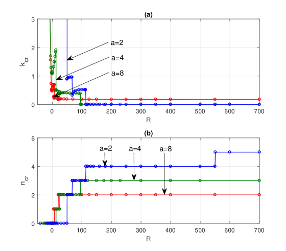
Figure 4: Critical values of azimuthal and axial wave numbers, $n_{cr}$ and $k_{cr}$. Circles show the computed points; solid curves are obtained by linear spline interpolation. Figure (a) shows $k_{cr}$ versus $R$ and figure (b) - $n_{cr}$ versus $R$.

When the radial Reynolds number increases from its value at the global minimum, the behaviour of the critical curves is more interesting. At first, over a finite interval (in $R$), the critical Reynolds number, $\mbox{{Re}}_{1cr}$, increases. Then, at a certain value of $R$, it starts decreasing, attains a local minimum and then increases over another finite interval up to another value of $R$, at which it starts decreasing again. Such behaviour may be repeated several times depending on the thickness of the gap. Each transition from growth to decay occurs at a point where the smoothness of the critical curve is lost (see Fig. 2) due to switching to a critical mode with different azimuthal and axial wave numbers.

Critical values of the axial and azimuthal wave numbers, $k_{cr}$ and $n_{cr}$, as functions of $R$ are shown in Fig. 4. The jumps in $k_{cr}$ occur when the azimuthal wave number, $n_{cr}$, of the most unstable mode changes. The number of transitions from one value of $n_{cr}$ to another depends on the gap between the cylinders: it is smaller for larger gaps. In all transitions in Fig. 4(b), $n_{cr}$ increases by $1$, except for the first transition for $a=2$ where the azimuthal wave number jumps from $n_{cr}=0$ to $n_{cr}=2$.

The above observations are in agreement with the results of Martinand et al [32] where the appearance of non-axisymmetric unstable modes have been found for $a=4$ (see Fig. 4 in [32]). For large $R$ ($R>600$ in Fig. 4), the critical azimuthal wave number remains unchanged, while the critical value of the axial wave number approaches a limit. Both the critical azimuthal wave number and the limit of the critical axial wave number coincide with values provided by the inviscid theory [23] (and this gives one more validation for our numerical results). For sufficiently large $R$, the most unstable modes are two-dimensional modes (i.e. $k_{cr}\to 0$ as $R\to\infty$) with $n_{cr}=5$ for $a=2$ and $n_{cr}=3$ for $a=4$, and this observation is consistent with the inviscid theory (see [23]). For $a=8$, the azimuthal wave number of the most unstable mode is $n_{cr}=2$, while the critical axial wave number does not vanish in the limit $R\to\infty$, rather, it tends to a finite limit: $k_{cr}\to 0.177$ as $R\to\infty$. This is also in agreement with the inviscid theory. Note that this fact has been missed in [23] where it was reported that the most unstable inviscid mode is two-dimensional for all $a$ ($a=2,4\ \hbox{and}\ 8$).

Another connection of the stability/instability regions in Fig. 2 with the inviscid theory is that, for large $R$, the slope of each curve tends to a limit determined by the inviscid theory, namely:

$$\frac{\mbox{{Re}}_{1cr}}{R}=(a-1)\,\gamma_{1}\ \to\ (a-1)\,\gamma_{div}(a)\quad\hbox{as}\quad R\to\infty$$

where $\gamma_{div}(a)$ is the critical value of $\gamma_{1}$ for the diverging flow in the inviscid theory (see [23]): $\gamma_{div}(2)\approx 5.73$, $\gamma_{div}(4)\approx 2.68$ and $\gamma_{div}(8)\approx 1.75$. Two more interesting features can be seen in Figs. 2 and 4: (i) the value of the radial Reynolds number, at which the first transition from an axisymmetric critical mode to a non-axisymmetric one occurs, is smaller for larger values of $a$ and (ii) for sufficiently large $R$, the azimuthal wave number of the most unstable mode is higher for smaller $a$. We note in passing that for larger values of $a$ (beyond $a=8$), the azimuthal wave number of the most unstable mode seems to remain unchanged: $n_{cr}=2$.

The main conclusions that can be drawn from Figs. 2, 3 and 4 are: (i) for $a>2.64$, i.e. for a large gap between the cylinders, a weak diverging flow has a stabilising effect on the Couette-Taylor flow, while a weak converging flow is destabilising, which is the opposite effect to what happens for relatively narrow gaps; (ii) the non-axisymmetric unstable modes, originated from the inviscid instability (see [21, 23, 26]), can be observed at moderate values of the radial Reynolds number: $R\gtrsim 50$ for $a=2$, $R\gtrsim 12.8$ for $a=4$ and $R\gtrsim 7$ for $a=8$.

3.3 Critical curves for converging and diverging flows when the outer cylinder is rotating

So far, we have looked at a particular class of the diverging and converging flows with fixed outer cylinder. Now we examine the effect of the rotation of the outer cylinder on the stability of the basic flow. To this end, we have computed the critical curves on the $(R,\mbox{{Re}}_{1})$ plane for several nonzero values of $\mbox{{Re}}_{2}$ for $a=4$. These are shown on Fig. 5.

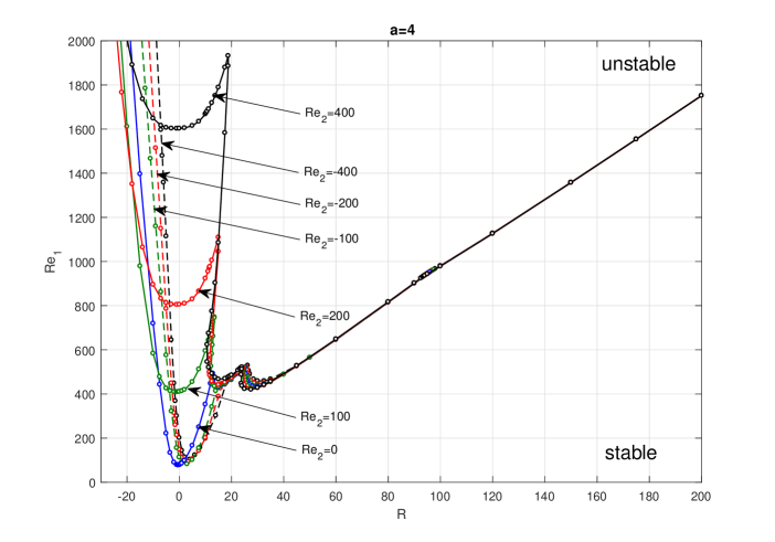
Figure 5: Critical curves for the converging and diverging flows for $a=4$ and $\mbox{{Re}}_{2}=-400,-200,-100,0,100,200,400$. Circles show the computed points; solid curves are obtained by linear spline interpolation.

Evidently, when the outer cylinder is rotating in the opposite direction relative to the inner one ($\mbox{{Re}}_{2}<0$), the critical curves slightly shift to the right, but their shape remains very similar to the curve for $\mbox{{Re}}_{2}=0$. When the cylinders are rotating in the same direction ($\mbox{{Re}}_{2}>0$), the part of the curve near the vertical line $R=0$ rapidly shifts up (with $\mbox{{Re}}_{2}$), because the classical Couette-Taylor flow (without the radial flow) becomes more stable. Interestingly, the part of the critical curve corresponding to the inviscid instability changes very little even for moderate positive values of $R$. For sufficiently large $R$ ($R>100$), the critical curves for $\mbox{{Re}}_{2}\in[-400,400]$ are almost indistinguishable. This means that the stability properties of the diverging flow are almost independent of whether or not the outer cylinder is rotating, and this is consistent with earlier results reported in [22].

The critical values of the axial and azimuthal wave numbers as functions of $R$ for $a=4$ and several fixed values of $\mbox{{Re}}_{2}$ are presented in Fig. 6. Figure 6(a) shows $k_{cr}$ versus $R$; the jumps in $k_{cr}$ correspond to transitions between modes with different azimuthal wave numbers (see Fig. 6(b)). The qualitative behaviour of the curves, $k_{cr}(R)$, remains very similar when $\mbox{{Re}}_{2}$ is varied in the interval $[-400,400]$; the curves for positive $\mbox{{Re}}_{2}$ shift slightly to the left, while those for negative $\mbox{{Re}}_{2}$ shift to the right. For all $\mbox{{Re}}_{2}\in[-400,400]$ and for sufficiently large positive $R$ ($R\geq 100$), the critical value of the axial wave number remains equal to zero, with the critical azimuthal wave number being equal to $3$. Thus, for sufficiently large positive $R$, the most unstable mode is two-dimensional ($k_{cr}=0$) with the azimuthal wave number $n_{cr}=3$, and this is in agreement with the inviscid theory [23].

The behaviour of the critical azimuthal wave number, $n_{cr}$, for several values of $\mbox{{Re}}_{2}$ is shown in Fig. 6(b). For $\mbox{{Re}}_{2}=-100,100,200$ and $400$, it is similar to that for $\mbox{{Re}}_{2}=0$. For $\mbox{{Re}}_{2}=-200$ and $-400$, $n_{cr}$ becomes nonzero for the converging flow ($R<0$). One can see in Fig. 6(b) that $n_{cr}$ may be equal to $1$ for $\mbox{{Re}}_{2}=-200$, and to $1$ and $2$ for $\mbox{{Re}}_{2}=-400$. This, however, is not very surprising because similar results are well-known for the classical Couette-Taylor flow (see e.g. [9]): the most unstable mode becomes non-axisymmetric when the cylinders rotate in opposite directions with sufficiently high angular velocities, i.e. for $\mbox{{Re}}_{2}<0$ and $|\mbox{{Re}}_{2}|\gg 1$. For $a=4$, the transition from $n_{cr}=0$ to $n_{cr}=1$ in the classical Couette-Taylor flow occurs at $\mbox{{Re}}_{2}\approx-1050$. Figure 6(b) shows the converging radial flow forces such transition at $\mbox{{Re}}_{2}$ as low as $200$.

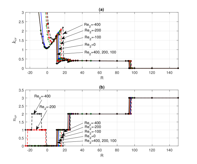
Figure 6: Critical values of the axial and azimuthal wave numbers, $k_{cr}$ and $n_{cr}$, versus $R$ for $a=4$ and $\mbox{{Re}}_{2}=-400,-200,-100,0,100,200,400$. Circles show the computed points; solid curves are obtained by linear spline interpolation.

3.4 Critical curves for converging flows with non-rotating inner cylinder

Now we consider the situation when the inner cylinder is fixed. It is well-known that the classical Couette-Taylor flow is stable in this case. If we impose a diverging radial flow ($R>0$), the basic flow remains stable. However, a converging radial flow can be destabilising. Figure 7(a) shows the stability/instability regions in the $(R,\mbox{{Re}}_{2})$ plane for $\mbox{{Re}}_{1}=0$ and $a=2,4\ \hbox{and}\ 8$. Azimuthal wave number of the most unstable mode is shown in Fig. 7(b). As before, the circles represent the computed points; the solid curves are obtained by linear spline interpolation. In all cases, the axial wave number of the most unstable mode is zero (i.e. the most unstable mode is a two-dimensional azimuthal wave).

Figure 7: Figure (a): Critical curves for the converging flow with the fixed inner cylinder ($\mbox{{Re}}_{1}=0$) for $a=2,4,\ \hbox{and}\ 8$. Circles show the computed points; solid curves are obtained by linear spline interpolation. Figure (b): critical azimuthal wave number, $n_{cr}$, versus radial Reynolds number, $R$.

The critical curves for $a=2$ and $a=4$ have points where the derivative along the curve is discontinuous (this is similar to what we had for the diverging flow in the preceding subsection). These points are where the azimuthal wave number of the most unstable mode changes. There are no such points on the critical curve for $a=8$: it turns out that $n_{cr}=1$ for all relevant values of $R$. For sufficiently strong converging flows ($R<0$ and $|R|\gg 1$), both the values of the critical azimuthal wave number and the slopes of the curves agree with the inviscid results of [23]. In particular,

$$\frac{\mbox{{Re}}_{2cr}}{R}=-\frac{a-1}{a}\,\gamma_{2}\ \to\ -\frac{a-1}{a}\,\gamma_{conv}(a)\quad\hbox{as}\quad R\to-\infty$$

where $\gamma_{conv}(a)$ is the critical value of $\gamma_{2}$ for the diverging flow in the inviscid theory (see [23]): $\gamma_{conv}(2)\approx 7.16$, $\gamma_{conv}(4)\approx 4.21$ and $\gamma_{conv}(8)\approx 3.15$.

The above observations can be summarised as follows: (i) the essentially inviscid instability (described, e.g., in [23]) occurs even in situations where the classical Couette-Taylor flow is stable; (ii) it can be observed at moderate values of the radial Reynolds number (though considerably higher than those for the diverging flow considered in section 3.2): $R\lesssim-105.485$ for $a=2$, $R\lesssim-80.98$ for $a=4$ and $R\lesssim-76.203$ for $a=8$.

3.5 Critical curves on the $(\mbox{{Re}}_{2},\mbox{{Re}}_{1})$ plane for diverging flows and weak converging flows

Now we consider critical curves on the $(\mbox{{Re}}_{2},\mbox{{Re}}_{1})$ plane. Since the stability properties of the basic flow do not change under simultaneous change of signs of the angular velocities of the cylinders, it is sufficient to consider only the half-plane $\mbox{{Re}}_{1}\geq 0$. The critical curves for several values of $R$, which correspond to diverging flows ($R>0$) and weak converging flows ($R<0$ and $|R|\leq 10$), are plotted in Figs. 8-10 (strong converging flows will be dealt with separately, in the next section; this is done for the sake of clarity of presentation, so that the figures are not overcrowded with curves). As before, circles represent the computed points, and solid curves are obtained by linear spline interpolation. For the classical Couette-Taylor flow, the critical curves separating stability/instability regions on the $(\mbox{{Re}}_{2},\mbox{{Re}}_{1})$ plane are well-known and agree with the experimental stability diagram of Andereck et al. [1] (see also [9]). The unstable region lies to the left of the Rayleigh line

$$\mbox{{Re}}_{1}=a\,\mbox{{Re}}_{2}$$

and the critical curve approaches the Rayleigh line asymptotically as $\mbox{{Re}}_{2}\to\infty$. It turns out that the presence of a diverging (or converging) radial flow considerably changes the picture of Andereck et al. [1].

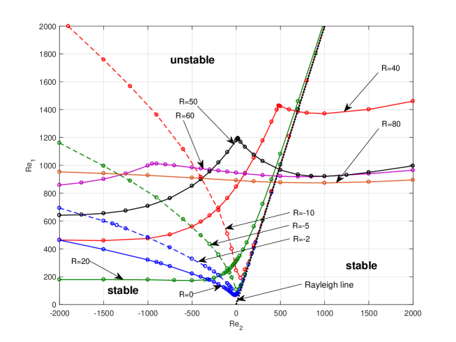
Figure 8: Critical curves on the $(\mbox{{Re}}_{2},\mbox{{Re}}_{1})$ plane for $a=2$ and several values of $R$.

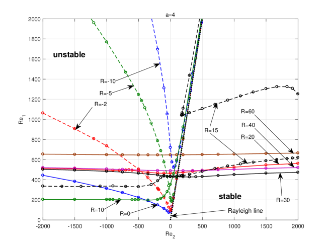
Figure 9: Critical curves on the $(\mbox{{Re}}_{2},\mbox{{Re}}_{1})$ plane for $a=4$ and several values of $R$.

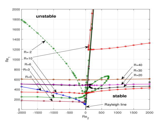
Figure 10: Critical curves on the $(\mbox{{Re}}_{2},\mbox{{Re}}_{1})$ plane for $a=8$ and several values of $R$.

Figure 8 shows the critical curves on the $(\mbox{{Re}}_{2},\mbox{{Re}}_{1})$ plane for $a=2$ and various values of the radial Reynolds number, $R$. A relatively weak converging radial flow ($R<0$) does not considerably change the critical curves for positive $\mbox{{Re}}_{2}$, but, for $\mbox{{Re}}_{2}<0$ (counter-rotating cylinders), it notably shifts the critical curve up (towards higher values of $\mbox{{Re}}_{1}$). As the converging radial flow becomes stronger (equivalently, as $|R|$ increases), the left part of the critical curve moves further up, so that the instability region rapidly shrinks, while the part of the critical curve near the Rayleigh line remains almost unchanged and lies to the left of the Rayleigh line for all negative values of $R$ shown in Fig. 8. At the same time, the minimum point of the curve, situated near the vertical axis ($\mbox{{Re}}_{2}=0$), moves up each time when we increase $|R|$. Eventually (for $|R|\gtrsim 50$), the instability region completely disappears from Fig. 8 (moves up beyond the frame of the figure). So, the converging flow seems to produce a strong stabilising effect (and this agrees with the earlier results of [34, 24]).

The situation is quite different when a diverging radial flow is imposed. At first, when the radial flow is relatively weak, the only change is that the part of the critical curve corresponding to negative $\mbox{{Re}}_{2}$ is shifted down (see the critical curve for $R=20$ in Fig. 8). The other part of the curve remains very close to that for the classical Couette-Taylor flow. As the radial Reynolds number increases further, there comes a point at which the picture radically changes. The critical curve for $R=40$ in Fig. 8 crosses the Rayleigh line, so that the instability region extends to the right of the Rayleigh line where the Rayleigh stability criterion would predict stability. The reason for such behaviour is the same as in section 3.2: it is a result of the inviscid instability (see [21, 23, 26]), and the point of non-smoothness of the critical curve (at $\mbox{{Re}}_{2}\approx 490$) is where the spiral wave inherited from the inviscid instability becomes more unstable than the axisymmetric Taylor mode. An increase in $R$ to $R=50$ results in shrinking of the instability region to the left of the Rayleigh line and its extension to the right of the Rayleigh line. Further increases in $R$ make the critical curves flatter. For example, the curve for $R=80$ looks almost like a horizontal straight line. This means that for sufficiently high radial Reynolds numbers, the stability properties of the basic flow are almost independent of $\mbox{{Re}}_{2}$, i.e. the effect of the outer cylinder becomes very weak, which is in agreement with earlier results [22].

Critical curves for $a=4$ and $a=8$ shown in Figs. 9 and 10 look similar to the curves in Fig. 8. There are a couple of important differences though. First, the inviscid instability emerges at lower radial Reynolds numbers: this happens for $R\gtrsim 15$ for $a=4$ (Fig. 9) and for $R\gtrsim 6$ for $a=8$ (Fig. 10). Second, when the instability region crosses Rayleigh line, it covers a tongue-like area to the right of it (see the critical curve for $R=6$ in Fig. 10). It grows when $R$ increases (see the curves for $R=10$ in Fig. 10 and for $R=15$ in Fig. 9), and its upper and right boundaries very quickly move beyond the upper and right edges of Figs. 9 and 10 ($R\gtrsim 20$ in Fig. 9 and $R\gtrsim 15$ in Fig. 10). Again, for sufficiently high $R$, the critical curves look like horizontal straight lines.

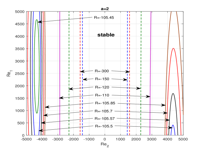
Figure 11: Stability/instability regions on the $(\mbox{{Re}}_{2},\mbox{{Re}}_{1})$ plane for $a=2$ and several negative values of $R$.

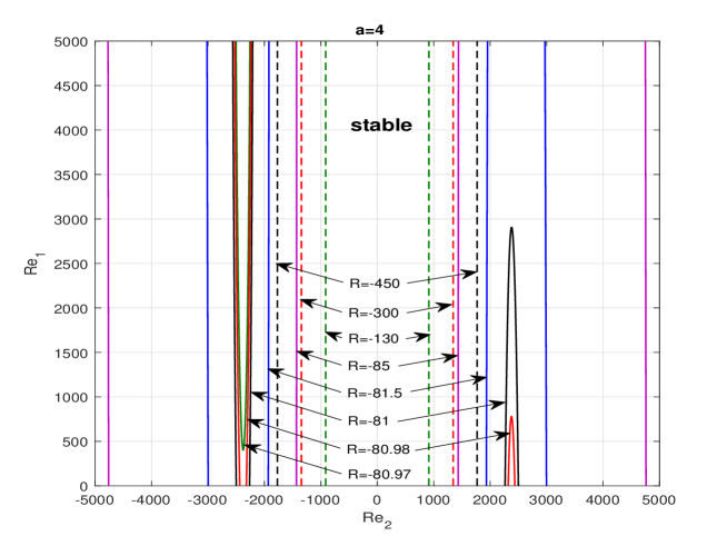
Figure 12: Stability/instability regions on the $(\mbox{{Re}}_{2},\mbox{{Re}}_{1})$ plane for $a=4$ and several negative values of $R$.

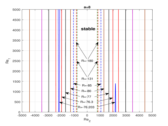
Figure 13: Stability/instability regions on the $(\mbox{{Re}}_{2},\mbox{{Re}}_{1})$ plane for $a=8$ and several negative values of $R$.

It is evident from Figs. 8-10 that for the cylinders rotating in opposite directions ($\mbox{{Re}}_{2}<0$), a weak diverging radial flow is destabilizing: the critical curves for (relatively) small positive $R$ are below the curve for the classical Couette-Taylor flow provided that the magnitude of $\mbox{{Re}}_{2}$ is sufficiently large ($\mbox{{Re}}_{2}\lesssim-100$). Figures 8-10 also show a sufficiently strong diverging flow has stabilizing effect. Therefore, there must be an optimal value of $R$ corresponding to the lowest critical value of $\mbox{{Re}}_{1}$ for each value of $\mbox{{Re}}_{2}<0$. We have computed $\mbox{{Re}}_{1*}=\mbox{{Re}}_{1cr}(R_{*})=\min_{R\geq 0}\mbox{{Re}}_{1cr}(R)$ for several values of $\mbox{{Re}}_{2}$ for $a=4$, as well as the difference, $\Delta\mbox{{Re}}_{1}$, between the critical value of $\mbox{{Re}}_{1}$ for the classical Couette-Taylor flow, $\mbox{{Re}}_{1,0}$, and $\mbox{{Re}}_{1*}$ (i.e. $\Delta\mbox{{Re}}_{1}$ defined as $\Delta\mbox{{Re}}_{1}=\mbox{{Re}}_{1,0}-\mbox{{Re}}_{1*}\,$). The results are shown in Table 1.

$\mbox{{Re}}_{2}$	-100	-200	-400	-600	-800	-1000	-1400
$R_{*}$	2.47	2.89	3.48	3.82	4.04	4.20	4.52
$\mbox{{Re}}_{1*}$	81.6	91.8	102	108	113	117	122
$\Delta\mbox{{Re}}_{1}$	31.6	56.9	99.5	135	167	196	247

Table 1: Values of $R_{*}$, $\mbox{{Re}}_{1*}$ and $\Delta\mbox{{Re}}_{1}$ for several negative values of $\mbox{{Re}}_{2}$ for $a=4$.

Evidently, the minimal critical value of $\mbox{{Re}}_{1}$, the optimal value of $R$ and the difference, $\Delta\mbox{{Re}}_{1}$, all grow when $\mbox{{Re}}_{2}$ decreases. However, the growth in $R_{*}$ and $\mbox{{Re}}_{1*}$ is pretty slow, while the gap between $\mbox{{Re}}_{1*}$ and the critical $\mbox{{Re}}_{1}$ for the classical Couette-Taylor flow widens much faster (it increases by a factor of $7.8$ as $\mbox{{Re}}_{2}$ varies from $-100$ to $-1400$. So, the destabilizing effect of the weak diverging radial flow is pretty strong and it becomes much stronger when $\mbox{{Re}}_{2}$ decreases.

3.6 Critical curves on the $(\mbox{{Re}}_{2},\mbox{{Re}}_{1})$ plane for strong converging flows

One of the findings of the preceding section is the stabilizing effect of the converging radial flow: the instability domain on the $(\mbox{{Re}}_{2},\mbox{{Re}}_{1})$ plane rapidly shrinks when $R$ decreases from $0$. However, we also saw in section 3.4 that the flow with a fixed inner cylinder ($\mbox{{Re}}_{1}=0$) becomes unstable for a sufficiently strong converging radial flow due to the inviscid instability [21]. So, unstable regions should also appear on the $(\mbox{{Re}}_{2},\mbox{{Re}}_{1})$ plane provided that $R<0$ and $|R|$ is sufficiently high. The results of calculations are presented in Figs. 11-13. Figure 11 shows the instability regions for $a=2$. When the converging flow is sufficiently strong ($R\approx-105.422$), a vertically elongated oval instability region, which is at first very small, appears in the second quadrant of the plane. As $R$ decreases, this oval region rapidly grows. The instability region for $R=-105.45$ is shown in Fig. 11. As $R$ decreases further, the upper and lower parts of the oval instability region move beyond the edges of the figure (see the curve for $R=-105.5$ in Fig. 11). At the same time the upper part of another oval instability region emerges in the first quadrant. (It should be noted here that the picture on the upper half-plane can be continued to the lower half-plane using the central symmetry with respect to the origin. This means that two oval regions appear simultaneously in the second and forth quadrants of the whole $(\mbox{{Re}}_{2},\mbox{{Re}}_{1})$ plane and then grow in size penetrating into the first and third quadrants when $R$ decreases.) As the strength of the converging flow increases further, the ovals continue to grow in size and their centers slowly drift away from the vertical axis ($\mbox{{Re}}_{2}=0$). As a result the region of stability near the vertical axis, while shrinking at first, never completely disappears, and starts growing in width at $R\approx-170$. For all curves in Fig. 11, the critical modes are two-dimensional ($k_{cr}=0$). On each curve, the critical azimuthal wave number does not change (so that the critical curves appear to be smooth), and $n_{cr}=2$ for all curves except for $R=-300$, for which $n_{cr}=3$. Critical curves for $a=4$ and $a=8$ are presented in Figs. 12 and 13. They look similar to those in Fig. 11. For all critical curves in Figs. 12 and 13, $k_{cr}=0$. In Fig. 12, $n_{cr}=1$ for all $R$ except $R=-300$ and $R=-450$, for which $n_{cr}=2$. In Fig. 13, $n_{cr}=1$ for all curves. It is evident from Figs. 12 and 13 that, compared with the case of $a=2$, the instability occurs for slightly weaker radial flows (at $R\approx-80.97$ for $a=4$ and $R\approx-70.203$ for $a=8$) and that the oval instability regions become more elongated for larger $a$ and lie closer to the vertical axis $\mbox{{Re}}_{2}=0$. These observations lead us to a conclusion that, although the effect of a weak converging flows is stabilising, it becomes destabilising provided that the converging radial flow is sufficiently strong.

4 Discussion

We have investigated the linear stability of steady viscous incompressible flows between rotating porous cylinders with a radial flow for a wide range of the key parameters of the flow: the ratio of the radii of the cylinders, $a$, the radial Reynolds number, $R$, and the inner and outer azimuthal Reynolds numbers, $\mbox{{Re}}_{1}$ and $\mbox{{Re}}_{2}$. This resulted in a detailed picture of the effect of a radial flow. In particular, we have obtained critical curves on the $(\mbox{{Re}}_{2},\mbox{{Re}}_{1})$ plane for $a=2,4,\ \hbox{and}\ 8$ and various values of $R$. These critical curves show that a relatively weak diverging radial flow ($R>0$) can have both stabilising and destabilising effects depending on $\mbox{{Re}}_{2}$. The critical curves for $R=20$ in Fig. 8, for $R=10$ in Fig. 9 and for $R=3$ in 10 show that for negative $\mbox{{Re}}_{2}$ (counter-rotating cylinders), the basic flow is more stable (than the classical Couette-Taylor flow) for small to moderate negative $\mbox{{Re}}_{2}$, but it becomes more unstable for large negative $\mbox{{Re}}_{2}$; for positive $\mbox{{Re}}_{2}$ (co-rotating cylinders), the critical curves remain close to the classical Couette-Taylor curves. As the radial Reynolds number increases, the critical modes take the form of spiral or planar azimuthal waves rather than the classical Taylor vortices. These waves are what is left of the inviscid instability (studied earlier in [21, 26, 23]) when the viscosity is taken into account. The key consequence of this inviscid instability is that some flows in the region to the right of the Rayleigh line (which are stable in the classical Couette-Taylor flow) become unstable if a sufficiently strong diverging radial flow is present. The most interesting (and unexpected) result here is that the inviscid instability survives for radial Reynolds numbers as low as $R=40$ for $a=2$ (see Fig. 8), $R=15$ for $a=4$ (see Fig. 9) and $R=6$ for $a=8$ (see Fig. 10). This makes an experimental observation of the inviscid instability feasible.

In the case of converging radial flow(see Figs. 7, 11-13), the inviscid instability again invades the regions where the classical Couette-Taylor flow is stable (this occurs, e.g., when the inner cylinder is not rotating). However, the converging radial flow has to be rather strong to produce the instability. We found that it can be observed at $R\lesssim-105.45$ for $a=2$ (Fig. 11), $R\lesssim-80.97$ for $a=4$ (Fig. 12) and $R\lesssim-76.203$ for $a=8$ (Fig. 13). The absolute values of these numbers are considerably higher than their counterparts for the diverging flows, but still moderate, so that the inviscid instability in converging flows can, hopefully, be observed in experiments.

Within the range of parameters considered in this paper, the picture of linear instabilities that emerges from Figs. 8-13 is complete in the sense that there are no other linear instabilities. However, as was discussed in [22], the viscous boundary layers that appear near the outflow part of the boundary can also be unstable. In particular, it has been shown there that, at high radial Reynolds numbers, this instability of the boundary layer is equivalent to the instability of the asymptotic suction profile (see, e.g., [19, 18, 10]). This viscous boundary layer instability is, however, well separated from all the instabilities discussed in the present paper: the former requires very large values of $|\gamma_{1}-\gamma_{2}|$ ($|\gamma_{1}-\gamma_{2}|>5\cdot 10^{4}$), while the latter occur at moderate values of $\gamma_{1}$ and $\gamma_{2}$.

There are still quite a few open problems in this area. For example, it would be interesting to develop a weakly nonlinear theory of the oscillatory ‘inviscid’ instabilities considered in the present paper. The recent theory of Martinand et al [32] (where the effects of both radial and axial flows were considered) is not directly applicable to the case without axial flow. This is because the axial flow breaks the mirror symmetry of the problem, so that the eigenvalues associated with neutral modes are simple, while they are double when there is no axial flow. The weakly nonlinear analysis taking into account this multiplicity and the symmetry breaking by a weak axial flow is a topic of a continuing investigation. Another interesting question is whether the instabilities discussed here have any relevance to accretion disks in astrophysics. The weakly compressible analysis of Kerswell [26] is not sufficient (as was pointed out by Kerswell himself) because the azimuthal velocity in thin accretion disks is believed to be highly supersonic (see, e.g., [12]). This is also a problem for a future investigation.

References

- Andereck et al. [1986] Andereck, C.D., Liu, S.S. & Swinney, H.L. 1986 Flow regimes in a circular Couette system with independently rotating cylinders. J. Fluid Mech. 164, 155–183.
- Antontsev et al. [1990] Antontsev, S. N., Kazhikhov, A. V. & Monakhov, V. N. 1990 Boundary value problems in mechanics of nonhomogeneous fluids [translated from the Russian]. Studies in Mathematics and its Applications, Vol. 22, North-Holland Publishing Co., Amsterdam, 309 pp.
- Bahl [1970] Bahl, S. K. 1970 Stability of viscous flow between two concentric rotating porous cylinders. Def. Sci. J. 20(3), 89–96.
- Beadoin & Jaffrin [1989] Beadoin, G. & Jaffrin, M. Y. 1989 Plasma filtration in Couette flow membrane devices. Artif. Organs 13(1), 43–51.
- Beavers & Joseph [1967] Beavers, G. S. & Joseph, D. D. 1967 Boundary conditions at a naturally permeable wall. J. Fluid Mech. 30(1), 197–207.
- Billant & Gallaire [2005] Billant, P. & Gallaire, F. 2005 Generalized Rayleigh criterion for non-axisymmetric centrifugal instabilities. J. Fluid Mech. 542, 365–379.
- Chandrasekhar [1961] Chandrasekhar, S. 1961 Hydrodynamic and hydromagnetic stability. Clarendon Press, Oxford, 652 pp.
- Chang & Sartory [1967] Chang, S. & Sartory, W. K. 1967 Hydromagnetic stability of dissipative flow between rotating permeable cylinders. J. Fluid Mech. 27, 65–79.
- Chossat & Iooss [1994] Chossat, P. & Iooss, G. 1994 The Couette-Taylor Problem. Applied Mathematical Sciences., Vol. 102. Springer, New York, 233 pp.
- Doering et al. [2000] Doering, C. R., Spiegel, E. A. & Worthing, R. A. 2000 Energy dissipation in a shear layer with suction. Phys. Fluids 12(8), 1955–1968.
- Drazin & Reid [1981] Drazin, P. G. & Reid, W. H. 1981 Hydrodynamic stability. Cambridge University Press.
- Frank et al. [2002] Frank, J., King A. & Raine, D. 2002 Accretion Power in Astrophysics. Cambridge University Press, 3rd Edition.
- Fujita et al. [1997] Fujita, H., Morimoto, H. & Okamoto, H. 1997 Stability analysis of Navier–Stokes flows in annuli. Mathematical methods in the applied sciences 20(11), 959–978.
- Furth et al. [1963] Furth, H. P., Killeen, J. and Rosenbluth, M. N. 1963 Finite resistivity instabilities of a sheet pinch. Phys. Fluids 6(4) (1963) 459–484.
- Gallet et al. [2010] Gallet, B., Doering, C. R. & Spiegel, E. A. 2010 Destabilizing Taylor-Couette flow with suction. Phys. Fluids 22(3), 034105.
- Gellert & Rüdiger [2009] Gellert, M. & Rüdiger, G. 2000 Stratorotational instability in Taylor–Couette flow heated from above. J. Fluid Mech. 12(8), 1955–1968.
- Giordano et al [1998] Giordano, R. C., Giordano, R. L. C., Prazerest,D. M. F. and Cooney, C. L. 1998 Analysis of a Taylor–Poiseuille vortex flow reactor–I: Flow patterns and mass transfer characteristics. Chemical Engineering Science 53(20), 3635–3652.
- Hocking [1975] Hocking, L. M. 1975 Non-linear instability of the asymptotic suction velocity profile. Quarterly Journal of Mechanics and Applied Mathematics 28(3), 341–353.
- Hughes & Reid [1965] Hughes, T. H. & Reid, W. H. 1965 On the stability of the asymptotic suction boundary-layer profile. J. Fluid Mech. 23(4), 715–735.
- Ilin [2008] Ilin, K. 2008 Viscous boundary layers in flows through a domain with permeable boundary. Eur. J. Mech. B/Fluids. 27, 514–538.
- Ilin & Morgulis [2013] Ilin, K. & Morgulis, A. 2013 Instability of an inviscid flow between porous cylinders with radial flow. J. Fluid Mech. 730, 364–378.
- Ilin & Morgulis [2015] Ilin, K. & Morgulis, A. 2015 Instability of a two-dimensional viscous flow in an annulus with permeable walls to two-dimensional perturbations. Phys. Fluids 27, 044107.
- Ilin & Morgulis [2017] Ilin, K. & Morgulis, A. 2017 Inviscid instability of an incompressible flow between rotating porous cylinders to three-dimensional perturbations. Eur. J. Mech. - B/Fluids 62(1), 46–60.
- Johnson & Lueptow [1997] Johnson, E. C. & Lueptow, R. M. 1997 Hydrodynamic stability of flow between rotating porous cylinders with radial and axial flow. Phys. Fluids 9(12), 3687–3696.
- Kersale et al. [2004] Kersale, E., Hughes, D. W., Ogilvie, G. I., Tobias, S. M. & Weiss, N. O. 2004 Global magnetorotational instability with inflow. I. Linear theory and the role of boundary conditions. Astrophys. J. 602(2), 892–903.
- Kerswell [2015] Kerswell, R. R. 2015 Instability driven by boundary inflow across shear: a way to circumvent Rayleigh’s stability criterion in accretion disks? J. Fluid Mech. 784, 619–663.
- Kolesov & Shapakidze [1999] Kolesov, V. & Shapakidze, L. 1999 On oscillatory modes in viscous incompressible liquid flows between two counter-rotating permeable cylinders. In: Trends in Applications of Mathematics to Mechanics (ed. G. Iooss, O. Gues & A Nouri), Chapman and Hall/CRC, pp. 221–227.
- Kolyshkin & Vaillancourt [1997] Kolyshkin, A. A. & Vaillancourt, R. 1997 Convective instability boundary of Couette flow between rotating porous cylinders with axial and radial flows. Phys. Fluids 9, 910–918.
- Korobkov et al [2014] Korobkov, M. V., Pileckas, K., Pukhnachov, V. V. & Russo, R. 2014 The flux problem for the Navier-Stokes equations. Russian Mathematical Surveys 69(6), 1065–1122 (translated from Uspekhi Mat. Nauk 69(6) (2014) 115–176).
- Leclercq et al. [2016] Leclercq, C., Nguyen, F. & Kerswell, R. R. 2016 Connections between centrifugal, stratorotational and radiative instabilities in viscous Taylor–Couette flow. Phys. Rev. E 94, 043103.
- Martinand et al. [2009] Martinand, D., Serre, E. & Lueptow, R. M. 2009 Absolute and convective instability of cylindrical Couette flow with axial and radial flows. Phys. Fluids 21(10), 104102.
- Martinand et al [2017] Martinand, D., Serre, E. & Lueptow, R. M. 2017 Linear and weakly nonlinear stability analyses of cylindrical Couette flow with axial and radial flows. J. Fluid Mech. 824, 438–476.
- Meseguer & Trefethen [2003] Meseguer, A. & Trefethen, L.N. 2003 Linearized pipe flow to Reynolds number . Journal of Computational Physics 186(1), 178-197.
- Min & Lueptow [1994] Min, K. & Lueptow, R. M. 1994 Hydrodynamic stability of viscous flow between rotating porous cylinders with radial flow. Phys. Fluids 6(1), 144–151.
- Morgulis & Yudovich [2002] Morgulis, A. B. & Yudovich, V. I. 2002 Arnold’s method for asymptotic stability of steady inviscid incompressible flow through a fixed domain with permeable boundary. Chaos 12, 356–371.
- Press et al. [1992] Press, W. H., Teukolsky, S. A., Vetterling, W. T. & Flannery, B. P. 1992 Numerical recipes in Fortran 77: the art of scientific computing. Cambridge University Press.
- Serre et al. [2008] Serre, E., Sprague, M. A. & Lueptow, R. M. 2008 Stability of Taylor-Couette flow in a finite-length cavity with radial throughflow. Phys. Fluids 20(3), 034106.
- Temam & Wang [2000] Temam, R. & Wang, X. 2000 Remarks on the Prandtl equation for a permeable wall. Z. Angew. Math. Mech. 80, 835–843.
- Wroński et al. [1989] Wroński, S., Molga, E. & Rudniak, L. 1989 Dynamic filtration in biotechnology. Bioprocess Engineering 4(3), 99–104.
- Yudovich [2001] Yudovich, V. I. 2001 Rotationally symmetric flows of incompressible fluid through an annulus. Parts 1 and 2. Preprints VINITI no. 1862-B01 and 1843-B01 (in Russian).