Vector partition functions and Kronecker coefficients

Abstract

The Kronecker coefficients are the structure constants for the restriction of irreducible representations of the general linear group $GL(nm)$ into irreducibles for the subgroup $GL(n)\times GL(m)$. In this work we study the quasipolynomial nature of the Kronecker function using elementary tools from polyhedral geometry. We write the Kronecker function in terms of coefficients of a vector partition function. This allows us to define a new family of coefficients, the atomic Kronecker coefficients. Our derivation is explicit and self-contained, and gives a new exact formula and an upper bound for the Kronecker coefficients in the first nontrivial case.
Keywords: Kronecker products, rational polytopes, vector partition functions 2010 Subject classification: 05E10, 05E05, 17B10

1 Introduction

The subgroup restriction or branching problem investigates how an irreducible representation of a group $G$ decomposes into irreducibles when restricted to a subgroup $H.$ In this article, we study this branching for $GL(n)\times GL(m)$ viewed as a subgroup of $GL(nm)$ via the tensor product of matrices. The Kronecker coefficients are the structure constants for this branching. They are also important from a physicist’s point of view. Christandl, Harrow and Graeme have shown the relevance of Kronecker coefficients in the study of the spectra of bipartite quantum states with two fixed marginal states, and studied the implications of their findings in quantum information theory, [CHM07, CG06, Chr06, CDW12]. The restriction of $GL(4)$ to $GL(2)\times GL(2)$ is of interest in nuclear physics where it is called Wigner supermultiplet theory, [W37].

Irreducible representations of $GL(n)$ are indexed by partitions of length at most $n$. Therefore, the Kronecker coefficients are indexed by triples of partitions of the same weight, and bounded lengths. We denote by $g_{\mu,\nu,\lambda}$ the Kronecker coefficient indexed by $\mu,\nu,\lambda.$ Alternatively, the Kronecker coefficients $g_{\mu,\nu,\lambda}$ can be defined by the expression:

$$s_{\lambda}[XY]=s_{\lambda}(x_{1}y_{1},x_{1}y_{2}\cdots,x_{n}y_{m})=\sum_{\mu,\nu}g_{\mu,\nu,\lambda}\,s_{\mu}[X]s_{\nu}[Y]$$ (1)

where all partitions appearing in the equation have the same weight, and lengths bounded by $n,m$ and $nm$ respectively, and the $s_{\lambda}$’s denote the Schur polynomials.

The Kronecker function $\kappa_{m,n,l}$ is a function defined on triples of partitions $(\mu,\nu,\lambda)$ of lengths bounded by $n,m$ and $l$ respectively, by

$$\kappa_{n,m,l}(\mu,\nu,\lambda)=\kappa_{n,m,l}(\mu_{1},\ldots,\mu_{n},\nu_{1},\ldots,\nu_{m},\lambda_{1},\ldots,\lambda_{l}):=g_{\mu,\nu,\lambda}.$$ (2)

In this work, we use the restriction of the $Gl(nm)$-irreducible indexed by $\lambda$ to the subgroup $Gl(n)\times Gl(m)$ described by Eqn. (1) to compute of $\kappa_{n,m,l}$. We introduce a new family of coefficients (also indexed by triples of partitions) that we call the atomic Kronecker coefficients. They are defined by a single vector partition function. As a result, they count integer points in polytopes, satisfy the saturation hypothesis [Kir04, BOR09b], and are described by a piecewise quasipolynomial. We then show how to compute the actual Kronecker coefficients from these atomic coefficients. We also show that, for partitions of lengths $2$, $2$ and $4$, the atomic Kronecker coefficients are an upper bound for the Kronecker coefficients.

The atomic Kronecker coefficients share many properties with the reduced Kronecker coefficients (a family of coefficients lying between the Littlewood-Richardson coefficients and the Kronecker coefficients, defined in Section 3.8): They contain enough information to compute from them the value of any Kronecker coefficient as an alternating sum. Sometimes, the atomic Kronecker coefficients coincide with the Kronecker coefficients. However, the atomic Kronecker coefficients have a major advantage over the reduced Kronecker coefficients (that they share with the Littlewood–Richardson coefficients): They satisfy the saturation hypothesis, whereas the reduced Kronecker coefficients do not [PP20].

In this paper we provide the theory and framework for computing $\kappa_{n,m,nm}$, although we focus mainly on the Kronecker function $\kappa_{2,2,4}$. In subsequent work (with Stefan Trandafir) we will report on an explicit implementation of the techniques developed in this paper to compute the Kronecker function $\kappa_{2,3,6}$.

The structure of the paper is the following. We begin in Section 2 with a basic survey on polytopes and quasipolynomials. This is sufficient to understand the mechanics of our strategy. Our key idea is to use Eqn. (1) in conjunction with Cauchy’s definition for Schur functions as a quotient of alternants (equivalently, the Weyl character formula for the root system $A_{n}$) to make explicit the relation between Kronecker coefficients and points in a polytope.

In Section 3, we study the smallest nontrivial example, in which two of the partitions have length $\leq 2$. We provide concrete visualizations of the Kronecker functions $\kappa_{2,2,2}$ and $\kappa_{2,2,4}$. This can be made really explicit because the corresponding polyhedra are of dimension 1 and 2 respectively. We give a new explicit closed form (Theorem 7) for the Kronecker coefficients in terms of coefficients of a vector partition function $F_{2,2},$ as well as in terms of vector partition functions. Our formula identifies 7 terms (out of a possible total of 24) in the numerator of the Weyl character formula for the Weyl group $\mathbb{S}_{4}$, as the only terms contributing to the Kronecker coefficient. The number of chambers is large, even in the case 2-2-4, where it was determined to be 74 in [BOR09b, BOR09a]. We show that, in the case of Kronecker coefficients indexed by triples of partitions of length at most 2, 2, and 4, the atomic Kronecker coefficients give an upper bound for the value of the Kronecker coefficients (Theorem 17). We study the relative positions of the nonzero Littlewood–Richardson coefficients, reduced Kronecker coefficients, and atomic Kronecker coefficients inside the Kronecker cone (the polyhedral cone generated by the nonzero Kronecker coefficients). We study the dilated Kronecker coefficients, $g_{k\lambda,k\mu,k\nu}$, defined for fixed $\lambda,\mu,$ and $\nu$, and $k\in\mathbb{N}$. We express these as a subseries of vector partition generating functions which implies that these are given by quasipolynomials in $k$. We show how to use Theorem 7 to compute the dilated Kronecker coefficients $g_{k\mu,k\nu,k\lambda}$ in the 2-2-4 case.

In Section 4 we consider the general situation. Theorem 26 presents an elementary but nontrivial change of variables which converts the quotient of alternants into a form recognizable as a vector partition function, which we call $F_{n,m}$. This facilitates our analysis since it returns us to the realm of Taylor series. The function $F_{n,m}$ is the generating function of the atomic Kronecker coefficients.

The piecewise quasipolynomial nature of the Kronecker function has been the focus of much interest. The piecewise quasipolynomiality follows from the work of Meinrenken and Sjamaar [MS99]. Both Christandl, Doran, and Walter [CDW12] and Baldoni, Vergne, and Walter [BVW16] describe and implement algorithms to compute the Kronecker coefficients. Pak and Panova obtained an interesting upper bound for the complexity of the calculation of the Kronecker coefficients, see the proof of Lemma 5.4 in [PP17b].

2 Polytopes and Quasipolynomials

This section is a primer on polytope point enumeration and quasipolynomiality. It can be skipped by those familiar with the topic. However, the examples we have chosen for this section are directly relevant in our study of the Kronecker coefficients.

A polyhedron $\mathcal{P}$ is the set of solutions of a (finite) system and inequalities:

$$\mathcal{P}=\{{\mathbf{x}}\in\mathbb{R}^{d}:A{\mathbf{x}}\leq{\mathbf{b}}\},$$

for a fixed matrix $A$ and vector ${\mathbf{b}}$, where the “$\leq$” sign is to be understood componentwise. A polyhedron is said to be rational if both $A$ and ${\mathbf{b}}$ have integer entries. A polytope is a bounded polyhedron. Note that any dilation of a polytope contains only a finite number of integer points.

The dimension of a polytope is the dimension of the affine space spanned by its vertices. A $k$-simplex is a $k$-dimensional polytope which is the convex hull of $k+1$ vertices.

A function $\phi:\mathbb{N}\to\mathbb{Q}$ is a (one-variable) quasipolynomial if there exist polynomials $p_{0},p_{1},\ldots,p_{k-1}$ in $\mathbb{Q}[t]$ and a natural number $m>0$, a period of $\phi$, such that

$$\phi(t)=p_{i}(t),\text{ for }t\equiv i\mod m.$$

The polynomials $p_{i}$ are the constituents of $\phi$. The degree of a quasipolynomial is the maximum of the degrees of its components.

Example 1.

Let $\mathcal{P}$ be the one-dimensional polytope $[0,1/2]$, and consider its integer dilations $k\mathcal{P}=[0,k/2]$, as illustrated in Figure 1. We want to count the number of integer points in the dilation of $\mathcal{P}$:

$$\phi_{\mathcal{P}}(k):=|\mathbb{Z}\cap k\mathcal{P}|$$

Equivalently, we are interested in counting the number of nonnegative integer solutions to the inequality $0\leq s_{1}\leq k/2$. Then

$$\phi_{\mathcal{P}}(k)=\left\lfloor\frac{k}{2}\right\rfloor+1=\begin{cases}\frac{k+2}{2}&\text{ if }k\equiv 0\mod 2\\ \frac{k+1}{2}&\text{ if }k\equiv 1\mod 2\end{cases}$$

is a linear quasipolynomial of period 2.

Figure 1: The one dimensional polytope $\mathcal{P}=[0,1/2]$ and its first four integer dilations. The volume of the $k$-th dilation is $\left\lfloor\frac{k}{2}\right\rfloor+1$, a quasipolynomial in $k$.

A vector partition of ${\mathbf{b}}\in\mathbb{N}^{d}$ is a way of decomposing ${\mathbf{b}}$ as a sum of nonzero vectors in $\mathbb{N}^{d}$. The order of the summands is irrelevant. We are interested in partitions whose parts (nonzero summands) belong to a fixed finite sub-multiset $S$ of $\mathbb{N}^{d}$. The vector partition function $p_{S}:\mathbb{N}^{d}\to\mathbb{N}$ is the function that evaluated at ${\mathbf{b}}$ gives the number of vector partitions of ${\mathbf{b}}$ with parts in $S$.

Computing the value of the vector partition function $p_{S}$ is equivalent to finding the number of nonnegative integer solution ${\mathbf{x}}$ for the system of linear equation $A{\mathbf{x}}={\mathbf{b}}$, where $A$ is the $d\times|S|$ matrix whose columns are the vectors in $S.$ It turns out that the matrices that appear in our work always contains a copy of the $n\times n$ identity matrix $I_{n}$.

Let $A$ be a $d\times n$ matrix with column vectors ${\bf a}_{1},{\bf a}_{2},\ldots,{\bf a}_{n}$. Let $pos(A)$ be the polyhedral cone generated by the columns of $A$. Given $\sigma\subseteq\{1,2,\ldots,n\}$, let $A_{\sigma}$ be the submatrix of $A$ consisting of those columns ${\bf a}_{i}$ with $i\in\sigma$. Let $\mathbb{Z}A_{\sigma}$ be the integral lattice spanned by the columns of $A_{\sigma}$. A subset $\sigma$ is a basis if $\operatorname{rank}(A)=\operatorname{rank}(A_{\sigma})$.

The chamber complex is the polyhedral subdivision of the cone $pos(A)$ which is defined as the common refinement of the cones $pos(A_{\sigma})$, where $\sigma$ runs over all bases.

A function $g:\mathbb{Z}^{n}\to\mathbb{Q}$ is a (multivariate) quasipolynomial if there exists an $n$–dimensional lattice $\Lambda\subseteq\mathbb{Z}^{n}$, a set $\{\mathbf{\lambda}_{\mathbf{i}}\}$ of coset representatives of $\mathbb{Z}^{n}/\Lambda$, and polynomials $p_{i}\in\mathbb{Q}[\mathbf{t}]$ such that $g(\mathbf{t})=p_{i}(\mathbf{t})$, for $\mathbf{t}\in\mathbf{\lambda}_{\mathbf{i}}+\Lambda$.

Blakley [Bla64] and Sturmfels [Stu95] have shown that there exists a finite decomposition of $pos(A)$ (a chamber complex) into rational polyhedral cones (chambers) such that in each chamber $\sigma$ the vector partition function $p_{A}({\mathbf{b}})$ is given by a single multivariable quasipolynomial of degree $n-\operatorname{rank}(A)$.

Moreover, the quasipolynomial $p_{\sigma}$ corresponding to chamber $\sigma$ counts the number of integral points in a $(n-\operatorname{rank}(A))$ dimensional polytope $K_{\sigma}$. The leading term of $p_{\sigma}$ is always a polynomial. It gives the volume of $K_{\sigma}$.

Example 2.

Let $p_{S}(n,m)$ count the number of vector partitions of ${\mathbf{b}}=(n,m)$ with parts in $S=\{(1,0),(0,1),(1,1),(1,2)\}$. Equivalently, this is the number of nonnegative integer solutions ${\mathbf{x}}$ to the system $A{\mathbf{x}}=\mathbf{b}$, where

$$A=\begin{bmatrix}1&0&1&1\\ 0&1&1&2\\ \end{bmatrix}\qquad\mathbf{b}=\begin{bmatrix}n\\ m\end{bmatrix}$$

To determine one such partition, it suffices to determine the number of parts equal to $(1,1)$ and $(1,2)$ in it. The standard basis vectors serve as slack variables here, consequently, the multiplicities of $(1,1)$ and $(1,2)$ should fulfill the inequalities:

$$\begin{cases}x_{3}+x_{4}\leq n\\ x_{3}+2x_{4}\leq m\end{cases}$$ (3)

Therefore, the vector partition function $p_{S}$ counts nonnegative integer points in the polytope defined by the inequalities (3).

Figure 2: Three possibilities for the polytope defined by the inequalities in Eqn. (3)

1. If $m\leq n$ the first equation is redundant. We are counting integer points in the 2-simplex defined by $x_{3}\geq 0$, $x_{4}\geq 0$, and $x_{3}+2x_{4}\leq m$.

2. If $n\leq\frac{m}{2}$, it is the second equation that is redundant. We are counting integer points in the standard 2-simplex defined by $x_{3}\geq 0$, $x_{4}\geq 0$, and $x_{3}+x_{4}\leq n$.

3. Finally, if $\frac{m}{2}<n<m,$ both inequalities are relevant. We are counting the number of points in the polytope with vertices $(0,0),(n,0),(0,\frac{m}{2}),$ $(2n-m,m-n)$. We need to multiply by $2$ to get integer vertices, so the resulting quasipolynomial has period $2$ for $m$.

The resulting piecewise quasipolynomial is then:

Region		$p_{S}(n,m)$
I	$m\leq n$	$\frac{m^{2}}{4}+m+\frac{7}{8}+\frac{(-1)^{m}}{8}$
II	$2n\leq m$	$\frac{n^{2}}{2}+\frac{3n}{2}+1$
III	$n\leq m\leq 2n$	$nm-\frac{n^{2}}{2}-\frac{m^{2}}{4}+\frac{n+m}{2}+\frac{7}{8}+\frac{(-1)^{m}}{8}$

Figure 3: The chambers giving the value of $p_{S}(n,m)$, the number of vector partitions of $(n,m)$ with parts in $S=\{(1,0),(0,1),(1,1),(1,2)\}$.

where the three different regions are illustrated in Figure 3.

A function $p_{A}({\mathbf{b}})$ that satisfies the conclusions of the theorem of Blakley and Sturmfels is known as a piecewise quasipolynomial function. Vector partition functions are piecewise quasipolynomials. However, a piecewise quasipolynomial need not count integral points in polytopes.

3 A vector partition function for Kronecker coefficients

Let $\lambda=(\lambda_{1},\lambda_{2},\ldots,\lambda_{n})$ be a partition, and let $\delta_{n}=(n-1,\cdots,1,0)$. The alternant $a_{\lambda}$ is defined as $a_{\lambda}(x_{1},x_{2},\ldots,x_{n})=\det(x_{i}^{\lambda_{j}})_{i,j=1}^{n}.$ Cauchy defined Schur polynomials in terms of the alternant as follows

$$s_{\lambda}[X]=\frac{a_{\lambda+\delta}(x_{1},x_{2},\ldots,x_{n})}{a_{\delta}(x_{1},x_{2},\ldots,x_{n})}=\frac{\det(x_{i}^{\lambda_{j}+n-j})_{i,j=1}^{n}}{\prod_{1\leq i<j\leq n}(x_{i}-x_{j})}.$$

Let $\mu$, $\nu$, and $\lambda$ be three partitions of the same weight satisfying that $\ell(\mu)\leq n$, $\ell(\nu)\leq m$ and $\ell(\lambda)\leq nm$.

Given $X=\{x_{1},\ldots,x_{n}\}$, $Y=\{y_{1},\ldots,y_{m}\}$, define $s_{\lambda}[XY]$ as $s_{\lambda}(x_{1}y_{1},x_{1}y_{2}\cdots,x_{n}y_{m}).$ This is a symmetric function in the $x$’s and the $y$’s separately. Since Schur functions form an integral basis for the algebra of symmetric functions, we can write

$$s_{\lambda}[XY]=\sum_{\mu,\nu}g_{\mu,\nu,\lambda}\,s_{\mu}[X]s_{\nu}[Y].$$ (4)

The coefficients $g_{\mu,\nu,\lambda}$ are the Kronecker coefficients. Formula  (4) ishows that if $\ell(\mu)\leq n$, $\ell(\nu)\leq m$, then $g_{\mu,\nu,\lambda}$ is nonzero only if $\ell(\lambda)\leq nm$.

Combining Cauchy’s definition of a Schur polynomial with the comultiplication formula (4), we obtain the following identity

$$\frac{{a_{\delta_{n}}[X]}{a_{\delta_{m}}[Y]}}{a_{\delta_{nm}}[XY]}\,\,a_{\lambda+\delta_{nm}}[XY]=\sum_{\mu,\nu}g_{\mu,\nu,\lambda}\,a_{\mu+\delta_{n}}[X]a_{\nu+\delta_{m}}[Y].$$ (5)

In the preceding formula, the right hand side is finite: The alternant $a_{\delta_{nm}}[XY]$ is a polynomial consisting of $(nm)!$ nonzero monomials. The factor $\frac{{a_{\delta_{n}}[X]}{a_{\delta_{m}}[Y]}}{a_{\delta_{nm}}[XY]}$ on the left is a rational function. The numerator divides the denominator, and the left hand side simplifies to an expression of the form $a_{\lambda+\delta_{nm}}[XY]$ divided by a polynomial. We will take a closer look at this in the next section.

3.1 Kronecker coefficients for triples of lengths at most $2,2,4$

Our approach is best illustrated in the simplest nontrivial case of three partitions $\mu,\nu,\lambda$ with lengths at most $2,2,$ and $4$, respectively. We dedicate the rest of Section 3 to this particular case.

Let $\lambda$ be a fixed partition of length $\leq 4$. Since Schur functions are homogeneous polynomials, without loss of information, we can set $X=\{1,x\}$, $Y=\{1,y\}$, $XY=\{1,x,y,xy\}$ in Eq. (5). We obtain

$$\frac{{a_{\delta_{2}}[X]}{a_{\delta_{2}}[Y]}}{a_{\delta_{4}}[XY]}\,\,a_{\lambda+\delta_{4}}[XY]=\sum_{\mu,\nu}g_{\mu,\nu,\lambda}\,x^{\mu_{2}}y^{\nu_{2}}+\text{lex. gr.}$$ (6)

where “lex. gr.”  stands for “lexicographically greater terms.” The form arises since $\nu$, $\mu$ and $\lambda$ are partitions of the same integer $N$, and furthermore $\mu_{2},\nu_{2}\leq N/2$.

The quotient on the left simplifies drastically, into a simple rational function:

$$\frac{{a_{\delta_{2}}[X]}{a_{\delta_{2}}[Y]}}{a_{\delta_{4}}[XY]}=\frac{1}{{x^{2}y}\,\,(1-y/x)(1-xy)(1-x)(1-y)}.$$

We set

$$\bar{F}_{2,2}(x,y):=\frac{1}{(1-y/x)(1-xy)(1-x)(1-y)},$$ (7)

and note that we can determine an iterated Laurent series expansion of this rational function by first developing a series expansion in $y$, and then in $x$:

$$\small\bar{F}_{2,2}(x,y)=1+x+x^{2}+\dots+y(x^{-1}+2+\dots)+y^{2}(x^{-2}+2x^{-1}+\dots)+O(y^{3}),$$ (8)

valid in a nonempty polydisc defined by $0<|xy|<|y|<|x|<1$. This expansion is fundamental to our next step.

This reduces the computation of Kronecker coefficients to straightforward series manipulations since $a_{\lambda+\delta_{4}}[XY]$ is just a polynomial. Restating Eqn. (6), we can use the series $\bar{F}_{2,2}(x,y)$ to compute the Kronecker coefficients:

$$\sum_{\mu,\nu}g_{\mu,\nu,\lambda}x^{\mu_{2}}y^{\nu_{2}}+\text{lex. gr.} =\dfrac{a_{\lambda+\delta_{4}}[XY]}{(1-y/x)(1-xy)(1-x)(1-y)x^{2}y}$$ (9)

$$=a_{\lambda+\delta_{4}}[XY]\dfrac{\bar{F}_{2,2}(x,y)}{x^{2}y}.$$

We can approximate the Kronecker coefficients via the following modification: We replace $a_{\lambda+\delta_{4}}[XY]$ with a single term. The resulting rational function no longer has a finite series expansion, but we can manipulate its iterated Laurent series expansion. Specifically, we replace the alternant $a_{\delta_{4}+\lambda}[XY]$ by its lexicographically least monomial, which we denote by $S(a_{\lambda+\delta_{4}}[XY])$. This is explicitly computable by analysis of the determinant computation, as it is the product of the terms along the main diagonal:

$$S(a_{\lambda+\delta_{4}}[XY])=(xy)^{\lambda_{4}}\cdot y^{\lambda_{3}+1}\cdot x^{\lambda_{2}+2}={x^{2}y}\cdot x^{\lambda_{4}+\lambda_{2}}y^{\lambda_{4}+\lambda_{3}}.$$

We name the coefficients in the resulting Laurent series expansion as follows:

$$\frac{{a_{\delta_{2}}[X]}{a_{\delta_{2}}[Y]}}{a_{\delta_{4}}[XY]}\,\,S(a_{\lambda+\delta_{4}}[XY])=\sum_{\stackrel{{\scriptstyle b>\lambda_{4}+\lambda_{3}+1}}{{b\geq-a+2+\lambda_{3}+\lambda_{4}}}}\tilde{g}_{(|\lambda|-a,a),(|\lambda|-b,b),\lambda}\,x^{a}y^{b}.$$

The coefficients indexed by actual partitions turn out to have the feature that they are easy to compute, and in some circumstances are reasonable approximations their actual Kronecker coefficient analogues. However, before we study them further, we use a change of basis to make the problem more combinatorial.

Lemma 3.

After the change of basis $x=s_{1}$ and $y=s_{0}s_{1},$ $\bar{F}_{2,2}(x,y)$ becomes a vector partition function:

$$F_{2,2}(s_{0},s_{1}) =\sum\tilde{g}_{\mu,\nu,\lambda}s_{0}^{\nu_{2}-\lambda_{3}-\lambda_{4}}s_{1}^{\mu_{2}+\nu_{2}-\lambda_{2}-\lambda_{3}-2\lambda_{4}}$$

$$=\frac{1}{(1-s_{0})(1-s_{1})(1-s_{0}s_{1})(1-s_{0}s_{1}^{2})}.$$ (10)

This change of variables is desirable as it returns us to the realm of Taylor series. Note that the assumptions $0<|xy|<|y|<|x|<1$, that define the domain of convergence of this series translate to $0<|s_{0}|,|s_{1}|<1$. This is the vector partition function of Example 2.

The following observation is useful in the present discussion. We respect our coefficient ordering by noting that when we say the coefficient of $x^{i}y^{j}$ in $\bar{F}_{2,2}(x,y)$, denoted $[x^{i}y^{j}]\bar{F}_{2,2}(x,y)$ we mean $[y^{j}][x^{i}]\bar{F}_{2,2}(x,y)$ since our series expansion prioritizes $x$. The order is interchangeable in extractions of $F_{2,2}(s_{0},s_{1})$, since it is a finite product of Taylor (geometric) series. In our analysis of the coefficients, we choose between the original series $\bar{F}_{2,2}(x,y)$ in the variables $x,y,$ and the vector partition function $F_{2,2}(s_{0},s_{1})$ depending upon which is more convenient. More precisely, we use Eqn. (3) to apply techniques from the theory of vector partition functions and polyhedral geometry. However Eqn. (9) is the more natural choice to analyse the alternant $a_{\lambda+\delta_{4}}[XY].$

Proposition 4.

The coefficient of $x^{i}y^{j}$ in $\bar{F}_{2,2}(x,y)$, which is also the coefficient of $s_{0}^{j}s_{1}^{i+j}$ in the Taylor expansion of $F_{2,2}(s_{0},s_{1})$, is nonzero if and only if $j\geq 0$ and $i+j\geq 0.$

It follows immediately from this or from Eqn. (7) and Section 2, that

Proposition 5.

The atomic Kronecker coefficient $\tilde{g}_{\mu,\nu,\lambda}$ is nonzero if and only if

$$\begin{cases}&\lambda_{2}+\lambda_{3}+2\lambda_{4}\leq\mu_{2}+\nu_{2}\\ &\lambda_{3}+\lambda_{4}\leq\nu_{2}.\end{cases}$$ (11)

Moreover, the value of $\tilde{g}_{\mu,\nu,\lambda}$ is given by a quadratic quasipolynomial:

$$\tilde{g}_{\mu,\nu,\lambda}=p_{S}(\nu_{2}-(\lambda_{3}+\lambda_{4}),\mu_{2}+\nu_{2}-(\lambda_{2}+\lambda_{4})-(\lambda_{3}+\lambda_{4})),$$

where $p_{S}$ is the vector partition function of Example 2.

These two inequalities have been previously derived by Bravyi in the context of quantum physics, [Bra04]. We will refer to them as the first and second inequalities of Bravyi.

Corollary 6.

The value of the atomic Kronecker coefficient depends only on the values of the two linear forms $\nu_{2}-(\lambda_{3}+\lambda_{4})$ and $\mu_{2}+\nu_{2}-(\lambda_{2}+\lambda_{4})-(\lambda_{3}+\lambda_{4})$. Furthermore, when either one is equal to zero (and the other nonnegative), the corresponding atomic Kronecker coefficient is equal to 1.

3.2 From $\bar{F}_{2,2}$ to an exact expression for Kronecker coefficients

The rational series $F_{2,2}$ is not directly the generating series for the Kronecker coefficients because we truncated some polynomials in its construction. The main result of this section, Theorem 7, is an exact formula for the Kronecker coefficients in the $n=m=2$ case.

Since $\ell(\lambda)\leq 4,$ the number of terms in the expansion of the alternant $a_{\lambda+\delta_{4}}[XY]$ is $4!=24$. However, it turns out that only seven terms contribute to the Kronecker coefficient. The following theorem explicitly identifies which terms of the alternant contribute to the Kronecker coefficient. The polynomial in Theorem 7 is minimal: Example 8 exhibits a combination in which all seven terms contribute nontrivially to the Kronecker coefficient, with NO cancellation between any pairs of terms.

Theorem 7.

Assume $\ell(\lambda)\leq 4,$ and $\ell(\mu),\ell(\nu)\leq 2.$ Also assume $\mu_{2}\geq\nu_{2}.$ Then the Kronecker coefficient $g_{\mu,\nu,\lambda}$ is equal to each of the following:

1. the coefficient of $x^{\mu_{2}}y^{\nu_{2}}$ in $P_{\lambda}(x,y)\bar{F}_{2,2}(x,y)$, where $P_{\lambda}(x,y)$ is the polynomial consisting of the following seven terms:

   $$y^{\lambda_{3}+\lambda_{4}}(x^{\lambda_{2}+\lambda_{4}}-x^{\lambda_{2}+\lambda_{3}+1}-x^{\lambda_{1}+\lambda_{4}+1}+x^{\lambda_{1}+\lambda_{3}+2})\\ +y^{\lambda_{2}+\lambda_{4}+1}(-x^{\lambda_{3}+\lambda_{4}-1}+x^{\lambda_{2}+\lambda_{3}+1}+x^{\lambda_{1}+\lambda_{4}+1})$$ (12)

   A monomial $y^{b}x^{a}$ in $P_{\lambda}$ makes a nonzero contribution to $g_{\mu,\nu,\lambda}$ if and only if $b\leq\nu_{2}\text{ and }b+a\leq\mu_{2}+\nu_{2}$.

2. the following 7-term linear combination of vector partition functions $p_{S}(n,m)$:

   $$g_{\mu,\nu,\lambda}=p_{S}(\nu_{2}-(\lambda_{3}+\lambda_{4}),\nu_{2}-(\lambda_{3}+\lambda_{4})+\mu_{2}-(\lambda_{2}+\lambda_{4}))\\ -p_{S}(\nu_{2}-(\lambda_{3}+\lambda_{4}),\nu_{2}-(\lambda_{3}+\lambda_{4})+\mu_{2}-(\lambda_{2}+\lambda_{3}+1))\\ -p_{S}(\nu_{2}-(\lambda_{3}+\lambda_{4}),\nu_{2}-(\lambda_{3}+\lambda_{4})+\mu_{2}-(\lambda_{1}+\lambda_{4}+1))\\ +p_{S}(\nu_{2}-(\lambda_{3}+\lambda_{4}),\nu_{2}-(\lambda_{3}+\lambda_{4})+\mu_{2}-(\lambda_{1}+\lambda_{3}+2))\\ -p_{S}(\nu_{2}-(\lambda_{2}+\lambda_{4}+1),\nu_{2}-(\lambda_{2}+\lambda_{4}+1)+\mu_{2}-(\lambda_{3}+\lambda_{4}-1))\\ +p_{S}(\nu_{2}-(\lambda_{2}+\lambda_{4}+1),\nu_{2}-(\lambda_{2}+\lambda_{4}+1)+\mu_{2}-(\lambda_{2}+\lambda_{3}+1))\\ +p_{S}(\nu_{2}-(\lambda_{2}+\lambda_{4}+1),\nu_{2}-(\lambda_{2}+\lambda_{4}+1)+\mu_{2}-(\lambda_{1}+\lambda_{4}+1))$$ (13)

Example 8.

(Minimality of the polynomial in Theorem 7) Let $\lambda=(12,7,4,1),\mu=\nu=(12,12).$ From Theorem 7, the Kronecker coefficient $g_{\mu,\nu,\lambda}$ is the coefficient of $x^{12}y^{12}$ in the product $P_{\lambda}\bar{F}_{2,2}(x,y),$ where

$$P_{\lambda}=y^{5}(x^{8}-x^{12}-x^{14}+x^{18})+y^{9}(-x^{4}+x^{12}+x^{14}).$$

Using Eq. (13), we have $g_{\mu,\nu,\lambda}$ is equal to

$$p_{S}(7,11)-p_{S}(7,7)-p_{S}(7,5)+p_{S}(7,1)-p_{S}(3,11)+p_{S}(3,3)+p_{S}(3,1)$$

$$=32-20-12+2-10+6+2=0.$$

This example is noteworthy because the Kronecker coefficient vanishes, but there is no cancellation between pairs of the seven coefficients above. By definition, the atomic coefficient is the contribution from the first monomial $y^{5}x^{8}$ in the expansion of $P_{\lambda}$ above, (it is also the lexicographically least monomial), hence $\tilde{g}_{\mu,\nu,\lambda}=p_{S}(7,11)=32.$

A similar example where $\lambda$ has only 3 parts follows.

Example 9.

Let $\lambda=(11,5,2,0),\mu=\nu=(9,9).$ Using Eq. (13), we again have that $g_{\mu,\nu,\lambda}$ equals

$$p_{S}(7,11)-p_{S}(7,8)-p_{S}(7,4)+p_{S}(7,1)-p_{S}(3,11)+p_{S}(3,4)+p_{S}(3,0)\\ =32-24-9+2-10+8+1=0.$$

When $\lambda$ has two parts, at most the first six terms in (13) can contribute to the Kronecker coefficient, since the seventh term is necessarily zero. This follows because the second argument to the seventh (and last) vector partition function in  (13) is negative, using the fact that $\nu_{2}\leq\mu_{2}\leq\mu_{1}$ :

$$\nu_{2}+\mu_{2}-(\lambda_{2}+\lambda_{1}+2)\leq\mu_{1}+\mu_{2}-(|\lambda|+2)=-2.$$

Proof of Theorem 7.

The statement about which monomials $y^{b}x^{a}$ in $P_{\lambda}$ can make a nonzero contribution is a direct consequence of Proposition 4. Eqn. (13) follows from the polynomial $P_{\lambda}$ because of the following observation: If $x^{a}y^{b}$ is a monomial in $P_{\lambda}$ making a nonzero contribution to $g_{\mu,\nu,\lambda}$, that value is

$$\pm[s_{0}^{\nu_{2}-b}s_{1}^{\mu_{2}+\nu_{2}-a-b}]F_{2,2}=\pm p_{S}(\nu_{2}-b,\mu_{2}+\nu_{2}-a-b).$$

This follows from the substitution $x\mapsto s_{1}$ and $y\mapsto s_{0}s_{1}$, Proposition 4 and Section 2.

To prove the assertion in  (12), we manipulate the alternant directly. The first part of the proof consists of a judicious choice in expanding the determinant, followed by a careful analysis of the resulting monomials. Twelve of these are easily shown to make a contribution of zero. The final reduction to 7 terms is more delicate; it will be useful to consult Figure 3 in Section 2, since the precise formula for the quasipolynomial $p_{S}(n,m)$ in one specific chamber will play a crucial role in the proof.

We start by expanding the alternant $a_{\lambda+\delta_{4}}$ by the fourth column. Writing $A_{i,j}$ for the minor of the entry in row $i$ and column $j,$ this gives

$$(xy)^{\lambda_{4}}A_{4,4}-(xy)^{\lambda_{3}+1}A_{3,4}+(xy)^{\lambda_{2}+2}A_{2,4}-(xy)^{\lambda_{1}+3}A_{1,4}.$$

Each of these 3 by 3 minors will give 6 terms. It follows from Eqn. (9) that the contributions to the Kronecker coefficient are obtained by extracting the coefficient of $x^{\mu_{2}}y^{\nu_{2}}$ in the product of these monomials with $(x^{-2}y^{-1})\bar{F}_{2,2}.$ The four tables below, listed in the same order as the minors above, show the resulting monomials, with sign, with the exponent of $x$ diminished by 2 and the exponent of $y$ diminished by 1. For ease of reading we list only the exponents of $x$ and $y$.

	Power of $x$	Power of $y$		Power of $x$	Power of $y$
$(+)$	$\lambda_{4}+\lambda_{1}+3-2$	$\lambda_{4}+\lambda_{2}+2-1$	$(-)$	$\lambda_{4}+\lambda_{2}+2-2$	$\lambda_{4}+\lambda_{1}+3-1$
$(-)$	$\lambda_{4}+\lambda_{1}+3-2$	$\lambda_{4}+\lambda_{3}+1-1$	$(+)$	$\lambda_{4}+\lambda_{3}+1-2$	$\lambda_{4}+\lambda_{1}+3-1$
$(+)$	$\lambda_{4}+\lambda_{2}+2-2$	$\lambda_{4}+\lambda_{3}+1-1$	$(-)$	$\lambda_{4}+\lambda_{3}+1-2$	$\lambda_{4}+\lambda_{2}+2-1$

(a) Expansion of $(xy)^{\lambda_{4}}A_{4,4}x^{-2}y^{-1}$

	Power of $x$	Power of $y$		Power of $x$	Power of $y$
$(-)$	$\lambda_{3}+\lambda_{1}+4-2$	$\lambda_{3}+\lambda_{2}+3-1$	$(+)$	$\lambda_{3}+\lambda_{2}+3-2$	$\lambda_{3}+\lambda_{1}+4-1$
$(+)$	$\lambda_{3}+\lambda_{1}+4-2$	$\lambda_{4}+\lambda_{3}+1-1$	$(-)$	$\lambda_{4}+\lambda_{3}+1-2$	$\lambda_{3}+\lambda_{1}+4-1$
$(-)$	$\lambda_{3}+\lambda_{2}+3-2$	$\lambda_{4}+\lambda_{3}+1-1$	$(+)$	$\lambda_{4}+\lambda_{3}+1-2$	$\lambda_{3}+\lambda_{2}+3-1$

(b) Expansion of $-(xy)^{\lambda_{3}+1}A_{3,4}x^{-2}y^{-1}$

	Power of $x$	Power of $y$		Power of $x$	Power of $y$
$(+)$	$\lambda_{2}+\lambda_{1}+5-2$	$\lambda_{2}+\lambda_{3}+3-1$	$(-)$	$\lambda_{2}+\lambda_{3}+3-2$	$\lambda_{2}+\lambda_{1}+5-1$
$(-)$	$\lambda_{2}+\lambda_{1}+5-2$	$\lambda_{2}+\lambda_{4}+2-1$	$(+)$	$\lambda_{2}+\lambda_{4}+2-2$	$\lambda_{2}+\lambda_{1}+5-1$
$(+)$	$\lambda_{2}+\lambda_{3}+3-2$	$\lambda_{2}+\lambda_{4}+2-1$	$(-)$	$\lambda_{2}+\lambda_{4}+2-2$	$\lambda_{2}+\lambda_{3}+3-1$

(c) Expansion of $(xy)^{\lambda_{2}+2}A_{2,4}x^{-2}y^{-1}$

	Power of $x$	Power of $y$		Power of $x$	Power of $y$
$(-)$	$\lambda_{1}+\lambda_{2}+5-2$	$\lambda_{1}+\lambda_{3}+4-1$	$(+)$	$\lambda_{1}+\lambda_{3}+4-2$	$\lambda_{1}+\lambda_{2}+5-1$
$(+)$	$\lambda_{1}+\lambda_{2}+5-2$	$\lambda_{1}+\lambda_{4}+3-1$	$(-)$	$\lambda_{1}+\lambda_{4}+3-2$	$\lambda_{1}+\lambda_{2}+5-1$
$(-)$	$\lambda_{1}+\lambda_{3}+4-2$	$\lambda_{1}+\lambda_{4}+3-1$	$(+)$	$\lambda_{1}+\lambda_{4}+3-2$	$\lambda_{1}+\lambda_{3}+4-1$

(d) Expansion of $-(xy)^{\lambda_{1}+3}A_{1,4}x^{-2}y^{-1}$

Table 1: Terms appearing in the co-factor expansions

If $x^{a}y^{b}$ is a monomial in the tables, then by Proposition 4, we must have $\nu_{2}\geq b$ and $\mu_{2}+\nu_{2}\geq a+b.$ The latter condition immediately eliminates all 6 monomials in Table 1 (D), since the sum of exponents there clearly (strictly) exceeds $\sum_{i=1}^{4}\lambda_{i},$ whereas $\nu_{2},\mu_{2}\leq|\lambda|/2.$ For the same reason the monomials in the first two lines of Table 1 (C), as well as the two monomials in the first row of Table 1 (B), are also eliminated. We are left with the following 12 monomials, from which we will eliminate the five underlined terms, leaving the seven monomials in the expression  (12).

$$y^{\lambda_{3}+\lambda_{4}}(x^{\lambda_{2}+\lambda_{4}}-x^{\lambda_{2}+\lambda_{3}+1}-x^{\lambda_{1}+\lambda_{4}+1}+x^{\lambda_{1}+\lambda_{3}+2})\\ +y^{\lambda_{2}+\lambda_{4}+1}(x^{\lambda_{2}+\lambda_{3}+1}+x^{\lambda_{1}+\lambda_{4}+1})\\ +x^{\lambda_{3}+\lambda_{4}-1}(-y^{\lambda_{2}+\lambda_{4}+1}+\underline{y^{\lambda_{2}+\lambda_{3}+2}}+\underline{\underline{y^{\lambda_{1}+\lambda_{4}+2}}}-\leavevmode\hbox to29.31pt{\vbox to10.59pt{\text{[drawing]}}})\\ +x^{\lambda_{2}+\lambda_{4}}(-\underline{y^{\lambda_{2}+\lambda_{3}+2}}-\underline{\underline{y^{\lambda_{1}+\lambda_{4}+2}}}) y^{\lambda_{1}+\lambda_{3}+3} y^{\lambda_{1}+\lambda_{3}+3}$$ (14)

Examining the term , we see that this monomial cannot contribute to the Kronecker coefficient, since we must have $\nu_{2}\geq\lambda_{1}+\lambda_{3}+3.$ But this is impossible because it implies

$$\sum_{i=1}^{4}\lambda_{i}=\nu_{1}+\nu_{2}\geq 2\nu_{2}\geq 2(\lambda_{1}+\lambda_{3}+3),\text{ i.e. }\lambda_{2}+\lambda_{4}\geq\lambda_{1}+\lambda_{3}+6.$$

We can also eliminate the remaining four underlined terms in  (14). First note the following crucial fact: every monomial in the third and fourth lines of  (14) is of the form $x^{a}y^{b}$ where $a<b.$

The coefficient of $x^{\mu_{2}}y^{\nu_{2}}$ in the product of each monomial $x^{a}y^{b}$ in the above polynomial with $\bar{F}_{2,2}(x,y)$ is equal to the coefficient of $x^{\mu_{2}-a}y^{\nu_{2}-b}$ in $\bar{F}_{2,2}(x,y).$ From Section 2 and Proposition 4, this coefficient equals $p_{S}(n_{b},m_{b,a})$ where $n_{b}=\nu_{2}-b,m_{b,a}=(\nu_{2}-b)+(\mu_{2}-a).$ Note that $a<b$ implies $\mu_{2}-a>\mu_{2}-b\geq(\nu_{2}-b),$ and hence $m_{b,a}>2n_{b}.$ It follows from (II) in Figure 3 that $p_{S}(n_{b},m_{b,a})=\binom{n_{b}+2}{2}$ is independent of $a,$ the exponent of $x.$ This holds for every term in lines 3 and 4 of  (14).

Examining the two underlined middle terms of the third line, we see that each of the terms can be matched up with a monomial with the same $y$ exponent in the fourth line, to give $x^{a_{1}}y^{b}-x^{a_{2}}y^{b}.$ These correspond to extracting from $\bar{F}_{2,2},$ the coefficients of $x^{\mu_{2}-a_{1}}y^{\nu_{2}-b}$ and $x^{\mu_{2}-a_{2}}y^{\nu_{2}-b}.$

Since $\mu_{2}\geq\nu_{2},$ we have $\mu_{2}-a_{i}\geq\nu_{2}-a_{i}>\nu_{2}-b$ (recall that $a_{i}<b$). A necessary condition for either monomial to make a nonzero contribution is for the exponent $\nu_{2}-b$ of $y$ to be nonnegative. In the present situation, this forces the exponent $\mu_{2}-a_{i}$ of $x$ to be nonnegative as well. Hence either both monomials $x^{\mu_{2}-a_{i}}y^{\nu_{2}-b},i=1,2,$ contribute to the Kronecker coefficient, or neither does. Since (from the preceding paragraph), the contributions are independent of the $a_{i}$ and equal (to $\binom{\nu_{2}-b+2}{2}$), and the monomials come with opposite sign, their combined contribution is zero. ∎

We shall see in Theorem 17 that the monomials in the polynomial $P_{\lambda}$ have some rather remarkable properties.

Remark 10.

Calculations of $\kappa_{2,2,4}$ were previously explicitly worked out in [BOR09a] using an identity describing the Kronecker coefficient as a linear combination of reduced Kronecker coefficients (See Section 3.9)[BOR09a, Theorem 4]. Their approach differs from ours, but does permit determination that the number of chambers in the corresponding chamber complex is $74$. This approach can also be compared with [Ros01] where a combinatorial interpretation for $\kappa_{2,2,4}$ was found as the difference of the number of integer points in two rectangles (mod 2).

3.3 Examples

We illustrate these results with some examples. Since we invoke the computation of the coefficients $p_{S}(n,m)$ of $s_{0}^{n}s_{1}^{m}$ in $F_{2,2}(s_{0},s_{1})$ from Section 2 extensively, we record the values of the following special coefficients:

$$p_{S}(n,0)\!=\!1\!=\!p_{S}(0,m);\ p_{S}(n,1)=2,n>0;\ p_{S}(1,m)=3,m\geq 2.$$

Example 11.

Let $\lambda=(6,5,4,1),\mu=\nu=(9,7).$ Note that $\lambda_{3}+\lambda_{4}=5,\mu_{2}+\nu_{2}=14,$ and thus, by checking the inequalities (19) and (20), we see that only three of the seven terms from the polynomial $P_{\lambda}$ contribute to $g_{\mu,\nu,\lambda},$ specifically those in the expansion of

$$y^{5}(x^{6}-x^{8})+y^{7}(-x^{4}).$$

We obtain the value $g_{\mu,\nu,\lambda}=p_{S}(2,3)-p_{S}(2,1)-p_{S}(0,3)=2.$

Example 12.

Our format is well suited to compute dilated Kronecker coefficients (see Section 3.4). Assume $k$ is a positive integer, and let $k\lambda=(6k,3k,2k),k\mu=(7k,4k)$ and $k\nu=(8k,3k)$. These are the dilations of the triple $((6,3,2),(7,4),(8,3))$. The Kronecker coefficients are all atomic and given by the quasipolynomial $p_{S}(k,2k)=(k+1)(k+2)/2$, which counts integer points in dilations of the 2-simplex generated by $\{(0,0),(1,0),(0,1)\}$.

3.4 Dilated Kronecker Coefficients

Fix $\mu,\nu$ and $\lambda$. The family of Kronecker coefficients given by the image of the function $k\mapsto g_{k\mu,k\nu,k\lambda}$, for $k=1,2,\dots$ is a set of dilated Kronecker coefficients, and has been the center of a lot of attention. When the lengths of the partitions $\mu,\nu,\lambda$ are bounded by 2,2, and 4, we can compute them using Theorem 7, and we can also write them as subseries of $F_{2,2}$ in a way that directly connects to vector partition functions.

Example 13 (The Kronecker function does not count integer points in polytopes).

Consider the dilated Kronecker coefficient $g_{(k,k),(k,k),(k,k)},$ for any positive integer $k$.

By direct computation we see that only the first four monomials of $P_{\lambda}$ in Theorem 7 contribute to the Kronecker coefficient. The formula of Section 2 for $p_{S}(n,m)$ gives::

$$g_{(k,k),(k,k),(k,k)} =[x^{k}y^{k}](x^{k}-2x^{k+1}+x^{k+2})\bar{F}_{2,2}(x,y)$$

$$=[s_{0}^{k}s_{1}^{k}](1-2s_{1}+s_{1}^{2})F_{2,2}(s_{0},s_{1})$$

$$=p_{S}(k,k)-2p_{S}(k,k-1)+p_{S}(k,k-2)$$ (15)

$$=\begin{cases}1,&k\text{ even}\\ 0,&k\text{ odd},\end{cases}$$ (16)

In striking contrast with the Littlewood-Richardson coefficients, the Kronecker coefficients do not satisfy the saturation property: There are holes in the Kronecker cone. Counterexamples and related conjectures can be found in [Kin09, BOR09b, Chr06]. Figure 4 illustrates their location in a small, visualizable case.

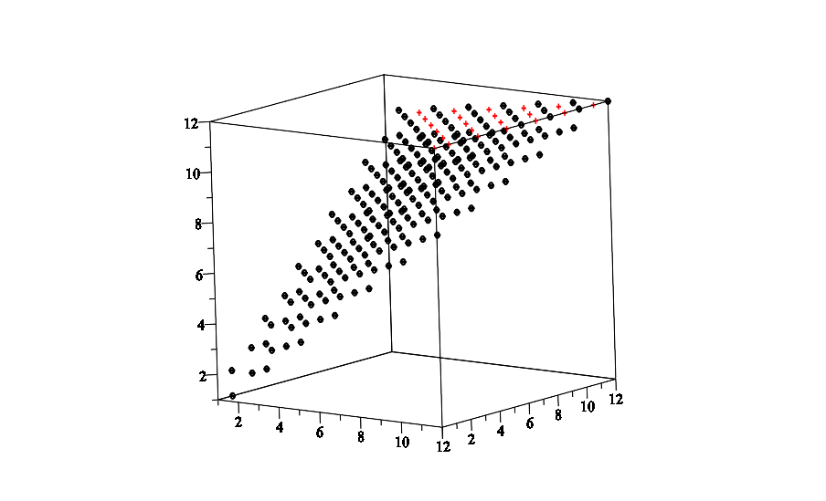
Figure 4: Holes in the Kronecker cone when all three partitions are of length 2. The point at $(i,j,k)$ is black if $g_{(24-i,i)(24-j,j)(24-k,k)}$ is nonzero (assuming, $j\leq i\leq k\leq 24/2$). The points with red crosses, or no dots are 0. Note that the top face has both zero and nonzero values. These are the holes in the polytope.

The sequence $g_{(k,k),(k,k),(k,k)}$, for $k\geq 0$ illustrates that the Kronecker coefficients cannot possibly count points in the dilations of a polytope because such sequences are necessarily weakly increasing. That is, the Kronecker function does not count integer points in polytopes. See [Kin09, BOR09b] for related results and conjectures.

Remark 14 (The holes of the Kronecker cone).

Example 13 illustrates the origin of the holes in the Kronecker cone in Figure 4. Note that the holes are all in the face of the Kronecker cone defined by equations $\mu_{1}=\mu_{2}$, $\nu_{1}=\nu_{2}$, $\lambda_{1}=\lambda_{2}$, $\lambda_{3}=\lambda_{4}=0$. It is always the case that the zeros of the Kronecker cone are on its walls (facets) [Man15].

This can also be seen for the example in Figure 4 where the holes are all inside the face defined by $\lambda_{1}=\lambda_{2}$.

Example 15.

Consider an example of Baldoni and Vergne [BVW16, Section 5.1.1], whose methods are quite different from ours. Let $\lambda=(132,38,19,11),$ $\mu=(110,90),$ and $\nu=(120,80).$ We will compute an expression for the dilated Kronecker coefficient $g_{k\mu,k\nu,k\lambda}.$

We have $k(\mu_{2}+\nu_{2})=170k,$ $k(\lambda_{3}+\lambda_{4})=30k,$ $k(\lambda_{2}+\lambda_{4})=49k,$ $k\min(\lambda_{2}+\lambda_{3},\lambda_{1}+\lambda_{4})=k\min(57,143)=57k.$ Eqn. (13) of Theorem 7 says that $g_{k\mu,\,k\nu,\,k\lambda}$ is equal to

$$p_{S}(50k,91k)-p_{S}(50k,83k-1)-p_{S}(31k-1,91k-2)+p_{S}(31k-1,64k-2).$$

From Section 2, the last two terms cancel each other because both correspond to Region II in Figure 3, and hence depend only on the first argument $n$ of $p_{S}(n,m).$ The two remaining terms correspond to Region III. The reader can check that using the formula for Region III gives

$$g_{k\mu,k\nu,k\lambda}=52k^{2}+\frac{25}{2}k+\frac{3}{4}+\frac{(-1)^{k}}{4},$$

in agreement with the result in [BVW16, Section 5.1.1].

3.5 Inequalities implying that a Kronecker coefficient is atomic

Analysing the order relations in the exponents appearing in Eqn. (12) yields the following result.

Corollary 16.

Assume $\mu_{2}\geq\nu_{2}.$ The atomic coefficient equals the Kronecker coefficient if

1. $\nu_{2}<\lambda_{3}+\lambda_{4};$ OR

2. 1. $\lambda_{3}+\lambda_{4}\leq\nu_{2}\leq\lambda_{2}+\lambda_{4}$ and

   2. $(\lambda_{3}+\lambda_{4})+(\lambda_{2}+\lambda_{4})\leq\mu_{2}+\nu_{2}\leq(\lambda_{3}+\lambda_{4})+\min(\lambda_{2}+\lambda_{3},\lambda_{1}+\lambda_{4}),$

   OR

3. $\lambda_{2}+\lambda_{3}+2\lambda_{4}=\mu_{2}+\nu_{2}.$

Proof.

We examine the exponents in  (12). Recall that a monomial $y^{b}x^{a}$ will make a nonzero contribution to $g_{\mu,\nu,\lambda}$ if and only if $b\leq\nu_{2}\text{ and }b+a\leq\mu_{2}+\nu_{2}.$

In the first case both the atomic and Kronecker coefficient vanish.

We consider the second case. The two exponents of $y$ in  (12) are ordered as follows:

$$\lambda_{3}+\lambda_{4}<\lambda_{2}+\lambda_{4}+1.$$ (17)

The five distinct exponents of $x$ occurring in (12) satisfy

$$\lambda_{3}+\lambda_{4}-1<\lambda_{2}+\lambda_{4}<\min(\lambda_{2}+\lambda_{3}+1,\lambda_{1}+\lambda_{4}+1)\\ \leq\max(\lambda_{2}+\lambda_{3}+1,\lambda_{1}+\lambda_{4}+1)<\lambda_{1}+\lambda_{3}+2.$$ (18)

Compare with [Ros01]. By considering the sequences of total degree of the 7 monomials in each of the two lines of (12), we have the following two chains of inequalities:

$$\lambda_{2}+\lambda_{3}+2\lambda_{4}<(\lambda_{3}+\lambda_{4})+\min(\lambda_{2}+\lambda_{3}+1,\lambda_{1}+\lambda_{4}+1)\\ \leq(\lambda_{3}+\lambda_{4})+\max(\lambda_{2}+\lambda_{3}+1,\lambda_{1}+\lambda_{4}+1)<(\lambda_{3}+\lambda_{4})+(\lambda_{1}+\lambda_{3}+2);$$ (19)

$$\lambda_{2}+\lambda_{3}+2\lambda_{4}<(\lambda_{2}+\lambda_{4}+1)+\min(\lambda_{2}+\lambda_{3}+1,\lambda_{1}+\lambda_{4}+1)\\ \leq(\lambda_{2}+\lambda_{4}+1)+\max(\lambda_{2}+\lambda_{3}+1,\lambda_{1}+\lambda_{4}+1).$$ (20)

A monomial $y^{b}x^{a}$ will make a nonzero contribution to $g_{\mu,\nu,\lambda}$ if and only if $b\leq\nu_{2}\text{ and }b+a\leq\mu_{2}+\nu_{2}.$ In view of Eqn. (17), the condition on $\nu_{2}$ eliminates the possibility of any contribution to the Kronecker coefficient from the monomials in the second line of (12). Hence the subset of the remaining 4 monomials in Eqn. (12) contributing to the Kronecker coefficient $g_{\mu,\nu,\lambda}$ is determined by where the number $\mu_{2}+\nu_{2}$ falls in the consecutive intervals determined by each of the inequalities Eqn. (19). The bounds on $\mu_{2}+\nu_{2}$ clearly eliminate all but the first monomial, the atomic coefficient, in the first line of (12).

Finally consider the third case, $\lambda_{2}+\lambda_{3}+2\lambda_{4}=\mu_{2}+\nu_{2}.$ Note that $\nu_{2}\geq\lambda_{2}+\lambda_{4}+1$ is impossible because it would force

$$\mu_{2}=(\lambda_{2}+\lambda_{4}-\nu_{2})+(\lambda_{3}+\lambda_{4})\leq(\lambda_{3}+\lambda_{4})-1<\lambda_{2}+\lambda_{4}<\nu_{2}.$$

Hence $\nu_{2}\leq\lambda_{2}+\lambda_{4},$ and we are reduced to the first two cases. This finishes the proof. ∎

From this we can easily deduce some conditions on the parts which ensure that the atomic Kronecker coefficients are an upper bound for the Kronecker coefficients. In fact Theorem 17 below states that NO restrictions on the parts of $\lambda$ are needed, as we will show in the next section.

3.6 The atomic Kronecker coefficient is an upper bound for the Kronecker coefficient for the case $2-2-4$

In this section we show that for a triple of partitions $\lambda,\mu,\nu$ of the same integer, such that $\ell(\lambda)\leq 4,\ell(\mu),\ell(\nu)\leq 2,$ and $\mu_{2}\geq\nu_{2},$ the atomic Kronecker coefficient $\tilde{g}_{\mu,\nu,\lambda}$ is always greater than or equal to the actual Kronecker coefficient $g_{\mu,\nu,\lambda}.$

We use our polyhedral geometry approach to prove this result. Theorem 7 and its applications showed how the Kronecker coefficient is completely determined by the functions $p_{S}(n,m).$ Our proof, depending heavily on the fact that the $p_{S}(n,m)$ are vector partition functions, consists of a careful analysis of the contributions of each term in the polynomial $P_{\lambda}$ in the proof of Theorem 7.

Our arguments will reveal a remarkable relationship between the seven monomials in $P_{\lambda}.$ For brevity we will label the exponents of $y$ and $x$ appearing in Eqn. 12 as follows:

$$b=\lambda_{3}+\lambda_{4},a_{0}=\lambda_{2}+\lambda_{4},a_{1}=\lambda_{2}+\lambda_{3}+1,a_{2}=\lambda_{1}+\lambda_{4}+1,a_{3}=\lambda_{1}+\lambda_{3}+2.$$

Combining Eqns. (17), (18), we have the inequalities

$$b\leq a_{0}<\{a_{1},a_{2}\}<a_{3}.$$ (21)

The polynomial $P_{\lambda}$ is then $P_{\lambda}=y^{b}(x^{a_{0}}-x^{a_{1}}-x^{a_{2}}+x^{a_{3}})+y^{a_{0}+1}(-x^{b-1}+x^{a_{1}}+x^{a_{2}}).$

Recall that the first monomial, $y^{b}x^{a_{0}},$ is the one that determines the atomic Kronecker coefficient. We will call this the atomic monomial. The dependency digraph of Figure 5 for the signed monomials in $P_{\lambda}$ is a consequence of Theorem 7 and the inequalities (21), (19), (20). If $M_{1},$ $M_{2}$ are signed monomials, a directed edge from node $M_{1}$ to node $M_{2}$ in the digraph signifies that if $M_{1}$ makes a nonzero contribution to the Kronecker coefficient (as described by Theorem 7), then so must the monomial $M_{2}$.

Figure 5: Dependency digraph for the monomials in $P_{\lambda}$ (the atomic monomial is in bold). The blue and red arrows correspond to the two scenarios described in the proof of Theorem 17.

We will examine the contribution to $g_{\mu,\nu,\lambda}$ of each of the three non-atomic monomials in $P_{\lambda}$ with positive coefficient. By Eqn. (13) from Theorem 7, this in turn will necessarily entail a detailed analysis of the vector partition function $p_{S}(n,m)$ of Section 2. The final result exhibits the following surprising phenomenon in the monomials of $P_{\lambda}.$ We will show that in fact, every non-atomic monomial with positive coefficient can be matched with a monomial with negative coefficient to yield a net nonpositive value (see the coloured arrows in Figure 5). For clarity of exposition, the technical lemmas have been relegated to the Appendix at the end of the paper.

Theorem 17.

The atomic coefficient is an upper bound for the Kronecker coefficient in the case $2-2-4.$

Proof.

The atomic Kronecker coefficient is determined by only the first monomial $y^{b}x^{a_{0}}.$ In order to prove that the result of the corresponding coefficient extraction from $F_{2,2}$ is never less than the actual Kronecker coefficient, it suffices to show that the contribution of the three remaining (non-atomic) positively signed monomials, viz. $+y^{a_{0}+1}x^{a_{1}},+y^{a_{0}+1}x^{a_{2}},+y^{b}x^{a_{3}}$ is offset by that of the three negative ones, $-y^{b}x^{a_{1}},-y^{b}x^{a_{2}},-y^{a_{0}+1}x^{b-1}.$

More precisely, we say that a positive monomial $+M_{1}$ is offset by a negative monomial $-M_{2}$ if the contribution of $M_{1}-M_{2}$ to the Kronecker coefficient is nonpositive.

Lemmas 30 to 36 in the Appendix will establish that one of the following two scenarios, corresponding respectively to the blue arrows and the red arrows in Figure 5, must occur.

The contribution of

1. $+y^{a_{0}+1}x^{a_{1}}$ is offset by $-y^{b}x^{a_{1}}$ AND

2. $+y^{a_{0}+1}x^{a_{2}}$ is offset by $-y^{a_{0}+1}x^{b-1}$ AND

3. $+y^{b}x^{a_{3}}$ is offset by $-y^{b}x^{a_{2}};$

OR the contribution of

1. $+y^{a_{0}+1}x^{a_{1}}$ is offset by $-y^{a_{0}+1}x^{b-1}$ AND

2. $+y^{a_{0}+1}x^{a_{2}}$ is offset by$-y^{b}x^{a_{2}}$ AND

3. $+y^{b}x^{a_{3}}$ is offset by $-y^{b}x^{a_{1}}.$

The above two scenarios show that, apart from the monomial $y^{b}x^{a_{0}},$ whenever there is a contribution from a positively signed monomial in $P_{\lambda}$ to the Kronecker coefficient, there is an offsetting negatively signed monomial which also contributes, resulting in a net nonpositive contribution.

This completes the proof that the monomial $y^{b}x^{a_{0}}$ gives the maximal contribution to the Kronecker coefficient, i.e. that $\tilde{g}_{\mu,\nu,\lambda}$ is an upper bound. ∎

3.7 Bravyi’s vanishing conditions

Given a partition $\lambda$, denote by $\bar{\lambda}$ the partition obtained from $\lambda$ after deleting its first part. Murnaghan discovered a necessary condition for the Kronecker coefficient $g_{\lambda,\mu,\nu}$ to be nonzero. He showed that the following inequality has to hold:

$$|\bar{\lambda}|\leq|\bar{\mu}|+|\bar{\nu}|,$$ (22)

Note that since the Kronecker coefficients are symmetric under permutations of the index, there are really three inequalities.

The following stronger result (due to Bravyi) follows from our methods. The reader may want to compare with Proposition 5.

Proposition 18 (Bravyi [Kir04, Bra04]).

Assume $\ell(\lambda)\leq 4,\ell(\mu),\ell(\nu)\leq 2.$ The Kronecker coefficient is zero if $\nu_{2}<\lambda_{3}+\lambda_{4}$ or $\mu_{2}+\nu_{2}<\lambda_{2}+\lambda_{3}+2\lambda_{4}.$ Equivalently, if the Kronecker coefficient $g_{\mu,\nu,\lambda}$ is nonzero then Bravyi’s inequalities (11) are satisfied.

Proof.

We assume without loss of generality that $\mu_{2}\geq\nu_{2}.$ We will use the polynomial $P_{\lambda}$ of Theorem 7.

First suppose $\nu_{2}<\lambda_{3}+\lambda_{4}$. Then we have $\nu_{2}<\lambda_{3}+\lambda_{4}\leq\lambda_{2}+\lambda_{4}.$ Examining the polynomial $P_{\lambda}$ in (12), we see that none of the monomials $y^{b}x^{a}$ makes a contribution since the condition $b\leq\nu_{2}$ is violated for both exponents $b$ of $y$ in $P_{\lambda}.$

Now suppose $\mu_{2}+\nu_{2}<\lambda_{2}+\lambda_{3}+2\lambda_{4}.$ Observe that $\lambda_{2}+\lambda_{3}+2\lambda_{4}$ is precisely the sum of the exponents for the first monomials $y^{b}x^{a}$ in each of the first two lines of the polynomial in (12). Hence the condition $b+a\leq\mu_{2}+\nu_{2}$ is violated for these two monomials. But the sum of exponents $b+a$ for each of the other monomials in (12) is strictly greater than the sum for the first monomial in each line, so the condition is violated for all the monomials in $P_{\lambda}.$ ∎

3.8 A closed formula for the reduced Kronecker coefficients

Murnaghan also observed that the sequences of Kronecker coefficients $\big{(}g(\lambda+(k),\mu+(k),\nu+(k))\big{)}_{k\geq 0}$ always stabilize. Their stable value is known as the reduced Kronecker coefficient and denoted by $\bar{g}_{\bar{\lambda},\bar{\mu},\bar{\nu}}$, where, given a partition $\lambda$, we denote by $\bar{\lambda}$ the partition obtained from $\lambda$ deleting its first part.

Proposition 19.

Let $\lambda_{2}\geq\mu_{2}\geq\nu_{2}.$ Assume $\lambda$ has at most two parts. Then $g_{\mu,\nu,\lambda}$ is independent of $\lambda_{1}$ as soon as $\lambda_{1}\geq\mu_{2}+\nu_{2}.$ Moreover, the stable value is $p_{S}(\nu_{2},\nu_{2}+\mu_{2}-\lambda_{2})-p_{S}(\nu_{2},\nu_{2}+\mu_{2}-\lambda_{2}-1).$ Explicitly, let $\ell=\nu_{2}+\mu_{2}-\lambda_{2}.$ Then:

$$\bar{g}_{(\lambda_{2}),(\mu_{2}),(\nu_{2})} =\begin{cases}\frac{\ell}{2}+\frac{3+(-1)^{\ell}}{4}=\left\lfloor\frac{\ell}{2}\right\rfloor+1&\text{ if }\mu_{2}+\nu_{2}\geq\lambda_{2}\\ 0&\text{ if }\mu_{2}+\nu_{2}<\lambda_{2}\end{cases}$$ (23)

Proof.

We have $\lambda_{3}=\lambda_{4}=0.$ For any statement $S$, we write $\delta(S)$ to mean 1 if $S$ is true and 0 otherwise. From Eqn. (13) of Theorem 7, the Kronecker coefficient is

$$p_{S}(\nu_{2},\nu_{2}+\mu_{2}-\lambda_{2})-p_{S}(\nu_{2},\nu_{2}+\mu_{2}-(\lambda_{2}+1))\\ -p_{S}(\nu_{2},\nu_{2}+\mu_{2}-(\lambda_{1}+1))\cdot{\scriptstyle\mathbf{\delta(\mu_{2}+\nu_{2}\geq\lambda_{1}+1)}}+p_{S}(\nu_{2},\nu_{2}+\mu_{2}-(\lambda_{1}+2))\cdot{\scriptstyle\mathbf{\delta(\mu_{2}+\nu_{2}\geq\lambda_{1}+2)}}\\ -p_{S}(\nu_{2}-(\lambda_{2}+1),\nu_{2}-(\lambda_{2}+1)+\mu_{2}+1)+p_{S}(\nu_{2}-(\lambda_{2}+1),\nu_{2}-(\lambda_{2}+1)+\mu_{2}-(\lambda_{2}+1))\\ +0\cdot p_{S}(\nu_{2}-(\lambda_{2}+1),\nu_{2}-(\lambda_{2}+1)+\mu_{2}-(\lambda_{1}+1))$$

The zero coefficient in the last line is explained by the fact that $(\lambda_{1}+\lambda_{2})/2\geq\mu_{2}\geq\nu_{2},$ and thus we always have $\mu_{2}+\nu_{2}\leq\lambda_{1}+\lambda_{2}.$

The hypothesis that $\lambda_{1}\geq\mu_{2}+\nu_{2}$ eliminates the two terms with $\lambda_{1}$ in their arguments, establishing a stable value. The reduced Kronecker coefficient is thus given by

$$\mathbf{p_{S}}(\nu_{2},\nu_{2}+\mu_{2}-\lambda_{2})-\mathbf{p_{S}}(\nu_{2},\nu_{2}+\mu_{2}-(\lambda_{2}+1))\\ -\mathbf{p_{S}}(\nu_{2}-(\lambda_{2}+1),\nu_{2}+\mu_{2}-\lambda_{2})+\mathbf{p_{S}}(\nu_{2}-(\lambda_{2}+1),\nu_{2}+\mu_{2}-2(\lambda_{2}+1))$$ (24)

Of these four terms, since $\lambda_{2}\geq\mu_{2}\geq\nu_{2},$ the third and fourth terms are immediately eliminated because the first argument is negative: $\nu_{2}-\lambda_{2}-1\leq-1.$

If $\mu_{2}+\nu_{2}<\lambda_{2},$ both first and second terms are identically zero.

If $\mu_{2}+\nu_{2}=\lambda_{2},$ only the first term appears, but it must be 1 from the boundary values $p_{S}(n,0)=1=p_{S}(0,m)$ recorded in Section 3.3.

If $\mu_{2}+\nu_{2}>\lambda_{2},$ the first two vector partition functions both appear. Since $\lambda_{2}-\mu_{2}\geq 0$ implies $\nu_{2}\geq\ell=\nu_{2}+\mu_{2}-\lambda_{2},$ both are computed using the quasipolynomial corresponding to Region I in Figure 3, and consequently the reduced Kronecker coefficient is

$$\mathbf{p_{S}}(\nu_{2},\ell)-\mathbf{p_{S}}(\nu_{2},\ell-1)=\frac{\ell}{2}+\frac{3+(-1)^{\ell}}{4}.$$

The proof is now complete. ∎

Using the symmetry of the Kronecker coefficients with respect to the three partitions, we immediately have:

Figure 6: The chamber complex for the reduced Kronecker coefficients indexed by three one–row shapes. The reduced coefficients are zero outside the tetrahedra, one on all the boundaries, and grow linearly as we move towards the center of one of the chambers. The interior of the cone is divided into three chambers.

Corollary 20.

Fix $\lambda_{2},\mu_{2},$ and $\nu_{2}$. Let $a=\max(\lambda_{2},\mu_{2},\nu_{2})\geq b\geq c=\min(\lambda_{2},\mu_{2},\nu_{2})$ be a total ordering of $\lambda_{2},\mu_{2},\nu_{2}.$ Set $\ell=b+c-a.$ Then

$$\bar{g}_{(\lambda_{2}),(\mu_{2}),(\nu_{2})} =\bar{g}_{(a),(b),(c)}=\begin{cases}\frac{\ell}{2}+\frac{3+(-1)^{\ell}}{4}=\left\lfloor\frac{\ell}{2}\right\rfloor+1&\text{ if }\ell\geq 0\\ 0&\text{ if }\ell<0.\end{cases}$$ (25)

The chamber complex for this quasipolynomial is illustrated in Figure 6. The walls are the hyperplanes $I):\mu_{2}+\nu_{2}=\lambda_{2}$, $II):\mu_{2}+\lambda_{2}=\nu_{2}$, $III):\lambda_{2}+\nu_{2}=\mu_{2}.$ The reduced Kronecker coefficient indexed by points on any of these walls always has value equal to one.

We have obtained the counting function for the number of integer points in the one-dimensional polytope of Figure 1, which was studied in Example 1.

3.9 The relative positions of the cones associated to the Kronecker, the reduced Kronecker and the Littlewood–Richardson coefficients

Identify a triple of partitions of lengths $\leq a,b,c$ (respectively) with a point in $\mathbb{Q}^{a+b+c}$. The set of triples of partitions whose corresponding Kronecker coefficient is nonzero is known to have the structure of a finitely generated semigroup ([Chr06, Kly04, Man15]). This semigroup generates a rational polyhedral cone, called the Kronecker cone and denoted by $PKron_{a,b,c}$. Its walls (i.e. facets) are described by a finite set of inequalities. Can we find these inequalities? Is this cone saturated, or do there exist holes, that is, points where the Kronecker coefficient is zero, inside it? If so, where are the holes located? What is the relation between the Kronecker coefficients and other important families of coefficients such as the Littlewood–Richardson coefficients or the reduced Kronecker coefficients.

We will use an unexpected discovery of Murnaghan to explore these issues: In the particular case where $\bar{\lambda}=\bar{\mu}+\bar{\nu}$ (that is, when Eq (22) is an equality), and when the first parts of the partitions are “big enough”, the Kronecker coefficient $g_{\lambda,\mu,\nu}$ coincides with the Littlewood-Richardson coefficient $c^{\bar{\lambda}}_{\bar{\mu},\bar{\nu}}$. Equivalently, Murnaghan’s result can be expressed in terms of the reduced Kronecker coefficients, $\bar{g}_{\bar{\lambda},\bar{\mu},\bar{\nu}}=c_{\bar{\lambda},\bar{\mu},\bar{\nu}}$.

Given a family of coefficients indexed by triples of partitions, we define a cone (with the same name) as the polyhedral cone generated by its nonzero values. We ask for the relation between the positions of these different cones (the Kronecker, the reduced Kronecker, and the Littlewood–Richardson coefficients) inside of the atomic cone.

The atomic Kronecker coefficients attain their minimum nonzero value (one) at its boundary: $\mu_{2}+\nu_{2}-\lambda_{2}-\lambda_{3}-2\lambda_{4}=0$ or $\nu_{2}-\lambda_{3}-\lambda_{4}=0$ (compare with inequality (11)). Being the solution of a vector partition function problem, it follows that when we dilate the three indexing partitions, the values of the atomic Kronecker coefficients inside the cone are always increasing.

Remark 21.

On the face defined by $\mu_{2}+\nu_{2}-\lambda_{2}-\lambda_{3}-2\lambda_{4}=0$, the atomic Kronecker coefficient coincides with the Kronecker coefficient; see Corollary 16. Furthermore, they are always equal to one. A triple of partitions $(\lambda,\mu,\nu)$ of the same weight is stable if $g_{(k\lambda,k\mu,k\nu)}$ equals 1 for all $k.$ We have shown that all Kronecker coefficients corresponding to triples in this face are stable triples. Stable triples are relevant because the sequences $g_{\alpha+n\lambda,\beta+n\mu,\gamma+\nu}$ stabilize for $n$ sufficiently large, see [Ste14].

Theorem 22.

The Littlewood–Richardson cone coincides with the intersection of the hyperplane $\lambda_{4}=0$ and the face of the Kronecker cone defined by the first Bravyi inequality, $\lambda_{2}+\lambda_{3}+2\lambda_{4}=\mu_{2}+\nu_{2}$.

Proof.

Let $c_{\alpha,\beta}^{\gamma}=\bar{g}_{\alpha,\beta}^{\gamma}=g_{\lambda,\mu,\nu}$ with $\alpha=\bar{\mu}$, $\beta=\bar{\nu}$ and $\gamma=\bar{\lambda}$. We want to see where $(\lambda,\mu,\nu)$ sits in relation with the Kronecker cone.

Suppose that $c_{\alpha,\beta}^{\gamma}>0$. Since $\alpha$ and $\beta$ have just one part, Pieri’s rule tells us that the length of $\gamma$ can be at most two, and hence $\lambda_{4}=0$, and $\lambda_{2}+\lambda_{3}=\mu_{2}+\nu_{2}$. On the other hand, using the inequalities described in Corollary 16 we easily see that all atomic Kronecker coefficients in this wall are indeed Kronecker coefficients.

Let $N$ be any number such that the triple of sequences $(N-\lambda_{2},\lambda_{2},\lambda_{3}),(N-\mu_{2},\mu_{2}),(N-\nu_{2},\nu_{2})$ are partitions. It remains to see whether $g_{(N-\lambda_{2},\lambda_{2},\lambda_{3}),(N-\mu_{2},\mu_{2}),(N-\nu_{2},\nu_{2})}$ is reduced. For this, we will use the bound described in Theorem 1.5 of [BOR11]. It says that such a Kronecker coefficient is stable as soon as $N\geq\lambda_{2}+\mu_{2}+\nu_{2}+\left\lfloor\frac{\lambda_{3}}{2}\right\rfloor=2\lambda_{2}+\left\lfloor\frac{\lambda_{3}}{2}\right\rfloor$. But since $(N-\lambda_{2},\lambda_{2},\lambda_{3})$ has to be a partition, the smallest possible value for $N$ will be that one that corresponds to partition $(\lambda_{2},\lambda_{2},\lambda_{3})$. That is, $2\lambda_{2}+\lambda_{3}\geq 2\lambda_{2}+\left\lfloor\frac{\lambda_{3}}{2}\right\rfloor.$ ∎

We ask for the position of those nonzero Littlewood–Richardson coefficients (inside the Kronecker cone) coming from the identities: $g_{\mu,\nu,\lambda}=\bar{g}_{\bar{\mu},\bar{\nu},\bar{\lambda}}=c_{\bar{\mu},\bar{\nu}}^{\bar{\lambda}}.$ Now the Littlewood-Richardson coefficient $c^{(\lambda_{2},\lambda_{3})}_{(\mu_{2}),(\nu_{2})}$ is nonzero iff the skew-shapes $(\lambda_{2},\lambda_{3})/(\mu_{2})$ and $(\lambda_{2},\lambda_{3})/(\nu_{2})$ are horizontal strips, or equivalently iff $\lambda_{2}\geq\mu_{2}\geq\lambda_{3}\text{ and }\lambda_{2}\geq\nu_{2}\geq\lambda_{3},$ which in turn is equivalent to saying $\mu_{2}$ and $\nu_{2}$ lie in the interval $[\lambda_{3},\lambda_{2}].$ Hence, when the LR coefficient is nonzero, we must have (since $\lambda_{1}\geq\lambda_{2}\geq\lambda_{3}\geq\lambda_{4}$),

$$|\mu_{2}-\nu_{2}|\leq\lambda_{2}-\lambda_{3}\leq\min(\lambda_{1}-\lambda_{3},\lambda_{2}-\lambda_{4}).$$

We have recovered another result of Bravyi, his third, and last, inequality.

Remark 23.

We have the following implications. If a Kronecker coefficient is atomic then it is reduced, the reason being that the value of $\tilde{g}$ does not depend on the first part of $\lambda$. On the other hand, if a Kronecker coefficient satisfies the equality of Murnaghan’s condition, then it is reduced. This is Theorem 22.

4 The vector partition function $F_{n,m}$

Having completed our analysis of the $n=m=2$ case, we examine the extent to which these results generalize. First we show that we can make a variable substitution to convert $\frac{{a_{\delta_{n}}[X]}{a_{\delta_{m}}[Y]}}{a_{\delta_{nm}}[XY]}$ into a vector partition function. This is the result of Theorem 26.

Let $S(p)$ denote the smallest monomial in $p$ with respect to the lexicographic order. Repeating the reasoning given for the case $n=m=2$ in Section 3, we obtain for the general situation the following identity:

$$\frac{{a_{\delta_{n}}[X]}{a_{\delta_{m}}[Y]}}{a_{\delta_{nm}}[XY]}S(a_{\lambda+\delta_{nm}}[XY]) =\sum_{\mu,\nu}\tilde{g}_{\mu,\nu,\lambda}\,S(a_{\mu+\delta_{n}}[X])S(a_{\nu+\delta_{m}}[Y])+\text{lex. gr.}$$ (26)

We proceed by first expanding all the Vandermonde determinants involved as a product of linear binomial factors. We want to factor the binomial terms so that we obtain a product of terms of the form $(1-M)$ where $M$ is a Laurent monomial. We can do this in such a way that the resulting Laurent series converges in a nonzero domain if we follow the lexicographic ordering, and always factor the smallest monomial in each binomial. The argument is similar to the one for $F_{2,2},$ see the discussion following  (8).

We consider the special alphabets $X=\{1,x_{1},x_{2},\ldots,x_{n-1}\},\quad$ $Y=\{1,y_{1},y_{2},\ldots,y_{m-1}\},n,m\geq 2.$ Then $XY=\{1,x_{i},y_{j},x_{i}y_{j}:1\leq i\leq n-1,1\leq j\leq m-1\}.$ The set $XY$ is ordered as follows:

$$1>x_{i}>x_{i+1},y_{j}>y_{j+1},x_{i}>y_{j},x_{i}y_{j}>x_{k}y_{\ell}\text{ if }i<k,\text{ or }i=k\text{ and }j<l.$$ (27)

The following claim is clear.

Lemma 24.

The smallest term in $S(a_{\lambda+\delta_{nm}}[XY])$, with respect to the lexicographic ordering, is the product of the monomials in the main diagonal of the matrix of the alternant $a_{\lambda+\delta_{nm}}[XY].$

Similarly, to compute the smallest term, with respect to the lex ordering, in each of the two remaining alternants $S(a_{\mu+\delta_{n}}[X])$ and $S(a_{\nu+\delta_{m}}[Y])$, we take the product of the monomials in the main diagonal of the corresponding matrices. We obtain a Laurent series

$$\sum_{\mu,\nu}g_{\mu,\nu,\lambda}\,{\bf x}^{\,\,\,l_{1}(\mu,\nu,\lambda)}{\bf y}^{\,\,\,l_{2}(\mu,\nu,\lambda)}$$

where $l_{1}(\mu,\nu,\lambda)$ and $l_{2}(\mu,\nu,\lambda)$ are linear combinations of the parts of $\mu,\nu$ and $\lambda$. It is a product of binomial terms of the form 1 minus a Laurent monomial. Finally, we perform a change of basis which we describe in detail below, to ensure that we get a convergent Taylor series expansion.

For example, for $n=m=3$, the substitution is $x_{1}=s_{1}t_{1},$ $x_{2}=s_{1}s_{2}t_{1}^{2},$ $y_{1}=s_{0}s_{1}s_{2}t_{1}^{2},$ and $y_{2}=s_{0}s_{1}s_{2}t_{1}^{3}$ More precisely, in order to guarantee convergence of our series, we assume in Eqn. (27) that $1>|x_{1}|>|x_{2}|>..>|x_{n-1}|>|y_{1}|>|y_{2}|>...>|y_{m-1}|>|x_{1}y_{1}|>|x_{1}y_{2}|>...>|x_{1}y_{m-1}|\\ \ldots>|x_{n-1}y_{1}|>|x_{n-1}y_{2}|>...>|x_{n-1}y_{m-1}|$.

We define the rational function $G_{n,m}$ by $G_{n,m}=\frac{{a_{\delta_{n}}[X]}{a_{\delta_{m}}[Y]}}{a_{\delta_{nm}}[XY]}.$ Observe that we have the Vandermonde expansion

$$a_{\delta_{n}}[X]=\prod_{i=1}^{n-1}(1-x_{i})\prod_{1\leq i<j\leq n-1}(x_{i}-x_{j}),$$

and similarly for the second alternant $a_{\delta_{m}}[Y].$ For the alternant in the denominator we have $a_{\delta_{nm}}[XY]=a_{\delta_{n}}[X]\cdot a_{\delta_{m}}[Y]\cdot A\cdot B\cdot C\cdot D\cdot E\cdot F,$ where

$$A=\prod_{j=1}^{m-1}\prod_{i=1}^{n-1}(x_{i}-y_{j}),\,\,B=\prod_{i=1}^{n-1}\prod_{j=1}^{m-1}(1-x_{i}y_{j})$$

and $C=\prod_{i=1}^{n-1}\prod_{j=1}^{m-1}(x_{i}-x_{i}y_{j})\cdot\prod_{j=1}^{m-1}\prod_{i=1}^{n-1}(y_{j}-x_{i}y_{j})$

$$=\left(\prod_{j=1}^{m-1}(1-y_{j})\right)^{n-1}(\prod_{i=1}^{n-1}x_{i}^{m-1})\cdot\left(\prod_{i=1}^{n-1}(1-x_{i})\right)^{m-1}(\prod_{j=1}^{m-1}y_{j}^{n-1}),$$

$$D=\prod_{\stackrel{{\scriptstyle k=1}}{{k\neq i}}}^{n-1}\prod_{i=1}^{n-1}\prod_{j=1}^{m-1}(x_{k}-x_{i}y_{j})\cdot\prod_{\stackrel{{\scriptstyle k=1}}{{k\neq j}}}^{m-1}\prod_{j=1}^{m-1}\prod_{i=1}^{n-1}(y_{k}-x_{i}y_{j}),\qquad E=\prod_{j\neq\ell=1}^{m-1}\prod_{1\leq i<k\leq n-1}(x_{i}y_{j}-x_{k}y_{\ell}),$$

$$F=\prod_{j=1}^{m-1}\prod_{1\leq i<k\leq n-1}(x_{i}y_{j}-x_{k}y_{j})\cdot\prod_{i=1}^{n-1}\prod_{1\leq j<\ell\leq m-1}(x_{i}y_{j}-x_{i}y_{\ell})\\ =\prod_{j=1}^{m-1}y_{j}^{n-1\choose 2}\prod_{1\leq i<k\leq n-1}(x_{i}-x_{k})^{m-1}\cdot\prod_{i=1}^{n-1}x_{i}^{m-1\choose 2}\prod_{1\leq j<\ell\leq m-1}(y_{j}-y_{\ell})^{n-1}.$$

It follows that the quotient of alternants $G_{n,m}$ simplifies to $\dfrac{1}{ABCDEF}.$

Note that each factor in $A,C,D,E,F$ can be rewritten in the form $(1-M)$ where $M$ is a Laurent monomial in the $x_{i}$ and the $y_{j}.$ The factors of $B$ are already in this form. For instance, in $E$ we can rewrite each factor as $x_{i}y_{j}-x_{k}y_{\ell}=x_{i}y_{j}(1-x_{k}y_{\ell}x_{i}^{-1}y_{j}^{-1}).$

Thus, the following definition for $\bar{F}_{n,m}(X,Y)$ makes sense.

Definition 25 ($\bar{F}_{n,m}(X,Y)$ ).

There are positive integers $a_{i},b_{j}$ such that in the product

$$G_{n,m}\prod_{i=1}^{n-1}x_{i}^{a_{i}}\prod_{i=j}^{m-1}y_{j}^{b_{j}},$$

all factors are of the form $(1-M)^{-1}$ where $M$ is a Laurent monomial in the $x_{i}$ and the $y_{j}.$ We define $\bar{F}_{n,m}(X,Y)$ to be this product, i.e. we have

$$G_{n,m}\prod_{i=1}^{n-1}x_{i}^{a_{i}}\prod_{i=j}^{m-1}y_{j}^{b_{j}}=\bar{F}_{n,m}.$$ (28)

We now show that there is a different set of $(n+m-2)$ variables $s_{i},i=0,\ldots n-1,t_{j},j=1,\ldots,m-2,$ such that by effecting a judicious (and non-obvious) change of variables, $\bar{F}_{n,m}(X,Y)$ becomes a product of factors of the form $(1-M)^{-1}$ where each Laurent monomial $M$ in $X,Y$ is a monomial with nonnegative exponents in the new variables $S,T.$ In other words, $F_{n,m}(S,T)$ is a vector partition function in the new variables.

We claim that the quotients of consecutive terms in the sequence (27) become monomials (and not Laurent monomials), after setting, for each $1\leq i\leq n-1$ and $1\leq j\leq m-1$,

$$\begin{cases}&x_{i}=s_{1}s_{2}..s_{i}(t_{1}t_{2}...t_{m-2})^{i}\\ &y_{j}=(s_{0}s_{1}...s_{n-1})(t_{1}t_{2}...t_{m-2})^{n-1}t_{1}t_{2}...t_{j-1}\\ \end{cases}.$$ (29)

Note when $n=m=2$, there are no $t_{i}$ variables, and we recover the substitution for $F_{2,2}$ in Section 2. We have

$$\frac{x_{i+1}}{x_{i}}=s_{i+1}t_{1}t_{2}...t_{m-2},\quad\frac{y_{j+1}}{y_{j}}=t_{j},\ 1\leq j\leq m-2,\\ \frac{y_{1}}{x_{n-1}}=s_{0},\quad\frac{x_{1}y_{1}}{y_{m-1}}=s_{1},\ \frac{x_{i}y_{1}}{x_{i-1}y_{m-1}}=s_{i},\ 2\leq i\leq n-1.$$ (30)

This establishes our claim. Hence we have proved:

Theorem 26.

Let $F_{n,m}(S,T)$ be the series obtained after performing the previous substitutions in the series (28); its domain of convergence is $\{|s_{i}|<1,|t_{j}|<1:0\leq i\leq n-1,1\leq j\leq m-2\}.$ Then $F_{n,m}$ is a vector partition function.

From the preceding discussion we can also conclude:

Corollary 27.

Let $A_{n,m}$ be the matrix associated to the vector partition function $F_{n,m}$, as in Section 2. Then

1. the largest entry is $2n-1;$

2. the number of columns is $\binom{nm}{2}-\binom{n}{2}-\binom{m}{2}$;

3. the number of rows is $m+n-2;$

4. all the basis vectors appear in the columns of $A_{n,m};$

5. the rank of the matrix is $m+n-2.$

Proof.

The largest entry is obtained by examining the largest possible exponent of the variables $s_{i}$ or $t_{j}$ in the monomials $M$ occurring in the factors $(1-M)$ of $F_{n,m}.$ We have, from the product $B$ of the preceding proof, for $i\leq n-2,j\leq m-1,$ the monomial

$$x_{i}y_{j}=(s_{1}\ldots s_{i})(t_{1}t_{2}\ldots t_{m-2})^{i}\cdot(s_{0}s_{1}\ldots s_{n-1})(t_{1}t_{2}\ldots t_{m-2})^{n-1}(t_{1}t_{2}\ldots t_{j-1})$$

and clearly the largest exponent here occurs for each of $t_{1},\ldots,t_{j-1},$ and it equals $i+(n-1)+1=n+i\leq 2n-1.$ The maximum exponent $2n-1$ occurs in the monomial $x_{n-1}y_{j}.$ Examining the products other than $B,$ we see that all other monomials involve dividing by $x_{i}$ or $y_{j}$ or both, so it is clear that they cannot yield a larger exponent.

The number of columns in the matrix $A_{n,m}$ equals the number of linear factors in $a_{\delta_{nm}}[XY]$ minus the number of linear factors in $a_{\delta_{n}}[X]$ minus the number of linear factors in $a_{\delta_{m}}[Y];$ since these are all Vandermonde determinants, the second result follows. For the third result, observe that the number of rows is simply the number of variables in the set $\{s_{i},0\leq i\leq n-1,t_{j},1\leq j\leq m-2\}.$

For the last two statements, observe that Eqn.(30) in the preceding proof establishes that all the basis vectors appear as columns of the matrix $A_{n,m}$, since all the variables $s_{i}$ and $t_{j}$ occur as quotients when converting the factors of the Vandermonde in the products $A$-$F$ into the form $(1-M)$ in Eq. (30). Hence the rank is the number of rows of the matrix. ∎

4.1 The degree of the Kronecker quasipolynomial

We have shown that the Kronecker function $\kappa_{n,m,nm}$ is a quasipolynomial on affine domains. However, a deep theorem of Meinrenken and Sjamaar [MS99] says that $\kappa_{n,m,nm}$ is in fact a piecewise quasipolynomial. This result seems to be unattainable by our methods. However, we immediately obtain information about the degree of the Kronecker quasipolynomial $\kappa_{n,m,nm}$. Let $X$ be an alphabet of size $n$, and $Y$ an alphabet of size $m$, and let

$$d =\frac{n^{2}m^{2}}{2}-\frac{n^{2}}{2}-\frac{m^{2}}{2}-\frac{nm}{2}-\frac{n}{2}-\frac{m}{2}+2$$

Theorem 28.

The degree of the piecewise quasipolynomial Kronecker function $\kappa_{n,m,nm}$ is always $\leq d$.

Proof.

The degree of $\kappa_{n,m,nm}$ is bounded by the dimension of the null space of $A_{n,m}.$ It is thus equal to the number of columns minus the rank. By Corollary 27, this is just $d.$

Since Kronecker coefficients are linear combinations of different shifts of this vector partition function, these bounds apply in general. ∎

The degree of $\kappa_{n,m,nm}$ has been obtained by Baldoni, Vergne, and Walter [BVW16, VW17] using the language of moment maps.

In addition to being completely elementary, another advantage of our approach is that the dimension of the polyhedral cones and their ambient spaces involved in the calculation are the minimal possible ones, as they coincide with the degree of the quasipolynomial.

Example 29.

The domain of convergence of the vector partition function $F_{2,3}$ is $|x_{1}y_{2}|<|x_{1}y_{1}|<|y_{2}|<|y_{1}|<|x_{1}|<1.$ $F_{2,3}$ counts nonnegative integer solutions to $A_{2,3}{\bf x}={\bf n}$, with $A_{2,3}$ equal to

$$\left(\begin{array}[]{rrrrrrrrrrrr}1&0&0&1&0&0&1&0&1&1&1\\ 0&1&0&0&1&1&1&1&1&2&2\\ 0&0&1&1&1&1&1&2&2&2&3\end{array}\right)$$

The dimension of the solution space is rather large. The polytopes involved have dimension $8,$ making them very hard to visualize. However, some interesting phenomena can be observed by looking at the restriction of this system of equations to the positive orthant. Recall that we are looking for nonnegative solutions to $A_{2,3}{\bf x}={\bf n}$. Let ${\bf n}=(n_{1},n_{2},n_{3})$.

If $n_{3}=0$ , since we are only considering nonnegative linear combinations of the columns of the matrix, none of the columns other than the first two can appear. We obtain the restricted matrix $A_{3}=\left(\begin{array}[]{rr}1&0\\ 0&1\end{array}\right)$, and $p_{A_{3}}(n_{1},n_{2})=1$ is a constant polynomial. Here we use the notation of Section 2 for the quasipolynomial $p_{A}({\mathbf{b}})$ associated to the polytope defined by the solution space of the matrix equation $A{\bf x}={{\mathbf{b}}}.$

On the other hand, if $n_{2}=0$, we can discard any column where the second entry is not zero. In this case the restricted matrix is $A_{2}=\left(\begin{array}[]{rrr}1&0&1\\ 0&1&1\end{array}\right)$, and $p_{A_{2}}(n_{1},n_{3})$ is a linear polynomial: We need to solve the system of inequalities $x_{3}\leq n_{1},x_{3}\leq n_{3}$. Hence $p_{A_{2}}(n_{1},n_{3})=1+\min(n_{1},n_{3}).$

Finally, if $n_{1}=0$, the restricted matrix is $A_{1}=\left(\begin{array}[]{rrrrr}1&0&1&1&1\\ 0&1&1&1&2\end{array}\right)$, and $p_{A_{1}}(n_{2},n_{3})$ is a cubic quasipolynomial.

Note that the atomic Kronecker coefficients are identically one only on the facet defined by $n_{3}=0$. Contrast this with the situation for $F_{2,2}$, where the coefficients are identically one on both facets: from Figure 3, we see that $p_{A_{2,2}}(n,m)=1$ if $n=0$ or $m=0.$

5 Appendix: Lemmas for the proof of Theorem 17

We now establish the technical lemmas needed on the monotonic behaviour of the function $p_{S}(n,m)$, in order to prove Theorem 17. For brevity, throughout these arguments, we will write $c(m)$ for the expression $\frac{7}{8}+\frac{(-1)^{m}}{8}.$ Note that $c(m)\leq 1$ for all $m.$

Lemma 30.

The partition function $p_{S}(n,m)$ satisfies

$$p_{S}(n,m)\leq p_{S}(n,m^{\prime})=\binom{n+2}{2}\text{ whenever }m^{\prime}\geq 2n.$$

Proof.

We have three cases.

Case 1: Suppose $n\in[0,\frac{m}{2}].$ Then we claim that $p_{S}(n,m)=\binom{n+2}{2}=p_{S}(n,m^{\prime})$ for all $m^{\prime}\geq 2n.$ This is just a consequence of the definition.

Case 2: Suppose $n\in(\frac{m}{2},m).$ We must show that $p_{S}(n,m)\leq p_{S}(n,m^{\prime})$ for all $m^{\prime}\geq 2n.$

From Figure 3, when $\frac{m}{2}\leq n<m,$ $p_{S}(n,m)$ is given by the formula for Region III, while $p_{S}(n,m^{\prime})$ is given by the binomial coefficient $\binom{n+2}{2}.$ Inspecting the third figure in Figure 2, and using the fact that the $p_{S}(n,m)$ count lattice points in the appropriate regions, it is immediate that the difference $p_{S}(n,m^{\prime})-p_{S}(n,m)$ is nonnegative for $n$ in this interval and $m^{\prime}\geq 2n.$

Case 3: Suppose $n\geq m\geq 0.$ We must show that $p_{S}(n,m)\leq\binom{n+2}{2}=p_{S}(n,m^{\prime})$ for all $m^{\prime}\geq 2n.$ Again this is immediate by the same geometric argument, inspecting the first and third figures in Figure 2.

∎

Lemma 31.

Suppose $\frac{m}{2}<\frac{M}{2}<n<m<M.$ Then $p_{S}(n,M)-p_{S}(n,m)\geq 0.$

Proof.

Both partition functions are computed according to the formula for Region III in Figure 3, and hence count lattice points in a convex polytope (see Figure 2). They are therefore increasing functions in each argument. ∎

Lemma 32.

Fix $k\geq 0.$ Then $p_{S}(n,n+k),$ for $0\leq k\leq n,$ is an increasing function of $n.$

Proof.

From Section 2, we see that the conditions on $k,n,$ imply that $p_{S}(n,n+k)$ corresponds to Region III in Figure 3. As before, since the function $p_{S}(n,n+k)$ counts lattice points in a convex polytope (see the third figure in Figure 2), it is an increasing function of $n.$ ∎

Consider first the monomial $+y^{a_{0}+1}x^{a_{i}},i=1,2.$ Note the crucial fact that from the dependency relations, if either of these monomials contributes a nonzero coefficient, so does the preceding negative monomial $-y^{a_{0}+1}x^{b-1}.$

Lemma 33.

Let $i=1,2.$ Then the net contribution of the monomials $y^{a_{0}+1}(-x^{b-1}+x^{a_{i}})$ to $g_{\mu,\nu,\lambda}$ is negative or zero.

Proof.

The value contributed to $g_{\mu,\nu,\lambda}$ by the monomial $+y^{a_{0}+1}x^{a_{i}},i=1,2,$ is the coefficient $[x^{\mu_{2}}y^{\nu_{2}}]$ in the product $+y^{a_{0}+1}x^{a_{i}}\bar{F}_{2,2},$ which in turn is given by the vector partition function

$$p_{S}(\nu_{2}-(a_{0}+1),\nu_{2}-(a_{0}+1)+(\mu_{2}-a_{i})).$$ (31)

On the other hand, the contribution from the negative monomial $-y^{a_{0}+1}x^{b-1}$ was shown in the proof of Theorem 7 to be coming from Region II in Figure 3. It therefore contributes the value

$$-p_{S}(\nu_{2}-(a_{0}+1),\nu_{2}-(a_{0}+1)+(\mu_{2}-b+1))=-{\nu_{2}-(a_{0}+1)\choose 2}.$$ (32)

But now Lemma 30 says the net contribution of these two monomials is negative or zero, as claimed. ∎

However, this is of course not sufficient to establish our theorem, because both positive monomials $+y^{a_{0}+1}x^{a_{i}},i=1,2$ can make a nonzero contribution. Appealing to the dependency relations, we see that a positive contribution from $+y^{a_{0}+1}x^{a_{i}}$ forces a negative contribution from the monomial $-y^{b}x^{a_{i}},$ for each $i=1,2.$

Lemma 34.

If $\mu_{2}-a_{i}\leq 0,$ then the net contribution of $+y^{a_{0}+1}x^{a_{i}}$ and $-y^{b}x^{a_{i}}$ is negative or zero.

Proof.

The contribution of $+y^{a_{0}+1}x^{a_{i}}$ is given by the vector partition function Eqn. (31), while that of $-y^{b}x^{a_{i}}$ is given by

$$-p_{S}(\nu_{2}-b,\nu_{2}-b+(\mu_{2}-a_{i})).$$ (33)

Because $\mu_{2}-a_{i}\leq 0,$ in each case we have a vector partition function of the form $p_{S}(n,m)$ where $m<n$. Hence each vector partition function corresponds to Region I in Figure 3. But that function is clearly an increasing function of its second argument, $m.$ Also, we know from the inequalities (21) above that $\nu_{2}-(a_{0}+1)+(\mu_{2}-a_{i})<\nu_{2}-b+(\mu_{2}-a_{i}).$ Hence the claim follows. ∎

Lemma 35.

If $\mu_{2}-a_{i}>0,$ then the net contribution of $+y^{a_{0}+1}x^{a_{i}}$ and $-y^{b}x^{a_{i}}$ is negative or zero.

Proof.

We must again carefully examine the respective contributions of these two monomials, which are

$$p_{S}(\nu_{2}-(a_{0}+1),\nu_{2}-(a_{0}+1)+(\mu_{2}-a_{i})).$$ (34)

and

$$-p_{S}(\nu_{2}-b,\nu_{2}-b+(\mu_{2}-a_{i}).$$ (35)

Each function above is of the form $p_{S}(n,m)$ where $n<m,$ so it is evaluated according to the formula for Region II or Region III in Figure 3. We know $\nu_{2}-(a_{0}+1)<\nu_{2}-b.$ We have three cases to consider:

Case 1: Assume $\nu_{2}-(a_{0}+1)<\nu_{2}-b<\mu_{2}-a_{i}.$ Then each vector partition function above corresponds to Region II in Figure 3, given by a binomial coefficient so the net contribution is a difference of two binomial coefficients ${\nu_{2}-(a_{0}+1)+2\choose 2}-{\nu_{2}-b+2\choose 2},$ and this is clearly negative in view of the inequality (21).

Case 2: Assume $0\leq\nu_{2}-(a_{0}+1)<\mu_{2}-a_{i}<\nu_{2}-b.$ Set $\mu_{2}-a_{i}=k,n_{1}=\nu_{2}-(a_{0}+1),n_{2}=\nu_{2}-b.$ Thus we have $0\leq n_{1}<k<n_{2}.$ In particular, $n_{1}-n_{2}\leq-2.$

Since $2n_{1}<n_{1}+k,$ we know that $p_{S}(n_{1},n_{1}+k),$ which is the value of the contribution from the monomial $y^{a_{0}+1}x^{a_{i}}$, is specified by Region II in Figure 3, and is therefore given by the binomial coefficient ${n_{1}+2\choose 2}.$

Since $n_{2}\in(\frac{n_{2}+k}{2},n_{2}+k),$ we conclude similarly that the contribution from the monomial $y^{b}x^{a_{i}}$ is given by computing $p_{S}(n_{2},n_{2}+k)$ using the formula for Region III.

Hence, using the expression for $p_{S}(n,n+k)$ for Region III in Figure 3, the net contribution of $-y^{b}x^{a_{i}}+y^{a_{0}+1}x^{a_{i}}$ is given by

$$p_{S}(n_{1},n_{1}+k)-p_{S}(n_{2},n_{2}+k)$$

$$=\frac{n_{1}^{2}+3n_{1}+2}{2}-\left(\frac{n_{2}^{2}}{4}+n_{2}(\frac{k}{2}+1)-\frac{k^{2}}{4}+\frac{k}{2}+c(n_{2}+k)\right)$$

Consider the function $f(k)=\frac{n_{1}^{2}+3n_{1}+2}{2}-\left(\frac{n_{2}^{2}}{4}+n_{2}(\frac{k}{2}+1)-\frac{k^{2}}{4}+\frac{k}{2}\right),$ a polynomial in $k.$ It is easy to check that $f^{\prime}(k)=\frac{1}{2}(k-1-n_{2})\leq-1\text{ when }k<n_{2},$ and hence this is a decreasing function of $k$ with maximum value $f(n_{1})$ in the interval $[n_{1},n_{2}-1].$ But

$$f(n_{1})=\frac{n_{1}^{2}}{2}-\frac{n_{2}^{2}}{4}+\frac{3n_{1}}{2}-\frac{n_{1}n_{2}}{2}-n_{2}+1+\frac{n_{1}^{2}}{4}-\frac{n_{1}}{2}$$

$$=\frac{n_{1}^{2}-n_{2}^{2}}{4}+(n_{1}-n_{2})+\frac{n_{1}^{2}}{2}-\frac{n_{1}n_{2}}{2}+1$$

$$=(n_{1}-n_{2})[\frac{n_{1}+n_{2}}{4}+1+\frac{n_{1}}{2}]+1$$

Since $n_{1}-n_{2}\leq-2,$ and the expression in square brackets is at least $\frac{5}{4},$ we see that $f(k)\leq f(n_{1}+1)<f(n_{1})<-\frac{3}{2}.$ To find the net contribution of the two monomials, we need to add the value of $c(n_{2}+k).$ But this is at most 1. It follows that the net contribution is negative.

Case 3: Assume $0<\mu_{2}-a_{i}\leq\nu_{2}-(a_{0}+1)<\nu_{2}-b.$ Again set $\mu_{2}-a_{i}=k,n_{1}=\nu_{2}-(a_{0}+1),n_{2}=\nu_{2}-b.$ The contribution of the monomial $+y^{a_{0}+1}x^{a_{i}}$ is $p_{S}(n_{1},n_{1}+k)$ while that of the monomial $-y^{b}x^{a_{i}}$ is $-p_{S}(n_{2},n_{2}+k).$ The inequalities imply that the function $p_{S}$ corresponds to Region III in Figure 3 in both cases. Hence Lemma 32 applies (because $0<k\leq n_{1}<n_{2}$), showing that the net contribution, $p_{S}(n_{1},n_{1}+k)-p_{S}(n_{2},n_{2}+k),$ is indeed negative or zero. ∎

It remains to consider what happens when the last monomial with positive coefficient in the first line of $P_{\lambda},$ $y^{b}x^{a_{3}},$ contributes to the Kronecker coefficient. From the dependency relations, we know that then all the monomials $y^{b}x^{a_{i}}$ must contribute nonzero terms as well, and possibly also one or both monomials $y^{a_{0}+1}x^{a_{i}}$. In the latter case there is also necessarily a negative contribution from $-y^{a_{0}+1}x^{b}.$

Lemma 36.

For each of $i=1,2,$ the net contribution of the two monomials $-y^{b}x^{a_{i}}+y^{b}x^{a_{3}}$ is always negative or zero.

Proof.

Set $n=\nu_{2}-b,m_{i}=n+(\mu_{2}-a_{i}),i=1,2,3.$ The contribution of $y^{b}x^{a_{3}}$ is $p_{S}(n,m_{3})$, and that of $-y^{b}x^{a_{i}},i=1,2,$ is $-p_{S}(n,m_{i}).$ Note that $m_{3}<m_{i},i=1,2,$ in view of  (21).

We will examine the behaviour of the function $p_{S}(n,m)$ according to where $n$ falls in each of the intervals below. Although there are two categories:

$0<\frac{m_{3}}{2}<m_{3}\leq\frac{m_{i}}{2}<m_{i},$ or $0<\frac{m_{3}}{2}<\frac{m_{i}}{2}<m_{3}<m_{i},$

both can be treated by the same arguments, because the same difference of vector partition functions $p_{S}(n,m)$ comes into play in each case.

Case 1: If $n\leq\frac{m_{3}}{2},$ then in either category, both $p_{S}(n,m_{3})$ and $p_{S}(n,m_{i})$ are computed by the formula for Region II in Figure 3, and hence both equal the binomial coefficient ${n+2\choose 2}.$ The net contribution of $-y^{b}x^{a_{i}}+y^{b}x^{a_{3}}$ here is zero.

Case 2: If $n>m_{i},$ then in either category, both $p_{S}(n,m_{3})$ and $p_{S}(n,m_{i})$ are computed by the formula for Region I in Figure 3. But the quasipolynomial for Region I is clearly an increasing function of the second argument of $p_{S},$ and hence, (since $m_{3}<m_{i}$), $-p_{S}(n,m_{i})+p_{S}(n,m_{3})$ is negative or zero.

Case 3: Suppose $\frac{m_{i}}{2}\leq n\leq m_{3}.$ Then both functions $p_{S}$ correspond to Region III, and Lemma 31 applies directly to show that $-p_{S}(n,m_{i})+p_{S}(n,m_{3})$ is negative or zero.

Case 4: Suppose $m_{3}\leq n\leq\frac{m_{i}}{2}.$ Then the monomial $-y^{b}x^{a_{i}}$ contributes $p_{S}(n,m_{i})$ which is now a binomial coefficient since $n\leq\frac{m_{i}}{2}.$ By Lemma 30, the net contribution here is negative or zero.

Case 5: Suppose $0<\frac{m_{3}}{2}<m_{3}\leq\frac{m_{i}}{2}<n<m_{i}.$

We need to examine the difference $p_{S}(n,m_{3})-p_{S}(n,m_{i}),$ where the first function corresponds to Region I and the second to region III. We will consider the function $f(n)=p_{S}(n,m_{3})-p_{S}(n,m_{i})$ on the interval $[m_{i}/2,m_{i}].$ We have

$$f(n)=\frac{m_{3}^{2}}{4}+m_{3}+c(m_{3})-(nm_{i}-\frac{n^{2}}{2}-\frac{m_{i}^{2}}{4}+\frac{n+m_{i}}{2}+c(m_{i})).$$

One checks that $f^{\prime}(n)=-(m_{i}-n+1/2)\leq-\frac{3}{2},$ and hence the function is decreasing with maximum at $\frac{m_{i}}{2}.$ This value is checked to be

$$f(\frac{m_{i}}{2})=\frac{1}{4}(m_{3}^{2}-\frac{m_{i}^{2}}{2})+(m_{3}-\frac{3m_{i}}{4})+c(m_{3})-c(m_{i}).$$

But $c(m_{3})-c(m_{i})\leq\frac{1}{4}$ as before, and we have $m_{3}<m_{i}.$ Hence $f(\frac{m_{i}}{2})<-\frac{1}{2}$ is negative, and so is $f(n).$

Case 6: Suppose $0<\frac{m_{3}}{2}<\frac{m_{i}}{2}<m_{3}<n<m_{i}.$ Exactly the same argument applies to this case, since we still have $m_{3}<n<m_{i},$ which was the only inequality we used in the preceding argument. This completes the proof of the lemma. ∎

Marni Mishna, Dept. Mathematics, Simon Fraser University, Burnaby Canada mmishna$@$sfu.ca
Mercedes Rosas, Dept. Algebra, Universidad de Sevilla, Sevilla España mrosas$@$us.es
Sheila Sundaram, Pierrepont School, Westport, CT, USA shsund$@$comcast.net

References

[BVW16]
Velleda Baldoni, Michèle Vergne.
Computation of Dilated Kronecker Coefficients, with an appendix by Michael Walter.
Journal of Symbolic Computation, 84:113–146,2018.
[Bla64]
G. R. Blakley.
Combinatorial remarks on partitions of a multipartite number.
Duke Mathematical Journal, 31:335–340, 1964.
[Bra04]
Sergey Bravyi.
Requirements for compatibility between local and multipartite quantum
states.
Quantum Inf. Comput., 4(1):12–26, 2004.
[BOR09a]
Emmanuel Briand, Rosa Orellana, and Mercedes Rosas.
Quasipolynomial formulas for the Kronecker coefficients indexed by
two two-row shapes.
In 21st International Conference on Formal Power
Series and Algebraic Combinatorics (FPSAC 2009), pages 241–252.
Assoc. Discrete Math. Theor. Comput. Sci., Nancy, 2009.
[BOR09b]
Emmanuel Briand, Rosa Orellana, and Mercedes Rosas.
Reduced Kronecker coefficients and counter-examples to Mulmuley’s
strong saturation conjecture SH.
Comput. Complexity, 18(4):577–600, 2009.
With an appendix by Ketan Mulmuley.
[BOR11]
Emmanuel Briand, Rosa Orellana, and Mercedes Rosas.
The stability of the Kronecker product of Schur functions.
J. Algebra, 331:11–27, 2011.
[CDW12]
Matthias Christandl, Brent Doran, and Michael Walter.
Computing multiplicities of Lie group representations.
In Foundations of Computer Science (FOCS), 2012 IEEE 53rd Annual Symposium on, pages 639–648, October 2012.
[CHM07]
Matthias Christandl, Aram W. Harrow, and Graeme Mitchison.
Nonzero Kronecker coefficients and what they tell us about spectra.
Comm. Math. Phys., 270(3):575–585, 2007.
[CG06]
Matthias Christandl, and Graeme Mitchison.
The Spectra of Quantum States and the Kronecker Coefficients of the Symmetric Group.
Comm. Math. Phys., 261(3):789-797, 2006.
[Chr06]
Matthias Christandl.
The structure of bipartite quantum states - insights from group
theory and cryptography.
arXiv:quant-ph/0604183, PhD thesis, University of Cambridge,
2006.
[Kin09]
Ron King.
Some remarks on characters of symmetric groups, Schur functions,
Littlewood-Richardson and Kronecker coefficients.
”Mathematical Foundations of Quantum Information”, Sevilla.
[Kir04]
Anatol N. Kirillov.
An invitation to the generalized saturation conjecture.
Publ. Res. Inst. Math. Sci., 40(4):1147–1239, 2004.
[Kly04]
Alexander Klyachko.
Quantum marginal problem and representations of the symmetric
group.
ArXiv e-prints, September 2004.
[Man15]
Laurent Manivel.
On the asymptotics of Kronecker coefficients.
J. Algebraic Combin., 42(4):999–1025, 2015.
[MS99]
Eckhard Meinrenken and Reyer Sjamaar.
Singular reduction and quantization.
Topology, 38(4):699–762, 1999.
[PP17b]
Igor Pak and Greta Panova.
On the complexity of computing Kronecker coefficients.
Computational Complexity, 26(1):1–36, 2017.
[PP20]
Igor Pak, Greta Panova
Breaking down the reduced Kronecker coefficients
ArXiv e-prints, March 2020.
[Ros01]
Mercedes H. Rosas.
The Kronecker product of Schur functions indexed by two-row
shapes or hook shapes.
J. Algebraic Combin., 14(2):153–173, 2001.
[Stu95]
Bernd Sturmfels.
On vector partition functions.
J. Combin. Theory Ser. A, 72(2):302–309, 1995.
[SV]
Szenes, András and Vergne, Michèle
Residue formulae for vector partitions and Euler-MacLaurin sums,
Adv. in Appl. Math., 30, 295–342, 2003.
[VW17]
Michèle Vergne and Michael Walter.
Inequalities for moment cones of finite-dimensional representations.
J. Symplectic Geom., 15(4):1209–1250, 2017.
[W37]
Eugene Wigner.
Phys. Rev. 51, 105 (1937).