Enabling Efficient Updates in KV Storage via Hashing:
Design and Performance Evaluation

Abstract

Persistent key-value (KV) stores mostly build on the Log-Structured Merge (LSM) tree for high write performance, yet the LSM-tree suffers from the inherently high I/O amplification. KV separation mitigates I/O amplification by storing only keys in the LSM-tree and values in separate storage. However, the current KV separation design remains inefficient under update-intensive workloads due to its high garbage collection (GC) overhead in value storage. We propose HashKV, which aims for high update performance atop KV separation under update-intensive workloads. HashKV uses hash-based data grouping, which deterministically maps values to storage space so as to make both updates and GC efficient. We further relax the restriction of such deterministic mappings via simple but useful design extensions. We extensively evaluate various design aspects of HashKV. We show that HashKV achieves 4.6$\times$ update throughput and 53.4% less write traffic compared to the current KV separation design. In addition, we demonstrate that we can integrate the design of HashKV with state-of-the-art KV stores and improve their respective performance.

1 Introduction

Persistent key-value (KV) stores are an integral part of modern large-scale storage infrastructures for storing massive structured data (e.g., [6, 11, 4, 22]). While many real-world KV storage workloads are read-intensive (e.g., the Get-Update request ratio can reach 30$\times$ in Facebook’s Memcached workloads [2]), update-intensive workloads are also dominant in many storage scenarios, including online transaction processing [47] and enterprise servers [21]. Field studies show that the amount of write requests becomes more significant in modern enterprise workloads. For example, Yahoo! reports that its low-latency workloads increasingly move from reads to writes [42]; Baidu reports that the read-write request ratio of a cloud storage workload is 2.78$\times$ [22]; Microsoft reports that read-write traffic ratio of a 3-month OneDrive workload is 2.3$\times$ [7].

Modern KV stores optimize the performance of writes (including inserts and updates) using the Log-Structured Merge (LSM) tree [35]. Its idea is to transform updates into sequential writes through a log-structured (append-only) design [40], while supporting efficient queries including individual key lookups and range scans. In a nutshell, the LSM-tree buffers written KV pairs and flushes them into a multi-level tree, in which each node is a fixed-size file containing sorted KV pairs and their metadata. It stores the recently written KV pairs at higher tree levels, and merges them with lower tree levels via compaction. The LSM-tree design not only improves write performance by avoiding small random updates (which are also harmful to the endurance of solid-state drives (SSDs) [1, 33]), but also improves range scan performance by keeping sorted KV pairs in each node.

However, the LSM-tree incurs high I/O amplification in both writes and reads. As the LSM-tree receives more writes of KV pairs, it will trigger frequent compaction operations, leading to tremendous extra I/Os due to rewrites across levels. Such write amplification can reach a factor of at least 50$\times$ [49, 28], which is detrimental to both write performance and the endurance of SSDs [1, 33]. Also, as the LSM-tree grows in size, reading the KV pairs at lower levels incurs many disk accesses. Such read amplification can reach a factor of over 300$\times$ [28], leading to low read performance.

In order to mitigate the compaction overhead, many research efforts focus on optimizing LSM-tree indexing (§5). One approach is KV separation from WiscKey [28], in which keys and metadata are still stored in the LSM-tree, while values are separately stored in an append-only circular log. The main idea of KV separation is to reduce the LSM-tree size, while preserving the indexing feature of the LSM-tree for efficient inserts/updates, individual key lookups, and range scans.

In this work, we argue that KV separation itself still cannot fully achieve high performance under update-intensive workloads. The root cause is that the circular log for value storage needs frequent garbage collection (GC) to reclaim the space from the KV pairs that are deleted or superseded by new updates. However, the GC overhead is actually expensive due to two constraints of the circular log. First, the circular log maintains a strict GC order, as it always performs GC at the beginning of the log where the least recently written KV pairs are located. This can incur a large amount of unnecessary data relocation (e.g., when the least recently written KV pairs remain valid). Second, the GC operation needs to query the LSM-tree to check the validity of each KV pair. These queries have high latencies, especially when the LSM-tree becomes sizable under large workloads.

We propose HashKV, a high-performance KV store tailored for update-intensive workloads. HashKV builds on KV separation and uses a novel hash-based data grouping design for value storage. Its idea is to divide value storage into fixed-size partitions and deterministically map the value of each written KV pair to a partition by hashing its key. Hash-based data grouping supports lightweight updates due to deterministic mapping. More importantly, it significantly mitigates GC overhead, since each GC operation not only has the flexibility to select a partition to reclaim space, but also eliminates the queries to the LSM-tree for checking the validity of KV pairs.

On the other hand, the deterministic nature of hash-based data grouping restricts where KV pairs are stored. Thus, we propose three novel design extensions to relax the restriction of hash-based data grouping: (i) dynamic reserved space allocation, which dynamically allocates reserved space for extra writes if their original hash partitions are full given the size limit; (ii) hotness awareness, which separates the storage of hot and cold KV pairs to improve GC efficiency as inspired by existing SSD designs [33, 23]; and (iii) selective KV separation, which keeps small-size KV pairs in entirety in the LSM-tree to simplify lookups.

We implement our HashKV prototype atop LevelDB [18], and show via testbed experiments that HashKV achieves 4.6$\times$ throughput and 53.4% less write traffic compared to the circular log design in WiscKey under update-intensive workloads. Also, HashKV generally achieves higher throughput and significantly less write traffic compared to modern KV stores, such as LevelDB and RocksDB [14], in various cases.

Our work makes a case of augmenting KV separation with a new value management design. HashKV currently targets commodity flash-based SSDs under update-intensive workloads. Its hash-based data grouping design mitigates GC overhead and incurs less write traffic, thereby improving not only the update performance but also the endurance of SSDs [1, 33]. Note that HashKV incurs random writes due to hashing, yet our implementation can feasibly mitigate the random access overhead (§3.8) since SSDs have a closer performance gap between random and sequential writes compared to hard disks [37, 28]. While HashKV builds on LevelDB by default for the key and metadata management, it can also build on other KV stores that have more efficient LSM-tree designs (e.g., [42, 44, 49, 51, 52, 38]). To demonstrate, we replace LevelDB with RocksDB [14], HyperLevelDB [13], and PebblesDB [38] and show that HashKV improves their respective performance via KV separation and more efficient value management.

The source code of HashKV is available at: http://adslab.cse.cuhk.edu.hk/software/hashkv.

2 Motivation

We use LevelDB [18] as a representative example to explain the write and read amplification problems of LSM-tree-based KV stores. We show how KV separation [28] mitigates both write and read amplifications, yet it still cannot fully achieve efficient updates.

2.1 LevelDB

LevelDB organizes KV pairs based on the LSM-tree [35], which transforms small random writes into sequential writes and hence maintains high write performance. Figure 1 illustrates the data organization in LevelDB. It divides the storage space into $k$ levels (where $k>1$) denoted by $L_{0}$, $L_{1}$, $\cdots$, $L_{k-1}$. It configures the capacity of each level $L_{i}$ to be a multiple (e.g., 10$\times$) of that of its upper level $L_{i-1}$ (where $1\leq i\leq k-1$).

For inserts or updates of KV pairs, LevelDB first stores the new KV pairs in a fixed-size in-memory buffer called MemTable, which uses a skip-list to keep all buffered KV pairs sorted by keys. When the MemTable is full, LevelDB makes it immutable and flushes it to disk in level $L_{0}$ as a file called SSTable. Each SSTable has a size of around 2 MiB and is also immutable. It stores indexing metadata, a Bloom filter (for quickly checking if a KV pair exists in the SSTable), and all sorted KV pairs.

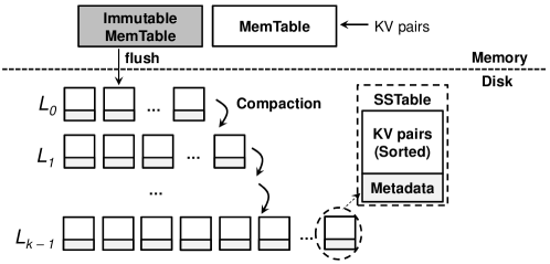
Figure 1: Data organization in LevelDB.

If $L_{0}$ is full, LevelDB flushes and merges the KV pairs in $L_{0}$ into $L_{1}$ via compaction; similarly, if $L_{1}$ is full, LevelDB flushes and merges the KV pairs in $L_{1}$ into $L_{2}$, and so on. The compaction process comprises three steps. First, it reads out KV pairs in both $L_{i}$ and $L_{i+1}$ into memory (where $i\geq 0$). Second, it sorts the valid KV pairs (i.e., the KV pairs that are newly inserted or updated) by keys and reorganizes them into SSTables. It also discards all invalid KV pairs (i.e., the KV pairs that are deleted or superseded by new updates). Finally, it writes back all SSTables with valid KV pairs to $L_{i+1}$. Note that all KV pairs in each level, except $L_{0}$, are sorted by keys. In $L_{0}$, LevelDB only keeps KV pairs sorted within each SSTable, but not across SSTables. This improves performance of flushing KV pairs from the MemTable to disk.

To perform a key lookup, LevelDB searches from $L_{0}$ to $L_{k-1}$ and returns the first associated value found. In $L_{0}$, LevelDB searches all SSTables. In each level between $L_{1}$ and $L_{k-1}$, LevelDB first identifies a candidate SSTable and checks its Bloom filter to determine if the KV pair exists. If so, LevelDB reads the candidate SSTable and searches for the KV pair; otherwise, it directly searches the lower levels.

Limitations:

LevelDB achieves high random write performance via the LSM-tree-based design, but suffers from both write and read amplifications. First, the compaction process inevitably incurs extra reads and writes. In the worst case, to merge one SSTable from $L_{i-1}$ to $L_{i}$, it reads and sorts 10 SSTables, and writes back all SSTables. Prior studies show that LevelDB can have an overall write amplification of at least 50$\times$ [49, 28], since it may trigger more than one compaction to move a KV pair down multiple levels under large workloads.

Also, a lookup operation may search multiple levels for a KV pair and incur multiple disk accesses. The reason is that the search in each level needs to read the indexing metadata and the Bloom filter in the associated SSTable. Although the Bloom filter is used, it may introduce false positives. In this case, a lookup may still unnecessarily read an SSTable from disk even though the KV pair actually does not exist in the SSTable. Thus, each lookup typically incurs multiple disk accesses. Such read amplification further aggravates under large workloads, as the LSM-tree builds up in levels. Measurements show that the read amplification can reach over 300$\times$ in the worst case [28].

2.2 KV Separation

KV separation, proposed by WiscKey [28], decouples the management of keys and values to mitigate both write and read amplifications. The rationale is that storing values in the LSM-tree is unnecessary for indexing. Thus, WiscKey stores only keys and metadata (e.g., key/value sizes, value locations, etc.) in the LSM-tree, while storing values in a separate append-only circular log called vLog. KV separation effectively mitigates write and read amplifications of LevelDB as it significantly reduces the size of the LSM-tree, and hence both compaction and lookup overheads.

Since vLog follows the log-structured design [40], it is critical for KV separation to achieve lightweight garbage collection (GC) in vLog, i.e., to reclaim the free space from invalid values with limited overhead. Specifically, WiscKey tracks the vLog head and the vLog tail, which correspond to the end and the beginning of vLog, respectively. It always inserts new values to the vLog head. When it performs a GC operation, it reads a chunk of KV pairs from the vLog tail. It first queries the LSM-tree to see if each KV pair is valid. It then discards the values of invalid KV pairs, and writes back the valid values to the vLog head. It finally updates the LSM-tree for the latest locations of the valid values. To support efficient LSM-tree queries during GC, WiscKey also stores the associated key and metadata together with the value in vLog. Note that vLog is often over-provisioned with extra reserved space to mitigate GC overhead.

Limitations:

While KV separation reduces compaction and lookup overheads, we argue that it suffers from the substantial GC overhead in vLog. Also, the GC overhead becomes more severe if the reserved space is limited. The reasons are two-fold.

First, vLog can only reclaim space from its vLog tail due to its circular log design. This constraint may incur unnecessary data movements. In particular, real-world KV storage often exhibits strong locality [2], in which a small portion of hot KV pairs are frequently updated, while the remaining cold KV pairs receive only few or even no updates. Maintaining a strict sequential order in vLog inevitably relocates cold KV pairs many times and increases GC overhead.

Also, each GC operation queries the LSM-tree to check the validity of each KV pair in the chunk at the vLog tail. Since the keys of the KV pairs may be scattered across the entire LSM-tree, the query overhead is high and increases the latency of the GC operation. Even though KV separation has already reduced the size of the LSM-tree, the LSM-tree is still sizable under large workloads, and this aggravates the query cost.

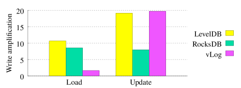
Figure 2: Write amplifications of LevelDB, RocksDB, and vLog in the load and update phases.

To validate the limitations of KV separation, we implement a KV store prototype based on vLog (§3.8) and evaluate its write amplification. We consider two phases: load and update. In the load phase, we insert 40 GiB of 1-KiB KV pairs into vLog that is initially empty. Each KV pair comprises 8-B metadata (including the key/value size fields and reserved information), a 24-B key, and a 992-B value. We insert the KV pairs based on the default hashed order in YCSB [8], such that the keys are the hashed outputs of some seed numbers; in other words, the keys of the inserted KV pairs appear in random order. In the update phase, we generate skewed access patterns (as observed in real-world KV storage workloads [2]); specifically, we issue 40 GiB of updates to the existing KV pairs based on a heavy-tailed Zipf distribution with a Zipfian constant of 0.99 (the default Zipfian constant in YCSB [8]). We provision 40 GiB of space for vLog, and an additional 30% (i.e., 12 GiB) of reserved space. We also disable the write cache in our prototype (§3.2). Figure 2 shows the write amplification results of vLog in the load and update phases, in terms of the ratio of the total device write size to the actual write size due to inserts or updates. For comparison, we also consider two modern KV stores, LevelDB [18] and RocksDB [14], based on their default parameters. In the load phase, vLog has sufficient space to hold all KV pairs and does not trigger GC, so its write amplification is only 1.6$\times$ due to KV separation. However, in the update phase, the updates fill up the reserved space and start to trigger GC. We see that vLog has a write amplification of 19.7$\times$, which is close to LevelDB (19.1$\times$) and higher than RocksDB (7.9$\times$).

To mitigate GC overhead in vLog, one approach is to partition vLog into segments and choose the best candidate segments for GC (e.g., based on the cost-benefit policy or its variants [40, 32, 41]). However, the hot and cold KV pairs can still be mixed together in vLog, so the chosen segments for GC may still contain cold KV pairs that are unnecessarily moved.

To address the mixture of hot and cold data, a better approach is to perform hot-cold data grouping as in SSD designs [33, 23], in which we separate the storage of hot and cold KV pairs into two regions and apply GC to each region individually (more GC operations are expected to be applied to the storage region for hot KV pairs). However, the direct implementation of hot-cold data grouping inevitably increases the update latency in KV separation. As a KV pair may be stored in either hot or cold regions, each update needs to first query the LSM-tree for the exact storage location of the KV pair. Thus, a key motivation of our work is to enable hotness awareness without LSM-tree lookups.

3 HashKV Design

HashKV is a persistent KV store that specifically targets update-intensive workloads. It improves the management of value storage atop KV separation to achieve high update performance. It supports standard KV operations: PUT (i.e., writing a KV pair), GET (i.e., retrieving the value of a key), DELETE (i.e., deleting a KV pair), and SCAN (i.e., retrieving the values of a range of keys).

3.1 Main Idea

HashKV follows KV separation [28] by storing only keys and metadata in the LSM-tree for indexing KV pairs, while storing values in a separate area called the value store. Atop KV separation, HashKV introduces several core design elements to achieve efficient value storage management.

• Hash-based data grouping: Recall that vLog incurs substantial GC overhead in value storage. Instead, HashKV maps values into fixed-size partitions in the value store by hashing the associated keys. This design achieves: (i) partition isolation, in which all versions of value updates associated with the same key must be written to the same partition, and (ii) deterministic grouping, in which the partition where a value should be stored is determined by hashing. We leverage this design to achieve flexible and lightweight GC.

• Dynamic reserved space allocation: Since we map values into fixed-size partitions, one challenge is that a partition may receive more updates than it can hold. HashKV allows a partition to grow dynamically beyond its size limit by allocating fractions of reserved space in the value store to hold the extra updates.

• Hotness awareness: Due to deterministic grouping, a partition may be filled with the values from a mix of hot and cold KV pairs, in which case a GC operation unnecessarily reads and writes back the values of cold KV pairs. HashKV uses a tagging approach to relocate the values of cold KV pairs to a different storage area and separate the hot and cold KV pairs, so that we can apply GC to hot KV pairs only and avoid re-copying cold KV pairs.

• Selective KV separation: HashKV differentiates KV pairs by their value sizes, such that the small-size KV pairs can be directly stored in the LSM-tree without KV separation. This saves the overhead of accessing both the LSM-tree and the value store for small-size KV pairs, while the compaction overhead of storing the small-size KV pairs in the LSM-tree is limited.

Remarks: HashKV maintains a single LSM-tree for indexing (instead of hash-partitioning the LSM-tree as in the value store) to preserve the ordering of keys and the range scan performance. Since hash-based data grouping spreads KV pairs across the value store, it incurs random writes; in contrast, vLog maintains sequential writes with a log-structured storage layout. Our HashKV prototype (§3.8) exploits both multi-threading and batch writes to limit random write overhead.

3.2 Storage Management

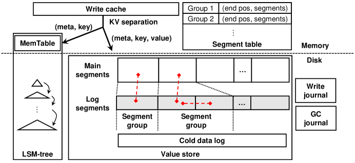
Figure 3: HashKV architecture. Each segment group consists of one main segment and a variable number (zero or more) of log segments; the log segments (in shaded color) are provisioned in reserved space. For example, the segments that are linked together belong to the same segment group.

Figure 3 depicts the architecture of HashKV. It divides the logical address space of the value store into fixed-size units called main segments. Also, it over-provisions a fixed portion of reserved space, which is again divided into fixed-size units called log segments. Note that the sizes of main segments and log segments are configurable and may differ; by default, we set them as 64 MiB and 1 MiB, respectively.

For each insert or update of a KV pair, HashKV hashes its key into one of the main segments. If the main segment is not full, HashKV stores the value in a log-structured manner by appending the value to the end of the main segment; on the other hand, if the main segment is full, HashKV dynamically allocates a free log segment to store the extra values in a log-structured manner. Again, it further allocates additional free log segments if the current log segment is full. We collectively call a main segment and all its associated log segments (if any) a segment group, as shown in Figure 3. Also, HashKV updates the LSM-tree for the latest value location. To keep track of the storage status of the segment groups and segments, HashKV uses a global in-memory segment table to store the current end position of each segment group for subsequent inserts or updates, as well as the list of log segments associated with each segment group. Our design ensures that each insert or update can be directly mapped to the correct write position without issuing LSM-tree lookups on the write path, thereby achieving high write performance. Also, the updates of the values associated with the same key must go to the same segment group, and this simplifies GC. For fault tolerance, HashKV checkpoints the segment table to persistent storage.

To facilitate GC, HashKV also stores the key and metadata (e.g., key/value sizes) together with the value for each KV pair in the value store as in WiscKey [28] (Figure 3). This enables a GC operation to quickly identify the key associated with a value when it scans the value store. However, our GC design inherently differs from vLog used by WiscKey (§3.3).

To improve write performance, HashKV holds an in-memory write cache to store the recently written KV pairs, at the expense of degrading reliability. If the key of a new KV pair to be written is found in the write cache, HashKV directly updates the value of the cached key in-place without issuing the writes to the LSM-tree and the value store. It can also return the KV pairs from the write cache for reads. If the write cache is full, HashKV flushes all the cached KV pairs to the LSM-tree and the value store. Note that the write cache is an optional component and can be disabled for reliability concerns.

HashKV supports hotness awareness by keeping cold values in a separate cold data log (§3.4). It also addresses crash consistency by tracking the updates in both write journal and GC journal (§3.7). Note that the sizes of the cold data log and the journals are configurable.

3.3 Garbage Collection (GC)

HashKV necessitates GC to reclaim the space occupied by invalid KV pairs in the value store. In HashKV, GC operates in units of segment groups, and is triggered when the free log segments in the reserved space are running out. At a high level, a GC operation first selects a candidate segment group and identifies all valid KV pairs in the group. It then writes back all valid KV pairs to the main segment, or additional log segments if needed, in a log-structured manner. It also releases any unused log segments that can be later used by other segment groups. Finally, it updates the latest value locations in the LSM-tree. Here, the GC operation needs to address two issues: (i) which segment group should be selected for GC; and (ii) how the GC operation quickly identifies the valid KV pairs in the selected segment group.

Unlike vLog, which requires the GC operation to follow a strict sequential order, HashKV can flexibly choose which segment group to perform GC. By default, it adopts a greedy approach and selects the segment group with the largest amount of writes. The rationale is that the selected segment group typically holds the hot KV pairs that have many updates and hence has a large amount of writes. Thus, selecting this segment group for GC likely reclaims the most free space. To realize the greedy approach, HashKV tracks the amount of writes for each segment group in the in-memory segment table (§3.2), and uses a heap to quickly identify which segment group receives the largest amount of writes.

HashKV can adopt other approaches of choosing a segment group for GC. We implement two additional approaches, namely the cost-benefit algorithm (CBA) [41] and the greedy random algorithm (GRA) [24]. CBA takes into account both the age of a segment group (the time since its last GC operation) and the fraction of valid data in the segment group when determining which segment group is chosen for GC. Intuitively, CBA prefers to choose a segment group with a larger age (i.e., it is more stable) and a lower fraction of valid data (i.e., it has more free space reclaimed) for GC. GRA mixes both the greedy and random approaches, such that it first selects the top-$d$ segment groups that receive the largest amounts of writes for some configurable parameter $d$, followed by randomly selecting a segment group among the top-$d$ ones. Note that when $d=1$, GRA reduces to the greedy approach; when $d$ is at least the total number of segment groups, GRA reduces to the random approach.

To check the validity of KV pairs in the selected segment group, HashKV sequentially scans the KV pairs in the segment group without querying the LSM-tree (note that it also checks the write cache for any latest KV pairs in the segment group). Since HashKV writes the KV pairs to the segment group in a log-structured manner, the KV pairs must be sequentially placed according to their order of being updated. For a KV pair that has multiple versions of updates, the version that is nearest to the end of the segment group must be the latest one and correspond to the valid KV pair, while other versions are invalid. Thus, the running time for each GC operation only depends on the size of the segment group that needs to be scanned. In contrast, the GC operation in vLog reads a chunk of KV pairs from the vLog tail (§2.2). It queries the LSM-tree (based on the keys stored along with the values) for the latest storage location of each KV pair in order to check if the KV pair is valid [28]. The overhead of querying the LSM-tree becomes substantial under large workloads.

During a GC operation on a segment group, HashKV constructs a temporary in-memory hash table (indexed by keys) to buffer the addresses of the valid KV pairs being found in the segment group. As the key and address sizes are generally small and the number of KV pairs in a segment group is limited, the hash table has limited size and can be entirely stored in memory. HashKV blocks incoming writes during a GC operation, so that KV pairs remain intact when being relocated to different segments.

3.4 Hotness Awareness

Hot-cold data separation improves GC performance in log-structured storage (e.g., SSDs [33, 23]). In fact, the current hash-based data grouping design realizes some form of hot-cold data separation, since the updates of the hot KV pairs must be hashed to the same segment group and our current GC policy always chooses the segment group that is likely to store the hot KV pairs (§3.3). However, it is inevitable that some cold KV pairs are hashed to the segment group selected for GC, leading to unnecessary data rewrites. Thus, a challenge is to fully realize hot-cold data separation to further improve GC performance.

HashKV relaxes the restriction of hash-based data grouping via a tagging approach (Figure 4). Specifically, when HashKV performs a GC operation on a segment group, it classifies each KV pair in the segment group as hot or cold. Currently, we treat the KV pairs that are updated at least once since their last inserts as hot, or cold otherwise (more accurate hot-cold data identification approaches [20] can be used). For the hot KV pairs, HashKV still writes back their latest versions to the same segment group via hashing. However, for the cold KV pairs, it now writes their values to a separate storage area, and keeps their key and metadata only (i.e., without values) in the segment group. In addition, it adds a tag in the metadata of each cold KV pair to indicate its presence in the segment group. Thus, if a cold KV pair is not updated, a GC operation only rewrites its key and metadata without rewriting its value, thereby saving the rewrite overhead. On the other hand, if a cold KV pair is later updated, we know directly from the tag (without querying the LSM-tree) that the cold KV pair has already been stored, so that we can treat it as hot based on our classification policy; also, the tagged KV pair will become invalid and can be reclaimed in the next GC operation. Finally, at the end of a GC operation, HashKV updates the latest value locations in the LSM-tree, such that the locations of the cold KV pairs point to the separate storage area.

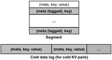
Figure 4: Tagging in HashKV. Note that the locations of the cold KV pairs in the cold data log are stored in the LSM-tree.

With tagging, HashKV avoids storing the values of cold KV pairs in the segment group and rewriting them during GC. Also, tagging is only triggered during GC, and does not add extra overhead to the write path. Currently, we implement the separate storage area for cold KV pairs as an append-only log (called the cold data log) in the value store, and perform GC on the cold data log as in vLog. The cold data log can also be put in secondary storage with a larger capacity (e.g., hard disks) if the cold KV pairs are rarely accessed.

3.5 Selective KV Separation

HashKV supports workloads with general value sizes. Our rationale is that KV separation reduces compaction overhead especially for large-size KV pairs, yet its benefits for small-size KV pairs are limited, and it incurs extra overhead of accessing both the LSM-tree and the value store. Thus, we propose selective KV separation, in which we still apply KV separation to KV pairs with large value sizes, while storing KV pairs with small value sizes in entirety in the LSM-tree. A key challenge of selective KV separation is to choose the KV pair size threshold of differentiating between small-size and large-size KV pairs (assuming that the key size remains fixed).

Here, we propose a simple search method to choose the appropriate threshold. Our idea is to benchmark the update performance of different KV pair sizes with and without KV separation on the platform where we deploy HashKV. As a case study, we conduct performance benchmarking based on our testbed (§4.1) and update-intensive workloads (§4.2). We first load 40 GiB of KV pairs into HashKV, which is initially empty. We then repeatedly issue three phases of 40 GiB updates to obtain a stable update throughput. If KV separation is disabled, all updates are directly stored in LevelDB (on which HashKV manages keys and metadata); otherwise if KV separation is enabled, we allocate 30% of reserved space to HashKV for value management. Figure 5 shows the update throughput for the last phase of 40 GiB updates versus the KV pair size; here, we fix the key size as 24 B and the metadata size as 8 B. When the KV pair size is small, the overhead of accessing both the LSM-tree and the value store in KV separation is significant, so enabling KV separation has worse performance. When the KV pair size increases, KV separation improves performance, and it shows performance gains when the KV pair size is between 128 B and 192 B. Thus, we choose 192 B as our default threshold for selective KV separation. Interestingly, even though we choose our threshold based on update-intensive workloads, our search method is fairly robust and the threshold also works well for other types of workloads (see §4.5 for details).

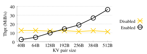
Figure 5: Update throughput versus the KV pair size with and without KV separation.

3.6 Range Scans

One critical reason of using the LSM-tree for indexing is its efficient support of range scans. Since the LSM-tree stores and sorts KV pairs by keys, it can return the values of a range of keys via sequential reads. However, KV separation now stores values in separate storage space, so it incurs extra reads of values. In HashKV, the values are scattered across different segment groups, so range scans will trigger many random reads that degrade performance. HashKV currently leverages the read-ahead mechanism to speed up range scans by prefetching values into the page cache. For each scan request, HashKV iterates over the range of sorted keys in the LSM-tree, and issues a read-ahead request to each value (via posix_fadvise). It then reads all values and returns the sorted KV pairs. Note that Wisckey [28] fetches values in the background while iterating over keys.

3.7 Crash Consistency

Crashes can occur while HashKV issues writes to persistent storage. HashKV addresses crash consistency based on metadata journaling and focuses on two aspects: (i) flushing the write cache and (ii) GC operations.

Flushing the write cache involves writing the KV pairs to the value store and updating metadata in the LSM-tree. HashKV maintains a write journal to track each flushing operation. It performs the following steps when flushing the write cache: (i) flushing the cached KV pairs to the value store; (ii) appending metadata updates to the write journal; (iii) writing a commit record to the journal end; (iv) updating keys and metadata in the LSM-tree; and (v) marking the flush operation free in the journal (the freed journaling records can be recycled later). If a crash occurs after step (iii) completes, HashKV replays the updates in the write journal and ensures that the LSM-tree and the value store are consistent.

Handling crash consistency in GC operations is different, as they may overwrite existing valid KV pairs. Thus, we also need to protect existing valid KV pairs against crashes during GC. HashKV maintains a GC journal to track each GC operation. It performs the following steps after identifying all valid KV pairs during a GC operation: (i) appending the valid KV pairs that are overwritten as well as metadata updates to the GC journal; (ii) writing all valid KV pairs back to the segment group; (iii) updating the metadata in the LSM-tree; and (iv) marking the GC operation free in the journal.

3.8 Implementation Details

We prototype HashKV in C++ on Linux. For key and metadata management, HashKV uses LevelDB v1.20 [18] by default, yet it can also leverage other LSM-tree-based KV stores to improve their respective performance (§4.5). Our prototype contains around 6.7K lines of code (without LevelDB).

Storage organization:

We currently deploy HashKV on the Linux Ext4 file system, on which we run both LevelDB and the value store. In particular, HashKV manages the value store as a large file. It partitions the value store file into two regions, one for main segments and another for log segments, according to the pre-configured segment sizes. All segments are aligned in the value store file, such that the start offset of each main (resp. log) segment is a multiple of the main (resp. log) segment size. If hotness awareness is enabled (§3.4), HashKV adds a separate region in the value store file for the cold data log. Also, to address crash consistency (§3.7), HashKV uses separate files to store both write and GC journals.

Multi-threading:

HashKV implements multi-threading via threadpool [46] to boost I/O performance when flushing KV pairs in the write cache to different segments (§3.2) and retrieving segments from segment groups in parallel during GC (§3.3).

To mitigate random write overhead due to deterministic grouping (§3.1), HashKV implements batch writes. When HashKV flushes KV pairs in the write cache, it first identifies and buffers a number of KV pairs that are hashed to the same segment group in a batch, and then issues a sequential write (via a thread) to flush the batch. A larger batch size reduces random write overhead, yet it also degrades parallelism. Currently, we configure a batch write threshold, such that after adding a KV pair into a batch, if the batch size reaches or exceeds the batch size threshold, the batch will be flushed; in other words, HashKV directly flushes a KV pair if its size is larger than the batch write threshold. Note that WiscKey [28] also uses a write buffer to batch KV pairs into sequential writes. HashKV further issues parallel writes via multi-threading using a configurable batch size threshold.

4 Evaluation

We compare via testbed experiments HashKV with several state-of-the-art KV stores: LevelDB (v1.20) [18], RocksDB (v5.8) [14], HyperLevelDB [13], PebblesDB [38], and our own vLog implementation for KV separation based on WiscKey [28]. Note that BadgerDB [12] is an open-source implementation of KV separation based on WiscKey and is written in Golang. However, it currently supports manual compaction only, and we do not include BadgerDB in our evaluation.

For fair comparison, we build a unified framework to integrate each state-of-the-art KV store and HashKV. Specifically, we buffer all written KV pairs in the write cache and flush them when the write cache is full. For LevelDB, RocksDB, HyperLevelDB, and PebblesDB, we flush all KV pairs in entirety to them; for vLog and HashKV, we flush keys and metadata to LevelDB, and values (together with keys and metadata) to the value store. We address the following questions:

• How is the update performance of HashKV compared to other KV stores under update-intensive workloads? (Experiment 1)

• How do the reserved space size and RAID configurations affect the update performance of HashKV? (Experiments 2 and 3)

• What is the performance of HashKV in updates and range scans for different KV pair sizes? (Experiments 4 and 5)

• What are the performance gains of hotness awareness and selective KV separation? (Experiments 6 and 7)

• How do different KV pair size thresholds affect the performance gains of selective KV separation? (Experiment 8)

• How do different GC approaches affect the update performance of HashKV? (Experiment 9)

• How does the crash consistency mechanism affect the update performance of HashKV? (Experiment 10)

• What is the performance of HashKV compared to other KV stores under YCSB core workloads? (Experiments 11 and 12)

• What is the performance of HashKV when it builds on other KV stores? (Experiment 13)

• What is the storage distribution of the value store of HashKV? (Experiment 14)

• How do parameter configurations (e.g., main segment size, log segment size, and write cache size) affect the update performance of HashKV? (Experiment 15)

4.1 Setup

Testbed: We conduct our experiments on a machine running Ubuntu 14.04 LTS with Linux kernel 3.13.0. The machine is equipped with a quad-core Xeon E3-1240v2, 16 GiB RAM, and seven Plextor M5 Pro 128 GiB SSDs. One SSD is attached to the motherboard as the OS drive, while the remaining six SSDs are attached to the LSI SAS 9201-16i host bus adapter to form an SSD RAID volume for high I/O performance. Specifically, we create a software RAID volume using mdadm [27] atop the six SSDs, with a chunk size of 4 KiB. We run each KV store on the SSD RAID volume.

Default setup:

For LevelDB, RocksDB, HyperLevelDB, and PebblesDB, we use their default parameters. We allow them to use all available capacity in our SSD RAID volume, so that their major overheads come from read and write amplifications in the LSM-tree management.

For vLog, we configure it to read 64 MiB from the vLog tail (§2.2) in each GC operation. For HashKV, we set the main segment size as 64 MiB and the log segment size as 1 MiB. Both vLog and HashKV are configured with 40 GiB of storage space and over-provisioned with 30% (i.e., 12 GiB) of reserved space, while their key and metadata storage in LevelDB can use all available storage space. Also, we do not limit the sizes of the cold data log and the journals. Here, we provision the storage space of vLog and HashKV to be close to the actual KV store sizes of LevelDB and RocksDB based on our evaluation (Experiment 1).

We mount the SSD RAID volume under RAID-0 (no fault tolerance) by default to maximize performance. All KV stores run in asynchronous mode and are equipped with a write cache of size 64 MiB. For HashKV, we set the batch write threshold (§3.8) to 4 KiB, and configure 32 and 8 threads for write cache flushing and segment retrieval in GC, respectively. We disable selective KV separation, hotness awareness, and crash consistency in HashKV by default, except when we evaluate them.

4.2 Performance Comparison

We compare the performance of different KV stores under update-intensive workloads. Specifically, we generate workloads using YCSB [8], and fix the size of each KV pair as 1 KiB, which consists of 8-B metadata (including the key/value size fields and reserved information), a 24-B key, and a 992-B value. We assume that each KV store is initially empty. We first load 40 GiB of KV pairs (or 42 M inserts) into each KV store (call it Phase P0). We then repeatedly issue 40 GiB of updates over the existing 40 GiB of KV pairs three times (call them Phases P1, P2, and P3), accounting for 120 GiB or 126 M updates in total. Updates in each phase follow a heavy-tailed Zipf distribution with a Zipfian constant of 0.99. We issue the requests to each KV store as fast as possible to stress-test its performance.

Note that vLog and HashKV do not trigger GC in Phase P0. In Phase P1, when the reserved space becomes full after 12 GiB of updates, both systems start to trigger GC; in both Phases P2 and P3, updates are issued to the fully filled value store and will trigger GC frequently. We include both Phases P2 and P3 to ensure that the update performance is stable.

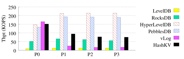
(a) Throughput (load phase: P0, update phases: P1 - P3)
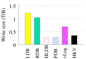
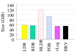
(b) Total write size	(c) KV store size
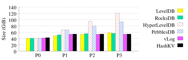
(d) KV store size at the end of each phase
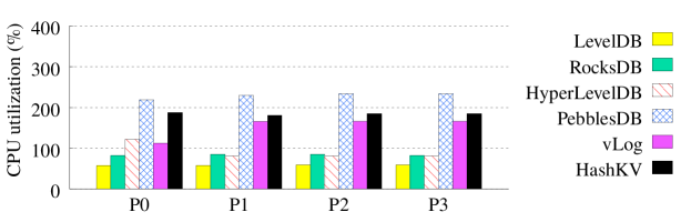
(e) CPU utilization

Figure 6: Experiment 1: Performance comparison of KV stores under update-intensive workloads.

Experiment 1 (Load and update performance):

We evaluate LevelDB (LDB), RocksDB (RDB), HyperLevelDB (HDB), PebblesDB (PDB), vLog, and HashKV (HKV), under update-intensive workloads. We first compare LevelDB, RocksDB, vLog, and HashKV; later, we also include HyperLevelDB and PebblesDB into our comparison.

Figure 6(a) shows the performance of each phase. For vLog and HashKV, the throughput in the load phase is higher than those in the update phases, as the latter is dominated by the GC overhead. In the load phase, the throughput of HashKV is 17.1$\times$ and 3.0$\times$ over LevelDB and RocksDB, respectively. HashKV’s throughput is 7.9% slower than vLog, due to random writes introduced to distribute KV pairs via hashing. In the update phases, the throughput of HashKV is 6.3-7.9$\times$, 1.3-1.4$\times$, and 3.7-4.6$\times$ over LevelDB, RocksDB, and vLog, respectively. LevelDB has the lowest throughput among all KV stores due to significant compaction overhead, while vLog also suffers from high GC overhead.

Figures 6(b) and 6(c) show the total write sizes and the KV store sizes of different KV stores after all load and update requests are issued. HashKV reduces the total write sizes of LevelDB, RocksDB and vLog by 71.5%, 66.7%, and 49.6%, respectively. Also, they have very similar KV store sizes.

For HyperLevelDB and PebblesDB, both of them have high load and update throughput due to their low compaction overhead. For example, PebblesDB appends fragmented SSTables from the higher level to the lower level, without rewriting SSTables at the lower level [38]. Both HyperLevelDB and PebblesDB achieve at least 2$\times$ throughput of HashKV, while incurring lower write sizes than HashKV. On the other hand, they incur significant storage overhead, and their final KV store sizes are 2.2$\times$ and 1.7$\times$ over HashKV, respectively.

We further analyze the storage overhead of LevelDB, RocksDB, HyperLevelDB, PebblesDB, vLog, and HashKV under update-intensive workloads. In particular, we elaborate the reasons on the significant storage overhead observed in HyperLevelDB and PebblesDB.

Figure 6(d) shows the KV store size of each KV store at the end of each phase. At the end of the load phase (Phase P0), the sizes of all KV stores only differ by at most 4.6%; in particular, the differences of the KV store sizes among LevelDB, RocksDB, HyperLevelDB, and PebblesDB are only at most 1.17%, which aligns with the space amplification results under the insertion-only workload in [38]. Both vLog and HashKV have slightly larger KV store sizes than others, mainly because the keys and metadata are stored in both the LSM-tree and the value store due to KV separation (§3.2). From Phase P0 to Phase P3, the KV store sizes of LevelDB, RocksDB, vLog, and HashKV increase by 42.1%, 38.9%, 28.9%, and 27.0%, respectively, while the KV store sizes of HyperLevelDB and PebblesDB increase significantly and are 3.0$\times$ and 2.3$\times$ their sizes at the end of Phase P0, respectively.

The reasons of the significant increase in the KV store sizes of HyperLevelDB and PebblesDB are two-fold. First, both HyperLevelDB and PebblesDB compact only selected ranges of keys to reduce write amplification. Specifically, HyperLevelDB selects the largest range of keys in the upper level that covers the smallest range of keys in the lower level to perform compaction, and places a limit on the total volume of KV pairs in each compaction. This reduces the amount of invalid KV pairs being reclaimed from the lower level during compaction. PebblesDB divides keys in each level into disjoint ranges and compacts each range only when its size reaches a predefined threshold. To enable fast compaction, PebblesDB only partitions KV pairs in the selected ranges and directly inserts them into the lower level, without removing invalid KV pairs in the lower level. This also reduces the amount of invalid KV pairs being reclaimed.

Second, HyperLevelDB and PebblesDB trigger much fewer compaction operations under the update-intensive workloads; for example, their numbers of compaction operations are only 1.6% and 0.02% of that of LevelDB, respectively. Such infrequent compaction operations further delay the removal of invalid KV pairs and hence lead to large KV store sizes.

We emphasize that this experiment only shows the baseline performance of HashKV rather than its best performance. For example, if we allocate more reserved space (Experiment 2) and issue larger-size KV pairs (Experiment 4), HashKV achieves higher throughput. Also, we can improve the performance of HashKV by enabling hotness awareness (Experiment 6) and selective KV separation (Experiment 7). Furthermore, HashKV outperforms HyperLevelDB and PebblesDB under the YCSB core workloads (Experiment 11). In the following experiments, except YCSB benchmarking and the impact of KV separation on different KV stores, we mainly focus on LevelDB, RocksDB, vLog, and HashKV, as they have comparable storage overhead.

Finally, Figure 6(e) shows the CPU utilization of each KV store in different phases. Here, we sample the CPU utilization (in percentage) of each KV store every one second using nmon [19], and plot the median CPU usage. Since the CPU has four cores, the maximum achievable CPU utilization is 400%. We observe that in the load phase (Phase P0), HashKV has 75% higher CPU utilization than vLog. Our further investigation finds that the high CPU utilization of HashKV is attributed to the flushing of KV pairs from the write cache to different segments. In the update phases, vLog has higher CPU utilization than in its load phase, as its GC overhead now becomes significant. In contrast, HashKV maintains similar CPU utilization in both load and update phases, and its CPU utilization is 15-18% higher than vLog in each update phase. PebblesDB has the highest CPU utilization in all phases due to more aggressive compaction, as also reported in [38].

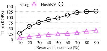
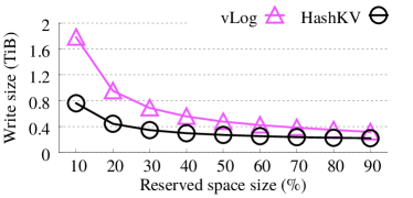
(a) Throughput	(b) Total write size
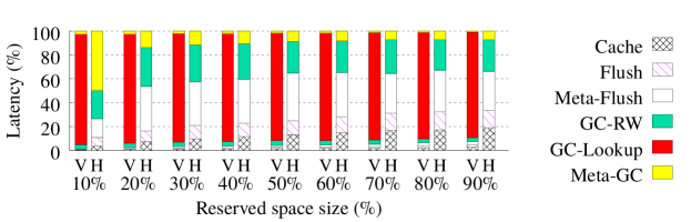
(c) Latency breakdown (‘V’$=$ vLog; ‘H’$=$ HashKV)

Figure 7: Experiment 2: Impact of reserved space size.

Experiment 2 (Impact of reserved space):

We study the impact of reserved space size on the update performance of vLog and HashKV. We vary the reserved space size from 10% to 90% (of 40 GiB). Figure 7 shows the performance in Phase P3, including the update throughput, the total write size, and the latency breakdown. Both vLog and HashKV benefit from the increase in reserved space. Nevertheless, HashKV achieves 3.1-4.7$\times$ throughput of vLog (Figure 7(a)) and reduces the write size of vLog by 30.1-57.3% (Figure 7(b)) across different reserved space sizes.

We further analyze the latency breakdown of the update requests in Phase P3 for vLog and HashKV (Figure 7(c)). The breakdown includes the fractions of time spent on the major steps in an update request, including: processing the write cache (“Cache”), flushing values from the write cache (“Flush”), updating metadata in the LSM-tree during flush (“Meta-Flush”), reading and writing values during GC (“GC-RW”), querying the LSM-tree during GC (“GC-Lookup”), and updating metadata in the LSM-tree during GC (“Meta-GC”). We see that the high GC overhead of vLog is mainly attributed to the queries of the LSM-tree for checking the validity of KV pairs (i.e., “GC-Lookup”), and such queries account for over 80% of the overall update latency. On the other hand, HashKV eliminates this LSM-tree query overhead in GC. Furthermore, we observe that HashKV spends less time on updating metadata during GC (i.e., “Meta-GC”) in the LSM-tree with the increasing reserved space size due to less frequent GC operations.

Reserved space size	10%	20%	30%	40%	50%	60%	70%	80%	90%
vLog	160.70	81.17	57.57	46.19	40.60	38.04	32.86	27.72	24.46
HashKV	36.21	17.05	13.07	11.07	10.25	8.99	8.14	7.83	7.72

Table 1: Experiment 2: Average update latencies (in microseconds) of vLog and HashKV.

Table 1 shows the average update latencies of vLog and HashKV in Phase P3. The update latencies of both vLog and HashKV decrease when the reserved space size increases, due to less frequent GC operations. The update latency of HashKV is generally lower than that of vLog for different reserved space sizes.

Experiment 3 (Impact of parity-based RAID):

We evaluate the impact of the fault tolerance configuration of RAID on the update performance of LevelDB, RocksDB, vLog, and HashKV. We configure the RAID volume to run two parity-based RAID schemes, RAID-5 (single-device fault tolerance) and RAID-6 (double-device fault tolerance). We include the results under RAID-0 for comparison. Figure 8 shows the throughput in Phase P3 and the total write size. RocksDB and HashKV are more sensitive to RAID configurations (larger drops in throughput), since their performance is write-dominated. Nevertheless, the throughput of HashKV is higher than other KV stores under parity-based RAID schemes, e.g., 4.8$\times$, 3.2$\times$, and 2.7$\times$ over LevelDB, RocksDB, and vLog, respectively, under RAID-6. The write sizes of KV stores under RAID-5 and RAID-6 increase by around 20% and 50%, respectively, compared to RAID-0, which match the amount of redundancy of the corresponding parity-based RAID schemes.

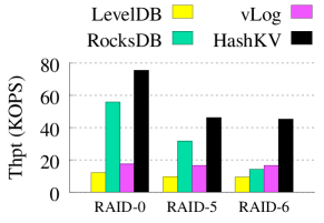
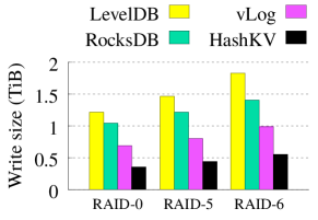
(a) Throughput	(b) Total write size

Figure 8: Experiment 3: Different RAID configurations.

4.3 Performance under Different Workloads

We now study the update and range scan performance of HashKV for different KV pair sizes.

Experiment 4 (Impact of KV pair size):

We study the impact of KV pair sizes on the update performance of KV stores. We vary the KV pair size from 256 B to 64 KiB. Specifically, we increase the KV pair size by increasing the value size and keeping the key size fixed at 24 B. We also reduce the number of KV pairs loaded or updated, so as to keep the total size of KV pairs fixed at 40 GiB. Figure 9 shows the update performance of KV stores in Phase P3 versus the KV pair size. The throughput of LevelDB and RocksDB remains similar across most KV pair sizes, while the throughput of vLog and HashKV increases as the KV pair size increases. Both vLog and HashKV have lower throughput than RocksDB when the KV pair size is 256 B, since the overhead of writing small values to the value store is more significant. Nevertheless, HashKV can benefit from selective KV separation (Experiment 7). As the KV pair size increases, HashKV also sees increasing throughput. For example, HashKV achieves 15.5$\times$ and 2.8$\times$ throughput over LevelDB and RocksDB, respectively, for 4-KiB KV pairs. HashKV achieves 2.2-5.1$\times$ throughput over vLog for KV pair sizes between 256 B and 4 KiB. The performance gap between vLog and HashKV narrows as the KV pair size increases, since the size of the LSM-tree decreases with fewer KV pairs. Thus, the queries to the LSM-tree of vLog are less expensive. For 64-KiB KV pairs, HashKV has 10.7% less throughput than vLog.

When the KV pair size increases, the total write sizes of LevelDB and RocksDB increase due to the increasing compaction overhead, while those of HashKV and vLog decrease due to fewer KV pairs in the LSM-tree. Overall, HashKV reduces the total write sizes of LevelDB, RocksDB, and vLog by 43.2-78.8%, 33.8-73.5%, and 3.5-70.6%, respectively.

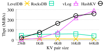
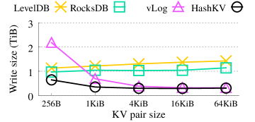
(a) Throughput	(b) Total write size

Figure 9: Experiment 4: Update performance versus the KV pair size.

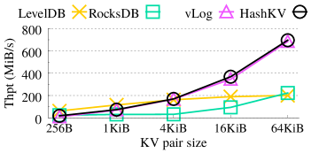
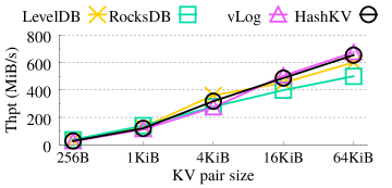
(a) After the load phase	(b) After the update phases

Figure 10: Experiment 5: Range scan performance versus the KV pair size.

Experiment 5 (Range scans):

We compare the range scan performance of KV stores for different KV pair sizes. Specifically, we first load 40 GiB of fixed-size KV pairs, and then issue scan requests whose start keys follow a Zipf distribution with a Zipfian constant of 0.99. Each scan request reads 1 MiB of KV pairs, and the total scan size is 4 GiB. Figure 10(a) shows the results. HashKV has similar scan performance to vLog across KV pair sizes. However, HashKV has 70.0% and 36.3% lower scan throughput than LevelDB for 256-B and 1-KiB KV pairs, respectively, mainly because HashKV needs to issue reads to both the LSM-tree and the value store and there is also high overhead of retrieving small values from the value store via random reads. Nevertheless, for KV pairs of 4 KiB or larger, HashKV outperforms LevelDB, e.g., by 94.2% for 4-KiB KV pairs. The lower scan performance for small KV pairs is also consistent with that of WiscKey (see Figure 12 in [28]). Note that the read-ahead mechanism (§3.6) is critical to enabling HashKV to achieve high range scan performance. For example, the range scan throughput of HashKV increases by 81.0% for 256-B KV pairs compared to without read-ahead (not shown in figures).

We further study the range scan performance of KV stores after update-intensive workloads. Specifically, we load 40 GiB of fixed-size KV pairs and run three phases of 40 GiB of updates as in §4.2. We then issue the same range scan workload as above. In particular, before issuing scan requests, we perform a manual LSM-tree compaction on all KV pairs. Figure 10(b) shows the results. All KV stores achieve similar scan throughput across KV pair sizes. When compared to the scan performance after the load phase (Figure 10(a)), HashKV preserves its high scan performance after updates, while both LevelDB and RocksDB see improved scan performance. The performance gains of LevelDB and RocksDB are attributed to the manual compaction before we issue scans. The manual compaction compacts all KV pairs to the same level, and ensures that the key ranges of all SSTables are disjoint. This saves the overhead of searching through SSTables with overlapped key ranges in order to determine the next smallest key during scans.

4.4 HashKV Features

We study the two optimization techniques of HashKV, hotness awareness and selective KV separation, as well as the GC and crash consistency mechanisms of HashKV. We mainly report the throughput in Phase P3 and the total write size using the same update-intensive workloads in §4.2. In Experiments 6-7, we configure 20% of reserved space to show that the optimized performance of smaller reserved space can match the unoptimized performance of larger reserved space.

Experiment 6 (Hotness awareness):

We evaluate the impact of hotness awareness on the update performance of HashKV. We consider two Zipfian constants, 0.9 and 0.99, to capture different skewness in workloads. Figure 11 shows the results when hotness awareness is disabled and enabled. When hotness awareness is enabled, the update throughput increases by 113.1% and 121.3%, while the write size reduces by 42.8% and 42.5%, for Zipfian constants 0.9 and 0.99, respectively.

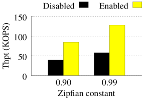
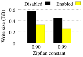
(a) Throughput	(b) Total write size

Figure 11: Experiment 6: Hotness awareness.

Experiment 7 (Selective KV separation):

We evaluate the impact of selective KV separation on the update performance of HashKV. We consider three ratios of small-to-large KV pairs, including 1:2, 1:1, and 2:1. We set the small KV pair size as 40 B, and the large KV pair size as 1 KiB or 4 KiB. Recall that we set the threshold of selective KV separation as 192 B by default (§3.5), so when selective KV separation is enabled, the small KV pairs are stored entirely in the LSM-tree, while the large KV pairs are stored via KV separation. Figure 12 shows the results when selective KV separation is disabled or enabled. When selective KV separation is enabled, the throughput increases by 23.2-118.0% and 19.2-52.1% when the large KV pair size is 1 KiB and 4 KiB, respectively. We observe higher performance gain for workloads with a higher ratio of small KV pairs, due to the high update overhead of small KV pairs stored under KV separation. Also, selective KV separation reduces the total write size by 14.1-39.6% and 4.1-10.7% when the large KV pair size is 1 KiB and 4 KiB, respectively.

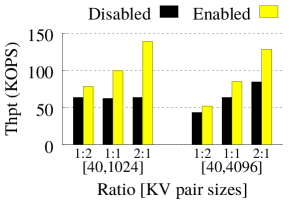
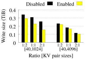
(a) Throughput	(b) Total write size

Figure 12: Experiment 7: Selective KV separation.

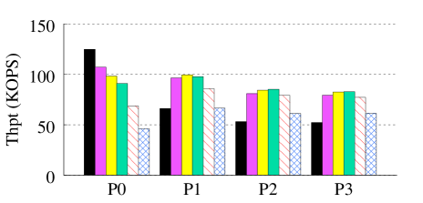
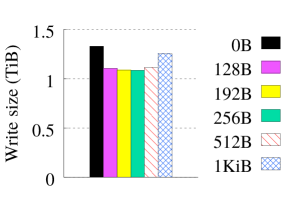
(a) Throughput	(b) Total write size

Figure 13: Experiment 8: Threshold selection of selective KV separation in HashKV under update-intensive workloads.

Experiment 8 (Threshold selection of selective KV separation):

We study the impact of the KV pair size threshold on the performance of selective KV separation. We consider different thresholds; when the threshold is 0 B, it implies that KV separation is always used. We modify the update-intensive workloads in §4.2 by generating KV pairs of different sizes ranging from 40 B to 8 KiB based on a Zipf distribution with a Zipfian constant of 0.99 (note that we have also evaluated the case where the KV pairs have sizes ranging from 40 B to 16 KiB and observed similar results). To ensure that different KV pair sizes are sufficiently covered, we increase the volume of KV pairs being inserted or updated to 120 GiB in each phase (i.e., 3$\times$ of the data volume in the original update-intensive workloads in §4.2), and configure 120 GiB of storage space with 30% of reserved space.

Figures 13(a) shows the throughput of HashKV under the update-intensive workloads. In the load phase (Phase P0), the throughput decreases when the threshold increases, since HashKV loads more KV pairs into LevelDB and triggers more compaction operations. In the update phases (Phases P1-P3), the throughput of HashKV first increases and then decreases with the increasing threshold. Note that HashKV reaches the maximum update throughput when the threshold is in the range from 128 B to 256 B, in which the update throughput is at least 40% higher compared to the threshold 0 B (i.e., KV separation is always used). Also, the throughput is similar for the thresholds of 128 B, 192 B, and 256 B. We further evaluate the impact of the threshold selection via YCSB benchmarking in §4.5.

Figure 13(b) shows the total write size of HashKV under the update-intensive workloads. When the threshold is in the range from 128 B to 512 B, HashKV reduces the write size by 16.9-18.4%.

Experiment 9 (Impact of GC approaches):

We study the impact of different GC approaches on the performance of HashKV (§3.3). We compare three variants of GC approaches with our default greedy approach: (i) CBA, (ii) GRA with $d=5$, and (iii) the random approach (i.e., GRA with $d$ set to the total number of segment groups). We evaluate the performance of HashKV under the update-intensive workloads, and consider two Zipfian constants, 0.9 and 0.99, as in Experiment 7.

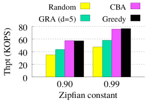
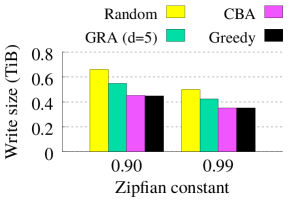
(a) Throughput	(b) Total write size

Figure 14: Experiment 9: Impact of GC approaches.

Figure 14(a) shows the update throughput of HashKV using different GC approaches under the update-intensive workloads. The update throughput of HashKV using the greedy approach is similar to that using CBA, and we find that the priority of choosing which segment group for GC is mainly determined by the amount of free space that can be reclaimed rather than the segment age. The update throughput of HashKV using the greedy approach is 61.3-62.2% and 31.5-32.1% higher than that using the Random and GRA approaches, respectively.

Figure 14(b) shows the total write size of HashKV using different GC approaches under the update-intensive workloads. Again, both the greedy and CBA approaches have similar write sizes. The greedy approach reduces the write size of using the random and GRA approaches by 30.1-32.0% and 17.5-18.4%, respectively.

Our results confirm that the default greedy approach in HashKV can achieve high update throughput and reduce the total write size.

Experiment 10 (Crash consistency):

We study the impact of the crash consistency mechanism on the performance of HashKV. Table 2 shows the results. When the crash consistency mechanism is enabled, the update throughput of HashKV in Phase P3 reduces by 6.5% and the total write size increases by 4.2%, which shows that the impact of crash consistency mechanism remains limited. Note that we verify the correctness of the crash consistency mechanism by crashing HashKV via code injection and unexpected terminations during runtime.

	Disabled	Enabled
Throughput (KOPS)	58.0	54.3
Total write size (GiB)	454.6	473.7

Table 2: Experiment 10: Performance of HashKV with crash consistency disabled and enabled.

4.5 Performance under YCSB Core Workloads

We study the performance of HashKV under the default YCSB core workloads [8] (Table 3). We do not consider Workload E, which is about range scans, and we will specifically study the effects of range scans for different KV pair sizes in Experiment 13 (see also Experiment 5). Here, we focus on the aged KV stores that have executed a large number of updates. Specifically, before running each YCSB workload, we first run Phases P0-P2 on each KV store; in this case, both vLog and HashKV have started to trigger GC in their value stores. We then run each YCSB workload based on the storage layout after issuing the update-intensive workloads, and fix the KV pair size as 1 KiB by default. In addition, we set the MemTable size, level0-slowdown, and level0-stop of RocksDB to 4 MiB, 8, and 12, respectively, so as to match the default parameters of LevelDB, HyperLevelDB, and PebblesDB.

Experiment 11 (YCSB benchmarking):

We first present the performance results of LevelDB, RocksDB, HyperLevelDB, PebblesDB, vLog, and HashKV under the default YCSB core workloads. Figures 15(a) and 15(b) show the aggregate throughput and the 95th percentile read latency of each KV store, respectively, under each YCSB workload.

We start with considering Workload A and Workload F, both of which contain around 50% of reads. The throughput of HashKV is 2.8-2.9$\times$, 3.2-3.6$\times$, 1.8-2.0$\times$, and 1.1-1.4$\times$ over LevelDB, HyperLevelDB, PebblesDB, and vLog, respectively. We observe that LevelDB, HyperLevelDB, and PebblesDB also have higher read latencies, which also lead to less overall throughput. Both vLog and HashKV have similar read latencies, yet vLog has lower throughput than HashKV due to the GC overhead. However, the throughput of HashKV is 12.5-13.9% lower than RocksDB, mainly because RocksDB no longer stalls writes for flushing the MemTable under the workloads with less intensive updates and it can better serve reads and updates via multi-threading optimization [15]. Nevertheless, we show that HashKV can achieve higher throughput when it uses RocksDB, instead of LevelDB, for key and metadata management (Experiment 13).

We next consider Workload B, Workload C, and Workload D, all of which are read-intensive. HashKV, vLog, and RocksDB have similar read latencies and hence similar throughput. HashKV achieves 2.3-4.8$\times$, 3.2-4.4$\times$, and 2.3-3.1$\times$ throughput over LevelDB, HyperLevelDB, and PebblesDB, respectively.

Workload	Portions of Requests
A (Update-heavy)	50% updates, 50% reads
B (Read-mostly)	5% updates, 95% reads
C (Read-only)	100% reads
D (Read-latest)	5% inserts, 95% reads
F (Read-modify-write)	50% read-modify-write, 50% reads

Table 3: YCSB core workloads [8].

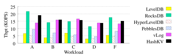
(a) Aggregate throughput

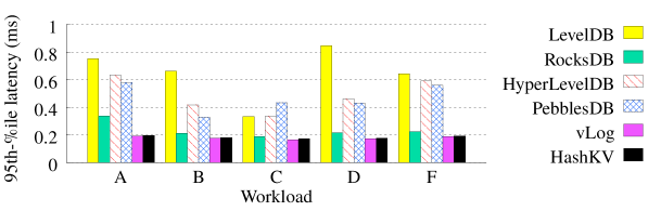
(b) 95th percentile read latency

Figure 15: Experiment 11: YCSB benchmarking.

Experiment 12 (Threshold selection of selective KV separation):

We study the impact of the KV pair size threshold on the performance of HashKV under YCSB core workloads. We use the same experiment setting as in Experiment 8 (i.e., we vary the KV pair size from 40 B to 8 KiB following the Zipf distribution with a Zipfian constant of 0.99 and configure 120 GiB of storage space with 30% of reserved space). Figure 16(a) shows the aggregate throughput of HashKV for different KV pair size thresholds. For all workloads, HashKV achieves the maximum throughput when the threshold is in the range of 128 B and 256 B, and improves the throughput by 26.5-48.3% compared to the threshold 0 B (i.e., KV separation is always used). Figure 16(b) shows the 95th percentile read latency of HashKV under the YCSB core workloads. Again, the read latency is the lowest when the threshold is in the range of 128 B and 256 B. From Experiment 8 and this experiment, we see that our threshold selection approach in §3.5 remains robust across different workloads.

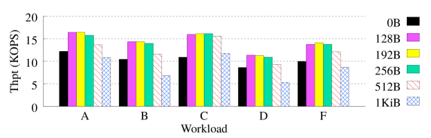
(a) Aggregate throughput

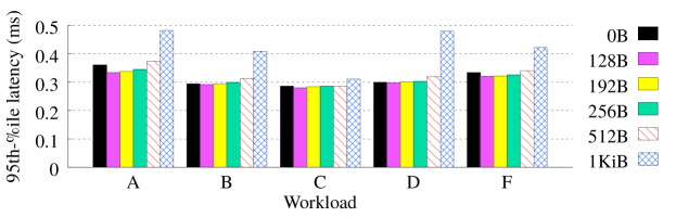
(b) 95th percentile read latency

Figure 16: Experiment 12: Threshold selection of selective KV separation under YCSB core workloads.

Experiment 13 (Deployment of KV separation on different KV stores):

We study the performance of two KV separation designs, HashKV and vLog, when we deploy KV separation on different KV stores. Specifically, we configure HashKV and vLog to use RocksDB, HyperLevelDB, and PebblesDB, instead of LevelDB, as the LSM-tree implementation for key and metadata management. For clarity, we append the suffixes “-RDB”, “-HDB”, and “-PDB” to HashKV and vLog to denote their deployment on RocksDB, HyperLevelDB, and PebblesDB, respectively.

Figure 17 shows the deployment of HashKV and vLog on RocksDB, HyperLevelDB, and PebblesDB, under YCSB core workloads. We first compare the performance of HashKV and vLog to the KV stores without KV separation. Both HashKV and vLog increase the aggregate throughput of each KV store across different YCSB core workloads via KV separation. For example, under Workload A and Workload F (i.e., the update-intensive workloads), the throughput of HashKV-RDB, HashKV-HDB, and HashKV-PDB is 1.2$\times$, 4.6-5.0$\times$, and 2.2-2.4$\times$ over RocksDB, HyperLevelDB, and PebblesDB, respectively. Also, HashKV still outperforms vLog: the throughput of HashKV-RDB, HashKV-HDB, and HashKV-PDB is 21.3-39.4%, 10.7-22.5%, and 48.5-91.0% higher than vLog-RDB, vLog-HDB, and vLog-PDB, respectively. Under Workload B, Workload C, and Workload D (i.e., the read-intensive workloads), the throughput of HashKV-RDB, HashKV-HDB, and HashKV-PDB is 1.1-1.3$\times$, 3.9-5.6$\times$, and 2.0-2.6$\times$ over RocksDB, HyperLevelDB, and PebblesDB, respectively. Both HashKV and vLog achieve similar throughput under the read-intensive workloads when they are deployed over the same KV store.

We further compare the range scan performance of HashKV and vLog to the KV stores without KV separation. We consider the same range scan workload as in Experiment 5 (§4.3). Figure 18 shows the range scan performance of HashKV and vLog when they are deployed on RocksDB, HyperLevelDB, and PebblesDB. Overall, HashKV has similar range scan performance to vLog for most KV pair sizes in all cases. Also, both of them achieve similar or higher range scan performance than RocksDB for larger KV pair sizes due to KV separation.

Note that the range scan throughput of PebblesDB is significantly lower than that of RocksDB and HyperLevelDB. The reason is that PebblesDB triggers a number of compaction operations during range scans, and such compaction overhead significantly degrades the range scan performance especially for large KV pairs. Also, PebblesDB’s fragmented LSM-tree design causes the KV pairs to be scattered across multiple levels, and each range scan needs to examine multiple levels to retrieve all KV pairs (see [38] for details). Nevertheless, KV separation (under HashKV or vLog) significantly improves the range scan performance.

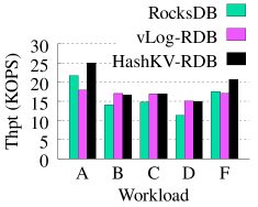
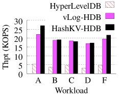
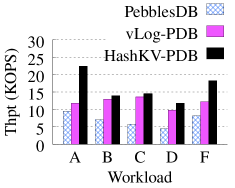
(a) RocksDB	(b) HyperLevelDB	(c) PebblesDB

Figure 17: Experiment 13: Deployment of KV separation on different KV stores under YCSB core workloads.

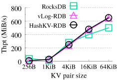
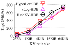
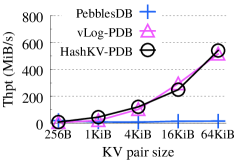
(a) RocksDB	(b) HyperLevelDB	(c) PebblesDB

Figure 18: Experiment 13: Impact of KV separation on different KV stores under range scan workloads.

(a) Cumulative distribution of KV pairs among segment groups after Phase P0	(b) Storage space utilization after each of Phases P1-P3

Figure 19: Experiment 14: Storage distribution of KV pairs in HashKV.

4.6 Storage Distribution of KV Pairs

Experiment 14 (Storage distribution of KV pairs)

: We study the storage distribution of KV pairs in HashKV under the update-intensive workloads in §4.2. Since HashKV distributes KV pairs via hashing, it is possible that the KV pairs are unevenly distributed across segment groups and some segment groups are not fully utilized. However, if there are a sufficiently large number of keys and the hash function can produce uniformly distributed outputs, we argue that the KV pairs are indeed evenly distributed across segment groups. Figure 19(a) plots the cumulative distribution of the number of KV pairs across segment groups at the end of the load phase (Phase P0). We see that the number of KV pairs in each segment group varies between 64K and 66K, and the difference is within 2.5% only.

Also, we argue that update-intensive workloads have limited impact on storage space utilization (i.e., the fraction of valid and invalid data being stored over the entire storage space), even though some segment groups may allocate new log segments after receiving extensive updates (§3.2). Figure 19(b) shows the utilization of the storage space at the end of each update phase (i.e., Phases P1-P3). HashKV achieves a high utilization of 99.4% across the update phases.

4.7 Parameter Choices

We further study the impact of parameters, including the main segment size, the log segment size, and the write cache size on the update performance of HashKV under the update-intensive workloads in §4.2. We vary one parameter in each test, and use the default values for other parameters. We report the update throughput in Phase P3 and the total write size. Here, we focus on 20% and 50% of reserved space.

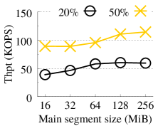
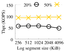
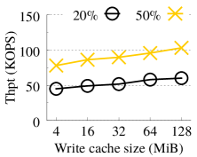
(a)	(b)	(c)
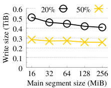
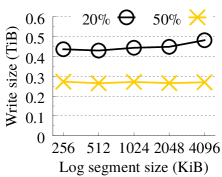
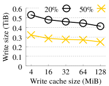
(d)	(e)	(f)

Figure 20: Experiment 15: Throughput and total write size of HashKV versus the main segment size ((a) and (d)), the log segment size ((b) and (e)), and the write cache size ((c) and (f)).

Experiment 15 (Impact of main segment size, log segment size, and write cache size):

We first consider the main segment size. Figures 20(a) and 20(d) show the results versus the main segment size. When the main segment size increases, the throughput of HashKV increases, while the total write size decreases. The reason is that there are fewer segment groups for larger main segments, so each segment group receives more updates in general. Each GC operation can now reclaim more space from more updates, so the performance improves. We see that the update performance of HashKV is more sensitive to the main segment size under limited reserved space. For example, the throughput increases by 52.5% under 20% of reserved space, but 28.3% under 50% of reserved space, when the main segment size increases from 16 MiB to 256 MiB.

We next consider the log segment size. Figures 20(b) and 20(e) show the results versus the log segment size. We see that when the log segment size increases from 256 KiB to 4 MiB, the throughput of HashKV drops by 16.1%, while the write size increases by 10.4% under 20% of reserved space. The reason is that the utilization of log segments decreases as the log segment size increases. Thus, each GC operation reclaims less free space, and the performance drops. However, when the reserved space size increases to 50%, we do not see significant performance differences, and both the throughput and the write size remain almost unchanged across different log segment sizes.

We finally consider the write cache size. Figures 20(c) and 20(f) show the results versus the write cache size. As expected, the throughput of HashKV increases and the total write size drops as the write cache size increases, since a larger write cache can absorb more updates. For example, under 20% of reserved space, the throughput of HashKV increases by 29.1% and the total write size reduces by 16.3% when the write cache size increases from 4 MiB to 64 MiB.

5 Related Work

General KV stores: Many KV store designs are proposed for different types of storage backends, such as DRAM [17, 39, 16, 26], commodity flash-based SSDs [9, 10, 25, 28], open-channel SSDs [43], and emerging non-volatile memories [31, 50]. The above KV stores and HashKV are designed for a single server. They can serve as building blocks of a distributed KV store (e.g., [34]).

LSM-tree-based KV stores:

As stated in §1, the LSM-tree [35] is a major building block for most today’s KV stores that target workloads with high volumes of inserts or updates. Many studies extend the LSM-tree design for improved compaction performance; we refer readers to the survey [29] on state-of-the-art LSM-tree-based KV stores. To name a few, bLSM [42] proposes a new merge scheduler to prevent the compaction operations from blocking write requests, and uses Bloom filters for efficient indexing. VT-Tree [44] stitches already sorted blocks of SSTables to allow lightweight compaction overhead, at the expense of incurring fragmentation. LSM-trie [49] maintains a trie structure and organizes KV pairs by hash-based buckets within each SSTable. It also organizes large Bloom filters in clustered disk blocks for efficient I/O access. LWC-store [51] decouples data and metadata management in compaction by merging and sorting only the metadata in SSTables. SkipStore [52] pushes KV pairs across non-adjacent levels to reduce the number of levels traversed during compaction. TRIAD [3] combines different techniques to reduce compaction overhead, and addresses data skewness by keeping hot data in memory while flushing only cold data into disk (note that our write cache also buffers recently written KV pairs and allows them to be directly updated in-place). PebblesDB [38] relaxes the restriction of keeping disjoint key ranges in each level, and pushes partial SSTables across levels to limit compaction overhead. LSbM [45] keeps frequently accessed KV pairs in a compaction buffer to avoid cache invalidation caused by compaction, thereby improving read performance. Note that the aforementioned LSM-tree-based KV stores do not address KV separation. Their performance is still limited by the compaction and lookup overheads due to the storage of values in the LSM-tree (see Experiment 13 in §4.5).

KV separation:

WiscKey [28] employs KV separation to remove value compaction in the LSM-tree (see §2.2). Atlas [22] also applies KV separation in cloud storage, in which keys and metadata are stored in an LSM-tree that is replicated, while values are separately stored and erasure-coded for low-redundancy fault tolerance. Cocytus [53] is an in-memory KV store that separates keys and values for replication and erasure coding, respectively. Tucana [37] uses a B^ϵ-tree for indexing, so as to reduce the I/O amplifications compared to the LSM-tree. Similar to WiscKey, Tucana employs KV separation and stores the values in an append-only log. While HashKV also builds on KV separation, it takes one step further to address efficient GC management in value storage via hash-based data grouping.

GC in log-structured storage:

Many efficient GC designs have been proposed for log-structured storage, including log-structured file systems [40, 32, 41] and SSDs [33, 23], yet applying them directly to LSM-tree-based KV storage is challenging (§2.2). For KV storage, Berkeley DB [36] maintains no-overwrite log files, and selects the log file with the fewest active records for GC. BadgerDB [12], a WiscKey-based implementation in Golang, divides the value store into regions. It leverages the statistics obtained from LSM-tree compaction to identify the regions with the most free space for GC. In contrast, HashKV specifically aims for efficient GC in LSM-tree-based KV separation via hash-based data grouping, which eliminates the need of querying the LSM-tree during GC. We also show how hash-based data grouping can be extended with hotness awareness.

Hash-based data organization:

Distributed storage systems (e.g., [48, 11, 30]) use hash-based data placement to avoid centralized metadata lookups. NVMKV [31] also uses hashing to map KV pairs in physical address space. However, it assumes sparse address space to limit the overhead of resolving hash collisions, and incurs internal fragmentation for small-sized KV pairs. In contrast, HashKV does not cause internal fragmentation as it packs KV pairs in each main/log segment in a log-structured manner. It also supports dynamic reserved space allocation when the main segments become full.

6 Conclusion

This paper presents HashKV, which enables efficient updates in KV stores under update-intensive workloads. Its novelty lies in leveraging hash-based data grouping for deterministic data organization so as to mitigate GC overhead. We also enhance HashKV with several extensions including dynamic reserved space allocation, hotness awareness, and selective KV separation. Testbed experiments show that HashKV achieves high update throughput and reduces the total write size. We further demonstrate that HashKV can build on different LSM-tree-based KV stores to improve their respective performance.

References

- [1] N. Agrawal, V. Prabhakaran, T. Wobber, J. D. Davis, M. Manasse, and R. Panigrahy. Design Tradeoffs for SSD Performance. In Proceedings of the 2008 USENIX Annual Technical Conference (ATC’08), pages 57–70, 2008.
- [2] B. Atikoglu, Y. Xu, E. Frachtenberg, S. Jiang, and M. Paleczny. Workload Analysis of a Large-Scale Key-Value Store. In Proceedings of the 12th ACM SIGMETRICS/PERFORMANCE Joint International Conference on Measurement and Modeling of Computer Systems (SIGMETRICS’12), pages 53–64, 2012.
- [3] O. Balmau, D. Didona, R. Guerraoui, W. Zwaenepoel, H. Yuan, A. Arora, K. Gupta, and P. Konka. TRIAD: Creating Synergies Between Memory, Disk and Log in Log Structured Key-Value Stores. In Proceedings of the 2017 USENIX Annual Technical Conference (ATC’17), pages 363–375, 2017.
- [4] D. Beaver, S. Kumar, H. C. Li, J. Sobel, and P. Vajgel. Finding a Needle in Haystack: Facebook’s Photo Storage. In Proceedings of the 9th USENIX Symposium on Operating Systems Design and Implementation (OSDI’10), pages 47–60, 2010.
- [5] H. H. W. Chan, Y. Li, P. P. C. Lee, and Y. Xu. HashKV: Enabling Efficient Updates in KV Storage via Hashing. In Proceedings of the 2018 USENIX Annual Technical Conference (ATC’18), pages 1007–1019, 2018.
- [6] F. Chang, J. Dean, S. Ghemawat, W. C. Hsieh, D. A. Wallach, M. Burrows, T. Chandra, A. Fikes, and R. E. Gruber. Bigtable: A Distributed Storage System for Structured Data. In Proceedings of the 7th USENIX Symposium on Operating Systems Design and Implementation (OSDI’06), pages 15–15, 2006.
- [7] Y. L. Chen, S. Mu, J. Li, C. Huang, J. Li, A. Ogus, and D. Phillips. Giza: Erasure Coding Objects across Global Data Centers. In Proceedings of the 2017 USENIX Annual Technical Conference (ATC’17), pages 539–551, 2017.
- [8] B. F. Cooper, A. Silberstein, E. Tam, R. Ramakrishnan, and R. Sears. Benchmarking Cloud Serving Systems with YCSB. In Proceedings of the 1st ACM Symposium on Cloud Computing (SoCC’10), pages 143–154, 2010.
- [9] B. Debnath, S. Sengupta, and J. Li. FlashStore: High Throughput Persistent Key-value Store. Proceedings of the VLDB Endowment, 3(1-2):1414–1425, Sep 2010.
- [10] B. Debnath, S. Sengupta, and J. Li. SkimpyStash: RAM Space Skimpy Key-value Store on Flash-based Storage. In Proceedings of the 2011 ACM SIGMOD International Conference on Management of Data (SIGMOD’11), pages 25–36, 2011.
- [11] G. DeCandia, D. Hastorun, M. Jampani, G. Kakulapati, A. Lakshman, A. Pilchin, S. Sivasubramanian, P. Vosshall, and W. Vogels. Dynamo: Amazon’s Highly Available Key-value Store. In Proceedings of the 21st ACM SIGOPS Symposium on Operating Systems Principles (SOSP’07), pages 205–220, 2007.
- [12] Dgraph Labs. BadgerDB. https://github.com/dgraph-io/badger/, Retrieved June 2019.
- [13] R. Escriva. HyperLevelDB. https://github.com/rescrv/HyperLevelDB/, Retrieved in June 2019.
- [14] Facebook. RocksDB. https://rocksdb.org, Retrieved in June 2019.
- [15] Facebook. RocksDB Features that are not in LevelDB. https://github.com/facebook/rocksdb/wiki/Features-Not-in-LevelDB, Retrieved in June 2019.
- [16] B. Fan, D. G. Andersen, and M. Kaminsky. MemC3: Compact and Concurrent MemCache with Dumber Caching and Smarter Hashing. In Proceedings of the 10th USENIX Conference on Networked Systems Design and Implementation (NSDI’13), pages 371–384, 2013.
- [17] B. Fitzpatrick. Distributed Caching with Memcached. Linux Journal, 2004(124), Aug 2004.
- [18] S. Ghemawat and J. Dean. LevelDB. https://leveldb.org, Retrieved in June 2019.
- [19] N. Griffiths. nmon for Linux. http://nmon.sourceforge.net/, Retrieved in June 2019.
- [20] J.-W. Hsieh, T.-W. Kuo, and L.-P. Chang. Efficient Identification of Hot Data for Flash Memory Storage Systems. ACM Transactions on Storage, 2(1):22–40, Feb 2006.
- [21] S. Kavalanekar, B. Worthington, Q. Zhang, and V. Sharda. Characterization of Storage Workload Traces from Production Windows Servers. In Proceedings of the 2008 IEEE International Symposium on Workload Characterization (IISWC’08), pages 119–128, 2008.
- [22] C. Lai, S. Jiang, L. Yang, S. Lin, G. Sun, Z. Hou, C. Cui, and J. Cong. Atlas: Baidu’s Key-value Storage System for Cloud Data. In Proceedings of the 31st Symposium on Mass Storage Systems and Technologies (MSST’15), pages 1–14, 2015.
- [23] J. Lee and J.-S. Kim. An Empirical Study of Hot/Cold Data Separation Policies in Solid State Drives (SSDs). In Proceedings of the 6th International Systems and Storage Conference (SYSTOR’13), page 12, 2013.
- [24] Y. Li, P. P. Lee, J. C. Lui, and Y. Xu. Impact of Data Locality on Garbage Collection in SSDs: A General Analytical Study. In Proceedings of the 6th ACM/SPEC International Conference on Performance Engineering (ICPE’15), pages 305–315, 2015.
- [25] H. Lim, B. Fan, D. G. Andersen, and M. Kaminsky. SILT: A Memory-Efficient, High-Performance Key-Value Store. In Proceedings of the 23rd ACM Symposium on Operating Systems Principles (SOSP’11), pages 1–13, 2011.
- [26] H. Lim, D. Han, D. G. Andersen, and M. Kaminsky. MICA: A Holistic Approach to Fast In-Memory Key-Value Storage. In Proceedings of the 11th USENIX Conference on Networked Systems Design and Implementation (NSDI’14), pages 429–444, 2014.
- [27] Linux Raid Wiki. RAID setup. https://raid.wiki.kernel.org/index.php/RAID_setup, Retrieved in June 2019.
- [28] L. Lu, T. S. Pillai, A. C. Arpaci-Dusseau, and R. H. Arpaci-Dusseau. WiscKey: Separating Keys from Values in SSD-Conscious Storage. ACM Transactions on Storage, 13(1):5, Mar 2017.
- [29] C. Luo and M. J. Carey. LSM-based Storage Techniques: A Survey. CoRR, abs/1812.07527, Dec 2018. http://arxiv.org/abs/1812.07527.
- [30] J. MacCormick, N. Murphy, V. Ramasubramanian, U. Wieder, J. Yang, and L. Zhou. Kinesis: A New Approach to Replica Placement in Distributed Storage Systems. ACM Transactions on Storage, 4(4):11, 2009.
- [31] L. Marmol, S. Sundararaman, N. Talagala, and R. Rangaswami. NVMKV: A Scalable, Lightweight, FTL-aware Key-Value Store. In Proceedings of the 2015 USENIX Annual Technical Conference (ATC’15), pages 207–219, 2015.
- [32] J. N. Matthews, D. Roselli, A. M. Costello, R. Y. Wang, and T. E. Anderson. Improving the Performance of Log-Structured File Systems with Adaptive Methods. In Proceedings of the 16th ACM Symposium on Operating Systems Principles (SOSP’97), pages 238–251, 1997.
- [33] C. Min, K. Kim, H. Cho, S.-W. Lee, and Y. I. Eom. SFS: Random Write Considered Harmful in Solid State Drives. In Proceedings of the 10th USENIX Conference on File and Storage Technologies (FAST’12), pages 12–12, 2012.
- [34] R. Nishtala, H. Fugal, S. Grimm, M. Kwiatkowski, H. Lee, H. C. Li, R. McElroy, M. Paleczny, D. Peek, P. Saab, D. Stafford, T. Tung, and enkateshwaran Venkataramani. Scaling Memcache at Facebook. In Proceedings of the 10th USENIX Conference on Networked Systems Design and Implementation, pages 385–398, 2013.
- [35] P. O’Neil, E. Cheng, D. Gawlick, and E. O’Neil. The Log-Structured Merge-Tree (LSM-tree). Acta Informatica, 33(4):351–385, 1996.
- [36] Oracle. Oracle Berkeley DB, Java Edition - Getting Started with Berkeley DB Java Edition - 12c Release 2 Library Version 12.2.7.5, Oct 2017.
- [37] A. Papagiannis, G. Saloustros, P. González-Férez, and A. Bilas. Tucana: Design and Implementation of a Fast and Efficient Scale-up Key-value Store. In Proceedings of the 2016 USENIX Annual Technical Conference (ATC’16), pages 537–550, 2016.
- [38] P. Raju, R. Kadekodi, V. Chidambaram, and I. Abraham. PebblesDB: Building Key-Value Stores using Fragmented Log-Structured Merge Trees. In Proceedings of the 26th Symposium on Operating Systems Principles (SOSP’17), pages 497–514, 2017.
- [39] Redis. http://redis.io, Retrieved in June 2019.
- [40] M. Rosenblum and J. K. Ousterhout. The Design and Implementation of a Log-structured File System. ACM Transactions on Computer Systems, 10(1):26–52, Feb 1992.
- [41] S. M. Rumble, A. Kejriwal, and J. Ousterhout. Log-structured Memory for DRAM-based Storage. In Proceedings of the 12th USENIX conference on File and Storage Technologies (FAST’16), pages 1–16, 2014.
- [42] R. Sears and R. Ramakrishnan. bLSM: A General Purpose Log Structured Merge Tree. In Proceedings of the 2012 ACM SIGMOD International Conference on Management of Data (SIGMOD’12), pages 217–228, 2012.
- [43] Z. Shen, F. Chen, Y. Jia, and Z. Shao. DIDACache: A Deep Integration of Device and Application for Flash Based Key-Value Caching. ACM Transactions on Storage, 14(3):26, Nov 2018.
- [44] P. J. Shetty, R. P. Spillane, R. R. Malpani, B. Andrews, J. Seyster, and E. Zadok. Building Workload-Independent Storage with VT-Trees. In Proceedings of the 11th USENIX Conference on File and Storage Technologies (FAST’13), pages 17–30, 2013.
- [45] D. Teng, L. Guo, R. Lee, F. Chen, Y. Zhang, S. Ma, and X. Zhang. A Low-cost Disk Solution Enabling LSM-tree to Achieve High Performance for Mixed Read/Write Workloads. ACM Transactions on Storage, 14(2):15:1–15:26, 2018.
- [46] Threadpool. http://threadpool.sourceforge.net/, Retrieved in June 2019.
- [47] TPC. TPC-C is an On-Line Transaction Processing Benchmark. http://www.tpc.org/tpcc/, Retrieved in June 2019.
- [48] S. A. Weil, S. A. Brandt, E. L. Miller, D. D. E. Long, and C. Maltzahn. Ceph: A Scalable, High-Performance Distributed File System. In Proceedings of the 7th USENIX Symposium on Operating Systems Design and Implementation (OSDI’06), pages 307–320, 2006.
- [49] X. Wu, Y. Xu, Z. Shao, and S. Jiang. LSM-trie: An LSM-tree-based Ultra-Large Key-Value Store for Small Data. In Proceedings of the 2015 USENIX Annual Technical Conference (ATC’15), pages 71–82, 2015.
- [50] F. Xia, D. Jiang, J. Xiong, and N. Sun. HiKV: A Hybrid Index Key-Value Store for DRAM-NVM Memory Systems. In Proceedings of the 2017 USENIX Annual Technical Conference (ATC’17), pages 349–362, 2017.
- [51] T. Yao, J. Wan, P. Huang, X. He, Q. Gui, F. Wu, and C. Xie. A Light-weight Compaction Tree to Reduce I/O Amplification toward Efficient Key-Value Stores. In Proceedings of the 33rd International Conference on Massive Storage Systems and Technology (MSST’17), 2017.
- [52] Y. Yue, B. He, Y. Li, and W. Wang. Building an Efficient Put-Intensive Key-Value Store with Skip-Tree. IEEE Transactions on Parallel and Distributed Systems, 28(4):961–973, Apr 2017.
- [53] H. Zhang, M. Dong, and H. Chen. Efficient and Available In-memory KV-Store with Hybrid Erasure Coding and Replication. ACM Transactions on Storage, 13(3):25, Oct 2017.