Spectral form factor and semi-circle law in the time direction

Abstract

We study the time derivative of the connected part of spectral form factor, which we call the slope of ramp, in Gaussian matrix model. We find a closed formula of the slope of ramp at finite $N$ with non-zero inverse temperature. Using this exact result, we confirm numerically that the slope of ramp exhibits a semi-circle law as a function of time.

1 Introduction

After the seminal work Garcia-Garcia:2016mno ; Cotler:2016fpe , the spectral form factor is intensively studied as a diagnostic of the quantum chaotic behavior of the Sachdev-Ye-Kitaev (SYK) model KitaevTalks ; Sachdev ; Maldacena:2016hyu , which is a solvable example of the holographic model of a certain black hole in two-dimension. At late times, the spectral form factor of SYK model exhibits a structure of the so-called ramp and plateau, and it is well-approximated by the behavior of the Gaussian Unitary Ensemble (GUE) random matrix model when the number of fermions mod 8 is 2 or 6 you .

In this paper, we will consider the the spectral form factor $g(\beta,t)$ in GUE matrix model with non-zero inverse temperature $\beta$. We will show that $g(\beta,t)$ is written exactly as a trace of an $N\times N$ matrix $A(z)$ defined in (8). $g(\beta,t)$ consists of two parts: the disconnected part $g_{\text{disc}}(\beta,t)$ (12) and the connected part $g_{\text{conn}}(\beta,t)$ (13). In Figure 1, we show the plot of this exact $g(\beta,t)$ for $\beta=5$ with the matrix size $N=500$. As we can see from Figure 1, after the initial decay described by the disconnected part $g_{\text{disc}}(\beta,t)$, $g(\beta,t)$ has the structure of ramp and plateau at late times. This late time behavior comes from the connected part $g_{\text{conn}}(\beta,t)$ and it was studied extensively in the literature (see e.g. hikami ; Liu:2018hlr and references therein).

The ramp is closely related to the short range correlation of eigenvalues described by the so-called sine kernel, and if we focus on the contribution from a small window around some fixed eigenvalue the ramp grows linearly in $t$. However, since $g(\beta,t)$ is defined by integrating over the whole range of eigenvalue distribution, the actual ramp is not a linear function of $t$.

In this paper, we will study the non-linearity of ramp using the exact result at finite $N$. To see the deviation from the linear behavior, it is natural to consider the time derivative of $g_{\text{conn}}(\beta,t)$, which we will call the slope of ramp. If the ramp were a linear function of $t$, the slope of ramp would be a constant. However, the actual slope of ramp is not constant in time. It turns out that the slope of ramp obeys the semi-circle law as a function of time. This is a direct consequence of the semi-circle law of eigenvalue distribution, of course, but there is an interesting twist: the slope of ramp corresponds to the eigenvalues and the time corresponds to the eigenvalue density (see Figure 2 for the detail of this correspondence). In other words, the eigenvalue density manifests itself as the time direction in the graph of the slope of ramp.

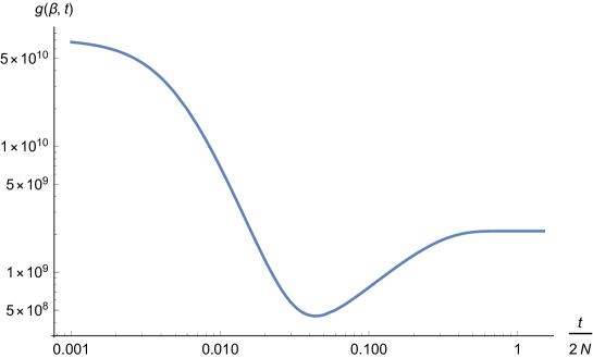
Figure 1: Plot of the exact spectral form factor $g(\beta,t)$ in GUE for $\beta=5,N=500$.

This paper is organized as follows. In section 2, we write down the exact closed form expression of the slope of ramp $\partial_{t}g_{\text{conn}}(\beta,t)$ at finite $N$. In section 3, we compute the late time behavior of $g_{\text{conn}}(\beta,t)$ in the large $N$ limit. We point out that after an appropriate change of variable (34), the slope of ramp obeys the semi-circle law as a function of time. In section 4, we plot the slope of ramp as a function of time using our exact result at finite $N$ for both $\beta=0$ and $\beta\neq 0$ cases, and confirm that the slope of ramp exhibits the semi-circle law. In section 5, we consider the slope of ramp in the small $t$ regime. Finally, we conclude in section 6. In Appendix A, we explain how to compute $\operatorname{Tr}A(z)$ and $\operatorname{Tr}A(z_{1})A(z_{2})$.

2 Exact slope of ramp at finite $N$

In this paper we consider the spectral form factor in Gaussian matrix model defined by

$$g(\beta,t)=\Bigl{\langle}\operatorname{Tr}e^{-(\beta+\mathrm{i}t)H}\operatorname{Tr}e^{-(\beta-\mathrm{i}t)H}\Bigr{\rangle} =\frac{\int dHe^{-\frac{N}{2}\operatorname{Tr}H^{2}}\operatorname{Tr}e^{-(\beta+\mathrm{i}t)H}\operatorname{Tr}e^{-(\beta-\mathrm{i}t)H}}{\int dHe^{-\frac{N}{2}\operatorname{Tr}H^{2}}},$$ (1)

where the integral is over the $N\times N$ hermitian matrix $H$. By definition, $g(\beta,t)$ is an even function of $t$. Moreover, since the Gaussian measure is invariant under $H\to-H$, $g(\beta,t)$ is independent of the sign of $\beta$. In the following we will assume that $\beta$ and $t$ are both positive without loss of generality:

$$\beta\geq 0,\quad t\geq 0.$$ (2)

In the normalization of Gaussian measure in (1), the eigenvalue $\mu$ of matrix $H$ is distributed along the cut $\mu\in[-2,2]$ in the large $N$ limit, and the eigenvalue density $\rho(\mu)$ is given by the Wigner semi-circle law

$$\rho(\mu)=\frac{1}{2\pi}\sqrt{4-\mu^{2}}.$$ (3)

As pointed out in delCampo:2017bzr , $g(\beta,t)$ in (1) is formally equivalent to the correlator of 1/2 BPS Wilson loops in 4d $\mathcal{N}=4$ Super Yang-Mills (SYM) theory, which is also given by the Gaussian matrix model via the supersymmetric localization Erickson:2000af ; Drukker:2000rr ; Pestun:2007rz . Thus, we can immediately find the exact form of $g(\beta,t)$ by borrowing the known result of $\mathcal{N}=4$ SYM in Drukker:2000rr ; Kawamoto:2008gp ; Okuyama:2018aij . To do this, it is convenient to rescale the matrix

$$H=\sqrt{\frac{2}{N}}M,$$ (4)

so that the measure becomes $\int dMe^{-\operatorname{Tr}M^{2}}$. In this normalization, $g(\beta,t)$ is written as

$$g(\beta,t)=\Bigl{\langle}\operatorname{Tr}e^{\frac{\beta+\mathrm{i}t}{\sqrt{N}}\sqrt{2}M}\operatorname{Tr}e^{\frac{\beta-\mathrm{i}t}{\sqrt{N}}\sqrt{2}M}\Bigr{\rangle}.$$ (5)

On the other hand, the correlator of 1/2 BPS Wilson loops with winding number $k_{i}$ is given by Okuyama:2018aij

$$\left\langle\prod_{i}\operatorname{Tr}e^{k_{i}\sqrt{\frac{\lambda}{4N}}\sqrt{2}M}\right\rangle,$$ (6)

where $\lambda$ denotes the ’t Hooft coupling of $\mathcal{N}=4$ SYM. Comparing (5) and (6), we find a dictionary between Wilson loops in $\mathcal{N}=4$ SYM and the spectral form factor

$$k_{i}\sqrt{\lambda}~{}\leftrightarrow~{}2(\beta\pm\mathrm{i}t).$$ (7)

As shown in Fiol:2013hna ; Okuyama:2018aij , the correlator of $\operatorname{Tr}e^{z\sqrt{2}M}$ is written in terms of the $N\times N$ symmetric matrix $A(z)$ defined by

$$A(z)_{i,j}=\sqrt{\frac{i!}{j!}}e^{\frac{z^{2}}{2}}z^{j-i}L_{i}^{j-i}(-z^{2}),\quad(i,j=0,\cdots,N-1),$$ (8)

where $L_{n}^{\alpha}(x)$ denotes the associated Laguerre polynomial. The one-point function is given by the trace of $A(z)$ (see Appendix A for a derivation of this result)

$$\Bigl{\langle}\operatorname{Tr}e^{z\sqrt{2}M}\Bigr{\rangle}=\operatorname{Tr}A(z)=e^{\frac{z^{2}}{2}}L_{N-1}^{1}(-z^{2}).$$ (9)

The spectral form factor $g(\beta,t)$ in (5) is a two-point function of $\operatorname{Tr}e^{z\sqrt{2}M}$ and $\operatorname{Tr}e^{\overline{z}\sqrt{2}M}$ with

$$z=\frac{\beta+\mathrm{i}t}{\sqrt{N}},\quad\overline{z}=\frac{\beta-\mathrm{i}t}{\sqrt{N}}.$$ (10)

One can naturally decompose $g(\beta,t)$ into the disconnected part $g_{\text{disc}}(\beta,t)$ and the connected part $g_{\text{conn}}(\beta,t)$

$$g(\beta,t)=g_{\text{disc}}(\beta,t)+g_{\text{conn}}(\beta,t).$$ (11)

The disconnected part is given by a product of one-point functions

$$g_{\text{disc}}(\beta,t)=\operatorname{Tr}A(z)\operatorname{Tr}A(\overline{z})=e^{\frac{z^{2}+\overline{z}^{2}}{2}}L_{N-1}^{1}(-z^{2})L_{N-1}^{1}(-\overline{z}^{2}),$$ (12)

where $z$ and $\overline{z}$ are defined in (10). This part is responsible for the early time decay of $g(\beta,t)$, which we will not consider in this paper.

The late time behavior of $g(\beta,t)$, the so-called ramp and plateau, comes form the connected part. Using the result in Drukker:2000rr ; Kawamoto:2008gp ; Okuyama:2018aij , $g_{\text{conn}}(\beta,t)$ is written as

$$g_{\text{conn}}(\beta,t) =\operatorname{Tr}\Bigl{[}A(z+\overline{z})-A(z)A(\overline{z})\Bigr{]}.$$ (13)

Since $z+\overline{z}=\frac{2\beta}{\sqrt{N}}$, the first term of (13) is independent of time and it sets the value of plateau

$$g_{\text{plateau}}(\beta) =\operatorname{Tr}A(z+\overline{z})=e^{\frac{2\beta^{2}}{N}}L_{N-1}^{1}\Bigl{(}-\frac{4\beta^{2}}{N}\Bigr{)}.$$ (14)

Using the result of Wilson loop in $\mathcal{N}=4$ SYM Erickson:2000af , the large $N$ limit of $g_{\text{plateau}}(\beta)$ with fixed $\beta$ is given by

$$g_{\text{plateau}}(\beta)\approx N\frac{I_{1}(4\beta)}{2\beta},$$ (16)

where $I_{n}(x)$ denotes the modified Bessel function of the first kind.

The non-trivial time dependence comes from the second term of (13)

$$g_{\text{ramp}}(\beta,t) =-\operatorname{Tr}\Bigl{[}A(z)A(\overline{z})\Bigr{]}.$$ (17)

In what follows, we will consider the time derivative of $g_{\text{ramp}}(\beta,t)$, which we call the slope of ramp. Since $g_{\text{plateau}}(\beta)$ is independent of time, the slope of ramp is equal to the time derivative of the connected part of spectral form factor

$$\frac{\partial g_{\text{ramp}}}{\partial t}(\beta,t)=\frac{\partial g_{\text{conn}}}{\partial t}(\beta,t).$$ (18)

As explained in Appendix A, we can write down a closed form expression of the slope of ramp

$$\frac{\partial g_{\text{conn}}}{\partial t}(\beta,t) =\frac{N}{\beta}e^{\frac{z^{2}+\overline{z}^{2}}{2}}\text{Im}\Bigl{[}L_{N}(-z^{2})L_{N-1}(-\overline{z}^{2})\Bigr{]}.$$ (19)

By taking the limit $\beta\to 0$ of (19), the slope of ramp for $\beta=0$ becomes

$$\frac{\partial g_{\text{conn}}}{\partial t}(0,t)=2te^{-\frac{t^{2}}{N}}\Biggl{[}L_{N-1}\Bigl{(}\frac{t^{2}}{N}\Bigr{)}L_{N-1}^{1}\Bigl{(}\frac{t^{2}}{N}\Bigr{)}-L_{N}\Bigl{(}\frac{t^{2}}{N}\Bigr{)}L_{N-2}^{1}\Bigl{(}\frac{t^{2}}{N}\Bigr{)}\Biggr{]}.$$ (20)

We are interested in the large $N$ limit of the slope of ramp (19) and (20). When $\beta=0$, as pointed out in hikami , $\partial_{t}g_{\text{conn}}(0,t)$ in (20) happens to be equal to the eigenvalue density in the Wishart-Laguerre ensemble, which is known to obey the semi-circle law in the large $N$ limit. However, the large $N$ limit of $\partial_{t}g_{\text{conn}}(\beta,t)$ with non-zero $\beta$ is not well studied in the literature. In section 3, we will numerically study the large $N$ behavior of the exact result (19) and (20).

Before doing this numerical study, in the next section we will review the analytic derivation of the large $N$ behavior of ramp in hikami ; Liu:2018hlr .

3 Large $N$ limit of the slope of ramp

The large $N$ limit of $g_{\text{conn}}(\beta,t)$ is written in terms of the connected part of the two-level correlation function $\rho^{(2)}(\mu_{1},\mu_{2})$

$$g_{\text{conn}}(\beta,t) =\int d\mu_{1}d\mu_{2}\rho^{(2)}(\mu_{1},\mu_{2})e^{(\beta+\mathrm{i}t)\mu_{1}}e^{(\beta-\mathrm{i}t)\mu_{2}}$$ (21)

$$=\int d\mu_{1}d\mu_{2}\rho^{(2)}(\mu_{1},\mu_{2})e^{\mathrm{i}t(\mu_{1}-\mu_{2})+\beta(\mu_{1}+\mu_{2})}.$$

At late times $t\gg 1$, the dominant contribution comes from the region $|\mu_{1}-\mu_{2}|\ll 1$. Thus we can use the universal form of the short range correlation, known as the sine kernel (see e.g. Mehta )

$$g_{\text{conn}}(\beta,t)\approx-N^{2}\int d\mu_{1}d\mu_{2}\left[\frac{\sin N\pi(\mu_{1}-\mu_{2})\rho\bigl{(}\frac{\mu_{1}+\mu_{2}}{2}\bigr{)}}{N\pi(\mu_{1}-\mu_{2})}\right]^{2}e^{\mathrm{i}t(\mu_{1}-\mu_{2})+\beta(\mu_{1}+\mu_{2})}.$$ (22)

Introducing the variables $\omega$ and $u$ by

$$\omega=2N(\mu_{1}-\mu_{2}),\quad u=\frac{\mu_{1}+\mu_{2}}{4},$$ (23)

(22) is rewritten as

$$g_{\text{conn}}(\beta,t)\approx-\frac{4N}{\pi^{2}}\int dud\omega\frac{\sin^{2}\frac{\pi}{2}\rho(2u)\omega}{\omega^{2}}e^{\mathrm{i}\omega\tau+4\beta u},$$ (24)

where $\tau$ is given by

$$\tau=\frac{t}{2N}.$$ (25)

In the large $N$ limit, the integration region of $\omega$ can be extended to $\omega\in[-\infty,\infty]$, and the $\omega$-integral is explicitly evaluated as hikami

$$\int_{-\infty}^{\infty}d\omega\frac{\sin^{2}\frac{\pi}{2}\rho(2u)\omega}{\omega^{2}}e^{\mathrm{i}\omega\tau}=\left\{\begin{aligned} &\frac{\pi}{2}\big{(}\pi\rho(2u)-\tau\big{)},\quad&(\pi\rho(2u)>\tau),\\ &0,\quad&(\pi\rho(2u)<\tau).\end{aligned}\right.$$ (26)

The condition $\pi\rho(2u)>\tau$ limits the range of $u$-integration to $u\in[-u_{\tau},u_{\tau}]$, where $u_{\tau}$ is determined by $\pi\rho(2u_{\tau})=\tau$. From the explicit form of eigenvalue density in (3), we find

$$\pi\rho(2u_{\tau})=\sqrt{1-u_{\tau}^{2}}=\tau,$$ (27)

and $u_{\tau}$ is given by

$$u_{\tau}=\sqrt{1-\tau^{2}}.$$ (28)

Since the maximal value of $\pi\rho(2u_{\tau})$ is one, $\tau=1$ is the critical value at which the behavior of $g_{\text{conn}}(\beta,t)$ changes discontinuously from ramp to plateau. In the following, we will consider the ramp regime $\tau<1$. When $\tau<1$, plugging (26) into (24) we find that $g_{\text{conn}}(\beta,t)$ is written as

$$g_{\text{conn}}(\beta,t)=\frac{2N}{\pi}\int_{-u_{\tau}}^{u_{\tau}}du\,e^{4\beta u}\bigl{(}\tau-\pi\rho(2u)\bigr{)}.$$ (29)

Let us consider the time derivative of $g_{\text{conn}}(\beta,t)$ in (29). The $t$-derivative of the boundary term $\pm u_{\tau}$ vanishes due to the condition (27). Thus, the $t$-derivative of (29) comes only from the derivative of integrand

$$\frac{\partial g_{\text{conn}}}{\partial t}(\beta,t) =\frac{2N}{\pi}\int_{-u_{\tau}}^{u_{\tau}}du\,e^{4\beta u}\frac{\partial\tau}{\partial t}=\frac{1}{\pi}\int_{-u_{\tau}}^{u_{\tau}}du\,e^{4\beta u}=\frac{\sinh 4\beta u_{\tau}}{2\pi\beta}.$$ (30)

Let us take a closer look at the case of $\beta=0$. By setting $\beta=0$ in (30), one can see that $\partial_{t}g_{\text{conn}}(0,t)$ is proportional to $u_{\tau}$

$$\frac{\partial g_{\text{conn}}}{\partial t}(0,t)=\frac{2}{\pi}u_{\tau}.$$ (31)

Introducing the rescaled slope of ramp $s(0,t)$ by

$$s(0,t):=\frac{\pi}{2}\frac{\partial g_{\text{conn}}}{\partial t}(0,t)=u_{\tau},$$ (32)

it follows from (28) that $s(0,t)$ obeys the semi-circle law

$$s(0,t)^{2}+\tau^{2}=1.$$ (33)

Figure 2: This figure shows the interpretation of $\tau$ and $s(\beta,t)$ in the eigenvalue distribution. The blue semi-circle is the graph of eigenvalue density $\pi\rho(2u)=\sqrt{1-u^{2}}$. The time slice $\pi\rho(2u)=\tau$ is represented by the horizontal red line. The slope of ramp $s(\beta,t)=u_{\tau}$ corresponds to the length of solid red line.

When $\beta\neq 0$, one can similarly define the quantity $s(\beta,t)$ by applying the inverse function of sinh to $\partial_{t}g_{\text{conn}}$ in (30):

$$s(\beta,t):=\frac{1}{4\beta}\text{arcsinh}\left(2\pi\beta\frac{\partial g_{\text{conn}}}{\partial t}(\beta,t)\right)=u_{\tau}.$$ (34)

Again, from (28) it follows that $s(\beta,t)$ obeys the semi-circle law

$$s(\beta,t)^{2}+\tau^{2}=1.$$ (35)

In the rest of this paper, we will use the name “slope of ramp” for both $\partial_{t}g_{\text{conn}}(\beta,t)$ and $s(\beta,t)$ interchangeably.

In Figure 2, we show the interpretation of $s(\beta,t)$ in the Wigner semi-circle distribution. Here we comment on some feature of this figure:

• The time $\tau$ corresponds to the vertical axis in Figure 2. Namely, $\tau$ probes the value of eigenvalue density (see (27)).

• The slope of ramp $s(\beta,t)$ in (34) corresponds to the horizontal direction in Figure 2. In other words, $s(\beta,t)$ plays the role of eigenvalue.

• The point $(s(\beta,t),\tau)$ lies on the unit semi-circle (35).

Before closing this section, we note in passing that the large $N$ limit of $g_{\text{conn}}(\beta,t)$ is easily obtained by integrating $\partial_{t}g_{\text{conn}}$ in (30)

$$g_{\text{conn}}(\beta,t)=g_{\text{conn}}(\beta,0)+2N\int_{0}^{\tau}d\tau^{\prime}\frac{\sinh 4\beta\sqrt{1-\tau^{\prime 2}}}{2\pi\beta}.$$ (36)

After a change of variable $\tau=\sin\theta$, this integral can be performed by using the relation

$$\sinh(4\beta\cos\theta)=2\sum_{n=1}^{\infty}I_{2n-1}(4\beta)\cos(2n-1)\theta.$$ (37)

Then we find

$$g_{\text{conn}}(\beta,t)=g_{\text{conn}}(\beta,0)+\frac{N}{\pi\beta}\left[I_{1}(4\beta)\theta+\sum_{n=1}^{\infty}\frac{I_{2n+1}(4\beta)+I_{2n-1}(4\beta)}{2n}\sin 2n\theta\right],$$ (38)

where $\theta$ is related to time $\tau$ by

$$\theta=\arcsin(\tau).$$ (39)

Note that the initial value $g_{\text{conn}}(\beta,0)$ is given by

$$g_{\text{conn}}(\beta,0)=\operatorname{Tr}\left[A\Bigl{(}\frac{2\beta}{\sqrt{N}}\Bigr{)}-A\Bigl{(}\frac{\beta}{\sqrt{N}}\Bigr{)}^{2}\right].$$ (40)

When $\beta=0$ this initial value vanishes $g_{\text{conn}}(0,0)=0$, but it is non-zero for $\beta\neq 0$. The large $N$ limit of $g_{\text{conn}}(\beta,0)$ in (40) can be obtained by borrowing the result of two-point correlator of 1/2 BPS Wilson loops in $\mathcal{N}=4$ SYM Akemann:2001st ; Giombi:2009ms ; Okuyama:2018aij

$$g_{\text{conn}}(\beta,0)=\beta I_{0}(2\beta)I_{1}(2\beta)+\mathcal{O}(N^{-2}).$$ (41)

When $\beta=0$, (38) reproduces the known result in hikami ; Liu:2018hlr

$$g_{\text{conn}}(0,t) =\frac{2N}{\pi}\Bigl{(}\theta+\frac{1}{2}\sin 2\theta\Bigr{)}=\frac{2N}{\pi}\Bigl{(}\arcsin(\tau)+\tau\sqrt{1-\tau^{2}}\Bigr{)}.$$ (42)

We have also checked that the small $\beta$ expansion of our result (38) is consistent with the $\mathcal{O}(\beta^{2})$ term of $g_{\text{conn}}(\beta,t)$ computed in Liu:2018hlr .

4 Plot of the exact slope of ramp

In this section, we will study numerically the behavior of the exact slope of ramp $s(\beta,t)$ at finite $N$. Plugging the exact result of $\partial_{t}g_{\text{conn}}(\beta,t)$ (19) into (34), we find the exact form of $s(\beta,t)$ at finite $N$

$$s(\beta,t)=\frac{1}{4\beta}\text{arcsinh}\left(2\pi Ne^{\frac{\beta^{2}-t^{2}}{N}}\text{Im}\Biggl{[}L_{N}\Bigl{(}-\frac{(\beta+\mathrm{i}t)^{2}}{N}\Bigr{)}L_{N-1}\Bigl{(}-\frac{(\beta-\mathrm{i}t)^{2}}{N}\Bigr{)}\Biggr{]}\right).$$ (43)

When $\beta=0$, using the result of $\partial_{t}g_{\text{conn}}(0,t)$ in (20) the exact form of $s(0,t)$ at finite $N$ becomes

$$s(0,t)=\pi te^{-\frac{t^{2}}{N}}\Biggl{[}L_{N-1}\Bigl{(}\frac{t^{2}}{N}\Bigr{)}L_{N-1}^{1}\Bigl{(}\frac{t^{2}}{N}\Bigr{)}-L_{N}\Bigl{(}\frac{t^{2}}{N}\Bigr{)}L_{N-2}^{1}\Bigl{(}\frac{t^{2}}{N}\Bigr{)}\Biggr{]}.$$ (44)

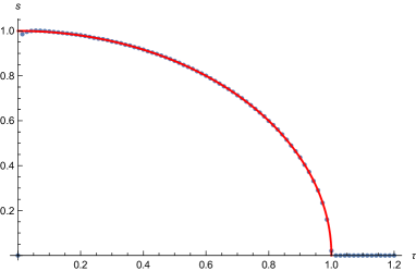
(a) $s(0,t)$

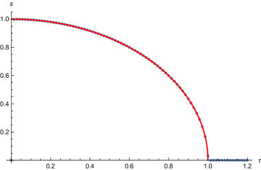
(b) $s(5,t)$

Figure 3: Plot of $s(\beta,t)$ for 3(a) $\beta=0$ and 3(b) $\beta=5$. The horizontal axis is the rescaled time $\tau=t/2N$. The blue dots are the exact values of $s(\beta,t)$ at $N=500$ while the red curve represents the semi-circle law $s=\sqrt{1-\tau^{2}}$.

In Figure 3, we plot the exact slope of ramp $s(\beta,t)$ at $N=500$ as a function of time $\tau=t/2N$. One can clearly see that $s(\beta,t)$ obeys the semi-circle law as predicted by the large $N$ analysis in the previous section. We emphasize that $s(\beta,t)$ is independent of $\beta$ in the large $N$ limit and it obeys the semi-circle law for both $\beta=0$ and $\beta\neq 0$ as shown in (33) and (35). On the other hand, $g_{\text{conn}}(\beta,t)$ itself has a non-trivial $\beta$-dependence, whose explicit form in the large $N$ limit is given by (38).

Note that the vertical and horizontal axes in Figure 2 are flipped in Figure 3. As we explained in the previous section, the $\tau$-axis corresponds to the eigenvalue density and the $s$-axis corresponds to the eigenvalues. In other words, the eigenvalue density manifests itself as the time direction in Figure 3.

As we can see from Figure 3, the slope of ramp vanishes beyond the critical value $\tau=1$, which corresponds to the so-called Heisenberg time $t_{H}=2N$ where the plateau regime sets in. This critical time is determined by the maximal value of the eigenvalue density.

5 Small $t$ behavior of the slope of ramp

In this section we will consider the small $t$ behavior of the slope of ramp $s(\beta,t)$. Since $s(\beta,t)$ is an odd function of $t$, its Taylor expansion starts from the linear term in $t$ . From the exact result of $s(\beta,t)$ at finite $N$ in (43), we can compute the coefficient of this linear term

$$s(\beta,t)=\pi e^{\frac{\beta^{2}}{N}}\left[L_{N-1}\Bigl{(}-\frac{\beta^{2}}{N}\Bigr{)}L_{N-1}^{1}\Bigl{(}-\frac{\beta^{2}}{N}\Bigr{)}-L_{N}\Bigl{(}-\frac{\beta^{2}}{N}\Bigr{)}L_{N-2}^{1}\Bigl{(}-\frac{\beta^{2}}{N}\Bigr{)}\right]t+\mathcal{O}(t^{3}).$$ (45)

In the large $N$ limit this becomes

$$s(\beta,t)=\pi\Bigl{[}I_{0}(2\beta)^{2}-I_{1}(2\beta)^{2}\Bigr{]}t+\mathcal{O}(t^{3}).$$ (46)

One can in principle compute the coefficient of $t^{3},t^{5},\cdots,$ as a function of $\beta$ using the exact result in (43). However, the computation for general $\beta$ becomes tedious when we go to higher order terms.

Instead, here we focus on the $\beta=0$ case where the higher order coefficients are easily extracted from the exact result at finite $N$ in (44)

$$s(0,t)=\frac{\pi}{2}\left[2t-2t^{3}+t^{5}+\left(-\frac{5}{18}-\frac{1}{18N^{2}}\right)t^{7}+\mathcal{O}(t^{9})\right].$$ (47)

This expansion is valid until the first and the second terms in (47) become comparable. The order of this time scale is

$$t\sim\mathcal{O}(N^{0}).$$ (48)

Summing over the order $N^{0}$ terms in (47), we find that the large $N$ limit of $s(0,t)$ in the small $t$ regime is given by the Bessel function

$$s(0,t)=\pi t\Bigl{[}J_{0}(2t)^{2}+J_{1}(2t)^{2}\Bigr{]}+\mathcal{O}(N^{-2}).$$ (49)

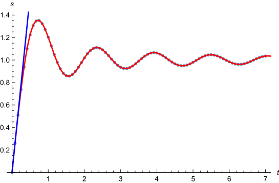
Figure 4: Plot of $s(\beta=0,t)$ in the small $t$ region. The dots are the exact values of $s(0,t)$ for $N=500$. The blue line is the first term $s=\pi t$ in the Taylor expansion of $s(0,t)$ in (47), while the red curve represents the Bessel function in (49). This figure is a closeup of the small $t$ region of Figure 3(a).

In Figure 4, we plot the exact $s(0,t)$ at $N=500$ in the small $t$ region. $s(0,t)$ grows linearly at very early time and then starts to oscillate around $s=1$. The linear behavior of $s(0,t)$ around $t=0$ comes from the first term in the Taylor expansion (47), while the oscillating behavior is captured by the Bessel function (49) as discussed in hikami .

When $t$ becomes of order $N$, the expression (49) is no longer valid; $s(0,t)$ is described instead by the semi-circle law (33) when $t\sim\mathcal{O}(N)$.

6 Conclusion

In this paper, we have studied the slope of ramp $s(\beta,t)$, which is related to $\partial_{t}g_{\text{conn}}(\beta,t)$ by (34), in the Gaussian matrix model. We found the exact closed form expression of $s(\beta,t)$ in (43) and confirmed numerically that $s(\beta,t)$ obeys the semi-circle law as a function of time for both $\beta=0$ and $\beta\neq 0$ cases. Interestingly, in the plot of $s(\beta,t)$ the time direction plays the role of eigenvalue density.

There are many interesting open questions. We list several avenues for future research. The relation between $g_{\text{conn}}$ and the eigenvalue density $\rho(\mu)$ in (22) is expected to be quite universal, and hence it is not restricted to the Gaussian matrix model. It would be very interesting to study the slope of ramp in other models, such as the SYK model, and see if the eigenvalue density manifests itself in the time direction for other models as well.

It would be also interesting to generalize our study to the higher point correlation function of $\operatorname{Tr}e^{-(\beta\pm\mathrm{i}t)H}$. In the case of Gaussian matrix model, the exact form of the connected part of higher point function was recently studied in Okuyama:2018aij . It would be interesting to see if the multi-point correlator of eigenvalues $\rho^{(n)}(\mu_{1},\cdots,\mu_{n})$ appears in the time dependence of higher point functions of $\operatorname{Tr}e^{-(\beta\pm\mathrm{i}t)H}$ in the large $N$ limit. To see this, we need to go beyond the “box approximation” used in Liu:2018hlr .

Appendix A Computation of $\operatorname{Tr}A(z)$ and $\operatorname{Tr}A(z_{1})A(z_{2})$

As discussed in Okuyama:2018aij , the correlator of $\operatorname{Tr}e^{z\sqrt{2}M}$ in Gaussian matrix model with measure $\int dMe^{-\operatorname{Tr}M^{2}}$ is easily computed by using the harmonic oscillator

$${[a,a^{\dagger}]}=1,$$ (50)

which is basically equivalent to the method of orthogonal polynomials for solving hermitian matrix models. The result is written in terms of the $N\times N$ symmetric matrix $A(z)$ with matrix element

$$A(z)_{i,j}=A(z)_{j,i}=\langle i|e^{z(a+a^{\dagger})}|j\rangle,\quad(i,j=0,\cdots,N-1),$$ (51)

where $|i\rangle$ is the orthonormal basis

$$|i\rangle=\frac{(a^{\dagger})^{i}}{\sqrt{i!}}|0\rangle,\quad\langle i|j\rangle=\delta_{i,j}.$$ (52)

Using the generating function of Laguerre polynomial

$$(1+t)^{\alpha}e^{xt}=\sum_{n=0}^{\infty}L^{\alpha-n}_{n}(-x)t^{n},$$ (53)

one can evaluate the matrix element in (51) as

$$A(z)_{i,j} =e^{-\frac{z^{2}}{2}}\langle i|e^{za}e^{za^{\dagger}}|j\rangle=\frac{1}{\sqrt{i!j!}}\partial_{s}^{i}\partial_{t}^{j}e^{-\frac{z^{2}}{2}}\langle 0|e^{(s+z)a}e^{(t+z)a^{\dagger}}|0\rangle\Bigr{|}_{s=t=0}$$ (54)

$$=\frac{1}{\sqrt{i!j!}}\partial_{s}^{i}\partial_{t}^{j}e^{-\frac{z^{2}}{2}}e^{(s+z)(t+z)}\Bigr{|}_{s=t=0}=\frac{1}{\sqrt{i!j!}}\partial_{s}^{i}e^{\frac{z^{2}}{2}+zs}(s+z)^{j}\Bigr{|}_{s=0}$$

$$=\sqrt{\frac{i!}{j!}}e^{\frac{z^{2}}{2}}z^{j-i}L_{i}^{j-i}(-z^{2}).$$

Let us first consider the trace of $A(z)$

$$\operatorname{Tr}A(z)=\sum_{i=0}^{N-1}A(z)_{i,i}=\sum_{i=0}^{N-1}\langle i|e^{z(a+a^{\dagger})}|i\rangle.$$ (55)

To evaluate this trace, it is convenient to rewrite this as a trace in the total Hilbert space $\mathcal{H}$ of harmonic oscillator

$$\operatorname{Tr}A(z)=\operatorname{Tr}_{\mathcal{H}}\bigl{(}e^{z(a+a^{\dagger})}P\bigr{)},$$ (56)

where $P$ denotes the projector to the first $N$ states

$$P=\sum_{i=0}^{N-1}|i\rangle\langle i|,$$ (57)

and $\operatorname{Tr}_{\mathcal{H}}$ is defined by

$$\operatorname{Tr}_{\mathcal{H}}O=\sum_{i=0}^{\infty}\langle i|O|i\rangle.$$ (58)

The trace on the right hand side of (56) can be simplified by using the following trick. We first notice that

$$ze^{z(a+a^{\dagger})}=[a,e^{z(a+a^{\dagger})}]=[e^{z(a+a^{\dagger})},a^{\dagger}].$$ (59)

Then, using the relation

$${[P,a]}=\sqrt{N}|N-1\rangle\langle N|,\quad{[a^{\dagger},P]}=\sqrt{N}|N\rangle\langle N-1|,$$ (60)

and the cyclicity of trace, we find

$$z\operatorname{Tr}A(z) =\operatorname{Tr}_{\mathcal{H}}[a,e^{z(a+a^{\dagger})}]P=\operatorname{Tr}_{\mathcal{H}}e^{z(a+a^{\dagger})}[P,a]$$ (61)

$$=\operatorname{Tr}_{\mathcal{H}}e^{z(a+a^{\dagger})}\sqrt{N}|N-1\rangle\langle N|=\sqrt{N}\langle N|e^{z(a+a^{\dagger})}|N-1\rangle.$$

From the explicit form of matrix element in (51) we arrive at the closed form of $\operatorname{Tr}A(z)$

$$\operatorname{Tr}A(z)=e^{\frac{z^{2}}{2}}L_{N-1}^{1}(-z^{2}).$$ (62)

Next consider the trace of the product of two $A(z)$’s

$$\operatorname{Tr}A(z_{1})A(z_{2})=\sum_{i,j=0}^{N-1}A(z_{1})_{i,j}A(z_{2})_{j,i}=\operatorname{Tr}_{\mathcal{H}}\Bigl{(}e^{z_{1}(a+a^{\dagger})}Pe^{z_{2}(a+a^{\dagger})}P\Bigr{)}.$$ (63)

One can simplify this trace using the above trick by multiplying $z_{1}+z_{2}$

$$(z_{1}+z_{2})\operatorname{Tr}A(z_{1})A(z_{2})$$ (64)

$$= \operatorname{Tr}_{\mathcal{H}}\Bigl{(}[a,e^{z_{1}(a+a^{\dagger})}]Pe^{z_{2}(a+a^{\dagger})}P+e^{z_{1}(a+a^{\dagger})}P[a,e^{z_{2}(a+a^{\dagger})}]P\Bigr{)}$$

$$= \operatorname{Tr}_{\mathcal{H}}\Bigl{(}e^{z_{1}(a+a^{\dagger})}[P,a]e^{z_{2}(a+a^{\dagger})}P+e^{z_{1}(a+a^{\dagger})}Pe^{z_{2}(a+a^{\dagger})}[P,a]\Bigr{)}$$

$$= \sqrt{N}\langle N|\Bigl{(}e^{z_{1}(a+a^{\dagger})}Pe^{z_{2}(a+a^{\dagger})}+e^{z_{2}(a+a^{\dagger})}Pe^{z_{1}(a+a^{\dagger})}\Bigr{)}|N-1\rangle.$$

The last expression can be written as a single sum of matrix elements instead of the original double sum (63)

$$(z_{1}+z_{2})\operatorname{Tr}A(z_{1})A(z_{2})$$ (65)

$$= \sqrt{N}\sum_{i=0}^{N-1}\Bigl{[}A(z_{1})_{i,N}A(z_{2})_{i,N-1}+A(z_{2})_{i,N}A(z_{1})_{i,N-1}\Bigr{]}$$

$$= e^{\frac{z_{1}^{2}+z_{2}^{2}}{2}}\sum_{i=0}^{N-1}\frac{i!}{(N-1)!}\Bigl{[}z_{1}^{N-i}z_{2}^{N-1-i}L_{i}^{N-i}(-z_{1}^{2})L_{i}^{N-1-i}(-z_{2}^{2})$$

$$\hskip 88.20354pt+z_{2}^{N-i}z_{1}^{N-1-i}L_{i}^{N-i}(-z_{2}^{2})L_{i}^{N-1-i}(-z_{1}^{2})\Bigr{]}.$$

As far as we know, there is no formula to perform this summation in a closed form. However, it turns out that the derivative of this expression can be written in a closed form.

Let us act the derivative $\partial_{1}-\partial_{2}$ on the last expression in (64) with $\partial_{k}=\frac{\partial}{\partial z_{k}}~{}(k=1,2)$. One can easily show that

$$(z_{1}+z_{2})(\partial_{1}-\partial_{2})\operatorname{Tr}A(z_{1})A(z_{2})$$ (66)

$$= \sqrt{N}\langle N|\Bigl{(}e^{z_{1}(a+a^{\dagger})}[a+a^{\dagger},P]e^{z_{2}(a+a^{\dagger})}+e^{z_{2}(a+a^{\dagger})}[P,a+a^{\dagger}]e^{z_{1}(a+a^{\dagger})}\Bigr{)}|N-1\rangle.$$

Again, using the relation (60) this is simplified as

$$(z_{1}+z_{2})(\partial_{1}-\partial_{2})\operatorname{Tr}A(z_{1})A(z_{2})$$ (67)

$$= N\Bigl{[}\langle N|e^{z_{1}(a+a^{\dagger})}|N\rangle\langle N-1|e^{z_{2}(a+a^{\dagger})}|N-1\rangle-\langle N-1|e^{z_{1}(a+a^{\dagger})}|N-1\rangle\langle N|e^{z_{2}(a+a^{\dagger})}|N\rangle\Bigr{]}$$

$$= Ne^{\frac{z_{1}^{2}+z_{2}^{2}}{2}}\Bigl{[}L_{N}(-z_{1}^{2})L_{N-1}(-z_{2}^{2})-L_{N-1}(-z_{1}^{2})L_{N}(-z_{2}^{2})\Bigr{]}.$$

By setting $z_{1}=z$ and $z_{2}=\overline{z}$ with $z,\overline{z}$ defined in (10), one can show that the above result (67) leads to the exact form of $\partial_{t}g_{\text{conn}}(\beta,t)$ in (19).