A multi-dimensional extension of the Lightweight Temporal Compression method

Abstract

Lightweight Temporal Compression (LTC) is among the lossy stream compression methods that provide the highest compression rate for the lowest CPU and memory consumption. As such, it is well suited to compress data streams in energy-constrained systems such as connected objects. The current formulation of LTC, however, is one-dimensional while data acquired in connected objects is often multi-dimensional: for instance, accelerometers and gyroscopes usually measure variables along 3 directions. In this paper, we investigate the extension of LTC to higher dimensions. First, we provide a formulation of the algorithm in an arbitrary vectorial space of dimension $n$. Then, we implement the algorithm for the infinity and Euclidean norms, in spaces of dimension 2D+t and 3D+t. We evaluate our implementation on 3D acceleration streams of human activities. Results show that the 3D implementation of LTC can save up to 20% in energy consumption for low-paced activities, with a memory usage of about 100 B.

I Introduction

With the recent technological advances in Internet of Things (IoT) applications, more than one billion connected objects are expected to be launched worldwide by 2025. Power consumption is among the biggest challenges targeting connected objects, particularly in the industrial domains, where several sensing systems are commonly launched in the field to run for days or even weeks without being recharged. Typically, such devices use sensors to capture properties such as temperature or motion, and stream them to a host system over a radio transmission protocol such as Bluetooth Low-Energy (BLE). System designers aim to reduce the rate of data transmission as much as possible, as radio transmission is a power-hungry operation.

Compression is a key technique to reduce the rate of radio transmission. While in several applications lossless compression methods are more desirable than lossy compression techniques, in the context of IoT and sensor data streams, the measured sensor data intrinsically involves noise and measurement errors, which can be treated as a configurable tolerance for a lossy compression algorithm.

Resource-intensive lossy compression algorithms such as the ones based on polynomial interpolation, discrete cosine and Fourier transforms, or auto-regression methods [1] are not well-suited for connected objects, due to the limited memory available on these systems (typically a few KB), and the energy consumption associated with CPU usage. Instead, compression algorithms need to find a trade-off between reducing network communications and increasing memory and CPU usage. As discussed in [2], linear compression methods provide a very good compromise between these two factors, leading to substantial energy reduction.

The Lightweight Temporal Compression method (LTC [3]) has been designed specifically for energy-constrained systems, initially sensor networks. It approximates data points by a piece-wise linear function that guarantees an upper bound on the reconstruction error, and a reduced memory footprint in $\mathcal{O}(1)$. However, LTC has only been described for 1D streams, while streams acquired by connected objects, such as acceleration or gyroscopic data, are often multi-dimensional.

In this paper, we extend LTC to dimension $n$. To do so, we propose an algebraic formulation of the algorithm that also yields a norm-independent expression of it. We implement our extension on Motsai’s Neblina module, and we test it on 3D acceleration streams acquired during human exercises, namely biceps curling, walking and running. Our implementation of LTC is available as free software.

We assume that the stream consists of a sequence of data points received at uneven intervals. The compression algorithm transmits fewer points than it receives. The transmitted points might be included in the stream, or computed from stream points. The compression ratio is the ratio between the number of received points and the number of transmitted points. An application reconstructs the stream from the transmitted points: the reconstruction error is the maximum absolute difference between a point of the reconstructed stream, and the corresponding point in the original stream.

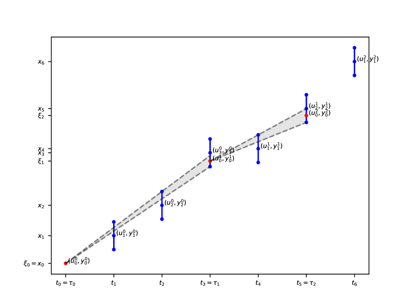
Figure 1: Illustration of the LTC algorithm. Blue dots are received points, red dots are transmitted points. Dashed lines represent the high and low lines when a point is transmitted.

Section II provides some background on the LTC algorithm, and formalizes the description initially proposed in [3]. Section III presents our norm-independent extension to dimension $n$, and Section IV describes our implementation. Section V reports on experiments to validate our implementation, and evaluates the impact of n-dimensional LTC on energy consumption of connected objects.

II Lightweight Temporal Compression

LTC approximates the data stream by a piece-wise linear function of time, with an error bounded by parameter $\epsilon$.

II-A Notations

The algorithm receives a stream of data points $x_{i}$ at times $t_{i}$ ($i\in\mathbb{N}$), and it transmits a stream of data points $\xi_{i}$ at times $\tau_{i}$ ($i\in\mathbb{N}$). To simplify the notations, we assume that:

$$\forall k\in\mathbb{N},\ \exists!i\in\mathbb{N}\ \tau_{k}=t_{i}$$

That is, transmission times coincide with reception times. We define the shifted received points as follows:

$$\forall k\in\mathbb{N}\ ,\forall j\in\mathbb{N^{*}},\ (u^{k}_{j},y^{k}_{j})=(t_{i+j},x_{i+j}),$$

where $i$ is such that $t_{i}=\tau_{k}$ and:

$$\forall k\in\mathbb{N},\ (u^{k}_{0},y^{k}_{0})=(\tau_{k},\xi_{k}).$$

This definition is such that $y^{k}_{j}$ is the $j^{th}$ data point received after the $k^{th}$ transmission and $u^{k}_{j}$ is the corresponding timestamp. Figure 1 illustrates the notations and algorithm.

The LTC algorithm maintains two lines, the high line, and the low line defined by (1) the latest transmitted point and (2) the high point (high line) and the low point (low line). When a point ($t_{i}$, $x_{i}$) is received, the high line is updated as follows: if $x_{i}+\epsilon$ is below the high line then the high line is updated to the line defined by the last transmitted point and ($t_{i}$, $x_{i}+\epsilon$); otherwise, the high line is not updated. Likewise, the low line is updated from $x_{i}-\epsilon$. Therefore, any line located between the high line and the low line approximates the data points received since the last transmitted point with an error bounded by $\epsilon$.

1:Input

2:     $(u^{k}_{j},y^{k}_{j})$      Received data stream

3:     $\epsilon$      Error bound

4:Output

5:     trTransmitted points

6:tr = $(u^{0}_{0},y^{0}_{0})$ $\triangleright$ Last transmitted point

7:k = 0 ; j = 1

8:(lp, hp) = ($y^{0}_{1}-\epsilon$, $y^{0}_{1}+\epsilon$) $\triangleright$ Low and high points

9:while True do $\triangleright$ Process received points as they come

10:     j += 1

11:     new_lp = max($y^{k}_{j}-\epsilon$, line($u^{k}_{j}$, tr, ($u^{k}_{j-1}$, lp)))

12:     new_hp = min($y^{k}_{j}+\epsilon$, line($u^{k}_{j}$, tr, ($u^{k}_{j-1}$, hp)))

13:     if new_lp $\leq$ new_hp then $\triangleright$ Keep compressing

14:         (lp, hp) = (new_lp, new_hp)

15:     else

16:         tr = $(u^{k}_{j-1},(lp+hp)/2)$ $\triangleright$ Transmit point

17:         k += 1

18:         j = 1

19:         (lp, hp) = ($y^{k}_{j}-\epsilon$, $y^{k}_{j}+\epsilon$)

20:     end if

21:end while

Algorithm 1 Original LTC algorithm, adapted from [3].

Using these notations, the original LTC algorithm can be written as in Algorithm 1. For readability, we assume that access to data points is blocking, i.e., the program will wait until the points are available. We also assume that the content of variable tr is transmitted after each assignment of this variable. Function line, omitted for brevity, returns the ordinate at abscissa $x$ (1st argument) of the line defined by the points in its 2nd and 3rd arguments.

III Extension to dimension $n$

In this section we provide a norm-independent formulation of LTC in dimension $n$. By $n$ we refer to the dimension of the data points $x_{i}$. To handle time, LTC actually operates in dimension $n+1$.

III-A Preliminary comments

We note that the formulation of LTC in [3] relies on the intersection of convex cones in dimension $n+1$. For $n=1$, it corresponds to the intersection of triangles, which can efficiently be computed by maintaining boundary lines, as detailed previously. In higher dimension, however, cone intersections are not so straightforward, due to the fact that the intersection between cones may not be a cone.

To address this issue, we formulate LTC as an intersection test between balls of dimension $n$, that is, segments for $n=1$, disks for $n=2$, etc. Balls are defined from the norm used in the vector space of data points. For $n=1$, the choice of the norm does not really matter, as all p-norms and the infinity norm are identical. In dimension $n$, however, norm selection will be critical.

III-B Algebraic formulation of LTC

III-B1 Definitions

Let $(u_{0}^{k},y_{0}^{k})\in\mathbb{R}^{n+1}$ be the latest transmitted point. For convenience, all the subsequent points will be expressed in the orthogonal space with origin $(\tau_{k},\xi_{k})$. We denote by $(v_{j},z_{j})_{j\in\llbracket 0,m\rrbracket}$ such points:

$$\forall j\leq m,\ (v_{j},z_{j})=(u_{j}^{k}-\tau_{k},y_{j}^{k}-\xi_{k})$$

Let $\mathcal{B}_{j}$ be the ball of $\mathbb{R}^{n}$ of centre $\frac{v_{1}}{v_{j}}z_{j}$ and radius $\frac{v_{1}}{v_{j}}\epsilon$:

$$\mathcal{B}_{j}=\left\{z\in\mathbb{R}^{n},\ \left\lVert z-\frac{v_{1}}{v_{j}}z_{j}\right\rVert\leq\frac{v_{1}}{v_{j}}\epsilon\right\}$$

Note that $v_{1}$ is defined as soon as one point is received after the last transmission.

III-B2 LTC property

We define the LTC property as follows:

$$\exists z\in\mathbb{R}^{n},\ \forall j\in\llbracket 1,m\rrbracket,\left\lVert\frac{v_{j}}{v_{1}}z-z_{j}\right\rVert\leq\epsilon.$$

The original LTC algorithm ensures that the LTC property is verified between each transmission. Indeed, all the data points $z$ such that $(v_{1},z)$ is between the high line and the low line verify the property. Line 13 in Algorithm 1 guarantees that such a point exists.

The LTC property can be re-written as follows:

$$\exists z\in\mathbb{R}^{n},\ \forall j\in\llbracket 1,m\rrbracket,\left\lVert z-\frac{v_{1}}{v_{j}}z_{j}\right\rVert\leq\frac{v_{1}}{v_{j}}\epsilon$$

that is:

$$\bigcap_{j=1}^{m}\mathcal{B}_{j}\neq\O$$ (1)

Note that $(\mathcal{B}_{j})_{j\in\llbracket 1,m\rrbracket}$ is a sequence of balls of strictly decreasing radius, since $v_{j}>v_{1}$.

III-C Algorithm

The LTC algorithm generalized to dimension $n$ tests that the LTC property in Equation 1 is verified after each reception of a data point. It is written in Algorithm 2.

1:Input

2:     $(u^{k}_{j},y^{k}_{j})$      Received data stream

3:     $\epsilon$      Error bound

4:Output

5:     trTransmitted points

6:tr = ($\tau,\xi$) = ($u^{0}_{0},y^{0}_{0}$) $\triangleright$ Last transmitted point

7:k = 0 ; j = 0

8:while True do

9:     j += 1

10:     ($v_{j},z_{j}$) = ($u_{j}^{k}-\tau,y_{j}^{k}-\xi$)

11:     if $\bigcap_{l=1}^{j}{\mathcal{B}_{l}}=\O$ then

12:         Pick $z$ in $\bigcap_{l=1}^{j-1}{\mathcal{B}_{j}}$ $\triangleright$ Transmit point

13:         tr = ($\tau$, $\xi$) = ($u^{k}_{j-1},z$)

14:         k += 1

15:         j = 1

16:     end if

17:end while

Algorithm 2 Generalized LTC.

III-D Ball intersections

Although Algorithm 2 looks simple, one should not overlook the fact that there is no good general algorithm to test whether a set of balls intersect. The best general algorithm we could find so far relies on Helly’s theorem which is formulated as follows [4]:

Theorem.

Let $\left\{X_{i}\right\}_{i\in\llbracket 1,m\rrbracket}$ be a collection of convex subsets of $\mathbb{R}^{n}$. If the intersection of every $n+1$ subsets is non-empty, then the whole collection has an non-empty intersection.

This theorem leads to an algorithm of complexity ${m\choose n+1}$ which is not usable in resource-constrained environments.

The only feasible algorithm that we found is norm-specific. It maintains a representation of the intersection $\bigcap_{j=1}^{m}{\mathcal{B}_{j}}$ which is updated at every iteration. The intersection tests can then be done in constant time. However, updating the representation of the intersection may be costly depending on the norm used. For the infinity norm, the representation is a rectangular cuboid which is straightforward to update by intersection with an n-ball. For the Euclidean norm, the representation is a volume with no particular property, which is more costly to maintain.

III-E Effect of the norm

As mentioned before, norm selection in $\mathbb{R}^{n}$ has a critical impact on the compression error and ratio. To appreciate this effect, let us compare the infinity norm and the Euclidean norm in dimension 2. By comparing the unit disk to a square of side 2, we obtain that the compression ratio of a random stream would be $\frac{4}{\pi}$ times larger with the infinity norm than with the Euclidean norm. In 3D, this ratio would be $\frac{6}{\pi}$. Conversely, a compression error bounded by $\epsilon$ with the infinity norm corresponds to a compression error of $\frac{\epsilon}{\sqrt{n}}$ with the Euclidean norm. Unsurprisingly, the infinity norm is more tolerant than the Euclidean norm.

It should also be noted that using the infinity norm in $\mathbb{R}^{n}$ boils down to the use of the 1D LTC algorithm independently in each dimension, since a data point will be transmitted as soon as the linear approximation doesn’t hold in any of the dimensions. For the Euclidean norm, however, the multidimensional and multiple unidimensional versions are different: the multiple unidimensional version behaves as the infinity norm, but the multidimensional version is more stringent, leading to a reduced compression rate and error.

To choose between the multidimensional implementation and multiple unidimensional ones, we recommend to check whether the desired error bound is expressed independently for every sensor, or as an aggregate error between them. The multidimensional version is more appropriate for multidimensional sensors, for instance 3D accelerometers or 3D gyroscopes, and the multiple unidimensional version is more suitable for multiple independent sensors, for instance a temperature and a pressure sensor.

IV Implementation

To implement LTC in nD with the infinity norm, we maintain a cuboid representation of $\cap_{l=1}^{j}{\mathcal{B}_{l}}$ across the iterations of the while loop in Algorithm 2. The implementation works with constant memory and requires limited CPU time.

With the Euclidean norm, the intersection test is more complex. We keep in memory a growing set $S$ of balls and the bounding box $B$ of their intersection. Then, when a new point arrives, we consider the associated ball $\mathcal{B}_{j}$ and our intersection test works as in Algorithm 3. box is a function that returns the bounding box of an n-ball. find_bisection(S, B) searches for a point in all the elements in S, using plane sweep and bisection initialized by the bounds of B. Our code is available at https://github.com/big-data-lab-team/stream-summarization under MIT license.

1:Input

2:     $S$Set of intersecting balls

3:     $B$Bounding box of the intersection of balls in $S$

4:     $\mathcal{B}_{j}$New ball to check

5:Output

6:     $S$Updated set of intersecting balls

7:     $B$Updated bounding box

8:     $T$True if all the balls in S and $\mathcal{B}_{j}$ intersect

9:if $\mathcal{B}_{j}\cap B=\O$ then $\triangleright$ Ball is outside bounding box

10:     return ($S$, $B$, False)

11:end if

12:if $\exists\ \mathcal{B}_{i}\in S$ s.t. $\mathcal{B}_{j}\cap\mathcal{B}_{i}=\O$ then

13:     return ($S$, False) $\triangleright$ Some balls don’t intersect

14:end if

15:if $\exists\ \mathcal{B}_{i}\in S$ s.t. $\mathcal{B}_{j}\subset\mathcal{B}_{i}$ then $\triangleright$ Remove inclusions

16:     Remove $\mathcal{B}_{i}$ from $B$. Add $\mathcal{B}_{j}$ to $B$.

17:end if

18:$B$ = box($\mathcal{B}_{j}$) $\ \bigcap\$ $B$

19:$S$ = $S\ \bigcup\ \{\mathcal{B}_{j}\}$

20:$x$ = find_bisection($S$, $B$) $\triangleright$ This can take some time

21:if $x$ == Null then

22:     return ($S$, $B$, False)

23:else

24:     return ($S$, $B$, True)

25:end if

Algorithm 3 Intersection test for Euclidean n-balls.

V Experiments and Results

We conducted two experiments using Motsai’s Neblina module, a system with a Nordic Semiconductor nRF52832 micro-controller, 64 KB of RAM, and Bluetooth Low Energy connectivity. Neblina has a 3D accelerometer, a 3D gyroscope, a 3D magnetometer, and environmental sensors for humidity, temperature and pressure. The platform is equipped with sensor fusion algorithms for 3D orientation tracking and a machine learning engine for complex motion analysis and motion pattern recognition [5]. Neblina has a battery of 100mAh; at 200 Hz, its average consumption is 2.52 mA when using accelerometer and gyroscope sensors but without radio transmission, and 3.47 mA with radio transmission, leading to an autonomy of 39.7 h without transmission and 28.8 h with transmission.

V-A Experiment 1: validation

Figure 2: Setup with Neblina.

We validated the behaviour of our LTC extension on a PC using data acquired with Neblina. We collected two 3D accelerometer time-series, a short one and a longer one, acquired on two different subjects performing biceps curl, with a 50 Hz sampling rate (see Figure 3). In both cases, the subject was wearing Neblina on their wrist, as in Figure 2. It should be noted that the longest time-series also has a higher amplitude, perhaps due to differences between subjects.

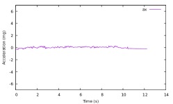
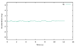
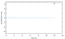
(a) Short biceps curl^a

^a Average of az data is -7.81mg. It was shifted to 0 so that the graphs can all use the same y scale.

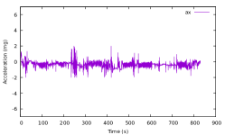
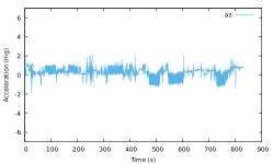
(b) Long biceps curl

Figure 3: Time-series used in Experiment 1

We compressed the time-series with various values of $\epsilon$, using our 2D (x and y) and 3D (x, y and z) implementations of LTC. On Neblina, the raw uncalibrated accelerometer data corresponds to errors around 20 mg (1 g is 9.8 m/s²). We used a laptop computer with 16 GB of RAM, an Intel i5-3210M CPU @ 2.50GHz $\times$ 4, and Linux Fedora 27. We measured memory consumption using Valgrind’s massif tool [6], and processing time using gettimeofday() from the GNU C Library.

Results are reported in Table I. As expected, the compression ratio increases with $\epsilon$, and the maximum measured error remains lower than $\epsilon$ in all cases. The maximum is reached most of the time on these time-series.

Infinity vs Euclidean norms

The average ratio between the compression ratios obtained with the infinity and Euclidean norm is 1.03 for 2D data, and 1.06 for 3D data. These ratios are lower than the theoretical values of $\frac{4}{\pi}$ in 2D and $\frac{6}{\pi}$ in 3D, which are obtained for random-uniform signals. Unsurprisingly, the infinity norm surpasses the Euclidean norm in terms of resource consumption. Memory-wise, the infinity norm requires a constant amount of 80 B, used to store the intersection of n-balls. The Euclidean norm, however, uses up to 4.7 KB of memory for the Long time-series in 3D with $\epsilon$=48.8 mg. More importantly, the amount of required memory increases for longer time-series, and it also increases with larger values of $\epsilon$. Similar observations are made for the processing time, with values ranging from 0.4 ms for the simplest time-series and smallest $\epsilon$, to 41.3 ms for the most complex time-series and largest $\epsilon$.

2D vs 3D

For a given $\epsilon$, the compression ratios are always higher in 2D than in 3D. It makes sense since the probability for the signal to deviate from a straight line approximation is higher in 3D than it is in 2D. Besides, resource consumption is higher in 3D than in 2D: for the infinity norm, 3D consumes 1.4 times more memory than 2D (1.8 times on average for Euclidean norm), and processing time is 1.35 longer (1.34 on average for Euclidean norm).

	Infinity		Euclidean
$\epsilon$ (mg)	48.8	34.5	48.8	34.5
Max error (mg)	48.8	34.4	48.8	34.5
Compression ratio (%)	79.77	72.59	77.49	70.96
Peak memory (B)	80	80	688	688
Processing time (ms)	0.101	0.094	0.456	0.406

(a) Short biceps curl (2D)

	Infinity		Euclidean
$\epsilon$ (mg)	48.8	34.5	48.8	34.5
Max error (mg)	48.8	34.5	48.8	34.5
Compression ratio (%)	77.46	70.98	75.77	68.81
Peak memory (B)	80	80	2512	2608
Processing time (ms)	6.06	5.84	33.84	31.07

(b) Long biceps curl (2D)

	Infinity		Euclidean
$\epsilon$ (mg)	48.8	28.2	48.8	28.2
Max error (mg)	48.8	28.2	48.8	28.2
Compression ratio (%)	78.14	66.39	74.39	63.13
Peak memory (B)	112	112	1744	784
Processing time (ms)	0.147	0.134	0.731	0.514

(c) Short biceps curl (3D)

	Infinity		Euclidean
$\epsilon$ (mg)	48.8	28.2	48.8	28.2
Max error (mg)	48.8	28.2	48.8	28.2
Compression ratio (%)	71.23	58.11	67.35	53.24
Peak memory (B)	112	112	4752	3856
Processing time (ms)	7.87	7.22	41.29	39.04

(d) Long biceps curl (3D)

TABLE I: Results from Experiment 1

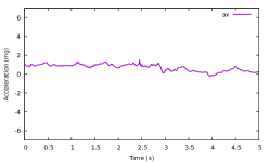
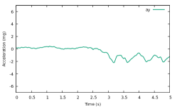
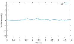
(a) Walking

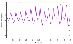
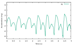
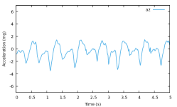
(b) Running

Figure 5: Time series used in Experiment 2

V-B Experiment 2: impact on energy consumption

We acquired two 3D accelerometer time-series at 200 Hz for two activities: walking and running (see Figure 5). In both cases, the subject was wearing Neblina on their wrist as in Experiment 1. We collected 1,000 data points for each activity, corresponding to 5 seconds of activity.

We measured energy consumption associated with the transmission of these time-series by “replaying” the time-series after loading them as a byte array in Neblina. We measured the current every 500 ms. We also measured the max and average latency resulting from compression.

Results are reported in Table II. For a given $\epsilon$ and norm, the compression ratio is larger for walking than for running. The ratio of saved energy is relative to the reference current of 3.47 mA measured when Neblina transmits data without compression. In all cases, activating compression saves energy. The reduction in energy consumption behaves as the compression ratio: it increases with $\epsilon$, it is higher for the infinity norm than for the Euclidean, and it is higher for the walking activity than for running. For a realistic error of $\epsilon$=9.8 mg, the ratio of saved energy with the infinity norm is close to 20% for the walking activity, which is substantial. Latency is higher for walking than for running, and it is also higher for the Euclidean norm than for the infinity norm. In all cases, the latency remains lower than the 5-ms tolerable latency at 200 Hz, which demonstrates the feasibility of 3D LTC compression.

	Infinity			Euclidean
$\epsilon$ (mg)	48.8	9.8	4.9	48.8	9.8	4.9
Max error (mg)	48.8	9.8	4.9	48.8	9.8	4.9
Compr. ratio (%)	88.9	66.4	45.5	87.6	63.3	37.2
Average (mA)	2.64	2.79	3.02	3.10	3.02	3.13
Saved energy (%)	23.9	19.7	13.0	10.7	13.0	9.7
Max latency ($\mu$s)	60	–	–	1530	–	–
Average latency ($\mu$s)	31	–	–	145	–	–

(a) Walking

	Infinity			Euclidean
$\epsilon$ (mg)	48.8	9.8	4.9	48.8	9.8	4.9
Max error (mg)	48.8	9.8	4.9	48.8	9.8	4.9
Compr. ratio (%)	68.6	25.5	9.5	64.4	19.8	5.7
Average (mA)	2.88	3.22	3.38	2.95	3.32	3.39
Saved energy (%)	17.0	7.2	2.5	14.9	4.3	2.2
Max latency ($\mu$s)	60	–	–	840	–	–
Average latency ($\mu$s)	30	–	–	64	–	–

(b) Running

TABLE II: Results from Experiment 2

VI Conclusion

We presented an extension of the Lightweight Temporal Compression method to dimension $n$ that can be instantiated for any distance function. Our extension formulates LTC as an intersection detection problem between n-balls. We implemented our extension on Neblina for the infinity and Euclidean norms, and we measured the energy reduction induced by compression for acceleration streams acquired during human activities.

We conclude from our experiments that the proposed extension to LTC is well suited to reduce energy consumption in connected objects. The implementation behaves better with the infinity norm than with the Euclidean one, due to the time complexity of the current algorithm to detect the intersection between n-balls for the Euclidean norm.

Our future work focuses on this latter issue. We plan to start from Helly’s theorem, which only provides an algorithm of complexity ${m\choose n+1}$ to compress $m$ points in dimension $n$. We note that Helly’s theorem holds for arbitrary convex subsets of $\mathbb{R}^{n}$, while we are considering a sequence of balls of decreasing radius. Based on this observation, a stronger result might exist that would lead to a more efficient implementation of LTC with the Euclidean norm. Our current idea is to search for a point expressed as a function of the ball centres that would necessarily belong to the ball intersection when it is not empty; such a point, if it exists, necessarily converges to the centre of the last ball in the sequence as $n$ increases, as the radius of the last ball decreases to zero. The resulting algorithm would then compute this point and check its inclusion in every ball, which is done in $\mathcal{O}(m)$ complexity.

The choice of an appropriate norm should not be underestimated. Some situations might be better described with the Euclidean norm than with the infinity norm, such as the ones involving position or movement measures. Using the infinity norm instead of the Euclidean would lead to important error differences, proportional to $\sqrt{n}$ in dimension $n$. Investigating other norms, in particular the 1-norm, would be relevant too.

References

- [1] J. Lu, F. Valois, M. Dohler, and M.-Y. Wu, “Optimized data aggregation in WSNs using adaptive ARMA,” in IEEE Conf. on Sensor Technologies and Applications, 2010, pp. 115–120.
- [2] D. Zordan, B. Martinez, I. Vilajosana, and M. Rossi, “On the performance of lossy compression schemes for energy constrained sensor networking,” ACM Transactions on Sensor Networks (TOSN), vol. 11, no. 1, p. 15, 2014.
- [3] T. Schoellhammer, E. Osterweil, B. Greenstein, M. Wimbrow, and D. Estrin, “Lightweight temporal compression of microclimate datasets,” in IEEE International Conference on Local Computer Networks, 2004, pp. 516–524.
- [4] E. Helly, “Über mengen konvexer körper mit gemeinschaftlichen punkte.” Jahresbericht der Deutschen Mathematiker-Vereinigung, vol. 32, pp. 175–176, 1923.
- [5] O. Sarbishei, “On the accuracy improvement of low-power orientation filters using IMU and MARG sensor arrays,” in IEEE International Symposium on Circuits and Systems, 2016, pp. 1542–1545.
- [6] N. Nethercote, R. Walsh, and J. Fitzhardinge, “Building workload characterization tools with valgrind,” in IEEE Symposium on Workload Characterization, 2006, pp. 2–2.