A multiple comparison procedure for dose-finding trials with subpopulations

Abstract

Identifying subgroups of patients with an enhanced response to a new treatment has become an area of increased interest in the last few years. When there is knowledge about possible subpopulations with an enhanced treatment effect before the start of a trial it might be beneficial to set up a testing strategy, which tests for a significant treatment effect not only in the full population, but also in these prespecified subpopulations. In this paper we present a parametric multiple testing approach for tests in multiple populations for dose-finding trials. Our approach is based on the MCP-Mod methodology, which uses multiple comparison procedures to test for a dose-response signal, while considering multiple possible candidate dose-response shapes. Our proposed methods allow for heteroscedasticity between populations and control the FWER over tests in multiple populations and for multiple candidate models. We show in simulations, that the proposed multi-population testing approaches can increase the power to detect a significant dose-response signal over the standard single-population MCP-Mod, when the considered subpopulation has an enhanced treatment effect.

Keywords: MCP-Mod; Multiple Testing; Subgroup Analyses; Targeted Therapies

1 Introduction

Identifying subgroups of patients with an enhanced response to a new treatment has become an area of increased interest in the last few years. Hence subgroup analyses are commonly performed all throughout the clinical development process. In many cases these analyses are performed in an exploratory fashion and a large number of possible subgroups are considered with the aim to find a patient population, in which the treatment is particularly effective. For these scenarios many novel subgroup identification and treatment effect estimation methods have been proposed see, for example, [1, 2, 3, 4, 5, 6] or [7]. An extensive overview over exploratory subgroup analysis methods is given in [8].

When such an exploratory subgroup analysis results in a promising subgroup finding, this subgroup could then be used in a future trial. Alternatively such a subgroup could be identified before the start of a trial based on clinical expert knowledge. In these situation it might be beneficial to plan the trial with the subgroup in mind and test for a treatment effect in both the full population and the subgroup. Depending on the result of the trial there are then three possible positive outcomes: (i) the drug is shown to be efficacious for all patients, (ii) the drug is shown to be efficacious only in a subgroup or (iii) the drug is shown to be efficacious for all patients but with an increased efficacy for patients in a subgroup. In the last scenario there might be uncertainty about the effect in the full population, since it could be driven by the large effect in the subgroup and the rest of the population could have negligible treatment effects. One can consider an additional test in the complement to avoid this issue.

For the design of trials, in which subpopulations are of interest, additional considerations have to be made regarding the power of the tests and possible trial designs like enrichment or adaptive designs. Some of these considerations regarding the power when testing in the whole population and a subgroup are discussed in [9] and [10]. [11] discuss several different enrichment and adaptive designs.

When tests are performed in multiple populations multiplicity has to be taken in to account to avoid an inflated type I error. It is possible to use non-parametric approaches to control multiplicity, as for example, Bonferroni or Holm-corrections, or more complex stepwise procedures as discussed in [12]. However non-parametric methods would ignore the correlations between test statistics that arise, when tests are performed in the overall population and a subgroup, where the latter is a subset of the former. Using a parametric approach can be more efficient and show an increase in power over the aforementioned methods. Such parametric approaches are for example discussed in [10] and [13].

In addition to testing in multiple populations a clinical trial might also investigate multiple doses of the same treatment. Dose-finding trials are routinely performed in Phase II of clinical development and in some cases Phase III trials also investigate several different doses of the same treatment. Frequently there might be uncertainty about the underlying dose-response shape and thus which dose-response model to fit to the data. Subgroup identification methods in the context of dose-response trials have recently been introduced in [14] and a testing approach, that can be used for dose-response-trials with a prespecified subgroup would be useful in practice as well. In this paper we want to propose such an approach, which is based on the MCP-Mod methodology ([15]).

The MCP-Mod approach combines multiple comparison procedures and modeling to analyse dose-response trials. MCP-Mod consists of two parts. In the multiple comparisons procedure (MCP) step a test for a dose-response signal is performed for several prespecified candidate dose-response shapes . The contrasts for the tests are chosen to achieve optimal power for the tests. MCP-Mod uses the joint distribution of the test statistics to control the family-wise error rate (FWER) at a specified level, while accounting for the correlations between test statistics. In case of a normally distributed outcome the joint distribution of the tests statistics is known and the correlation structure between the test statistics depends on the candidate shapes used. The more general case, which is described in [16] extends the framework to non-normal outcomes using the asymptotic distribution of the test statistics. If a dose-response signal is established under any of the considered shapes, one can continue to the second step, the modeling part. In the modeling (Mod) step significant models can then be fit to the data and be used for dose estimation. Further details concerning the design and analysis of clinical trials with MCP-Mod are discussed in [17] and [18].

The approach we propose in this paper is an extension of the MCP-part of the MCP-Mod methodology to allow for testing for a dose-response signal in multiple populations. We specifically focus on the situation of a Phase II trial, where there is uncertainty about the underlying dose-response shape and a subgroup with a possibly enhanced treatment effect has been prespecified. The proposed methods adjust for the multiplicity resulting from tests for different dose-response shapes and tests in multiple populations, and make use of the correlation between the tests. We also take into account, that variance might differ between populations. While we focus on tests in one subgroup and the full population, in general the methodology presented here can be used to perform multiple comparisons across arbitrarily overlapping populations of any number, while controlling the FWER.

The remainder of this paper is structured as follows: In the following Section we will present the methodology to perform contrast tests in multiple populations. In Section 3 we show the results of simulations, which evaluate the operating characteristics of the approach, focusing on FWER control and power. In Section 4 we summarize and discuss the results.

2 Multiple contrast tests for multiple populations

2.1 Notation, models and contrast tests

We consider a clinical trial, which has been performed in parallel groups of patients, which receive different doses $d_{1},d_{2},...,d_{k}$ of an experimental treatment. The number of patients in the dose groups are $n_{1},...,n_{k}$ and $n:=\sum\limits_{i=1}^{k}n_{i}$, the total number of patients in the study. We observe responses $\boldsymbol{Y}$, which can either be related to efficacy or safety of the new treatment. In the following we distinguish between three populations of interest: the full or overall population ($F$), which includes all patients, and two prespecified subpopulations of $F$; a subpopulation of patients, which has been identified to possibly show an enhanced treatment effect ($S$) and the complement of that subpopulation ($C$), so that $F=S\cup C$. To simplify the discussion of the methodology we introduce the two index sets, $U:=\{F,S,C\}$ and $V:=\{S,C\}$. In what follows we assume that the patients can be classified into subgroup and complement without error.

We adopt the general framework from [15], but additionally introduce the population as an additional component in the models. Analogously to the original MCP-Mod framework we therefore consider the model

$$\begin{split}Y_{ij}^{(P)}=f(d_{i},\boldsymbol{\theta})^{(P)}+\epsilon_{ij}^{(P)};\epsilon_{ij}^{(P)}\sim N(0,\sigma_{P}^{2})\hskip 14.22636pti.i.d,\\ i=1,...,k,j=1,...,n_{i}^{(P)},P\in V\end{split}$$ (1)

where $\boldsymbol{\theta}$ refers to the vector of model parameters, $i$ to the dose group and $j$ to the patient within dose group $i$ and population $P$. $n_{i}^{(P)}$ denotes the number of patients in population $P$, which are in dose group $i$, so that $n_{i}=n_{i}^{(F)}=n_{i}^{(S)}+n_{i}^{(C)}$. To simplify the discussion we assume that the prevalence of the subgroup is deterministic and constant across all dose levels. We denote the prevalence of $S$ by $\gamma:=\frac{n_{1}^{(S)}}{n_{1}^{(F)}}=\dots=\frac{n_{k}^{(S)}}{n_{k}^{(F)}}$. A more general discussion without the assumption of constant prevalences is included in the Appendix.

Model (1) is assumed to be the underlying dose-response model with regard to dose estimation. For the contrast tests, which have the aim of detecting a dose-response relationship, a different model,

$$\begin{split}Y_{ij}^{(P)}=\mu_{i}^{(P)}+\epsilon_{ij}^{(P)};\epsilon_{ij}^{(P)}\sim N(0,\sigma_{P}^{2})\hskip 14.22636pti.i.d,\\ i=1,...,k,j=1,...,n_{i}^{(P)},P\in V\end{split}$$ (2)

is considered. $\mu_{i}^{(P)}$ is the mean response for dose group $i$ in population $P$. An estimate for $\mu_{i}^{(P)}$ is the arithmetic mean $\bar{Y_{i}}^{(P)}=\sum\limits_{j=1}^{n_{i}^{(P)}}\frac{Y_{ij}^{(P)}}{n_{i}^{(P)}}$. For population $P$ we denote the vector of the estimated dose means by $\bar{\boldsymbol{Y}}^{(P)}=(\bar{Y_{1}}^{(P)},\dots,\bar{Y_{k}}^{(P)})^{{}^{\prime}}$. Additionally the pooled variance estimator for $\sigma_{P}^{2}$ is

$${S^{(P)}}^{2}=\sum\limits_{i=1}^{k}\sum\limits_{j=1}^{n_{i}^{(P)}}(Y_{ij}^{(P)}-\bar{Y_{i}}^{(P)})^{2}/\sum\limits_{i=1}^{k}(n_{i}^{(P)}-k).$$ (3)

We assume uncertainty regarding the underlying shape of the dose-response relationship and assume, that a set of plausible candidate models $\{M_{1},\dots,M_{Z}\}$ is prespecified. These models are candidates to describe the shape of the dose-response curve and produce mean vectors under the alternative. Usually candidate models are commonly encountered dose-response models like $E_{max}$, linear, exponential or quadratic shapes. These candidate models are used to obtain the contrast vectors for the tests. Contrast vectors $\boldsymbol{{c_{m}}^{{}^{\prime}}}=(c_{m1},\dots,c_{mk})$ are chosen optimally to guarantee maximal power for each single contrast test. For details on choosing the optimal contrasts see [15].

The MCP-Mod approach then tries to detect a significant dose-response relationship for at least one of the models. In theory it is possible to specify a different set of candidate shapes for each population. We assume here, that the set of candidate models is the same across all populations, which is likely plausible for most real-life situations. With this assumption and the assumption of a constant prevalence of the subgroups across all dose groups the optimal contrast vectors are independent of the population, in which the test is performed. We discuss the more general situation of different candidate models across populations in the Appendix.

For each candidate model $m\in\{M_{1},\dots,M_{Z}\}$ and each population $P\in U$ a contrast test testing the null hypothesis $H_{0}^{(P,m)}:\boldsymbol{{c_{m}}^{{}^{\prime}}\mu^{(P)}}=0$ against the alternatives $H_{1}^{(P,m)}:\boldsymbol{{c_{m}}^{{}^{\prime}}\mu^{(P)}}>0$ is performed. Using this alternative we assume without loss of generality, that the treatment effect will have a positive sign.

In total the number of tests is $3Z$. We define the population null hypothesis (in $P$) as

$$H_{0}^{(P)}:H_{0}^{(P,M_{1})}\cap...\cap H_{0}^{(P,M_{Z})},$$

the intersection of the null hypotheses for all candidate models in population $P$. The global null hypothesis is then the intersection between the population null hypotheses, in all tested populations. For example for the full testing strategy, which includes both subgroup and complement the global null hypothesis is

$$H_{0}^{(global)}:H_{0}^{(F)}\cap H_{0}^{(S)}\cap H_{0}^{(C)}$$

While rejecting the global null is of main interest, the population hypotheses have to be considered to determine if a dose-response trend has been established in all populations or, for example, only in a subgroup.

The test statistics are contrast tests of the form

$$T_{m}^{(P)}=\frac{(\boldsymbol{c_{m}})^{{}^{\prime}}\bar{\boldsymbol{Y}}^{(P)}}{\sqrt{(\hat{\sigma}^{(P)})^{2}\sum\limits_{i=1}^{k}c_{mi}^{2}/n_{i}^{(P)}}}\hskip 14.22636ptm\in\{M_{1},\dots,M_{Z}\},P\in V,$$ (4)

which are performed for each of the candidate models in each population. $(\hat{\sigma}^{(P)})^{2}$ is an estimator of the variance in population $P$. There are several estimators that could be considered. Which estimator to use depends on the assumptions made regarding possible heteroscedasticity between subgroup and complement and has an effect on the critical values used for the tests as we will discuss in the following.

If the variances in subgroup and complement are assumed to be the same, e.g. we assume homoscedasticity between populations, we can drop the population indices for the variances. Then $\sigma_{S}^{2}=\sigma_{C}^{2}=\sigma^{2}$. We can then also drop the population index from the variance estimator in (4) and use the same estimator for all tests. A pooled variances estimator (pooled over dose levels and over subgroup and complement) is the natural choice in this context, since model (2) assumes that the means are different both across dose levels, and subgroup and complement. The pooled variance estimator is then

$$\hat{\sigma}^{2}=\sum\limits_{P\in V}\sum\limits_{i=1}^{k}\sum\limits_{j=1}^{n_{i}^{(P)}}(Y_{ij}^{(P)}-\bar{Y_{i}}^{(P)})^{2}/\sum\limits_{P\in V}(\sum\limits_{i=1}^{k}n_{i}^{(P)}-k).$$ (5)

The assumption of homogeneous variances in all populations may not always be justified. For example patients in a subgroup might be assumed to be more homogeneous than patients in the full population and thus the subgroup will be assumed to have smaller variances. If we assume the variances in subgroup and complement to be unequal, e.g. we assume heteroscedasticity between subgroup and complement ($\sigma_{S}^{2}\neq\sigma_{C}^{2}$) the pooled variance estimator will generally be biased and different estimators should be used.

When heteroscedasticity is assumed, it is more appropriate to estimate the variance separately in subgroup and complement. In each population a variance estimate, which is pooled over the dose levels as in (5) can then be used. Then $(\hat{\sigma}^{(S)})^{2}=(S^{(S)})^{2}$ and $(\hat{\sigma}^{(C)})^{2}=(S^{(C)})^{2}$.

Under the global null hypothesis there is no difference between contrasts in subgroup and complement (both are assumed to be zero). Under these assumptions a weighted average of the two population variance estimates is a reasonable estimator for the variance in the full population. For the tests in the full population under assumed heteroscedasticity we would therefore use the variance estimator $(\hat{\sigma}^{(F)})^{2}=\frac{1}{n}\cdot[\sum\limits_{i=1}^{k}n_{i}^{(S)}(\hat{\sigma}^{(S)})^{2}+\sum\limits_{i=1}^{k}n_{i}^{(C)}(\hat{\sigma}^{(C)})^{2})]$.

2.2 FWER control

Performing multiple tests at once, as in the approach we described above, leads to multiplicity issues. In the classic MCP-Mod approach the family-wise error rate (FWER) across all tests is controlled, e.g. the probability to reject at least one true null hypothesis is below a specified level $\alpha$. The MCP-Mod approach makes use of the joint distribution of the test statistics to obtain critical values or adjusted $p$-values. In the situation we consider here, in addition to the multiplicity stemming from testing different candidate shapes, there is also multiplicity stemming from tests in several populations. When MCP-Mod is performed in only one population, the joint distribution is known to be multivariate $t$ under the assumptions of model (2). When considering multiple populations the joint distribution of the test statistics is only multivariate $t$, if the variance is assumed to be equal across all populations.

In the following discussion we assume that tests are performed in the full population, the subgroup and the complement, since this is the most complete testing strategy and the distributions for other strategies can easily be derived from this.

We will first consider the homoscedastic case, where variances are assumed to be equal in subgroup and complement ($\sigma_{S}^{2}=\sigma_{C}^{2}=\sigma^{2}$). Then it is appropriate to use the pooled variance estimate (5) in all populations and the vector of test statistics $\boldsymbol{T^{{}^{\prime}}}=(T_{M_{1}}^{(F)},\dots,T_{M_{Z}}^{(F)},T_{M_{1}}^{(S)},\dots,T_{M_{Z}}^{(S)},T_{M_{1}}^{(C)},\dots,T_{M_{Z}}^{(C)})$ is distributed as $MVT_{3Z}(\nu,\mathbf{0},\boldsymbol{R})$ with $\nu=\sum\limits_{P\in V}(\sum\limits_{i=1}^{k}n_{i}^{(P)}-k)$ degrees of freedom, mean vector $\mathbf{0}$ and correlation matrix $\boldsymbol{R}$. The correlation matrix has the form

$$\boldsymbol{R}=\begin{bmatrix}\boldsymbol{R_{FF}}&\boldsymbol{R_{FS}}&\boldsymbol{R_{FC}}\\ \boldsymbol{R_{FS}^{{}^{\prime}}}&\boldsymbol{R_{SS}}&\boldsymbol{R_{SC}}\\ \boldsymbol{R_{FC}^{{}^{\prime}}}&\boldsymbol{R_{SC}^{{}^{\prime}}}&\boldsymbol{R_{CC}}\\ \end{bmatrix},$$

where the entries of submatrix $\boldsymbol{R_{PQ}}\in\mathbb{R}^{Z\times Z}$ for $P,Q\in U$ are given as

$$(\rho_{ij})^{(PQ)}=\frac{\sum\limits_{l=1}^{K}c_{il}c_{jl}\cdot n_{l}^{(P\cap Q)}/(n_{l}^{(P)}n_{l}^{(Q)})}{\sqrt{\sum\limits_{l=1}^{K}{c_{il}}^{2}/n_{l}^{(P)}\sum\limits_{l=1}^{K}{c_{jl}}^{2}/n_{l}^{(Q)}}},\hskip 14.22636pti,j=1,\dots,Z.$$

Based on the above formula it is easily visible, that $\boldsymbol{R_{SC}}=\boldsymbol{0}$, since subgroup and complement are distinct. The other submatrices are easily obtainable as well, for example

$$(\rho_{ij})^{(FS)}=\sqrt{\gamma}\cdot\frac{\sum\limits_{l=1}^{k}c_{il}c_{jl}/n_{l}^{(F)}}{\sqrt{\sum\limits_{l=1}^{k}{c_{il}}^{2}/n_{l}^{(F)}\sum\limits_{l=1}^{k}{c_{jl}}^{2}/n_{l}^{(F)}}},\hskip 14.22636pti,j=1,\dots,Z$$

follows for the entries of the matrix $\boldsymbol{R_{FS}}$.

The joint distribution for performing tests only in the full population and in the subgroup without a separate test in the complement can easily be derived by dropping the irrelevant test statistics from the vector $\boldsymbol{T^{{}^{\prime}}}$ and removing the irrelevant submatrices (in this case the last row and column) from $\boldsymbol{R}$. Using the quantiles of the joint distribution as critical values for the tests will then guarantee strong control of the FWER over the population null hypotheses.

If variances cannot assumed to be equal in subgroup and complement, the situation becomes more challenging. In this case the variance estimator in the denominator of the test statistics (4) is population-dependent and the degrees of freedoms of the $t$-distributions are no longer the same in all populations. Therefore the joint distribution is not multivariate $t$ and in fact does not seem to belong to any standard probability distribution. The terms in the correlation matrix $\boldsymbol{R}$ also become more complex, since the variance terms no longer cancel out for all of the submatrices. In general the correlation submatrices then have entries

$$i,j=1,\dots,Z;P,Q\in U.$$

For example for the entries of submatrix $\boldsymbol{R_{FS}}$ we get

$$(\rho_{ij})^{(FS)}=\frac{\sigma_{S}\sum\limits_{l=1}^{K}c_{il}c_{jl}/n_{l}^{(F)}}{\sqrt{[\gamma\sigma_{S}^{2}+(1-\gamma)\sigma_{C}^{2}]\sum\limits_{l=1}^{K}{c_{il}}^{2}/n_{l}^{(F)}\sum\limits_{l=1}^{K}{c_{jl}}^{2}/n_{l}^{(S)}}},\hskip 14.22636pt\\ \ i,j=1,\dots,Z.$$

The variances $\sigma_{S}^{2}$ and $\sigma_{C}^{2}$ are usually unknown. To obtain the correlation matrix, the estimates for $\sigma_{S}^{2}$ and $\sigma_{C}^{2}$ can be plugged into the formulas above.

There are several reasonable options to approximate the joint distribution of the tests statistics under heteroscedasticity and obtain multiplicity-adjusted $p$-values. A simple solution is to assume that the variances are known and use the multivariate normal distribution to obtain $p$-values and critical values. Since the multivariate $t$ distribution approaches a multivariate normal distribution as $n\rightarrow\infty$ this approximation will work well for reasonably large sample sizes.

For small sample sizes a conservative option is to use the smallest degrees of freedom across all populations, $\nu_{min}:=\min\limits_{P\in V}\nu^{(P)}$, where $\nu^{(P)}:=\sum\limits_{i=1}^{k}n_{i}^{(P)}-k$ are the population specific degrees of freedom. In the considered setting this is equivalent to using the degrees of freedom from the population with the smallest number of patients. Then a $MVT_{3Z}(\nu_{min},\mathbf{0},\boldsymbol{R})$ - distribution can be used as an approximate joint distribution.

A less conservative approximation, which is proposed in [19] is to use a multiple degrees of freedom approximation, which translates to using a different multivariate $t$-distribution with the correct degrees of freedom for each population to obtain critical values. E.g. for test statistics from population $P\in U$, $T_{M_{1}}^{(P)},\dots,T_{M_{Z}}^{(P)}$, the critical values are obtained from a $MVT_{3Z}(\nu^{(P)},\mathbf{0},\boldsymbol{R})$ - distribution. A similar approach has also been discussed by [20] for standard (non-contrast) $t$-tests in subgroups, while additionally allowing for non-fixed sample sizes in subgroups.

Table 1 summarizes all discussed methods both under the assumption of homoscedasticity and heteroscedasticity.

Table 1: Overview over considered MCPs with the variance estimates used in the test statistics, the distribution used to obtain critical values and the degrees of freedom for the multivariate $t$ distributions. Here $\nu^{(P)}:=\sum\limits_{i=1}^{k}n_{i}^{(P)}-k$, the degrees of freedom for population $P$.

Method	Description	Variance estimation	Distribution	Degrees of freedom
SP	Standard MCP in single (full) population	pooled	multivariate $t$	$\sum\limits_{i=1}^{k}n_{i}^{(F)}-k$
MP-Pooled	Multi-population MCP assuming homoscedasticity	pooled	multivariate $t$	$\sum\limits_{P\in V}\sum\limits_{i=1}^{k}\nu^{(P)}$
MP-MinDF	Multi-population MCP assuming heteroscedasticity	population-specific	multivariate $t$ (approx.)	$\min\limits_{P\in V}\nu^{(P)}$
MP-MultDF	Multi-population MCP assuming heteroscedasticity	population-specific	multivariate $t$ (approx.)	$\nu^{(P)}$ (different for each population)
MP-Normal	Multi-population MCP assuming heteroscedasticity	population-specific	multivariate normal (approx.)	-

3 Simulation study

In this section we discuss results of a simulation study to evaluate the properties of the multi-population testing approaches. The simulation setup is similar to the one used in [15]. The simulations are divided into two main parts. In the first part (Section 3.2) we assume homoscedasticity across populations and evaluate the power of the proposed multi- population testing approaches compared to the standard single population MCP, which only considers the full population. The second part (Section 3.3) deals with the scenario of heteroscedastic populations. In addition to the comparison of multi-population MCP to single population MCP the main focus of this Section is to evaluate the different considered procedures, which are based on approximations of the joint distribution, with regard to FWER control and power.

3.1 Simulation setup

We simulate clinical trials with parallel groups, which are balanced over the dose levels. In our simulated trial patients are randomized to one of five different dose groups with dose levels 0, 0.05, 0.2, 0.6, 1. We assume that there is knowledge about a subgroup, which possibly shows an enhanced treatment effect and could have been identified from an earlier trial or based on the mode of action of the drug. We also make the simplifying assumption, that for each dose group the proportion of patients in the subgroup is equal. Together with the assumption of a balanced trial design, this means, that $n_{1}^{(S)}=\dots=n_{k}^{(S)}$.

We generate the observed data for the simulated trials from models of the form

$$\begin{split}Y_{ij}^{(P)}=f(d_{i},\boldsymbol{\theta})^{(P)}+\epsilon_{ij}^{(P)};\epsilon_{ij}^{(P)}\sim N(0,\sigma_{P}^{2})\hskip 14.22636pti.i.d,\\ i=1,...,k,j=1,...,n_{i}^{(P)},P\in V\end{split}$$ (6)

and use common dose-response shapes for $f$. An overview over the used dose-response shapes is given in Table 2. We also include a constant model to generate data under the global null hypothesis.

Table 2: Data generating dose-response models and corresponding standardized versions, which are used as candidate shapes to determine optimal contrast tests. Parameters specified in the last column are fixed for all simulated trials and are used as guesstimates to derive optimal contrasts.

Model	$f(d,\boldsymbol{\theta})$	standardized model	fixed parameters
Constant	0.2	-	-
Emax	$\theta_{0}+\frac{\theta_{1}d}{(\theta_{2}+d)}$	$\frac{d}{(\theta_{2}+d)}$	$\theta_{0}=0.2$; $\theta_{2}=0.2$
Linear	$\theta_{0}+\theta_{1}d$	$d$	$\theta_{0}=0.2$
Exponential	$\theta_{0}+\theta_{1}\cdot exp[\frac{d}{\theta_{2}}-1]$	$exp[\frac{d}{\theta_{2}}-1]$	$\theta_{2}=0.29$
Logistic	$\theta_{0}+\frac{\theta_{1}}{1+exp[(\theta_{2}-d)/\theta_{3}}$	$\frac{1}{1+exp[(\theta_{2}-d)/\theta_{3}}$	$\theta_{2}=0.4$; $\theta_{3}=0.091$
Quadratic	$\theta_{0}+\theta_{1}d+\theta_{2}d^{2}$	$d+\frac{\theta_{2}}{\lvert\theta_{1}\rvert}d^{2}$	$\frac{\theta_{1}}{\theta_{2}}=1.171$

The subgroup we simulate has prevalences $\gamma$ of either 0.25, 0.5 or 0.75. We assume that the underlying shape is the same for subgroup and complement. However the ’slope’ parameters of the model, which are not fixed (see Table 2) can vary between populations. This allows us to simulate scenarios with different treatment effects between subgroup and complement.

We consider three scenarios for how the treatment effect is distributed between subgroup and complement. In the first scenario there is no enhanced effect in the subgroup, e.g. the treatment effect is identical in the subgroup and the complement (same-scenario). In the second scenario the treatment effect in the subgroup is double the size of the effect in the complement (double-scenario). Finally for the third and last scenario there is only a treatment effect in the subgroup and the treatment effect in the complement is zero (only-scenario). The three different scenarios represent situations, in which there is in reality no subgroup and possible treatment effects are constant across the full population (same) , or in which a treatment effect in the full population is driven mostly (double) or completely (only) by a large effect in the subgroup.

We choose the (non-fixed) parameters for the non-constant models, so that the treatment effect at the highest dose is 0.6, which leads to a power of 80% (for a pairwise comparison) for a group size of 75. For the same-scenario 0.6 is the treatment effect in the full population, for the only- and double-scenarios it is the treatment effect in the subgroup. This leads to scenarios, where the treatment effect is relatively large in the subgroup but possibly hard to detect (depending on $\gamma$) in the full population.

For the multiple comparison procedure we then perform tests for all non-constant shapes in Table 2 in all populations we consider, irrespective of which of the shapes was used for data-generation. For the multi-population MCP approaches we compare two different testing strategies. These testing strategies differ with regards to the populations in which tests are performed. Tests are performed either in the full population and the subgroup ($F+S$) or in full population, subgroup and the complement ($F+S+C$). The first strategy would be used in a situation, where there is information about a possibly existing subgroup, which could potentially have an enhanced treatment effect. The second strategy could be applied in a similar situation, but could additionally be used to confirm that the treatment effect in the full population is not only driven by a subgroup with an enhanced effect. If the test could also be rejected in the complement then this would confirm that there is consistency across the whole population with regards to the treatment effects.

3.2 Homoscedastic scenarios

We will first discuss the simulation results for equal variances in subgroup and in the complement. For these simulations we fix the standard deviations at $\sigma_{S}=\sigma_{C}=1.478$. The results discussed in this Section are based on 5000 simulated trials. In the article only selected results are shown. Complete simulation results for all data-generating models are included in the Supporting Information.

In the homoscedastic case the exact joint distributions of the test statistics can be used to obtain critical values or adjusted $p$-values for the individual tests as described in Section 2.2. Since the exact distribution of the tests statistics is known, FWER is controlled at the nominal $5\%$-level for all testing methods, when data are generated under the global null hypothesis, from a constant model. This is confirmed in the simulation results, when data are generated from a constant model (shown in Supporting Information).

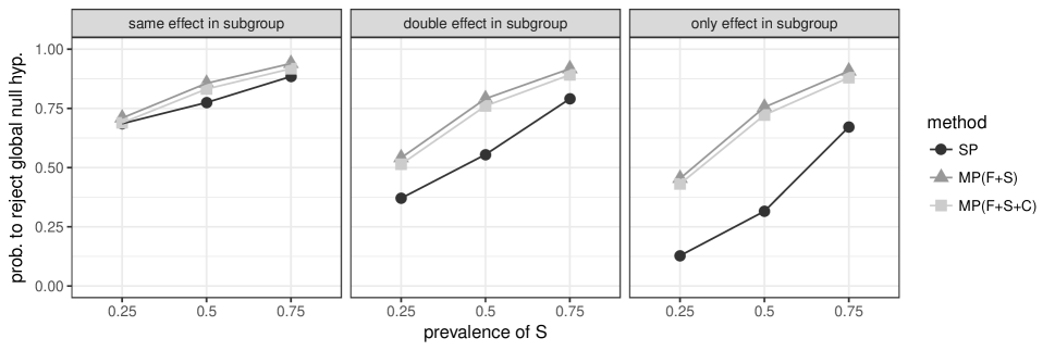
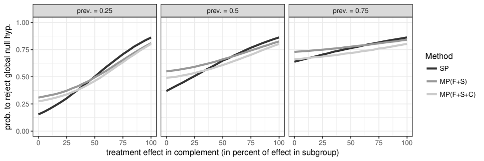
When we simulate data under the alternative of an existing dose-response trend, the MP testing approach with tests in full population and subgroup increases the chance of rejecting the global null hypothesis, when the treatment effect only exists in the subgroup or is doubled in the subgroup. This is visualized for data generated from an $E_{max}$ model in Figure 1. The MP approach with tests in all populations (F + S + C) also shows more rejections than SP in the only-scenario. In the same-scenario SP rejects most often, but the loss in power for the MP methods is relatively small, especially when the subgroup is large.

Figure 1: Probability to reject the global null hypothesis for single population (SP) and multi-population (MP) testing methods. Data are generated from an $E_{max}$ model under homoscedasticity.

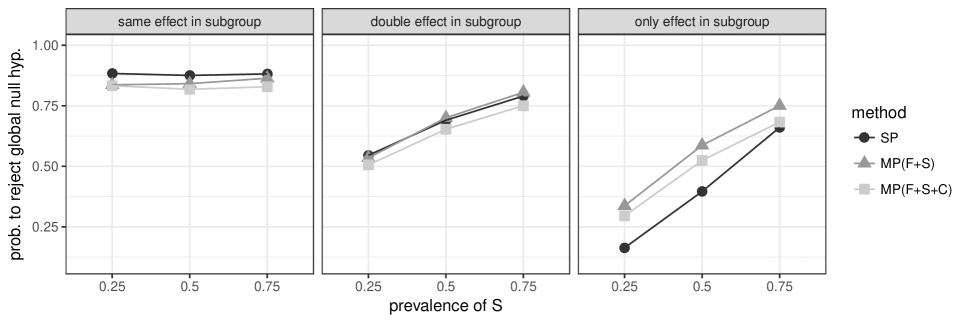
For the MP methods it might additionally be of interest, for which population(s) a significant dose-response relationship is declared. For example a significant result only in the subgroup, but not in the full population or the complement might lead to very different conclusions than significant results in all populations. Population specific rejection results for data generated from $E_{max}$ models are summarized in Table 3. The results show that when the treatment effect only exists in the subgroup, the null hypothesis in the subgroup is rejected up to $24\%$ more often than the null hypothesis in the full population. The null hypothesis for the complement, which is true in the only-scenario is only rejected in $2\%$ of simulations. When the treatment effect in the subgroup is doubled over the complement rejections generally occur more often in the full population than in the subgroup. The difference decreases with increasing subgroup prevalence $\gamma$. Table 3 also includes the results for the MP-MultDF method, which would also allow for possible heteroscedasticity. The results are essentially the same as for MP-Pooled, there does not seem to be a big penalty for allowing for heteroscedasticity in homoscedastic scenarios.

Table 3: Probability to reject the global null hypothesis and population null hypotheses for single population (SP) and multi-population (MP) testing methods. Data are generated from an $E_{max}$ model under homoscedasticity.

		Scenario and Prevalence
		same	same	same	double	double	double	only	only	only
Method	Hypothesis	0.25	0.5	0.75	0.25	0.5	0.75	0.25	0.5	0.75
SP	global	0.88	0.88	0.88	0.55	0.69	0.79	0.16	0.40	0.66
MP-Pooled(F+S)	global	0.84	0.84	0.86	0.54	0.70	0.81	0.34	0.59	0.75
	F	0.82	0.82	0.85	0.44	0.60	0.74	0.11	0.31	0.60
	S	0.31	0.55	0.73	0.30	0.54	0.73	0.30	0.55	0.72
MP-Pooled(F+S+C)	global	0.83	0.82	0.83	0.51	0.65	0.75	0.30	0.52	0.68
	F	0.79	0.77	0.79	0.40	0.55	0.67	0.09	0.26	0.53
	S	0.28	0.47	0.66	0.27	0.48	0.67	0.26	0.49	0.65
	C	0.65	0.47	0.27	0.21	0.15	0.08	0.02	0.02	0.02
MP-MultDF(F+S)	global	0.83	0.84	0.87	0.53	0.69	0.80	0.35	0.59	0.76
	F	0.81	0.82	0.85	0.42	0.59	0.74	0.12	0.32	0.60
	S	0.28	0.53	0.72	0.30	0.54	0.73	0.30	0.55	0.72
MP-MultDF(F+S+C)	global	0.83	0.82	0.83	0.49	0.64	0.75	0.31	0.53	0.69
	F	0.78	0.77	0.79	0.38	0.53	0.67	0.10	0.27	0.52
	S	0.25	0.47	0.65	0.26	0.47	0.66	0.27	0.48	0.64
	C	0.65	0.47	0.26	0.20	0.14	0.08	0.02	0.02	0.02

One of the main features of the discussed methods is the possibility to test for several possible dose-response shapes. Hence it is also of interest to compare the model selection performance of the MP testing approaches compared to the SP-MCP. Table 5 in the appendix shows the probability of choosing the correct model for the different methods. The probability of choosing the correct model based on the lowest significant $p$-value is almost identical between SP and MP approaches and therefore testing in multiple populations does not seem to reduce the model selection performance.

3.3 Heteroscedastic scenarios

In this part we will show simulation results, when testing in multiple populations with different variances. Here we use $\sigma_{S}=1.03$ and $\sigma_{C}=1.926$ for the standard deviations in subgroup and complement. The combined standard deviation in the full population thus remains the same as before at 1.478, as long as subgroup and complement have equal prevalence ($\gamma=0.5$).

As discussed in Section 2.2 the joint distribution of the contrast test statistics does not follow a standard distribution, when variances are heterogeneous and instead approximations to the true joint distribution are necessary to obtain critical values. In these simulations we will therefore first compare the different possible approximations we discuss in Section 2.2. We focus on FWER control and power for the considered approximations. For these simulations we increased the number of simulations from 5000 to 25000, to ensure that possible differences between the methods are distinguishable from simulation error.

The approaches we consider for approximating the joint distribution are MP-MinDF, MP-MultDF and MP-Normal (see Table 1). All of these approaches use separate variance estimates for the tests in subgroup and complement. To evaluate the general necessity of using population-specific variance estimates we also include test statistics using the pooled variance estimate (MP-Pooled), which assumes, that variances are the same in subgroup and complement.

Figure 2 shows the probability of rejecting the global null hypothesis when the global null is true, e.g. data are generated from a constant model. MP-Pooled, which ignores heteroscedasticity, generally does not control the FWER at the nominal level, since the variance in the complement is underestimated, when the subgroup is large. For a subgroup with prevalence of 0.75 the FWER is generally above 0.1 with the pooled variance estimate. Of the three approximations, which use population-specific variance estimates, MP-Normal is as expected liberal and leads to a large inflation of the FWER for small sample sizes. For large sample sizes MP-Normal approximates the true joint distribution better and the FWER is close to the nominal level. Of the two remaining approaches, which use approximate multivariate $t$ distributions, the MP-MinDF approach controls the FWER rate at the nominal level for all sample sizes and prevalences. MP-MultDF shows similar error rates but shows FWERs slightly higher than 0.05 for very small sample sizes.

Figure 2: Probability to reject the global null hypothesis for different multi-population (MP) testing methods. Data are generated from a constant model under heteroscedasticity. Tests were performed in full population, subgroup and complement. Bars show the $95\%$ - confidence intervals (accounting for simulation error).

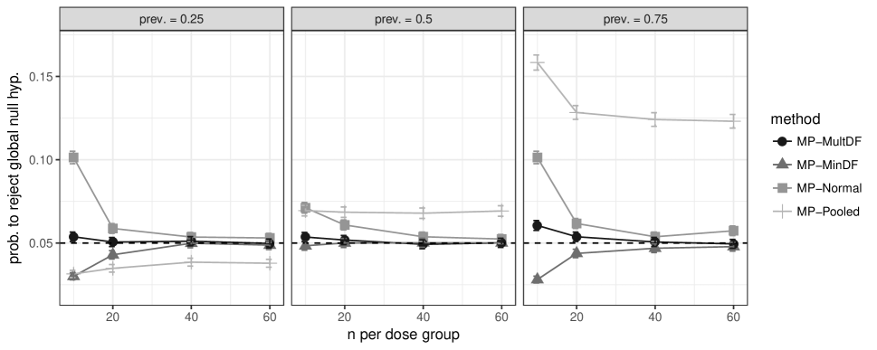
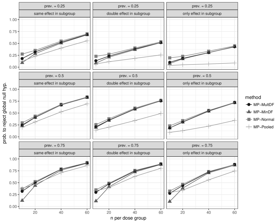
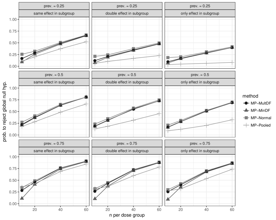
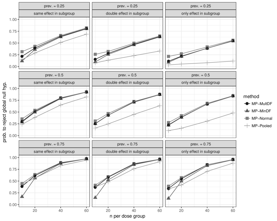
Figure 3 visualizes the differences with regards to power, e.g. the frequency of rejections of the global null hypothesis for data generated from an $E_{max}$ model for different scenarios and subgroup prevalences. With pooled variance estimation the power is generally reduced compared to the other methods. The approaches using population-specific variances estimates show fairly similar power, with MP-Normal being more liberal for small sample sizes and therefore rejecting more often. The MP-MultDF approach always leads to slightly more rejections than the MP-MinDF approach. The conclusions for the other data-generating dose-response models are similar, detailed results for these models can be found in the Supporting Information.

Figure 3: Probability to reject the global null hypothesis for different multi-population (MP) testing methods. Data are generated from an $E_{max}$ model under heteroscedasticity. Tests were performed in full population, subgroup and complement.

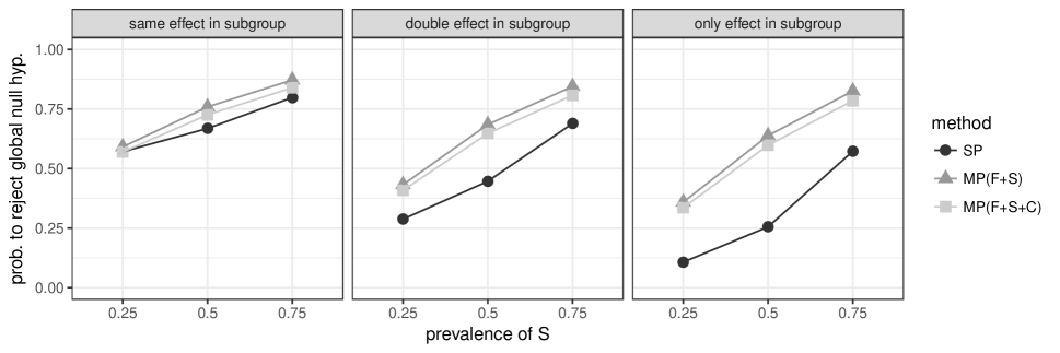
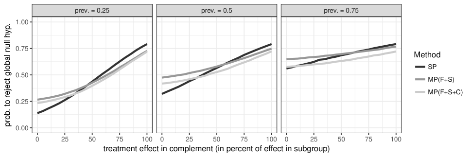
Finally it is of interest to compare the multi-population testing strategies to the single population MCP in the heteroscedastic setting as well. We focus here on the MP-MultDF approach, since it gives FWER control roughly at the nominal level, while not sacrificing too much power. Figure 4 compares the methods for a sample size of 60 per group. Comparing Figure 4 to Figure 1 the differences are now even larger between SP and MP methods. Since SP does not account for the different variances in subgroup and complement, the MP methods give better power even when there is no increased treatment effect in the subgroup and the treatment effect is the same for all patients.

Figure 4: Probability to reject the global null hypothesis for single population (SP) and multi-population (MP) testing methods. Data are generated from an $E_{max}$ model under heteroscedasticity. MP-MultDF is used to approximate the joint distribution for MP testing methods.

4 Discussion

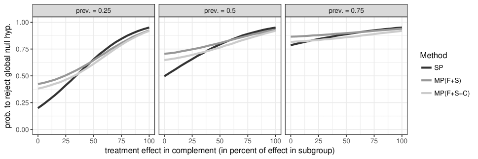
In this paper we discussed an extension of the MCP part of the MCP-Mod methodology to allow for testing in multiple populations. We focused on the situation of a dose-response trial, where a subgroup with a suspected enhanced treatment effect has been prespecified. Our method allows for simultaneous testing in full population, subgroup and possibly complement under model uncertainty, while controlling the FWER across all candidate models and populations. Our simulation results in Section 3.2 and 3.3 show, that an increase in power of rejecting the global null hypothesis can be achieved, when using the multi-population approach. The results suggest, that the prevalence of the subgroup and the size of the treatment effect in the subgroup relative to the complement are important factors to determine if a multi-population approach is worth considering. Additional plots, which visualize the effects of these factors on the power in more detail are included in the Supporting Information.

Instead of considering the power, one can also use sample size calculations to illustrate the potential benefits of a multi-population testing approach. Table 4 shows the sample sizes needed to achieve $80\%$ power for rejecting the global null hypothesis under the scenarios considered for the simulation study in Section 3. For situations, where the subgroup has a strongly enhanced effect over the rest of the population, the sample sizes for the trial can be significantly reduced when using a multi-population approach instead of a single-population approach.

Table 4: Sample sizes (per dose) required to achieve $80\%$ power for rejecting the global null hypothesis for single population (SP) and multi-population (MP) testing methods. Required sample sizes are calculated under the assumption of homoscedasticity across populations.

	Scenario and Prevalence
	same	same	same	double	double	double	only	only	only
Method	0.25	0.5	0.75	0.25	0.5	0.75	0.25	0.5	0.75
SP	59	60	59	151	105	77	932	235	105
MP-Pooled(F+S)	70	67	63	151	101	75	275	131	84
MP-Pooled(F+S+C)	71	70	70	163	112	87	299	147	97

In the heteroscedastic case, the simulation results discussed in 3.3 show, that the multiple degrees of freedom approach seems to result in a good approximation to the joint distribution of the test statistics. The FWER-inflation is minimal compared to the multivariate normal approximation, which is only suitable for large sample sizes. Additionally, the multiple degrees of freedom approach sacrifices less power than the conservative minimum degrees of freedom approach.

In the introduction we stated three different outcomes for a trial in multiple populations: (i) the drug is shown to be efficacious for all patients, (ii) the drug is shown to be efficacious only in a subgroup or (iii) the drug is shown to be efficacious for all patients but with an increased efficacy for patients in a subgroup. The methodology we present here can be used to help with decision-making in this context. We would advise to use our methodology together with estimates of treatment effects in the different populations to decide which of the three outcomes is achieved. [21] propose a decision framework for testing in a subgroup and the full population to arrive at one of the three conclusions.

We focused on scenarios, where a single subgroup and possibly the complement were considered for testing apart from the full population. Nevertheless the methodology we present here is not restricted to this setting and can be used to test in an arbitrary number of populations. We extend the method to more general scenarios in the Appendix in Section A.1. While one could therefore include a large number of subgroups and use the presented methodology to identify subgroups with an enhanced effect, we would like to point out that in contrast to other subgroup identification approaches our method does not test for an interaction between subgroup and treatment. A significant result in a subgroup does therefore not necessarily indicate, that the subgroup shows a differential effect and could be caused by a treatment effect, that is large but constant across all populations. Still, there are certain outcomes, which can be indicative of a subgroup with a larger treatment effect, most notably, when the population null hypothesis for the subgroup is rejected but the population null hypothesis for the full population is not. In our simulations this can be seen for some scenarios in Table 3. For scenarios, where there is only an effect in the subgroup, the null hypothesis for the subgroup is more often rejected than for the full population.

We only consider normally distributed outcomes in this article. The MCP-Mod methodology has been generalized to other types of outcomes in [16]. It is possible to apply the presented methodology to general parametric models. In the general case of MCP-Mod the approximate multivariate normal distribution is used. We already use this approximation in this article in Section 3.3 and show that it is a reasonable approximation for large sample sizes. The correlation matrices we discuss in Section 2.2 can simply be used for the multivariate normal instead of the multivariate $t$ in the general case.

The testing procedure discussed here is a single-step test. Alternatively a sequentially rejective test using the closed testing principle could be used as well. A similar procedure is discussed for the single-populaton MCP-Mod in [22]. Furthermore, similarly as in [13], the multiple testing procedure can be generalized to a weighted test and extended to a graph-based closed testing procedure.

The approach we present here only extends the MCP-part of MCP-Mod to multiple populations, ignoring the modeling part. In the standard MCP-Mod either the dose-response model with the lowest $p$-value is used for dose estimation or all significant models are combined via model averaging. Similar solutions in the multi-population scenario could be fitting the model with an interaction term for the subgroup, if the subgroup is significant, or using a model averaging approach that also includes subgroups, as for example discussed in [23]. Extending the modeling part of the methodology to trials with multiple populations therefore remains as an area for further research.

Appendix

A.1. Joint distribution in the general case

In this Section we derive the correlation matrix for the joint distribution of the contrast tests. We will derive the matrix for a general case with an arbitrary number of populations and also include the possibility that different candidate shapes are tested in each population. The scenarios described in 2.2 are special cases of what we discuss in this Section.

We assume that we have $W$ populations that we consider for testing. These populations are contained in the family $U:=\{P_{1},\dots,P_{W}\}$, where each population $P\in U$ is a set of patients, so that $P\subset\{1,\dots,n\}$. As in the main part of the article we need to introduce a second family of pairwise disjoint populations $V:=\{P_{1}^{*},\dots,P_{W^{*}}^{*}\}$, so that $\bigcup\limits_{r=1}^{W^{*}}P_{r}^{*}=\{1,\dots,n\}$, if we want to allow for populations with different variances. We then assume that our responses come from the model

$$\begin{split}Y_{ij}^{(P^{*})}=\mu_{i}^{(P^{*})}+\epsilon_{ij}^{(P^{*})};\epsilon_{ij}^{(P^{*})}\sim N(0,\sigma_{P^{*}}^{2})\hskip 14.22636pti.i.d,\\ i=1,...,k,j=1,...,n_{i}^{(P^{*})},P^{*}\in V\end{split}$$ (7)

and the vector of responses is $\boldsymbol{Y}=(Y_{11},...,Y_{1n_{1}},...,Y_{K1},...,Y_{Kn_{K}})$ with $Cov(\boldsymbol{Y}):=\boldsymbol{\Sigma_{Y}}$. We therefore allow each population in $V$ to have a different variance. We need to make the distinction between $V$ and $U$, since the populations in $U$ need not necessarily be pairwise disjoint. For example in the main article, subgroup and complement are in both families but the full population is only in $U$.

We now assume that in each population $P\in U$ we test for $Z_{P}$ different candidate shapes. In each population P we therefore perform tests of $H_{0}^{(P,m)}:{c_{m}^{(P)}}^{{}^{\prime}}\boldsymbol{\mu^{(P)}}=0$ against the alternatives $H_{1}^{(P,m)}:{c_{m}^{(P)}}^{{}^{\prime}}\boldsymbol{\mu^{(P)}}>0$, for $m=1,\dots,Z_{P}$. The test statistics for these hypotheses are then

$$T_{m}^{(P)}=\frac{(\boldsymbol{c_{m}^{(P)}})^{{}^{\prime}}\bar{\boldsymbol{Y}}^{(P)}}{\sqrt{(\hat{\sigma}^{(P)})^{2}\sum\limits_{i=1}^{k}\boldsymbol{c_{m}^{(P)}}^{2}/n_{i}^{(P)}}}\hskip 14.22636pt,$$ (8)

where $\bar{\boldsymbol{Y}}^{(P)}$ is the vector of the estimated means on each dose level $\boldsymbol{\bar{Y}^{(P)}}=(\bar{Y_{1}}^{(P)},...,\bar{Y_{k}}^{(P)})^{{}^{\prime}}$ and $(\hat{\sigma}^{(P)})^{2}$ the estimated variances.

For the joint distribution of the test statistics we need to derive the correlation matrix of the vector

$$\boldsymbol{T^{*}:=[(c_{1}^{(P_{1})})^{{}^{\prime}}\bar{Y}^{(P_{1})},\dots,(c_{Z_{P_{1}}}^{(P_{1})})^{{}^{\prime}}\bar{Y}^{(P_{1})},\dots,(c_{1}^{(P_{W})})^{{}^{\prime}}\bar{Y}^{(P_{W})},\dots,(c_{Z_{P_{W}}}^{(P_{W})})^{{}^{\prime}}\bar{Y}^{(P_{W})}]^{{}^{\prime}}}$$

We denote by $\Gamma_{P}:=[\boldsymbol{c_{1}^{(P)}},...,\boldsymbol{c_{Z_{P}}^{(P)}}]$ the matrix of optimal contrast coefficients for population $P$ and by $A_{P}\in\mathbb{R}^{kxn}$ a matrix with entries

$$(a_{ij})=\begin{cases}\frac{1}{n_{i}^{(P)}}&\text{if the j-th patient is on dose i and is in population P}\\ 0&\text{else}\end{cases},$$

so that $\boldsymbol{A_{P}}\boldsymbol{Y}=\bar{\boldsymbol{Y}}^{(P)}$. We can then write the required covariance matrix between all contrasts as

$$\boldsymbol{Cov(T^{*})=Cov\left(\begin{bmatrix}\Gamma_{P_{1}}^{{}^{\prime}}&\huge 0&\huge 0\\ \huge 0&\ddots&\huge 0\\ \huge 0&\huge 0&\boldsymbol{\Gamma}_{P_{W}}^{{}^{\prime}}\end{bmatrix}\begin{bmatrix}\bar{Y}^{(P_{1})}\\ \vdots\\ \bar{Y}^{(P_{W})}\end{bmatrix}\right)=Cov\left(\begin{bmatrix}\Gamma_{P_{1}}^{{}^{\prime}}&\huge 0&\huge 0\\ \huge 0&\ddots&\huge 0\\ \huge 0&\huge 0&\Gamma_{P_{W}}^{{}^{\prime}}\end{bmatrix}\begin{bmatrix}A_{P_{1}}\\ \vdots\\ A_{P_{U}}\end{bmatrix}Y\right)=}$$

$$\boldsymbol{\begin{bmatrix}\Gamma_{P_{1}}^{{}^{\prime}}A_{P_{1}}\\ \vdots\\ \Gamma_{P_{W}}^{{}^{\prime}}A_{P_{W}}\end{bmatrix}\Sigma_{Y}\begin{bmatrix}\Gamma_{P_{1}}^{{}^{\prime}}A_{P_{1}}\\ \vdots\\ \Gamma_{P_{W}}^{{}^{\prime}}A_{P_{W}}\end{bmatrix}^{{}^{\prime}}=\begin{bmatrix}\Gamma_{P_{1}}^{{}^{\prime}}A_{P_{1}}\Sigma_{Y}A_{P_{1}}^{{}^{\prime}}\Gamma_{P_{1}}^{{}^{\prime}}&\ldots&\Gamma_{P_{1}}^{{}^{\prime}}A_{P_{1}}\Sigma_{Y}A_{P_{W}}^{{}^{\prime}}\Gamma_{P_{W}}^{{}^{\prime}}\\ \vdots&\ddots&\vdots\\ \Gamma_{P_{W}}^{{}^{\prime}}A_{P_{W}}\Sigma_{Y}A_{P_{1}}^{{}^{\prime}}\Gamma_{P_{1}}^{{}^{\prime}}&\ldots&\Gamma_{P_{W}}^{{}^{\prime}}A_{P_{W}}\Sigma_{Y}A_{P_{W}}^{{}^{\prime}}\Gamma_{P_{W}}^{{}^{\prime}}\\ \end{bmatrix}}:=$$

$$\boldsymbol{\begin{bmatrix}\Sigma_{P_{1}P_{1}}&\ldots&\Sigma_{P_{1}P_{W}}\\ \vdots&\ddots&\vdots\\ \Sigma_{P_{W}P_{1}}&\ldots&\Sigma_{P_{W}P_{W}}\\ \end{bmatrix}.}$$

From this covariance matrix we can obtain the required correlation matrix $\boldsymbol{R}$.

$$\boldsymbol{R=\begin{bmatrix}R_{P_{1}P_{1}}&\ldots&R_{P_{1}P_{W}}\\ \vdots&\ddots&\vdots\\ R_{P_{W}P_{1}}&\ldots&R_{P_{W}P_{W}}\\ \end{bmatrix}},$$

where the entries of the submatrix $\boldsymbol{R_{PQ}}$ for the correlations between tests in populations $P$ and $Q$ are

$$(\rho_{ij})^{(PQ)}=\frac{\sum\limits_{l=1}^{K}[c_{il}c_{jl}/(n_{l}^{(P)}n_{l}^{(Q)})\sum\limits_{P^{*}\in V}n_{l}^{(P\cap Q\cap P^{*})}\sigma_{P^{*}}^{2}]}{\sqrt{\sum\limits_{l=1}^{K}[{c_{il}}^{2}/{n_{l}^{(P)}}^{2}\sum\limits_{P^{*}\in V}n_{l}^{(P\cap P^{*})}\sigma_{P^{*}}^{2}]\sum\limits_{l=1}^{K}[{c_{jl}}^{2}/{n_{l}^{(Q)}}^{2}\sum\limits_{P^{*}\in V}n_{l}^{(Q\cap P^{*})}\sigma_{P^{*}}^{2}}]}.$$

The cases discussed in the main part of this article correspond to $U=\{F,S,C\}$ and $V=\{S,C\}$.

As in the main part of the article the form of the joint distribution, which is used to derive critical values depends on the variance estimators in (8). Possible joint distributions are summarized in Table 1. In the general case the degrees of freedom have to be adjusted for the possible higher number of populations as well.

A.2. Simulation results for model selection

Table 5 shows the simulation results for model selection in the case of homogeneous variances in subgroup and complement. The Table shows the probability of choosing the correct model as the best model in the MCP-step. The best model is defined as the model with the lowest $p$-value over all tested populations.

Table 5: Probability of choosing the correct dose-response model for single population (SP) and multi-population (MP) testing methods. The best model is chosen based on the lowest significant $p$-value across all populations. Probabilities shown are conditional on the global null hypothesis being rejected.

		Scenario and Prevalence
		same	same	same	double	double	double	only	only	only
Correct model	Method	0.25	0.5	0.75	0.25	0.5	0.75	0.25	0.5	0.75
emax	SP	0.50	0.51	0.50	0.37	0.44	0.45	0.26	0.33	0.40
	MP-Pooled(F+S)	0.49	0.49	0.48	0.38	0.44	0.45	0.34	0.40	0.45
	MP-Pooled(F+S+C)	0.48	0.48	0.49	0.37	0.43	0.46	0.34	0.41	0.46
linear	SP	0.27	0.28	0.27	0.17	0.21	0.24	0.10	0.16	0.21
	MP-Pooled(F+S)	0.27	0.27	0.27	0.17	0.21	0.24	0.18	0.20	0.24
	MP-Pooled(F+S+C)	0.27	0.28	0.27	0.17	0.20	0.24	0.19	0.20	0.24
exponential	SP	0.69	0.69	0.69	0.60	0.62	0.66	0.44	0.54	0.63
	MP-Pooled(F+S)	0.68	0.69	0.68	0.58	0.62	0.67	0.54	0.60	0.65
	MP-Pooled(F+S+C)	0.68	0.67	0.67	0.57	0.61	0.67	0.52	0.61	0.65
logistic	SP	0.56	0.56	0.57	0.43	0.48	0.52	0.30	0.40	0.48
	MP-Pooled(F+S)	0.56	0.55	0.57	0.42	0.48	0.52	0.38	0.46	0.52
	MP-Pooled(F+S+C)	0.55	0.55	0.57	0.41	0.48	0.52	0.38	0.46	0.53
quadratic	SP	0.76	0.76	0.76	0.64	0.69	0.71	0.43	0.60	0.67
	MP-Pooled(F+S)	0.75	0.75	0.75	0.62	0.68	0.71	0.52	0.67	0.71
	MP-Pooled(F+S+C)	0.74	0.75	0.74	0.62	0.68	0.71	0.51	0.66	0.71

Supporting Information

1 Additional simulation results for homoscedastic scenarios

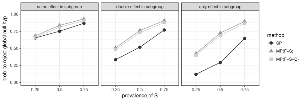
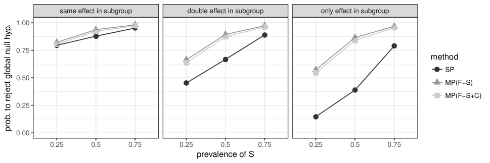
1.1 Results for other data-generating models

Method	global	F	S	C
SP	0.05	0.05	-	-
MP-Pooled(F+S)	0.05	0.03	0.03	-
MP-Pooled(F+S+C)	0.05	0.03	0.02	0.02
MP-MultDF(F+S)	0.05	0.03	0.02	-
MP-MultDF(F+S+C)	0.05	0.02	0.02	0.02

Table 6: Probability to reject the global null hypothesis and population null hypotheses for single population (SP) and multi-population (MP) testing methods. Data are generated from a constant model under homoscedasticity.

		Scenario and Prevalence
		same	same	same	double	double	double	only	only	only
Method	Population	0.25	0.5	0.75	0.25	0.5	0.75	0.25	0.5	0.75
SP	global	0.88	0.88	0.87	0.54	0.67	0.79	0.16	0.40	0.66
MP-Pooled(F+S)	global	0.82	0.84	0.85	0.54	0.69	0.80	0.33	0.59	0.75
	F	0.81	0.82	0.83	0.43	0.58	0.73	0.10	0.32	0.60
	S	0.30	0.55	0.72	0.31	0.54	0.73	0.29	0.54	0.72
MP-Pooled(F+S+C)	global	0.82	0.82	0.82	0.51	0.64	0.75	0.30	0.52	0.69
	F	0.78	0.78	0.78	0.39	0.52	0.67	0.09	0.26	0.52
	S	0.27	0.49	0.65	0.28	0.48	0.66	0.26	0.48	0.65
	C	0.65	0.46	0.26	0.20	0.14	0.09	0.02	0.02	0.02
MP-MultDF(F+S)	global	0.83	0.85	0.87	0.53	0.69	0.81	0.35	0.58	0.75
	F	0.81	0.83	0.85	0.43	0.59	0.74	0.11	0.31	0.59
	S	0.28	0.55	0.74	0.29	0.55	0.72	0.31	0.54	0.72
MP-MultDF(F+S+C)	global	0.83	0.83	0.83	0.50	0.65	0.75	0.31	0.52	0.68
	F	0.78	0.79	0.79	0.39	0.53	0.67	0.09	0.26	0.51
	S	0.25	0.49	0.66	0.26	0.49	0.65	0.27	0.48	0.65
	C	0.66	0.48	0.26	0.20	0.13	0.09	0.02	0.02	0.02

Table 7: Probability to reject the global null hypothesis and population null hypotheses for single population (SP) and multi-population (MP) testing methods. Data are generated from a linear model under homoscedasticity.

		Scenario and Prevalence
		same	same	same	double	double	double	only	only	only
Method	Population	0.25	0.5	0.75	0.25	0.5	0.75	0.25	0.5	0.75
SP	global	0.86	0.86	0.86	0.51	0.65	0.76	0.16	0.36	0.64
MP-Pooled(F+S)	global	0.80	0.82	0.84	0.50	0.66	0.78	0.31	0.55	0.73
	F	0.78	0.80	0.82	0.41	0.56	0.70	0.10	0.29	0.58
	S	0.26	0.52	0.70	0.28	0.51	0.70	0.27	0.51	0.69
MP-Pooled(F+S+C)	global	0.80	0.80	0.80	0.47	0.61	0.72	0.28	0.49	0.67
	F	0.75	0.75	0.76	0.37	0.50	0.63	0.08	0.24	0.49
	S	0.23	0.45	0.63	0.24	0.44	0.63	0.24	0.45	0.63
	C	0.62	0.43	0.23	0.18	0.14	0.09	0.02	0.02	0.02
MP-MultDF(F+S)	global	0.81	0.82	0.85	0.49	0.66	0.79	0.30	0.55	0.74
	F	0.80	0.80	0.83	0.40	0.56	0.71	0.10	0.28	0.58
	S	0.27	0.52	0.71	0.26	0.50	0.71	0.26	0.51	0.71
MP-MultDF(F+S+C)	global	0.81	0.81	0.81	0.46	0.61	0.72	0.26	0.49	0.67
	F	0.76	0.76	0.77	0.36	0.50	0.64	0.08	0.23	0.49
	S	0.24	0.46	0.64	0.23	0.44	0.63	0.22	0.45	0.63
	C	0.62	0.44	0.24	0.18	0.13	0.09	0.02	0.02	0.02

Table 8: Probability to reject the global null hypothesis and population null hypotheses for single population (SP) and multi-population (MP) testing methods. Data are generated from an exponential model under homoscedasticity.

		Scenario and Prevalence
		same	same	same	double	double	double	only	only	only
Method	Population	0.25	0.5	0.75	0.25	0.5	0.75	0.25	0.5	0.75
SP	global	0.95	0.95	0.95	0.64	0.80	0.88	0.20	0.49	0.78
MP-Pooled(F+S)	global	0.92	0.93	0.94	0.64	0.81	0.90	0.42	0.70	0.87
	F	0.92	0.92	0.93	0.54	0.72	0.84	0.13	0.41	0.73
	S	0.38	0.66	0.85	0.39	0.67	0.85	0.38	0.67	0.85
MP-Pooled(F+S+C)	global	0.92	0.92	0.92	0.61	0.77	0.86	0.38	0.65	0.82
	F	0.90	0.90	0.90	0.50	0.67	0.80	0.11	0.36	0.66
	S	0.34	0.60	0.80	0.35	0.61	0.80	0.34	0.61	0.79
	C	0.80	0.60	0.35	0.27	0.19	0.11	0.02	0.02	0.02
MP-MultDF(F+S)	global	0.92	0.93	0.94	0.63	0.81	0.90	0.41	0.72	0.86
	F	0.92	0.92	0.93	0.53	0.72	0.85	0.13	0.41	0.73
	S	0.39	0.68	0.84	0.37	0.67	0.84	0.37	0.68	0.84
MP-MultDF(F+S+C)	global	0.92	0.92	0.92	0.60	0.76	0.86	0.37	0.66	0.81
	F	0.90	0.90	0.90	0.49	0.66	0.80	0.11	0.35	0.66
	S	0.34	0.62	0.78	0.32	0.61	0.79	0.33	0.62	0.79
	C	0.80	0.60	0.34	0.25	0.20	0.11	0.02	0.02	0.02

Table 9: Probability to reject the global null hypothesis and population null hypotheses for single population (SP) and multi-population (MP) testing methods. Data are generated from a logistic model under homoscedasticity.

		Scenario and Prevalence
		same	same	same	double	double	double	only	only	only
Method	Population	0.25	0.5	0.75	0.25	0.5	0.75	0.25	0.5	0.75
SP	global	0.79	0.80	0.79	0.43	0.57	0.68	0.14	0.31	0.54
MP-Pooled(F+S)	global	0.73	0.75	0.77	0.42	0.58	0.70	0.26	0.47	0.65
	F	0.71	0.72	0.74	0.33	0.48	0.62	0.08	0.24	0.48
	S	0.22	0.42	0.61	0.23	0.43	0.62	0.23	0.43	0.61
MP-Pooled(F+S+C)	global	0.72	0.71	0.72	0.39	0.53	0.64	0.24	0.41	0.57
	F	0.67	0.66	0.67	0.29	0.42	0.54	0.07	0.20	0.40
	S	0.19	0.37	0.53	0.20	0.37	0.54	0.20	0.37	0.54
	C	0.53	0.36	0.21	0.15	0.11	0.07	0.02	0.02	0.02
MP-MultDF(F+S)	global	0.72	0.74	0.78	0.42	0.58	0.69	0.25	0.47	0.65
	F	0.70	0.72	0.74	0.33	0.48	0.61	0.08	0.24	0.49
	S	0.23	0.42	0.62	0.23	0.44	0.60	0.22	0.43	0.61
MP-MultDF(F+S+C)	global	0.72	0.72	0.73	0.40	0.53	0.62	0.23	0.41	0.58
	F	0.66	0.67	0.67	0.29	0.42	0.53	0.07	0.20	0.40
	S	0.20	0.36	0.54	0.19	0.38	0.52	0.19	0.37	0.54
	C	0.52	0.36	0.20	0.14	0.11	0.07	0.02	0.02	0.03

Table 10: Probability to reject the global null hypothesis and population null hypotheses for single population (SP) and multi-population (MP) testing methods. Data are generated from a quadratic model under homoscedasticity.

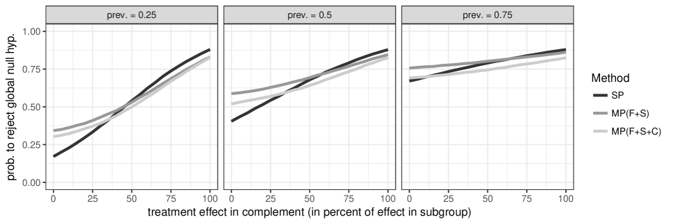
1.2 Detailed power curves

Figure 5: Probability to reject the global null hypothesis for single population (SP) and multi-population (MP) testing methods plotted against the treatment effect in the complement in relation to the subgroup. Data are generated from an Emax model under homoscedasticity.

Figure 6: Probability to reject the global null hypothesis for single population (SP) and multi-population (MP) testing methods plotted against the treatment effect in the complement in relation to the subgroup. Data are generated from a linear model under homoscedasticity.

Figure 7: Probability to reject the global null hypothesis for single population (SP) and multi-population (MP) testing methods plotted against the treatment effect in the complement in relation to the subgroup. Data are generated from an exponential model under homoscedasticity.

Figure 8: Probability to reject the global null hypothesis for single population (SP) and multi-population (MP) testing methods plotted against the treatment effect in the complement in relation to the subgroup. Data are generated from a logistic model under homoscedasticity.

Figure 9: Probability to reject the global null hypothesis for single population (SP) and multi-population (MP) testing methods plotted against the treatment effect in the complement in relation to the subgroup. Data are generated from a quadratic model under homoscedasticity.

2 Additional simulation results for heteroscedastic scenarios

2.1 Comparison of approximate tests for other data-generating models

Figure 10: Probability to reject the global null hypothesis for single population (SP) and multi-population (MP) testing methods. Data are generated from a linear model under heteroscedasticity. MP-MultDF is used to approximate the joint distribution for MP testing methods.

Figure 11: Probability to reject the global null hypothesis for single population (SP) and multi-population (MP) testing methods. Data are generated from an exponential model under heteroscedasticity. MP-MultDF is used to approximate the joint distribution for MP testing methods.

Figure 12: Probability to reject the global null hypothesis for single population (SP) and multi-population (MP) testing methods. Data are generated from a logistic model under heteroscedasticity. MP-MultDF is used to approximate the joint distribution for MP testing methods.

Figure 13: Probability to reject the global null hypothesis for single population (SP) and multi-population (MP) testing methods. Data are generated from a quadratic model under heteroscedasticity. MP-MultDF is used to approximate the joint distribution for MP testing methods.

2.2 Comparison of multi-population MCP to single population MCP for other data-generating models

Figure 14: Probability to reject the global null hypothesis for single population (SP) and multi-population (MP) testing methods. Data are generated from a linear model under heteroscedasticity. MP-MultDF is used to approximate the joint distribution for MP testing methods.

Figure 15: Probability to reject the global null hypothesis for single population (SP) and multi-population (MP) testing methods. Data are generated from an exponential model under heteroscedasticity. MP-MultDF is used to approximate the joint distribution for MP testing methods.

Figure 16: Probability to reject the global null hypothesis for single population (SP) and multi-population (MP) testing methods. Data are generated from a logistic model under heteroscedasticity. MP-MultDF is used to approximate the joint distribution for MP testing methods.

Figure 17: Probability to reject the global null hypothesis for single population (SP) and multi-population (MP) testing methods. Data are generated from a quadratic model under heteroscedasticity. MP-MultDF is used to approximate the joint distribution for MP testing methods.

References

- [1] Foster JC, Taylor JM, Ruberg SJ. Subgroup identification from randomized clinical trial data. Statistics in Medicine 2011; 30(24):2867–2880.
- [2] Lipkovich I, Dmitrienko A, Denne J, Enas G. Subgroup identification based on differential effect search—a recursive partitioning method for establishing response to treatment in patient subpopulations. Statistics in Medicine 2011; 30(21):2601–2621.
- [3] Seibold H, Zeileis A, Hothorn T. Model-based recursive partitioning for subgroup analyses. International Journal of Biostatistics 2016; 12(1):45–63, doi:10.1515/ijb-2015-0032.
- [4] Varadhan R, Wang SJ. Treatment effect heterogeneity for univariate subgroups in clinical trials: Shrinkage, standardization, or else. Biometrical Journal 2016; 58:133–153.
- [5] Rosenkranz G. Exploratory subgroup analysis in clinical trials by model selection. Biometrical Journal 2016; 58:1217–1228.
- [6] Shen C, Hu Y, Li X, Wang Y, Chen PS, Buxton AE. Identification of subpopulations with distinct treatment benefit rate using the Bayesian tree. Biometrical Journal 2016; 58(6):1357–1375.
- [7] Liu J, Sivaganesan S, Laud PW, Müller P. A Bayesian subgroup analysis using collections of anova models. Biometrical Journal 2017; 59(4):746–766.
- [8] Lipkovich I, Dmitrienko A, D’Agostini RB. Tutorial in biostatistics: data-driven subgroup identification and analysis in clinical trials. Statistics in Medicine 2017; 36(1):136–196, doi:10.1002/sim.7064.
- [9] Koch GG. Discussion of p-value adjustments for subgroup analyses. Journal of Biopharmaceutical Statistics 1997; 7(2):323–331.
- [10] Alosh M, Huque MF. A flexible strategy for testing subgroups and overall population. Statistics in Medicine 2009; 28(1):3–23.
- [11] Ondra T, Dmitrienko A, Friede T, Graf A, Miller F, Stallard N, Posch M. Methods for identification and confirmation of targeted subgroups in clinical trials: a systematic review. Journal of Biopharmaceutical Statistics 2016; 26(1):99–119.
- [12] Bretz F, Maurer W, Brannath W, Posch M. A graphical approach to sequentially rejective multiple test procedures. Statistics in Medicine 2009; 28(4):586–604.
- [13] Bretz F, Posch M, Glimm E, Klinglmueller F, Maurer W, Rohmeyer K. Graphical approaches for multiple comparison procedures using weighted bonferroni, simes, or parametric tests. Biometrical Journal 2011; 53(6):894–913.
- [14] Thomas M, Bornkamp B, Seibold H. Subgroup identification in dose-finding trials via model-based recursive partitioning. Statistics in Medicine 2018; .
- [15] Bretz F, Pinheiro JC, Branson M. Combining multiple comparisons and modeling techniques in dose-response studies. Biometrics 2005; 61(3):738–748.
- [16] Pinheiro J, Bornkamp B, Glimm E, Bretz F. Model-based dose finding under model uncertainty using general parametric models. Statistics in Medicine 2014; 33(10):1646–1661.
- [17] Pinheiro J, Bornkamp B, Bretz F. Design and analysis of dose-finding studies combining multiple comparisons and modeling procedures. Journal of Biopharmaceutical Statistics 2006; 16(5):639–656.
- [18] Xun X, Bretz F. The MCP-Mod methodology: Practical considerations and the DoseFinding R package. Handbook of Methods for Designing, Monitoring, and Analyzing Dose-finding Trials, O’Quigley J, Iasonos A, Bornkamp B (eds.). chap. 12, CRC Press, 2017.
- [19] Hasler M. Multiple contrast tests for multiple endpoints in the presence of heteroscedasticity. The International Journal of Biostatistics 2014; 10(1):17–28.
- [20] Graf AC, Wassmer G, Friede T, Gera RG, Posch M. Robustness of testing procedures for confirmatory subpopulation analyses based on a continuous biomarker. submitted for publication 2018; .
- [21] Millen BA, Dmitrienko A, Ruberg S, Shen L. A statistical framework for decision making in confirmatory multipopulation tailoring clinical trials. Drug Information Journal 2012; 46(6):647–656.
- [22] Bretz F, König F, Bornkamp B. Multiple test strategies for comparing several doses with a control in confirmatory trials. Handbook of Methods for Designing, Monitoring, and Analyzing Dose-finding Trials, O’Quigley J, Iasonos A, Bornkamp B (eds.). chap. 16, CRC Press, 2017.
- [23] Bornkamp B, Ohlssen D, Magnusson BP, Schmidli H. Model averaging for treatment effect estimation in subgroups. Pharmaceutical Statistics 2017; 16(2):133–142.