Spatio-Temporal Road Scene Reconstruction Using Superpixel Markov Random Field
Abstract
Scene model construction based on image rendering is an indispensable but challenging technique in computer vision and intelligent transportation systems. In this paper, we propose a framework for constructing 3D corridor-based road scene models. This consists of two successive stages: road detection and scene construction. The road detection is realized by a new superpixel Markov random field (MRF) algorithm. The data fidelity term in the MRF’s energy function is jointly computed according to the superpixel features of color, texture and location. The smoothness term is established on the basis of the interaction of spatio-temporally adjacent superpixels. In the subsequent scene construction, the foreground and background regions are modeled independently. Experiments for road detection demonstrate the proposed method outperforms the state-of-the-art in both accuracy and speed. The scene construction experiments confirm that the proposed scene models show better correctness ratios, and have the potential to support a range of applications.
keywords:
Superpixel , Markov random field , region detection , scene modeling1 Introduction
With the rapid development of information science and computer vision, scene construction based on image rendering has become an important feature of many applications. Scene construction results are of particular use when seeking to simulate real-world events. There are three kinds of applications typically associated with scene construction: (1) Virtual street views [3, 29]. Road image sequences contain lots of information people may find useful. In response to this, Google sent out a fleet of cars to capture road images from all over the world. The Google Street View system was developed to allow users to tour street scenes while browsing a map. Another similar application is Microsoft Street Slide, which introduces scene bubbles that users can interact with. (2) Intelligent transportation systems [21, 30]. Advanced driver assistant systems (ADAS) are be improved through virtual scene reconstruction. In contrast to traditional field tests of unmanned vehicles, an evaluation can be implemented in a virtual environment. The simulation-based evaluation system can handle thousands of quantitative judgments in a short time and be more objective than a human expert [31]. (3) Free viewpoint television [33, 45]. Virtual reality technology is commonly used in the modern film industry. Free viewpoint video has become popular because, it provides users with richer interactions. Users can freely select their viewpoint while browsing videos by drawing upon free viewpoint rendering methods.
In early studies, virtual scenes were constructed by using computer graphics approaches. Typical examples include the Prescan software 111http://www.tassinternational.com/prescan, and IPG Co.’s CarMaker software [22]. Alongside of computer graphics methods, road scene construction from image sequences became popular. The Waymo team at Google proposed a virtual platform for scene modeling from road images, utilizing machine learning methods, with off-line testing of unmanned vehicles being conducted using the platform. Recently, generative adversarial networks (GAN) have been proposed that can synthesize virtual traffic scenes [18]. However, all of these methods have a variety of limitations, including issues with modeling both the foreground and background, rendering of new viewpoint images, and so on.
Traditional reconstruction of road scene methods do not distinguish between the foreground and background regions, such as the framework of Google Street View [3] and Microsoft Street Slide [29]. Tour into the picture (TIP) framework models both the foreground and background regions of an image [24, 25, 32]. After the specification of the vanishing point, the background model is roughly composed of “left wall”, “right wall”, “back wall”, “sky” and “road plane”. The foreground models can be constructed independently of the background models. However, the TIP model is not fit for the curved-edge road conditions. In this paper, a new framework to model 3D scenes is introduced using David Marr’s theory [36], which builds upon the vision framework of “feature map computation-depth recovery-3D modeling”. The idea of the TIP model is also incorporated, which implements the region detection and semantic reasoning to automatically construct the 3D road scenes. The road regions of an input image sequence are detected via a new superpixel-based Markov random field (MRF) method, with each superpixel refering to a group of connected pixels of a similar color. An energy function is defined that is based on vision features computed in the spatio-temporal domain. An energy minimization process is conducted following a cycle of “global energy initialization-local energy comparison-global energy comparison”. After the detection of road regions, 3D corridor-structured scene models are constructed, based on road boundary control points. The road regions are assumed to be on a horizontal plane, while the rest of the scene components are treated as standing perpendicularly to the road plane. Panoramic scene models can also be constructed, and it can serve as the basis for a range of potential applications, such as virtual street view, traffic scene simulations, etc.
The main contributions of this paper are threefold:
-
1.
A new superpixel-based MRF method that can detect road regions in image sequences. The data fidelity term in the MRF’s energy function is defined according to a combination of superpixel features of color, texture and location. Its smoothness term is computed according to the feature distance between of spatio-temporally adjacent superpixels. Energy minimization is implemented by means of a “global energy initialization-local energy comparison-global energy comparison” cycle.
-
2.
A novel framework to construct road scene models automatically from image sequences. The road scene model has a 3D corridor structure, with the road regions being assumed to be horizontal planes. Foreground objects are modeled independently of the background models. Panoramic scene models can also be constructed.
-
3.
A new intelligent system for interactive tour in traffic scenes, based on the proposed scene models. Two basic modes are designed: bird’s eye view mode; and touring mode. New traffic elements can be inserted into the traffic scenes, which can be used for virtual simulations with unmanned vehicles.
2 Related Works
The research presented in this paper focuses on road detection via superpixel-based MRF, and on scene model reconstruction. Below, we discuss the related research for each of these components, respectively:
(1) Region detection: The semantic analysis of road images is an important part of 3D road scene reconstruction. Road detection underpins this semantic analysis. Belaid et al. have proposed a watershed transformation method, that can be applied to road region detection [5]. A topological gradient method is used to avoid over segmentation. Chen et al. [11] proposed a mechanism to support the long-term background and short-term foreground models. A unified Bayesian framework is utilized in the background-foreground fusion stage. Song et al. [43] have propose a new method for image appearance transfer that combines color and texture features. To do this, they imlemented feature detection and matching between source and reference images. The image and geometric features were then able to be exploited. Xiao et al. [48] have sought to extend the traditional conditional random field (CRF) model by proposing a hybrid CRF model that integrates the camera information and LIDAR. The hybrid CRF model can be optimized with graph cuts to acquire road regions. However, there is a dependency upon LIDAR information for this approach to work. Kim et al. [27] have introduced a search method based on a coarse-to-fine strategy and image superpixels. A simple generative appearance model is applied during the initial coarse step. In the refine step, a sampling and similarity measurement process is performed. Gould et al. [19] have presented a semantic segmentation method that uses label transfer. An approximate nearest neighbor algorithm is applied to build a graph upon the superpixels. Although this approach is effective for standard datasets, experiments using road image sequences have not always been satisfactory. Lu et al. [35] used an unsupervised method to select superpixel neighbors according to the GrowCut framework. However, for this to work the vanishing points have to be detected first, as a supplementary step.
(2) Superpixel-based MRF: Pixel-level MRF algorithms are widely used for image segmentation and annotation. Kim et al. [28] have applied an MRF model to image segmentation, that is especially effective for outdoor images. Yang et al. [50] have proposed a pixon-based MRF method for image segmentation. The basic idea of a “pixon” is that the spatial scale at each image site will vary according to the image information. However, the generation of pixons requires the solving of an anisotropic diffusion equation. Elia et al. [15] have proposed a tree-structured MRF model, that can be applied to Bayesian image segmentation. Here, the input image can be iteratively segmented into smaller regions based on a series of “split-merge” steps. However, pixel-based MRF methods are very susceptible to noise. Schick et al. [40] have proposed a superpixel-based MRF algorithm, that uses a classical Graphcut approach to energy minimization. The graph cut approach aims to solve the segmentation problem using max flow and min cut theory. However, the data fidelity term in the energy function is too simple to be able to reflect the irregular attributes of superpixels. Fulkerson et al. [17] have constructed a classifier by aggregating histograms of superpixel neighborhoods. A superpixel is a group of connected pixels with similar color information, which is a polygonal part of an image. The superpixel graph is then optimized by a CRF mechanism. However, superpixel features are insufficient in this method, and the spatio-temporal superpixel relationships are ignored. A variety of methods is proposed in [46], but these also have drawbacks relating to the insufficient use of temporal information, complex iterations of the energy function and low efficiency in the data fidelity terms. To overcome the drawbacks and limitations mentioned above, we are proposing here a new superpixel-based MRF algorithm that can detect road regions in images and videos. In our method, the date fidelity term of the energy function is combined with various types of superpixel features. The smoothness terms are computed according to the spatio-temporal proximity of superpixels.
(3) Scene model construction: 3D modeling and reconstruction is currently a hot topic in computer vision and computer graphics communities. With regard to the reconstruction of single objects, a number of important achievements have now been realized in relation to 3D building reconstruction, 3D model retrieval, 3D face simulation, etc. The general aim with all of these technologies is to recover the 3D geometric surface of single objects. As soon as one moves beyond single object reconstruction, 3D reconstruction becomes much more challenging. Saxena et al. [39] have put forward a plane parameters learning approach that is based on MRF. This is used to judge the location and orientation of recovered mesh facets. Make3D models with wireframe meshes are then constructed. The monocular image features used in this approach principally include color, texture, gradient and edges. The plane and model correctness ratios are utilized as metrics to evaluate the scene models. However, the method does not take into account the possible impact of large-scale semantic environments. Hoiem et al. [23] have developed an approach that first performs superpixel segmentation of input images, then applies support vector machine (SVM) to cluster superpixels with a similar appearance into cliques. The regional properties of the superpixel cliques are then specified to construct “pop up” style 3D scene models. Lou et al. [34] were the first to use layout templates to predict a global image structure. A random walk algorithm is then used to infer refined scene structures. However, the limited number of scene stages prevents this from being applied to all road scene structures.
The rest of the paper is organized as follows: In Section 3, an MRF model at pixel level is introduced. Our approach to region detection using superpixel-based MRF is described in Section 4. Section 5 details the spatio-temporal scene reconstruction process. The results of an experimental validation of the proposed framework are presented and discussed in Section 6. Section 7 provides our conclusions and indicates our future works.
3 MRF Model at Pixel Level
We are first of all going to introduce the pixel-level MRF model and how it works. Two groups of random variables, and , are defined. These refer to the observational data and state variables, respectively. The posterior probability distribution, , can be solved by using Bayesian theory [44]. For the task of image annotation, denotes the pixel coordinate set in the image, while denotes the corresponding set of labels. The constraint between these variables is established to compute , which is assumed to follow a uniform distribution. Assuming the elements in and are independent of each other, the likelihood function can be defined as follows:
| (1) |
where is the data fidelity term of the element.
Based on the above analysis, Eq.(2) can be defined by:
| (2) |
where denotes the uniform Gibbs distribution. The labels of and can be transformed to each other in the Gibbs distribution, as shown in Fig. 1. The function of makes the product of (pixels of label ) and (pixels of label ) to reach the maximum.
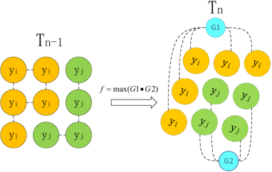
When the constant component is removed, the energy function is defined as follows:
| (3) |
The variable is solved by the minimization of energy function:
| (4) |
Several classic algorithms can be used for energy minimization, such as greedy algorithms and dynamic programming algorithms. A pixel-level MRF is useful for the image segmentation tasks, saliency detection, etc. However, pixels that are captured by a camera sensor are not meaningful units by themselves. They are also very susceptible to noise [40]. In order to improve their representational efficiency, we decided to use a new MRF model based on superpixels. The main merit of superpixels is that they provide a more natural and perceptually meaningful representation of an input image [41]. A superpixel representation greatly reduces the number of image primitives and is more robust to noise. Computation of a region’s visual features by superpixels is also more effective.
4 Spatio-temporal road region detection
Having established the pixel-level MRF model, we will now present the new superpixel-based MRF model, beginning with superpixel segmentation and feature pool construction.
4.1 Superpixels and Feature Pools
Thousands of superpixels may exist in a single still image. These are taken as mid-level image units. Useful image features can be generated by clustering the superpixels into cliques. Ideally, a superpixel clique will occupy an image region that represents a certain semantic object. However, the clique may not correspond to a semantic object even if all the superpixels have the same label. Superpixel features are widely used to assist with the tasks of image segmentation, semantic annotation, etc. These features primarily include color, texture and geometric shape, as shown in Table 1.
| Feature Descriptors | Feature Numbers |
|---|---|
| Color | 9 |
| C1 RGB color | 3 |
| C2 HSV color | 3 |
| C3 CIELAB | 3 |
| Texture | 62 |
| T1 Gabor filters: 4 scales, 6 orientations | 48 |
| T2 Local binary pattern: template | 9 |
| T3 Edge histogram descriptors | 5 |
| Locations and Shapes | 6 |
| L1 Location: Normalized and coordinates | 2 |
| L2 Shapes: Superpixel number in the clique | 1 |
| L3 Shapes: Edge number within convex hull | 1 |
| L4 Shapes: Ratio of the pixels to the convex hull | 1 |
| L5 Shapes: Whether the clique is continuous | 1 |
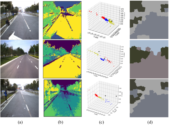
Color feature pools can be constructed using a self-organizing map (SOM) based on competitive learning [26]. The main advantage of using an SOM method rather than K-means clustering is the adaptive clustering it provides. Color feature clustering based on SOM involves three processes, competition, cooperation and adaptation, in which the Euclidean distance between input and output data is utilized. The mean and standard error for each superpixel belonging to a certain image region are computed in the CIELab space. The input is the superpixel color information within road regions in a set of training images. After specification of the neurons in the SOM network, the clustering means are computed without preassigning the clustering mean number. The SOM clustering results are assumed to be the color means in the feature pool. Fig. 2 shows examples of color feature clustering using SOM.
To represent the texture features, the local texture is represented by the intensity distribution of adjacent pixels. The global texture is defined by assembling the local texture information. The texture feature pools are constructed by clustering the Gabor filter outputs for all of the image regions [4]. For each pixel in the image, a corresponding Gabor filter output vector is computed. We chose to implement a Gabor filter with 4 scales and 6 directions. So, the output vector dimension for a sized Gabor filter is . The computation for such high-dimensional feature vector is very time-consuming. Besides, serious feature redundance can be suffered. So, we only chose to concentrate on just the mean and the standard error of the Gabor filter output. As a result, there is only feature dimension to be concerned with.
4.2 Road Region Detection
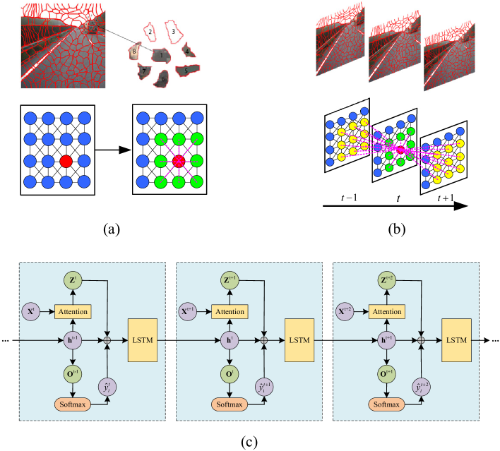
After constructing the feature pools, we introduce a road region detection algorithm that utilized the superpixel-based MRF. The connections between spatially and spatio-temporally adjacent superpixels are shown in Fig. 3 (a) and (b). The red dots in the figure denote the current superpixel for processing. The green dots denote the spatially adjacent superpixels. The yellow dots relate to adjacent superpixels in both spatial and temporal domains.
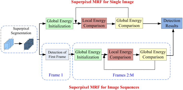
Fig. 4 shows the flow diagram of the road detection process, which works for both single images and image sequences. We will focus here on the algorithm for image sequences. In this algorithm, the global energy for the superpixel-based MRF is as follows:
| (5) |
where denotes the superpixel set; is the appearance feature of the superpixel at time ; denotes the label of the superpixel, which is in the set of ; denotes the data fidelity term of the superpixel; is the smoothness term of the adjacent superpixel pairs; and denote the adjacent neighbors of superpixel in spatial and temporal domains, respectively; and are constants.
The probability of the data fidelity term is computed as follows, using a combination of color, texture and location information for any time :
| (6) |
where , and denote the color, texture and location features of the superpixel, respectively.
The color probability is defined by the following three-channel Gaussian distribution:
| (7) |
where and are the mean and covariance in the color feature pool corresponding to label .
The road region usually contains a rich variety of textural materials and stripes. The texture features can be used to compute the probability of the data fidelity term as an additional measure. We employ a Gabor filter to extract the texture features. The image block centered upon each superpixel is used to compute the output vectors of the Gabor filter. The computation is implemented by using a correlation coefficient together with the cluster means in the texture feature pool. The exponential form of the largest coefficient is defined as the texture probability:
| (8) |
where denotes the clustering mean in the texture feature pool ; and is the correlation coefficient:
| (9) |
where denotes the dimension of texture feature vector.
The location probability is computed as follows:
| (10) |
For the computation of the location probability, the input image is projected onto a rectangle. denotes the locations in the rectangle. For the training set, the same projection method is applied. denotes the number of superpixels belonging to the label , corresponding to the location in the regular rectangle. denotes the total number of superpixels in location of the regular rectangle. is set to be a certain small value, e.g. . The constant, , varies according to the different datasets.
After computation of the data fidelity term, the smoothness term can be defined as:
| (11) |
where denotes the distance between the superpixel feature vectors:
| (12) |
where and are the color features of and superpixels; is a positive semi-definite matrix that parameterizes the metric. The metric is Euclidean norm when . The metric is the Mahalanobis distance when , where denotes the inverse covariance matrix. is the Kronecker delta:
| (15) |
The constant coefficient, , can be defined as follows:
| (16) |
where denotes the expectation of the superpixel pairs.
In addition to the global energy function, the local energy function for the superpixel is as follows:
| (17) |
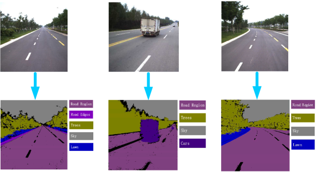
Working on the assumption that frames exist in the image sequence, the proposed superpixel-based MRF algorithm is shown in Algorithm 1. The label initialization for the first frame is implemented using a semantic labeling method [8], as shown in Fig. 5. The semantic labeling method incorporates three different image segmentation methods: GraphCut [16], MeanShift [12] and Image Pyramid method [10]. Although this semantic labeling method achieves a more accurate initialization, we only chose to apply it to initialize the first frame, because it requires too much human interaction and is very time-consuming.
For the rest of the frames, the superpixel initialization is implemented by a long short-term memory (LSTM) network, as shown in Fig. 3 (b). Beginning with the LSTM network training process, for the superpixel in the frame, the LSTM input data includes the superpixel feature vector , and the corresponding ground truth superpixel label , where ; denotes the superpixel number. The output of the LSTM network is compared with the ground truth superpixel label , and a cross entropy function is used to compute the error.
After this, the trained LSTM network is used for the initialization of the superpixel labels for each frame. The input to the LSTM is again for the superpixel in frame . and denote the hidden states of the LSTM network at time and , respectively. is the weighted feature based on the attention mechanism [49]. is the output of the LSTM network at time . and are the initialized labels for the superpixel at times and , respectively.
After the superpixel initialization step, the road detection algorithm is designed to follow a cycle of “initial energy computation-local energy comparison-global energy comparison”. The smoothness term of the energy function incorporates the superpixel interactions in both the spatial and temporal domains. We assume that the road region between adjacent frames has barely changed, and apply the superpixel centers from the previous frame to initialize the current one. An optical flow map is also used to match the superpixels in adjacent frames, in case the road region between adjacent frames has changed more significantly. The optical flow map is computed according to Bruhn’s method [9], which is applied to align the superpixel centers of the current frame with the nearest centers in adjacent frames.
Drawing upon the initial superpixel labels, the initial global energy function can be computed using Eq. (7). The value of is the sum of the local energy function . The energy function is composed of a data fidelity term and a smoothness term. The data fidelity term is defined by a combination of color, texture and location probabilities. The smoothness term is defined by the interaction between spatially adjacent superpixels (Eq. 13). After computation of the global energy function, the local energy of superpixel is calculated according to Eq. (8). An swap is then applied for the label , and the new local energy is compared to . If the new local energy has reduced, the current class label is displaced. The swap method has a similar mechanism as -expansion [7], which is widely used in energy minimization. After the comparison of all the local energies, the global energy is updated. If and the previous value of are within a small threshold distance , the algorithm terminates.
%ͨ µ ǰ ǩ 𣬼 µľֲ ̵ֵ ԭ оֲ ̵ֵ бȽϣ µľֲ ̵ֵ С ǰ ǩ 滻 ǰ ǩ
The proposed algorithm can be implemented for each single image independently.
Under such conditions, the smoothness term of the energy function only takes into account the spatially neighboring superpixels.
However, running the algorithm for complete image sequences of images offers certain advantages:
-
1.
Smoothness term. The smoothness term for image sequences incorporates the neighboring superpixels in both the spatial and temporal domains.
-
2.
Initialization of the labels for the first frame. The superpixel-based MRF method for image sequences applies more accurate semantic labeling to initialize the first frame.
-
3.
Initialization of the labels for the rest of the frames. In the superpixel-based MRF method for image sequences, the LSTM network is applied to initialize the superpixel labels for the rest of the frames.
5 Spatio-Temporal Scene Reconstruction
After detecting the road regions in the input image sequences, control points on the road boundaries are generated to represent the road geometry. Then, the road scene models are constructed based on the control points. Several steps are needed to generate these control points. Firstly, the vanishing point for each input image is detected by a Gaussian sphere method [6]. Secondly, the detected road regions are then processed for image binarization. After this, the road boundaries can be generated based on the road and non-road regions. Given the constraint of thevanishing points, the potential farthest control points can be identified. The points where the road boundaries intersect with the image edges are defined as the nearest control points. The other control points are assumed to be uniformly distributed between the nearest and farthest control points. A 3D corridor-style scene model can then be constructed based on the control points. We apply the Manhattan world assumption [13] to specify the world coordinate system. The scene models are assumed to follow a Cartesian coordinate system. Viewers can get interpretations of the road scene by changing the alignment of the system.
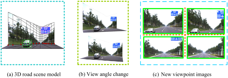
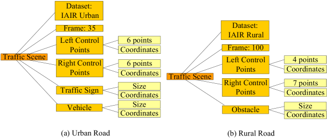
The background models for the 3D corridor structure can be constructed on the basis of the detection results for the road regions. The road region is set as a horizontal plane and, the rest of the background regions are assumed to stand perpendicularly to the road plane. If there are any foreground objects in the input image, a foreground/background segmentation method is adopted to construct the foreground and background models independently [11]. The foreground models are constructed with an data structure, where denotes the transparency ratio. The background inpainting is implemented by a process of “optical flow inpainting/image inpainting”. According to the 3D scene models, new viewpoint images can be generated by changing the views using OpenGL hardware texture mapping [32], as shown in Fig. 6. In order to properly structure the 3D corridor models, a scene model database is constructed. Each scene model corresponds to a frame in the image sequence, and a table to represent the connections between the foreground and background is defined [37], as shown in Fig. 7. The algorithm for road scene models construction is shown in Algorithm 2.
As well as the scene reconstruction for monocular images, panoramic images can be used for scene construction. The image stitching algorithm we used largely relates to global alignment and image blending [14]. In the global alignment stage, bundle adjustment, parallax removal and feature-based alignment are applied to roughly stitch together the input images. Out of a wide choice of possible projection models, a cylindrical projection model is especially effective. Other, de-ghosting and blending steps also need to be undertaken to create the output panoramas. After this, the panoramic scene models can be constructed.
6 Experiments and Applications
The platform used for our experiments was a computer with an Intel i5 processor @3.33GHZ and 16.0 GB RAM. The experiments for road region detection were implemented using MATLAB R14, while the scene construction experiments were based on the OpenGL Toolbox. For the road detection, we designed experiments using three datasets: the Bristol Dataset [20] ( pixel size, 500 frames); the Caltech Dataset [2] ( pixel size, 1000 frames); and the TSD-max Dataset 222http://trafficdata.xjtu.edu.cn/index.do ( pixel size, 2000 frames). The experiments for the scene model construction were mainly based on the TSD-max Dataset, which was constructed by the Institute of Artificial Intelligence and Robotics at Xi’an Jiaotong University. TSD-max is the basic dataset for the “Future Challenge”, a national annual competition for unmanned vehicles supported by the National Natural Science Foundation of China.
6.1 Road Detection Experiment
The proposed road detection method can be implemented for both single images (SMRF1) and image sequences (SMRF2). To quantitatively evaluate the road detection results, we apply the precision () and recall () metrics to compare them with ground truth road regions. Precision denotes the ratio of correct pixels to the detected road region, while recall denotes the ratio of the correct pixels to the benchmark road region. In our experiments, precision and recall are defined as follows:
| (18) |
where and denote the detected region and the ground truth, respectively. The score can be computed by combining and as follows:
| (19) |
The recall metric is emphasized if , while the precision is emphasized if .
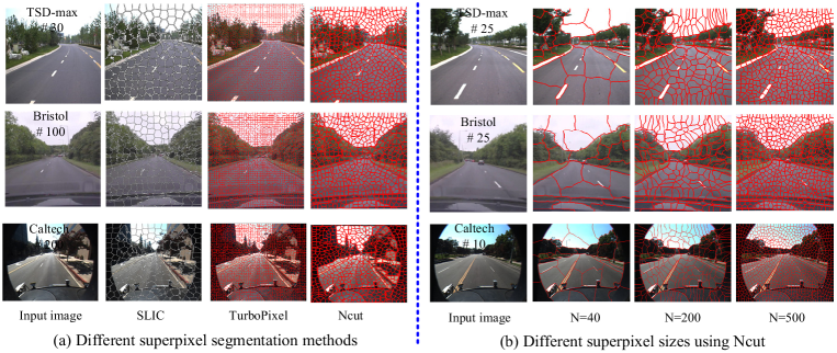
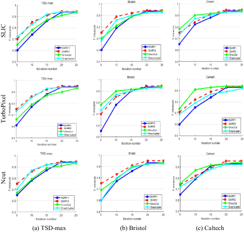
In the proposed method, superpixel segmentation is an important preliminary step. In Fig. 8 (a), three superpixel segmentation methods are compared: the SLIC method, which is based on K-means clustering [1]; the Turbopixel method, which is based on multidimensional eigen-images [47]; and the Ncut method, which is based on graph partitioning [42]. Superpixel segmentation can be implemented at different scales, as shown in Fig. 8 (b). Input images can be segmented using Ncut with the number of superpixels being set at , and . For the sake of feature selection and convergence speed, we choose for the experiments.
| GrowCut | GraphLabel | SMRF1 | SMRF2 | |
|---|---|---|---|---|
| TSD-max | 25 | 17 | 18 | 20 |
| Bristol | 24 | 17 | 20 | 20 |
| Caltech | 22 | 18 | 18 | 20 |
After specifying the number of superpixels, the influence of different numbers of iterations is evaluated. Comparisons are undertaken between the proposed methods SMRF1 and SMRF2, two state-of-the-art methods GrowCut [35] and GraphLabel [19], using the TSD-max, Bristol and Caltech datasets. The results based on different superpixel types are also compared. We compute the average () score for every 5 iterations, as depicted in Fig. 9. The comparison results indicate that, as the number of iterations increases, the score becomes more accurate. However, peak values are reached after 20 iterations for most of the datasets. Out of the three superpixel segmentation methods, Ncut obtains the most accurate results. The iteration speed of the proposed method is similar to the Graph label method, and ourperforms the GrowCut method. More detailed numbers of algorithm iterations are recorded in Table 2.
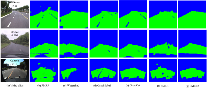
Furthermore, a comparison is made between the proposed methods (SMRF1 and SMRF2) and state of the art methods. The pixel-based MRF [15] is implemented based on a tree-structured MRF model, which segment the input image into smaller regions following a “split-merge” strategy. The Watershed method [5] uses a topological gradient approach to avoid over segmentation. The Graph label method [19] is based on label transfer and, uses an approximate nearest neighbor algorithm. In the GrowCut framework [35], the superpixel-level seeds are selected using an unsupervised way, and the superpixel neighbors are detected. The Superpixel-based conditional random field (SCRF) method [17] regularizes a classifier by aggregating histograms in the superpixel neighborhoods, and apply a conditional random filed model for refinement.
| Datasets | Methods | Precision | Recall | score | ||
|---|---|---|---|---|---|---|
| =0.5 | =1 | =2 | ||||
| TSD-max | PMRF [15] | 0.8625 | 0.8830 | 0.8665 | 0.8726 | 0.8788 |
| Watershed [5] | 0.8870 | 0.8920 | 0.8880 | 0.8895 | 0.8910 | |
| Graph label [19] | 0.9410 | 0.9425 | 0.9423 | 0.9442 | 0.9462 | |
| GrowCut [35] | 0.9310 | 0.9425 | 0.9333 | 0.9367 | 0.9402 | |
| SCRF [17] | 0.7680 | 0.7920 | 0.7727 | 0.7798 | 0.7871 | |
| SMRF1+S1 | 0.9320 | 0.9370 | 0.9330 | 0.9345 | 0.9360 | |
| SMRF1+S2 | 0.9380 | 0.9290 | 0.9362 | 0.9335 | 0.9308 | |
| SMRF1+S3 | 0.9385 | 0.9325 | 0.9373 | 0.9355 | 0.9337 | |
| SMRF2+S1 | 0.9465 | 0.9550 | 0.9482 | 0.9507 | 0.9533 | |
| SMRF2+S2 | 0.9410 | 0.9495 | 0.9427 | 0.9452 | 0.9478 | |
| SMRF2+S3 | 0.9405 | 0.9535 | 0.9431 | 0.9470 | 0.9509 | |
| Bristol | PMRF [15] | 0.8425 | 0.8320 | 0.8404 | 0.8372 | 0.8341 |
| Watershed [5] | 0.8375 | 0.8565 | 0.8412 | 0.8469 | 0.8526 | |
| Graph label [19] | 0.9250 | 0.9305 | 0.9261 | 0.9277 | 0.9294 | |
| GrowCut [35] | 0.9350 | 0.9410 | 0.9362 | 0.9380 | 0.9398 | |
| SCRF [17] | 0.8250 | 0.8275 | 0.8255 | 0.8262 | 0.8270 | |
| SMRF1+S1 | 0.9295 | 0.9340 | 0.9304 | 0.9317 | 0.9331 | |
| SMRF1+S2 | 0.9350 | 0.9400 | 0.9360 | 0.9375 | 0.9390 | |
| SMRF1+S3 | 0.9345 | 0.9315 | 0.9339 | 0.9330 | 0.9321 | |
| SMRF2+S1 | 0.9400 | 0.9485 | 0.9417 | 0.9442 | 0.9468 | |
| SMRF2+S2 | 0.9360 | 0.9580 | 0.9403 | 0.9469 | 0.9535 | |
| SMRF2+S3 | 0.9480 | 0.9552 | 0.9494 | 0.9516 | 0.9538 | |
| Caltech | PMRF [15] | 0.8210 | 0.7945 | 0.8156 | 0.8075 | 0.7997 |
| Watershed [5] | 0.6250 | 0.6500 | 0.6298 | 0.6373 | 0.6448 | |
| Graph label [19] | 0.9320 | 0.9200 | 0.9296 | 0.9260 | 0.9224 | |
| GrowCut [35] | 0.9500 | 0.9480 | 0.9496 | 0.9490 | 0.9484 | |
| SCRF [17] | 0.8185 | 0.8310 | 0.8210 | 0.8247 | 0.8285 | |
| SMRF1+S1 | 0.9290 | 0.9410 | 0.9314 | 0.9350 | 0.9385 | |
| SMRF1+S2 | 0.9220 | 0.9370 | 0.9250 | 0.9294 | 0.9340 | |
| SMRF1+S3 | 0.9325 | 0.9280 | 0.9316 | 0.9302 | 0.9289 | |
| SMRF2+S1 | 0.9420 | 0.9485 | 0.9433 | 0.9452 | 0.9472 | |
| SMRF2+S2 | 0.9380 | 0.9270 | 0.9350 | 0.9320 | 0.9290 | |
| SMRF2+S3 | 0.9560 | 0.9520 | 0.9552 | 0.9540 | 0.9528 | |
The detection results based on these state-of-the-art methods are depicted in Fig. 10, with green and blue denoting the detected road regions and the non-road regions, respectively. The results prove that the proposed method (SMRF2) achieves the most accurate detection results from the point-of-view of visual aesthetics. The other methods perform less well than our own, with the vehicle and road regions appearing too similar. The reason that PMRF and Watershed methods perform worse than the proposed methods is that they lack the statistical features of superpixels. The Graph label and GrowCut methods ignore the sptio-temporal interactions between adjacent superpixels.Aside from the qualitative comparisons, evaluations are undertaken on the basis of the score, as summarized in Table 3. The parameter is variously set to 0.5, 1 and 2. As mentioned above, the detection precision is emphasized when , while the recall is emphasized when . The state-of-the-art methods are again implemented for comparison. We compute the average score over all of the complete image sequences for each dataset. The comparative results show that the scores for SMRF2 are more than 0.927 for all 3 datasets, outperforming PMRF, Watershed, Graph label and Grow cut. This result is consistent with the qualitative results shown in Fig. 10. We also evaluate the results for different superpixel segmentations, with S1, S2 and S3 denoting the segmentations for TurboPixel [47], SLIC [1] and Ncut [42], respectively. The other methods are also implementedusing the different superpixel types, however, we only record their best performances. Comparison reveals that the proposed SMRF2 method outperformes all of the other methods. The results of SMRF1 are similar to the Graph label method. Among the three superpixel segmentation types, the highest are reached by the Ncut method.
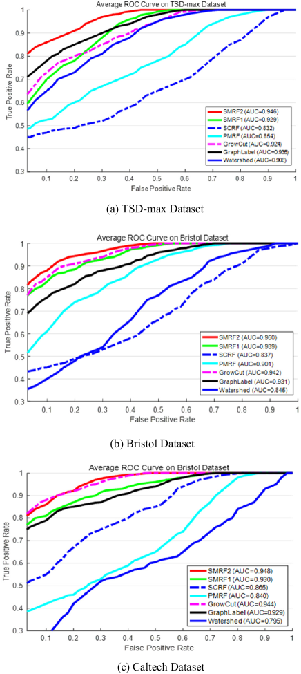
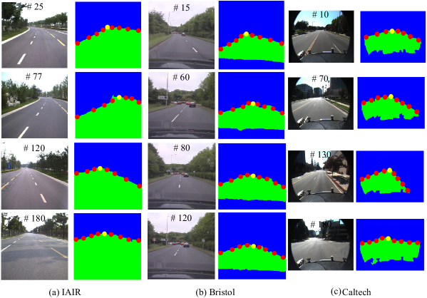
Moreover, we compare the average receiver operating characteristic (ROC) curves on the pixelwise comparison between the detected road regions and the ground truth. ROC curves denote the tradeoff between the true positive rate and the false positive rate . and are the number of road pixels correctly detected and the background pixels correctly deteccted, respectively. and are the number of background pixels incorrectly marked and the road pixels incorrectly identified, respectively. The area under curve (AUC) metric can be easily evaluated based on the ROC curves. As the comparison results show, the highest AUC value is provided by the proposed SMRF2 method for all the datasets; see Fig. 11. The performances of SMRF2 and GrowCut method are similar based on the Caltech dataset. The performances of the SMRF1 method are better than PMRF and Watershed methods. Further detection results for SMRF2 are depicted in Fig. 12, along with the control points and vanishing points.
6.2 Scene construction Experiment
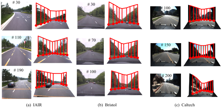
Based on the road detection results, we evaluate the accuracy and effectiveness of the road scene models. Scene models based on the different datasets are shown in Fig. 13. We used a confusion matrix as a metric to evaluate the accuracy of the scene model components in pixels, with LW, RW, BW and RP denoting “left wall”, “right wall”, “back wall” and “road plane”, as shown in Fig. 14. The ground truth for scene models are annotated in advance. The evaluation results indicate the correctness ratios of the proposed scene models are beyond 0.9 for these scene components.

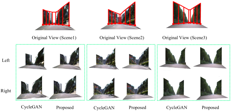
As we change the positions and angles of the scene models, new viewpoint images are generated by projecting the scene models onto the output image planes, as exhibited in Fig. 6. To assess the stability of the proposed scene models, we compare them to different view angles generated using CycleGAN [51]. The CycleGAN network consists of 2 generators and 2 discriminators. Images are generated based on the generators and discriminators at different view angles. Different view angle images are compared in Fig. 15. The results show that, compared to the proposed method, the textures of different view angle images using CycleGAN are fuzzy, and prone to distortion.
In order to quantitatively evaluate the proposed scene models, we apply two metrics [39]: (1) The plane correctness ratio, where a plane is defined as correct if more than 75% of its patches are correctly detected as semantic wall and road regions. (2) The model correctness ratio, where a model is defined as correct if more than 75% of its patches in the wall and road planes have a correct relationship to their neighbors. The ratio of plane patches to texture distortions is less than 25%.
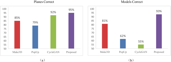
The evaluation was conducted by a person not associated with the project, who applied the above metrics. 1000 images from the TSD-max dataset are chosen for the experiment. Under these metrics, we compare the proposed models by Make3D [39], PopUp [23] and CycleGAN [51], as shown in Fig. 16. The results confirm that our models achieve both the best plane correctness ratio and the best model correctness ratio. The plane correctness ratio of CycleGAN method is close to us, however, its model correctness ratio is far inferior.
6.3 Applications
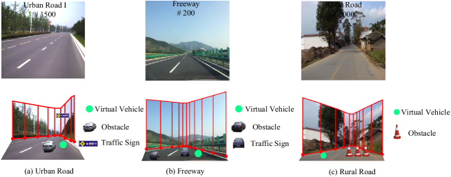
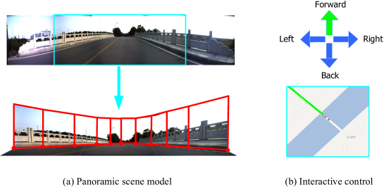
Various applications focused on traffic scene simulation can be developed based on the proposed scene models, as shown in Fig. 17. The composite system we propose here is named ‘Tour Into the Traffic Video’ (TITV). This can offer two simulation modes: (1) a bird’s-eye-view mode; and (2) a touring mode. In the bird’s-eye-view mode, the position, direction and speed of the virtual vehicle can be controlled by the user. Additional objects can be supplemented into the traffic scenes, such as obstacles, traffic signs, tower beacons, etc. Users can also observe the simulation from a bird’s-eye point-of-view. In the touring mode, new viewpoint images can be rendered as the viewpoint moves; see Fig. 4(b). The touring mode provides users with a feeling of actually being on the road.Panoramic scene models can also be constructed for the virtual street view, as shown in Fig. 18. Here, users can tour the street scenes using the commands “move forward”, “move back”, “turn left” and “turn right”, which are consistent with the actions of a real driver. At the same time, the tour trajectory is displayed on a map using GPS data.In Table 4, the functionalities of the proposed system are compared with those offered by Google Street View (GSV) [3] and Microsoft Street Slide (MSS) [29]. The results emphasize the novelty of our system, with it providing: (1) the scope to incorporate panoramas; (2) independent modeling of foreground objects; (3) generation of free viewpoint images; (4) display of map trajectories;
7 Conclusion and Future Works
In this paper, we have proposed a new framework for constructing spatio-temporal scene models from road image sequences. The reconstructed scene models have a 3D corridor structure, with road region detection being a precondition for scene construction. We have developed a new superpixel-based MRF method for road detection, which follows a cycle of “global energy initialization/local energy computation/global energy comparison”. The data fidelity term of the energy function is defined according to a combination of color, texture and location features. For both single images and image sequences, the smoothness term of the energy function is defined on the basis of superpixel interactions with spatially and spatio-temporally neighboring superpixels, respectively.On the basis of the road region detection results, road boundary control points are generated to construct the scene models. The scene models have a 3D corridor structure, with the road regions being assumed to be floor planes. Panoramic scene models can be constructed to offer users more choices. Applications for the simulation of unmanned vehicles have also been developed.In our future work, a depth map will be utilized as a supplement for scene reconstruction. On the basis of this, more detailed scene surface constructions can be implemented. We are also exploring ways to design algorithms that can detect additional label types, such as buildings and pedestrians.
Acknowledgment
This work is supported by National Natural Science Foundation of China under Grant No. 61803298, Natural Science Foundation of Jiangsu Province under Grant No. BK20180236, Suzhou Key Industry Technological Innovation (Perspective Application Research) under Grant No. SYG201843. The authors thank the anonymous reviewers for their valuable comments and suggestions.
References
- [1] R. Achanta, A. Shaji, K. Smith, et al., “SLIC superpixels compared to state-of-the-art superpixel methods,” IEEE Transactions on Pattern Analysis and Machine Intelligence, vol. 34, no. 11, pp. 2274-2282, 2012.
- [2] E. Aly, “Real time detection of lane markers in urban streets,” IEEE Intelligent Vehicles Symposium, pp. 7-12, 2008.
- [3] D. Anguelov, C. Dulong, D. Filip, et al., “Google street view: Capturing the world at street lebel,” Computer, vol. 42, no. 6, pp. 32-38, 2010.
- [4] J. Arrospide, L. Salgado, “Log-Gabor filters for image-based vehicle verification,” IEEE Transactions on Image Processing, vol. 22, no. 6, pp. 2286-2295, 2013.
- [5] L.J. Belaid, W. Mourou, “Image segmentation: A watershed transformation algorithm,” Image Analysis and Stereology, vol. 28, no. 1, pp. 93-102, 2009.
- [6] S.T. Bernard, “Interpreting perceptive images,” Artificial Intelligence, vol. 21, no. 1, pp. 453-462, 1983.
- [7] Y. Boykov, O. Veksler, and R. Zabih, “Fast approximate energy minimization via graph cuts,” IEEE Transactions on Pattern Analysis and Machine Intelligence, vol. 23, no. 11, pp. 1222-1239, 2001.
- [8] G.J. Brostow, J. Fauqueur, R. Cipolla, “Semantic object classes in video: A high-definition ground truth database,” Pattern Recognition Letters, vol. 30, no. 2, pp. 88-97, 2009.
- [9] A. Bruhn, J. Weickert, C. Schn, “Lucas/Kanade meets Horn/Shunk: Combining local and global optical flow methods,” International Journal of Computer Vision vol. 61, no. 3, pp. 211-231, 2005.
- [10] P. Burt, T. Hong, and A. Rosenfield, “Segmentation and estimation of image region properties through cooperative hierarchical computation,” IEEE Systems, Man and Cybernetics, vol. 11. no. 12, pp. 802-809, 1981.
- [11] Z. Chen, R. Wang, Z. Zhang, et al., “Background-foreground interaction for moving object detection in dynamic scenes,” Information Sciences, vol. 483, no. 1, pp. 65-81, 2019.
- [12] D. Comaniciu, P. Meer, “Mean shift: A robust approach toward feature space analysis,” IEEE Transactions on Pattern Analysis and Machine Intelligence, vol. 24, no. 5, pp. 603-619, 2002.
- [13] J.M. Coughlan, A.L. Yuille, “Manhattan world: Orientation and outlier detection by Bayesian interface,” Neural Computing, vol. 15, no. 5, pp. 1063-1088, 2003.
- [14] A. Eden, M. Uyttendaele, and R. Szeliski, “Seamless image stitching of scenes with large motions and exposure differences,” IEEE Conference on Computer Vision and Pattern Recognition, pp. 2498-2502, 2006.
- [15] C.D. Elia, G. Poggi, and G. Scarpa, “A tree-structured Markov random field model for Bayesian image segmentation,” IEEE Transactions on Image Processing, vo. 12, no. 10, pp. 1259-1273, 2003.
- [16] P. Felzenszwalb, D. Huttenlocher, “Efficient graph-based image segmentation,” International Journal of Computer Vision, vol. 59, no. 2, pp. 167-181, 2004.
- [17] B. Fulkerson, A. Vedaldi, and S. Soatto, “Class segmentation and object localization with superpixel neighborhoods,” IEEE International Conference on Computer Vision, pp. 670-677, 2009.
- [18] Y. Ganin, E. Ustinova, H. Ajakan, et al., “Domain adversarial training of neural networks,” Journal of Machine Learning Research, vol. 17, no. 59, pp. 1-35, 2016.
- [19] S. Gould, J. Zhao, X. He, “Superpixel graph label transfer with learned distance metric,” European Conference on Computer Vision, pp. 632-647, 2014.
- [20] J. Greenhalgh, “Recognizing text-based traffic signs,” IEEE Transactions on Intelligent Transportation Systems, vol. 16, no. 3, pp. 1360-1369, 2015.
- [21] J. Hao, C. Li, Z. Kim, et al., “Spatio-temporal traffic scene modeling for object motion detection,” IEEE Transactions on Intelligent Transportation Systems, vol. 14, no. 1, pp. 295-302, 2013.
- [22] S. Hasagasioglu, K. Kilicaslan, O. Atabay, et al., “Vehicle dynamics analysis of a heavy-duty commercial vehicle by using multibody simulation methods,” International Journal of Advanced Manufacturing Technology, vol. 60, no. 5, pp. 825-839, 2012.
- [23] D. Hoiem, A.A. Efros, and M. Hebert, “Automatic photo pop-up,” ACM Transactions on Graphics, vol. 24, no. 3, pp. 577-584, 2005.
- [24] Y. Horry, K. Anjyo, and K. Arai, “Tour into the picture: Using spidery interface to make animation from a single image,” ACM SIGGRAPH, pp. 225-232, 1997.
- [25] H.W. Kang, S.Y. Shin, “Creating walk-through images from a video sequence of a dynamic scene,” Presence: Teleoperators Virtual Environment, vol. 13, no. 6, pp. 638-655, 2004.
- [26] T. Kohonen, Self-Organizating Maps. New York: Springer-Verlag, 1997.
- [27] C. Kim, D. Song, C.S. Kim, “Object tracking under large motion: Combining coarse-to-fine search with superpixels,” Information Sciences, vol. 480, no. 1, pp. 194-210, 2019.
- [28] I.Y. Kim, H.S. Yang, “An integration scheme for image segmentation and labeling based on Markov random field model,” IEEE Transactions on Pattern Analysis and Machine Intelligence, vol. 18, no. 1, pp. 69-73, 1996.
- [29] J. Kopf, B. Chen, R. Szeliski, et al., “Street slide: Browsing street level imagery,” ACM Transactions on Graphics, vol. 29, no. 4, pp. 102-106, 2010.
- [30] L. Li, D. Wen, N. Zheng, et al., “Cognitive cars: A new frontier for ADAS research,” IEEE Transactions on Intelligent Transportation Systems, vol. 13, no. 1, pp. 395-407, 2012.
- [31] L. Li, X. Wang, K. Wang, et al., “Parallel testing of vehicle intelligence via virtual-real interaction,” Science Robotics, vol. 4, no. 28, eaaw4106, 2019.
- [32] Y. Li, Y. Liu, Y. Su, et al., “Three-dimensional traffic scenes simulation from road image sequences,” IEEE Transactions on Intelligent Transportation Systems, vol. 17, no. 4, pp. 1121-1134, 2016.
- [33] C. Lipski, C. Linz, K. Berger, et al., “Virtual video camera: Image-based viewpoint navigation through space and time,” Computer Graphics Forum, vol. 3, no. 2, pp. 1-11, 2010.
- [34] Z. Lou, T. Gevers, N. Hu, “Extracting 3D layout from a single image using global image structures,” IEEE Transactions on Image Processing, vol. 24, no. 10, pp. 3098-3108, 2015.
- [35] K. Lu, J. Li, X. An, et al., “Vision sensor-based road detection for field robot navigation,” Sensors, vol. 15, no. 1, pp. 29594-29617, 2015.
- [36] D. Marr, S. Ullman, T. poggio, Vision: A computational investigation into the human representation and processing of visual information. MIT Press, 2010.
- [37] B.C. Russell, A. Torralba, “Building a database of 3D scenes from user annotations,” IEEE Conference on Computer Vision and Pattern Recognition, pp. 2711-2718, 2009.
- [38] P. Rantalankila, J. Kannala, and E. Rahtu, “Generating object segmentation proposals using global and local search,” IEEE Conference on Computer Vision and Pattern Recognition, pp. 2417-2424, 2014.
- [39] A. Saxena, M. Sun, and A.Y. Ng, “Make3D: Learning 3D scene structure from a single still image,” IEEE Transactions on Pattern Analysis and Machine Intelligence, vol. 24, no. 3, pp. 577-584, 2009.
- [40] A. Schick, M. Bauml, and R. Stiefelhagen, “Improving foreground segmentations with probabilistic superpixel Markov random fields,” IEEE Conference on Computer Vision and Pattern Recognition Workshops, pp. 27-31, 2012.
- [41] J. Shen, Y. Du, W. Wang, et al., “Lazy random walks for superpixel segmentation,” IEEE Transactions on Image Processing, vol. 23, no. 4, pp. 1451-1462, 2014.
- [42] J.B. Shi, J. Malik, “Normalized cuts and image segmentation,” IEEE Transactions on Pattern Analysis and Machine Intelligence, vol. 22, no. 8, pp. 888-905, 1997.
- [43] Z.C. Song, SG. Liu, “Sufficient image appearance transfer combining color and texture,” IEEE Transactions on Multimedia, vol. 19, no. 4, 2017.
- [44] Z.L. Stan, Markov random field modeling in image analysis, Springer-Verlag London, 2009.
- [45] M. Tanimoto, “Free-viewpoint television,” Signal Processing: Image Communication, vol. 27, no. 6, pp. 555-570, 2012.
- [46] X.F. Wang, X.P. Zhang, “A new localized superpixel Markov random field for image segmentation,” IEEE International Conference on Multimedia and Expo, pp. 1-6, 2009.
- [47] S. Xiang, C. Pan, F. Nie, et al., “TurboPixel segmentation using eigen-images,” IEEE Transactions on Image Processing, vol. 19, no. 11, pp. 3024-3034, 2010.
- [48] L. Xiao, R. Wang, B. Dai, et al., “Hybrid conditional random field based camera-LIDAR fusion for road detection,” Information Sciences, vol. 432, no. 1, pp. 543-558, 2018.
- [49] K.Xu, J.Ba, R. Kiros, et al., “Show, attend and tell: Neural image caption generation with visual attention,” International Conference on Machine Learning, pp. 2048–2057, 2015.
- [50] Y. Yang, T. Jiang, “Pixon-based image segmentation with Markov random fields,” IEEE Transactions on Image Processing, vol. 12, no. 12, pp. 1552-1559, 2003.
- [51] J. Zhu, T. Park, P. Isola, et al., “Unpaired image-to-image translation using cycle-consistent ddversarial networks,” IEEE International Conference on Computer Vision, pp. 2242–2251, 2017.