A Multi-variable Stacked Long-Short Term Memory Network for Wind Speed Forecasting
Abstract
Precisely forecasting wind speed is essential for wind power producers and grid operators. However, this task is challenging due to the stochasticity of wind speed. To accurately predict short-term wind speed under uncertainties, this paper proposed a multi-variable stacked LSTMs model (MSLSTM). The proposed method utilizes multiple historical meteorological variables, such as wind speed, temperature, humidity, pressure, dew point and solar radiation to accurately predict wind speeds. The prediction performance is extensively assessed using real data collected in West Texas, USA. The experimental results show that the proposed MSLSTM can preferably capture and learn uncertainties while output competitive performance.
Index Terms:
Deep learning, Wind speed prediction, LSTM, Stacked LSTMs.I Introduction
Wind energy, as one of the most promising renewable energy, has gained increasing attention in recent years. By the end of 2017, wind power capacity in operation accounts for 5.6 percent of the total electricity generation in the world according to [1]. However, the fluctuating and intermittent nature of wind speed has posed many challenges to large-scale integration of wind power into power grid [2, 3]. To mitigate the uncertain effects brought by fluctuating wind speeds, accurate short-term wind forecasting is essential for power producers and grid operators [4].
Related work
Existing wind prediction methods can be roughly classified into three categories: 1) Physical modeling approach, which builds models based on computational fluid dynamics utilizing detailed information such as physics of lower atmospheric layer and terrain information at the location of the wind farm. It is usually employed to predict medium-term and long-term tasks. The main drawback is that it requires physical data each time at different locations and a large amount of computation is desired. It is usually executed through a supercomputer [5]. 2) Statistical approach, which predicts wind speed based on historical time series data. Auto-Regressive Moving Average (ARMA) model and its evolving models are among the most popular models for short-term wind prediction [6]. However, the performance declines as the prediction time steps increase. 3) Artificial intelligence approach, such as Artificial Neural Networks (ANN) and Recurrent Neural Networks (RNN) are used for wind and wind power prediction [7]. It is good for predicting the intermittent nature of wind due to its non-linearity. Historical meteorological data is fed into neural networks to train the parameters of the network and then predict the wind speed. In recent years, deep learning has been growing rapidly. Literature shows that compared to shallow neural network, deep learning could explore more inherent hidden patterns from data. Therefore, deep learning methods exhibit higher accuracy for wind forecasting [8]. Recurrent neural network (RNN) was proposed to deal with time series in [7], and the authors proposed a deep learning method based on Long Short-term Memory(LSTM) and Convolution Neural Network (CNN) that captures spatio-temporal features in wind information. RNN is designed to deal with time sequence due to the memory units in the neurons, which can remember the historical information. However, training RNN is difficult due to the fact that RNN model may not converge. LSTM is one of the improved variations of RNN, which is a much faster RNN when dealing with time sequence data and is easier to converge [9]. We employ LSTM model to develop our own multi-variable learning model for wind speed forecasting.


Work in this paper
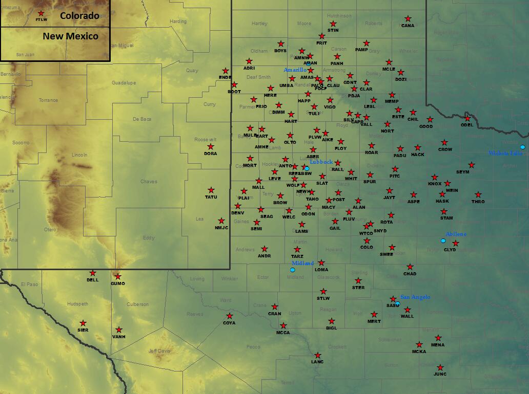
A deep learning neural network was designed which takes historical wind speed, wind direction, temperature, humidity, pressure, dew point and solar radiation as inputs to predict future short-term wind speed. The reason for employing multiple meteorological variables as inputs is they could improve the accuracy of wind prediction [11]. Even more, for some situation the prediction uncertainty depends on weather condition such as pressure [12]. Considering this, we incorporate multiple meteorological variables and propose a stacked long-short term memory network to learn these complex interactions for short-term wind speed forecasting. Extensive experiments were implemented to verified the model using real data from West Texas Mesonet Stations, as shown in Figure 1. Different from previous work, this paper targets at wind speed forecasting at every five minutes.
II Wind Speed Forecasting Model
The most challenging part of wind speed forecasting lies in its real-time dynamics, therefore, in this paper we decide to utilize LSTM model for wind speed forecasting due to its well-handling of long and short term time dependency [9]. LSTM shows its superiority over the traditional recurrent neural network method. Therefore, we choose deep learning neural networks with LSTM in the hidden layer in this paper to predict wind speed. Figure 2(b) shows the basic structure of LSTM. It has an input gate , output gate , forget gate and memory cell . Equations (1) to (5) shows how to update the output values each step[13]. is the input vector and is the activation function such as ReLU or Sigmoid function. is the weight vector. We used ReLU in this paper because it will not have the problem of Vanishing Gradient and converge quickly.
| (1) |
| (2) |
| (3) |
| (4) |
| (5) |
Figure 2(c) presents the framework of the proposed MSLSTM model. After the input layer, there are two LSTM layers stacked together before forwarding to a Dropout and a Dense layer at the final output. The first LSTM layer produces sequence vectors which will be used as the input of the subsequent LSTM layer. In addition, the LSTM layer receives feedback from its previous time step thus can capture certain patterns. In other words, this hierarchy helps the network to enable more complex representation of the wind speed time series data, and captures information at different scales. The Dropout layer excludes 5% of the neurons to avoid over-fitting. The proposed MSLSTM model ingests multiple meteorological variables, including Wind speed, wind direction, temperature, humidity, pressure, dew point, wind speed at two meters high and solar radiation. The deep learning neural networks could extract the hidden patterns from these variables and predict wind speed.

III Experimental results
III-A Dataset
Multiple meteorological variables are used as inputs to improve the accuracy of wind prediction because there exists some correlations between different meteorological variables [11, 12]. Table I lists the correlation between wind speed and other variables. Wind direction, temperature, solar radiation, wind speed at 2 meters shows strong correlation with wind speed (wind speed at 10 m). Other factors such as humidity and dew point also show relative high correlation with wind speed.
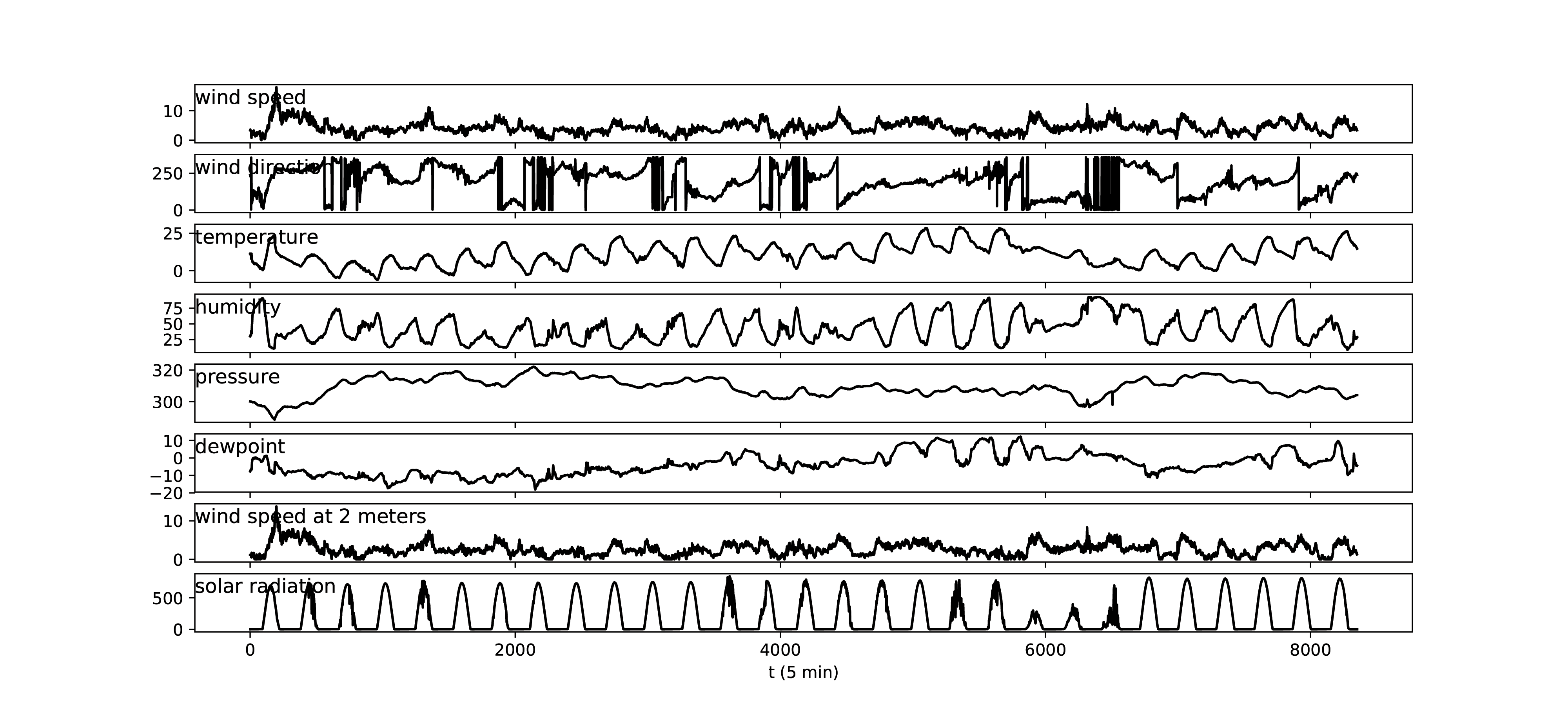
The dataset used in this paper was collected by West Texas Mesonet [10]. The whole dataset includes data collected in 2016 from 117 weather stations, spreading out in West Texas. Figure 3 shows a data sample that are collected with 5-min intervals from one weather station. As shown in the table, every record in the dataset has eight weather attributes (wind speed at 10 meters, wind direction, temperature, humidity, pressure, dew point, wind speed at 2 meters, solar radiation ).
| Correlation | p-value | |
|---|---|---|
| Wind Direction | -0.1173* | 0.0105 |
| Temperature | -0.1079* | 0.0186 |
| Humidity | -0.0524 | 0.2542 |
| Pressure | -0.0050 | 0.9133 |
| Dewpoint | -0.1021 | 0.0261 |
| Wind speed at 2 meters | -0.2719* | 1.7064e-09 |
| Solar Radiation | 0.2515* | 2.7462e-08 |
III-B Data Preprocessing
The data preprocessing part includes normalization and handling missing data. If there are some missing values, the corresponding records were simply deleted. The normalization is to make the input meteorological variables share the same structures and time scales. Normalized data is computed as: , where is normalized value for time . is the maximum value of all the data for one feature. is real value at time . is the minimum value of all the data for one feature. Wind speed, wind direction, temperature, humidity, pressure, dew point, solar radiation are all normalized to 0-1 by the above equation.
III-C Implementation
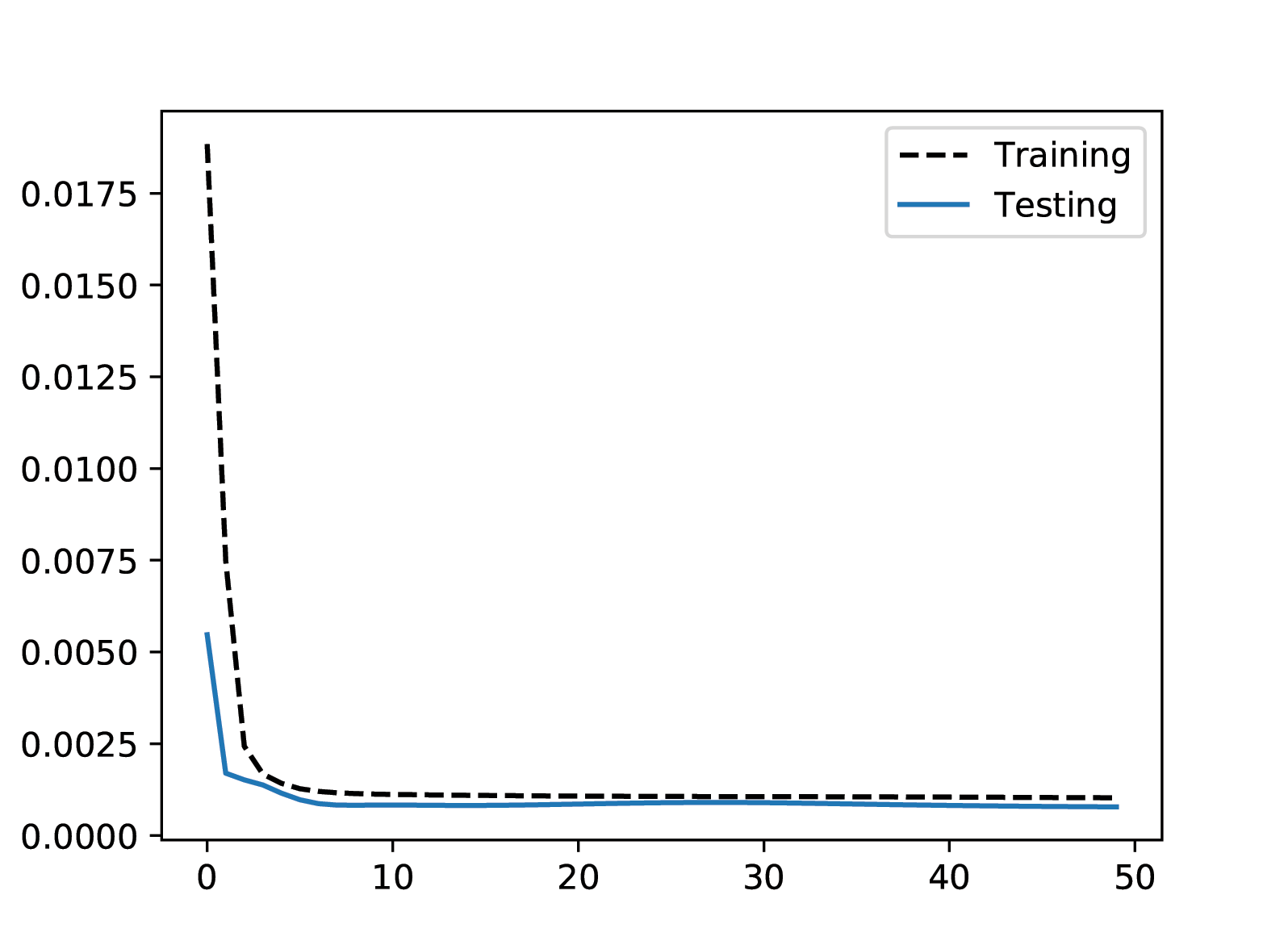
The model is implemented in python with keras package which utilized Tensorflow as backend. The code is executed in a desktop with Nvidia GTX970 graphics card and i7-6700 CPU. The batch size is 40 and training epochs are 50. MSE was defined as the loss function. The loss changes of training and test process was plotted in Figure 4. The loss of testing process is close to the loss of training process.


III-D Evaluation Matrix
Mean square error (MSE), root mean square error (RMSE) and mean absolute error (MAE) are employed to evaluate the performance of the models. denotes the real value at time t and is the predicted value at time t. is the total number of sample cycle. The MSE, RMSE and MAE values are calculated base on the following equations: , and .
III-E Numeric Results
To verify the effectiveness of the proposed MSLSTM model, we compare the forecasting performance with multiple competing methods, including Multiple Linear Regression, LASSO, Ridge and LSTM model. The performance assessment and results shown in this paper are based on one-month data collected at Andrew in February 2016. It contains one-month data which sampled at 5-min intervals and has a total length of 8353 points. For training dataset, we randomly took 90 percent from the whole dataset, and the rest was used for testing.
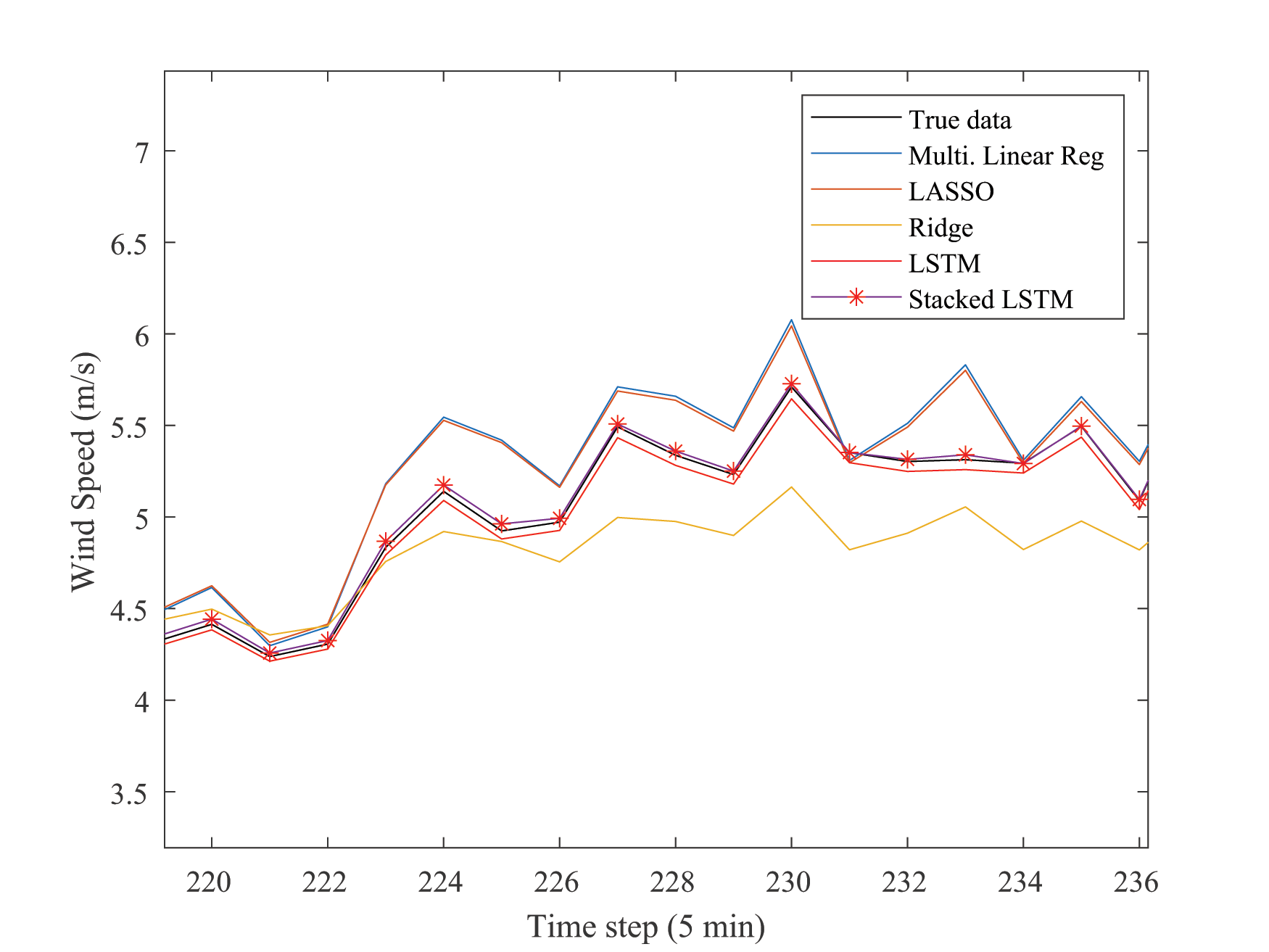
Figure 5 depicts a small piece of wind speed prediction results on sample data, where we can see conventional prediction models are far away from true data, and both LSTM and MSLSTM stick to the ground truths. Multiple Linear Regression and Lasso regression have similar results which predict higher wind speed, while Ridge regression tends to have a lower wind speed. Table II illustrates the performance of different models under MSE, RSME and MAE matrix. We also compute statistics on each model, where MSLSTM has the highest value of that confirms its superiority over all the baselines. As shown in Table II, the evaluation results of MSE, RMSE and MAE demonstrate the stacked LSTM consistently outperforms the rest models.
| MSE | RMSE | MAE | ||
|---|---|---|---|---|
| Multi. Linear Reg. | 0.22227 | 0.47146 | 0.37485 | 0.93750 |
| Lasso | 0.20887 | 0.45703 | 0.36460 | 0.94127 |
| Ridge | 0.88995 | 0.94337 | 0.73796 | 0.74979 |
| LSTM | 0.01107 | 0.10522 | 0.07988 | 0.99689 |
| Stacked LSTMs | 0.00297 | 0.05448 | 0.04275 | 0.99917 |
IV conclusion
This paper proposed a multi-variable stacked LSTMs model to predict short-term wind speed. This model allows multiple meteorological parameters ingestion for real-time wind forecasting. The proposed MSLSTM model helps the network to enable a more complex representation of the wind speed time series data, and captures information at different scales from historical parameters, at the same time prevents over-fitting. All in all, the deep MSLSTM model could extract features from all the input variables which improved the precision of the prediction. MSE, RMSE, MAE and evaluation results indicate that MSLSTM outperformed other competing methods consistently. This paper uses modern machine learning techniques for short-term wind speed forecasting with extracting patterns from so many meteorological variables, and successfully learn many effective features than traditional methods, which could inspire new applications in meteorology.
Acknowledgment
This work was supported by the U.S. National Science Foundation under Grant CNS-1737634. The authors would like to thank West Texas Mesonet, Dr. John Schroeder and Mr. Wes Burget for providing weather data in this paper.
References
- [1] J. L. Sawin, J. Rutovitz, F. Sverrisson et al., “Renewables 2018 global status report,” 2018.
- [2] S. Buhan, Y. Özkazanç, and I. Çadırcı, “Wind pattern recognition and reference wind mast data correlations with nwp for improved wind-electric power forecasts,” IEEE Transactions on Industrial Informatics, vol. 12, no. 3, pp. 991–1004, 2016.
- [3] S. Fang and H.-D. Chiang, “A high-accuracy wind power forecasting model,” IEEE Transactions on Power Systems, vol. 32, no. 2, pp. 1589–1590, 2017.
- [4] K. Bhaskar and S. Singh, “Awnn-assisted wind power forecasting using feed-forward neural network,” IEEE transactions on sustainable energy, vol. 3, no. 2, pp. 306–315, 2012.
- [5] S. S. Soman, H. Zareipour, O. Malik, and P. Mandal, “A review of wind power and wind speed forecasting methods with different time horizons,” in North American power symposium (NAPS), 2010. IEEE, 2010, pp. 1–8.
- [6] J. Jung and R. P. Broadwater, “Current status and future advances for wind speed and power forecasting,” Renewable and Sustainable Energy Reviews, vol. 31, pp. 762–777, 2014.
- [7] M. Khodayar and J. Wang, “Spatio-temporal graph deep neural network for short-term wind speed forecasting,” IEEE Transactions on Sustainable Energy, 2018.
- [8] H. Wang, G. Wang, G. Li, J. Peng, and Y. Liu, “Deep belief network based deterministic and probabilistic wind speed forecasting approach,” Applied Energy, vol. 182, pp. 80–93, 2016.
- [9] S. Hochreiter and J. Schmidhuber, “Long short-term memory,” Neural computation, vol. 9, no. 8, pp. 1735–1780, 1997.
- [10] texas tech national wind institute. (2018, Oct.) West texas mesonet. [Online]. Available: http://www.mesonet.ttu.edu
- [11] H. Geerts, “Short range prediction of wind speeds: a system-theoretic approach,” in Proceedings of the European Wind Energy Conference, Hamburg (DE), 1984, pp. 594–599.
- [12] M. Lange and H.-P. Waldl, “Assessing the uncertainty of wind power predictions with regard to specific weather situations,” in Proceedings of the European Wind Energy Conference, Copenhagen, Denmark, 2001, pp. 695–698.
- [13] L. H. Nguyen, R. Hewett, A. S. Namin, N. Alvarez, C. Bradatan, and F. Jin, “Smart and connected water resource management via social media and community engagement,” in 2018 IEEE/ACM International Conference on Advances in Social Networks Analysis and Mining (ASONAM), Aug 2018, pp. 613–616.