Streaming Generalized Cross Entropy

Abstract.

We propose a new method to combine adaptive processes with a class of entropy estimators for the case of streams of data.

Starting from a first estimation obtained from a batch of initial data, model parameters are estimated at each step by combining the prior knowledge with the new observation (or a block of observations). This allows to extend the maximum entropy technique to a dynamical setting, also distinguishing between entropic contributions of the signal and the error. Furthermore, it provides a suitable approximation of standard GME problems when the exacted solutions are hard to evaluate.

We test this method by performing numerical simulations at various sample sizes and batch dimensions. Moreover, we extend this analysis exploring intermediate cases between streaming GCE and standard GCE, i.e. considering blocks of observations of different sizes to update the estimates, and incorporating collinearity effects as well. The role of time in the balance between entropic contributions of signal and errors is further explored considering a variation of the Streaming GCE algorithm, namely, Weighted Streaming GCE. Finally, we discuss the results: in particular, we highlight the main characteristics of this method, the range of application, and future perspectives.

University of Salento¹ and sezione INFN²,

Lecce, 73100, Italy

Keywords: Generalized Maximum Entropy, streaming data, adaptive process
MSC[2010] 94A17, 62Jxx, 62L12

1. Introduction

Several situations in modern research and technological development have an essential time directionality, which arises from a sequential acquisition of the data while producing outputs and decisions at intermediate steps.

Concrete examples of this feature include the update of control parameters in dynamical systems (mobile phones, GPS), social networks, image analysis, economic analysis (cryptocurrency), as well as longitudinal studies in the social sciences or psychological change occurring over time during the psychoterapeutic process, etc. These data may be characterized by

• large sample size (e.g., big data);

• unstructured data (e.g., audio/video, natural language);

• the need of a continuous, streaming analysis (e.g., image analysis);

• the need for fast answer/output given a new input (e.g., submarine robot control).

These aspects show many drawbacks in concrete applications, because standard analyses on whole dataset:

• are computationally expensive, as they require the whole algorithm to run at each new observation;

• hide the relationship between subsequent estimates at consecutive times $i\rightarrow i+1$ and, hence, the information acquisition and knowledge dynamics;

• may fail to provide prompt responses, and have to be adapted to work in real time with online data.

Therefore, in these situations, one cannot disregard the role of the time flow. The process itself has to flexibly adapt to the evolution of the system.

In order to highlight the temporal structure of the data, we will make use of the Maximum Entropy Principle (MEP), which allows to extract the essential information available in a set of observations with the least amount of additional assumptions. The MEP is a cornerstone in contemporary science due to its capacity to embed either quantitative or qualitative aspects of information within models for a variety of applications and, hence, connect several different frameworks: nowadays, applications of the MEP can be found in artificial intelligence (Solomonoff’s universal inductive reasoning [1]), complexity theory [2], linguistics [3], biology [4] etc.

A remarkable development of the MEP in statistical regression is given by the Generalized Maximum Entropy (GME) approach [5, 6, 7], which is successfully employed to provide estimates of both parameters and errors in regression models. The extension to multivariate analysis has been developed in the last decade [8, 9]. These techniques proved to be useful in psychological and social studies on both perception and satisfaction [10, 11], in the analysis of observational studies [12] and also in combination with Structural Equation Models (SEM) [13, 14, 15].

On another hand, as the implementation of the GME method involves a whole dataset, there is a permutation symmetry for the consistency constraints: in this context, the implications of the temporal dimension are lost.

The aim of the present work is to investigate the combination of the information theory based on the GME and adaptive aspects during a streaming flow of data. This purpose entails a natural distinction between the parameters of the model, which represent the “recurrent” part of the set of observations, and errors, which represent the “accidental” part. The parameters, which will also be referred to as the signal, are iteratively estimated from upcoming new data, while the errors are necessary to make the recurrent part consistent with different instances of the underlying model. Further insight on the above-mentioned components is evident when observing their natural evolution over a stream of data.

In order to explore such distinction, we consider an adaptive process and update the probability distributions associated with both the signal and the errors. We choose the cross entropy (or Kullback-Leibler divergence) as cost function to be minimized at each step, under the constraints given by the new data in the stream. The asymmetry between the signal and the error is represented by different priors associated to each one of them in the cross entropy. These two notions, —adaptive evolution during a stream and entropy-based principle to combine prior information and new data —are the roots of the Streaming Generalized Cross Entropy (Stre-GCE) presented in this work.

The inclusion of the temporal aspect can be used to explore the dynamics of the parameter estimation when new data come up: indeed, the temporal factor can be used to interpolate the partial information represented by a data subset (the batch) and the full information provided by the whole sample: the update of the weights associated to both the already existing and the upcoming information over time will be the focus of the extension of the Stre-GCE algorithm called Weighted Stre-GCE.

The paper is organized as follows: in Section 2, we provide a basic definition of our algorithm by briefly mentioning adaptive process and the standard GCE method in linear regression. The description of the Stre-GCE method, the regime where it is considered, its analogies and differences with respect to the GME and GCE techniques are discussed in Section 3. Section 4 is devoted to the formalization of the Stre-GCE algorithm. In order to compare the performance of Stre-GCE with respect to GME and simple GCE, we run a set of simulations that are discussed in Section 5. In particular, we focus on the comparison between Root Mean Square Errors (RMSE), we extend Stre-GCE beyond the single-unit update to a stream of blocks of data, and we explore multicollinearity effects. In Section 6, we extend the basic Stre-GCE algorithm so that the relation between the signal and the error contributions evolves during the data stream. Results of these simulations are discussed in detail in Section 7, while future perspectives and applications of Stre-GCE are suggested in Section 8.

2. Preliminaries

The implementation of the Stre-GCE algorithm requires two main “ingredients”: adaptive processes and the Generalized Cross Entropy method.

2.1. Adaptive processes

When a model evolves over time, the role of all the agents should be taken into account (e.g. the actions of the observer, the decisions made consistently with the previously processed data). Inclusion of flow of information along with a sequence of control steps in the same framework leads to an adaptive process in which previous outputs and new data are merged together based on a given criterion. Such a criterion is often quantified by a cost (or reward) function, that is, a measure of the discrepancy between the actual model and a “more favorable” one, in accordance with the new data. Applications include, but are not limited to, system and control theory [16] pattern recognition [17], and reinforcement learning [18].

A major example of adaptive process is the Kalman Filter (KF), a fundamental tool in control theory [16]. The standard Kalman filter takes advantage from the linearity of the model and the Gaussian distribution of errors at its roots. Consequently, one can consider algebraic formulations based on Least Squares (LS) methods in order to provide exact formulas for optimal estimation. The Recursive Least Squares (RLS) algorithm fills the need of an efficient inclusion of new data in the model.

However, the efficacy of this method is limited by the same assumptions mentioned before. Nonlinear models and multimodal distributions make the implementation of the standard Kalman filter ineffective [16, 19]. This drastically impacts on decision theory, where non-trivial symmetries may relate different states or transitions, and the standard Kalman filter does not faithfully represent this ambiguity. An efficient application of the KF in relation to its optimality properties among linear estimators only relies on the exact knowledge of covariance matrices for errors: however, this condition is hardly fulfilled in concrete situations.

For these reasons, nonlinear extensions of the Kalman filter have been developed (e.g. extended KF, unscented KF, particle filters), as well as additional numerical methods (see [20]). Even though each of these approaches returns some information on the required probability distribution with greater generality, they are often computationally expensive and rely on recursive schemes for approximations [20, 19], thus being unsuitable for real-time data.

Besides statistical assumptions, KF and several other methods in linear models depend on specific algebraic hypotheses, which reflect on the observability of the system: these requirements are not fulfilled in presence of multicollinearity or when numerical approximations lead to rank reductions. Multicollinearity can be managed with other approaches (see e.g. [21] for an analysis of performance of regression methods under multicollinearity), including the GME and GCE methods that are summarized in the following subsections.

2.2. Generalized Cross Entropy (GCE)

The notion of entropy arose in early works by Boltzmann, Gibbs and Planck in statistical mechanics, where the equilibrium state in a macroscopic system is represented by the maximum entropy distribution compatible with macroscopic observables [22, 23], and by Shannon in the analysis of optimal communication information theory (see [24] for a review). The key aspects of the Maximum Entropy Principle (MEP) have been intensively explored by Khinchin [25], Kullback and Leibler and Jaynes, in order to identify its characterizing features that do not rely on the specific physical system [26] and, hence, make it a fundamental principle for inference [27]. A number of distinctive features of the MEP can be also drawn in relation to other methods, such as Maximum Likelihood, Empirical Likelihood, Bayesian method of moments and (ordinary or weighted) Least Squares [28].

For our purposes, GME and GCE approaches for regression models play a relevant role [5, 6, 7]. In particular, we focus on linear regression

$$\mathbf{y}=\boldsymbol{\beta}\cdot\mathbf{x}+\boldsymbol{\varepsilon}$$ (2.1)

involving a set of $n$ units

$$y_{i}=\sum_{j=1}^{J}\beta_{j}\cdot x_{i,j}+\varepsilon_{i},\quad i\in\{1,\dots,n\},$$ (2.2)

Through GME, one can express both the parameters $\beta_{j}$, $j\in\{1,\dots,J\}$ (and, possibly, the intercept $\alpha$) and the errors $\varepsilon_{i}$, $i\in\{1,\dots,n\}$, as expected values with respect to a certain probability distribution $\left(\mathbf{p}^{\beta_{1}},\dots,\mathbf{p}^{\beta_{J}},\mathbf{p}_{1}^{\varepsilon},\dots,\mathbf{p}_{n}^{\varepsilon}\right)$ supported on a finite set. Specifically, $K$ is the number of support points $\{z_{j,k}^{\beta}:\,k\in\{1,\dots,K\}\}$ for $\beta_{j}$ and $H$ is the number of support points $\{z_{i,h}^{\varepsilon}:\,h\in\{1,\dots,H\}\}$ for $\varepsilon_{i}$. So (2.2) can be restated as a set of $n$ constraints

$$y_{i}=\sum_{j=1}^{J}\sum_{k=1}^{K}p_{j,k}^{\beta}\cdot z_{j,k}^{\beta}\cdot x_{i,j}+\sum_{h=1}^{H}p_{i,h}^{\varepsilon}\cdot z_{i,h}^{\varepsilon},\quad i\in\{1,\dots,n\}$$ (2.3)

with

$$\sum_{k=1}^{K}p_{j,k}^{\beta}=\sum_{h=1}^{H}p_{i,h}^{\varepsilon}=1,\quad j\in\{1,\dots,J\},\,i\in\{1,\dots,n\}.$$ (2.4)

In matricial terms, (2.3)-(2.4) can be expressed as

$$\mathbf{y}_{n\times 1}= \mathbf{X}_{n\times J}\cdot\mathrm{diag}(\mathbf{Z}_{J\times K}^{\beta}\cdot(\mathbf{P}_{J\times K}^{\beta})^{T})_{J\times 1}+\mathbf{P}_{n\times H}^{\varepsilon}\cdot\mathbf{z}_{H\times 1}^{\varepsilon},$$

$$\mathbf{1}_{J\times 1}= \mathbf{P}_{J\times K}^{\beta}\cdot\mathbf{1}_{K\times 1},$$

$$\mathbf{1}_{n\times 1}= \mathbf{P}_{n\times H}^{\varepsilon}\cdot\mathbf{1}_{H\times 1}$$

where the dimensions of each matrix are made explicit in the corresponding suffix. For any natural numbers $a$ and $b$, $\mathrm{diag}(\mathbf{M}_{a\times a})$ is the $(a\times 1)$-dimensional matrix (a column vector) whose entries are the diagonal entries of $\mathbf{M}$, and $\mathbf{1}_{a\times b}$ is the $(a\times b)$-dimensional matrix with all entries equal to $1$. The maximization of Shannon’s entropy

$$H\left(\mathbf{p}^{\beta_{1}},\dots,\mathbf{p}^{\beta_{J}},\mathbf{p}_{1}^{\varepsilon},\dots,\mathbf{p}_{n}^{\varepsilon}\right)=-\sum_{j=1}^{J}\sum_{k=1}^{K}p_{j,k}^{\beta}\cdot\ln p_{j,k}^{\beta}-\sum_{i=1}^{n}\sum_{h=1}^{H}p_{i,h}^{\varepsilon}\cdot\ln p_{i,h}^{\varepsilon}$$ (2.5)

subject to consistency (2.3) and normalization (2.4) constraints returns a highly accurate estimation of the parameter and the error terms. Note that the components of the joint distribution $\left(\mathbf{p}^{\beta_{1}},\dots,\mathbf{p}^{\beta_{J}},\mathbf{p}_{1}^{\varepsilon},\dots,\mathbf{p}_{n}^{\varepsilon}\right)$ are assumed to be independent, as it can be seen from the form of Shannon’s entropy (2.5). In particular, we can write $H\left(\mathbf{p}^{\beta_{1}},\dots,\mathbf{p}^{\beta_{J}},\mathbf{p}_{1}^{\varepsilon},\dots,\mathbf{p}_{n}^{\varepsilon}\right)=H\left(\mathbf{p}^{\beta_{1}},\dots,\mathbf{p}^{\beta_{J}}\right)+H\left(\mathbf{p}_{1}^{\varepsilon},\dots,\mathbf{p}_{n}^{\varepsilon}\right)$, where

$$H\left(\mathbf{p}^{\beta_{1}},\dots,\mathbf{p}^{\beta_{J}}\right) := -\sum_{j=1}^{J}\sum_{k=1}^{K}p_{j,k}^{\beta}\cdot\ln p_{j,k}^{\beta},$$

$$H\left(\mathbf{p}_{1}^{\varepsilon},\dots,\mathbf{p}_{n}^{\varepsilon}\right) := -\sum_{i=1}^{n}\sum_{h=1}^{H}p_{i,h}^{\varepsilon}\cdot\ln p_{i,h}^{\varepsilon}.$$

It is worth stressing that the errors $\varepsilon_{i}$ make the problem (2.3) under-conditioned for a generic choice of $J$ and $n$, as the number of unknowns in the distribution is larger than the number of constraints. For this reason, a criterion (such as the entropy maximization) is needed in order to select a single probability distribution among several ones that satisfy both consistency and normalization constraints.

In order to compare different models represented by two distributions $\mathbf{q}$ and $\mathbf{p}$ on a set $\Omega$, a generalization of Shannon’s entropy can be worthwhile. This can be achieved by introducing the cross entropy (or Kullback-Leibler divergence) from $\mathbf{q}$ to a dominated distribution $\mathbf{p}$, which is defined by

$$\mathrm{D_{KL}}(\mathbf{p}||\mathbf{q}):=\sum_{\alpha\in\Omega}p_{\alpha}\cdot\log\left(\frac{p_{\alpha}}{q_{\alpha}}\right).$$ (2.6)

Here, the symbol “$:=$” denotes the introduction of a mathematical entity (in this case, the cross entropy function) through a definition. We also stress out that (2.6) is defined even when some of the components of $\mathbf{p}$ vanish; in other words, it is defined in the whole ($|\Omega|-1$)-dimensional probability symplex. In this regard, since events with zero probability do not contribute to the cross entropy, we assume the identity $0\cdot\log 0=0$. A similar argument holds for (2.5).

The cross entropy formalizes a notion of “distance” between $\mathbf{p}$ and an initial distribution $\mathbf{q}$. Whenever $\mathbf{q}$ is the uniform distribution $\mathbf{u}$ over a fixed finite set $\Omega=\{\alpha_{1},\dots,\alpha_{n}\}$, one finds that $\mathrm{D_{KL}}(\mathbf{p}||\mathbf{u})=n-H(\mathbf{p})$, where the entropy $H(\mathbf{p})$ associated with $\mathbf{p}$ is $-\sum_{\alpha\in\Omega}p_{\alpha}\cdot\log p_{\alpha}$. Therefore, the minimization of $\mathrm{D_{KL}}$ reduces to the maximum entropy approach. For our purposes, the distribution $\mathbf{q}$ can be regarded as a way to encode the prior information, and the cross entropy provides us with an adequate tool to track the dynamics of the model.

Using the cross entropy as objective function to be minimized, one can extend the GME to the Generalized Cross Entropy (GCE) approach. Introducing the notation $\mathbb{I}:=[0;1]$, this translates into the minimization of the objective function

$$\underset{{\scriptstyle\mathbb{I}^{JK}\times\mathbb{I}^{nH}}}{\mathrm{argmin}}\mathrm{D_{KL}}\left(\left(\mathbf{p}^{\beta_{1}},\dots,\mathbf{p}^{\beta_{J}},\mathbf{p}_{1}^{\varepsilon},\dots,\mathbf{p}_{n}^{\varepsilon}\right)||\left(\mathbf{q}^{\beta_{1}},\dots,\mathbf{q}^{\beta_{J}},\mathbf{q}_{1}^{\varepsilon},\dots,\mathbf{q}_{n}^{\varepsilon}\right)\right)$$ (2.7)

$$= \underset{{\scriptstyle\mathbb{I}^{JK}\times\mathbb{I}^{nH}}}{\mathrm{argmin}}\left(\sum_{j=1}^{J}\sum_{k=1}^{K}p_{j,k}^{\beta}\ln\left(\frac{p_{j,k}^{\beta}}{q_{j,k}^{\beta}}\right)+\sum_{i=1}^{n}\sum_{h=1}^{H}p_{i,h}^{\varepsilon}\ln\left(\frac{p_{i,h}^{\varepsilon}}{q_{i,h}^{\varepsilon}}\right)\right)$$

where the optimization is conducted with respect to the distribution $(\mathbf{p}^{\beta_{1}},\dots,$ $\mathbf{p}^{\beta_{J}},\mathbf{p}_{1}^{\varepsilon},\dots,\mathbf{p}_{n}^{\varepsilon})$ under the same constraints (2.3) and (2.4).

Concrete applications of GME and GCE methods could be hard to implement: a computationally expensive optimization procedure, along with a slow processing of real-time data and the general shortcomings of “global” techniques, make their implementation often unfeasible. Furthermore, on a conceptual ground, time effects get lost in these approaches.

3. Characteristics and range of application of Stre-GCE

Before moving to the algorithm definition and the analysis of its performance via simulations, we discuss the characteristics of the Stre-GCE method in light of the issues mentioned in previous sections.

First, the consistency constraints and the temporal dimension can be both preserved through the relaxation of the GME method. Specifically, the standard GCE with uniform prior involves the whole set of constraints (2.3), while a time-sensitive acquisition of information follows from subsequent upgrades of the distribution $(\mathbf{p}^{\beta_{1}},\dots,\mathbf{p}^{\beta_{J}})$ via a step-by-step introduction of constraints: only the $i^{\mathrm{th}}$ equation (2.2) is strictly satisfied at the $i^{\mathrm{th}}$ step. However, constraints at previous steps affect the computation through the objective function: this leads us to choose the cross entropy to move from a prior distribution to a posterior one as new data show up.

It is worth to note that, in contrast with the standard GCE method, our definition of the prior does not rely on information which is external to the dataset:

• we start from a uniform distribution on the supports of parameters and errors, and provide a first prior evaluation based on a batch of initial data;

• the model is updated by incorporating new information to the prior. This adaptive step involves the updating of both the estimates and the prior.

Therefore, one can see that the prior does not encode knowledge external to the process, but it allows us to identify the temporal aspects of data acquisition. To this extent, Stre-GCE is sensitive to the time flow, hence it can be used when irreversibility plays a relevant role.

Such a relaxation also leads to computational advantages, as it allows to move from a constrained problem with $n$ consistency conditions to $n$ problems, each made up of a single condition. This way, a solution to new problems can be found even when the original problem is computationally unmanageable with the available softwares. The splitting strategy can be modified in order to get intermediate cases between Stre-GCE and standard GME/GCE: instead of individual observations, we can consider the data received within a given time frame. Processing partitions of the set of units $\{1,\dots,n\}$ in pairwise disjoint subsets $\mathcal{N}_{1},\dots,\mathcal{N}_{g}$, e.g. intervals, such that $\bigcup_{\ell=1}^{g}\mathcal{N}_{\ell}=\{1,\dots,n\}$, allows us to infer parameters and errors through consecutive applications of GCE method within each individual time window. For $g=1$, one has the original GCE problem with uniform prior, while at $g=n$ one recovers the Stre-GCE. The steps in between will be referred to as “block Stre-GCE”.

Looking at the dual (or compressed) problem, the difference between the two extreme solutions (GCE with uniform prior and Stre-GCE) can be identified through the Lagrange multipliers that optimise the respective objective functions. These multipliers allow the natural weights involved in empirical likelihood techniques (see e.g. [28]) to change as the sequential inclusion of constraints progresses. On the computational side, there are $J$ equations in the dual problem, each of which is associated with a parameter $\beta_{j}$, $j\in\{1,\dots,J\}$. In several applications, $J$ is smaller than the number of units $n$ and, in any case, it is fixed for a given model. However, in order to recover a solution from the minimization of the dual function (that is the free energy or Legendre transform of the entropy), one has to evaluate all the Lagrange multipliers associated with the constraints (2.3). Depending on the available methods for the evaluation and the number of parameters and observations, this task can still be difficult to accomplish. Moreover, such a formulation cannot be applied exactly when one considers a more general class of nonlinear (and, in particular, non-convex) optimization problems when the equivalence of the two formulations (strong duality) does not hold. Indeed, alternative methods and approximations are studied to overcome this problem and get (pseudo-)optimal solutions [29].

On the other hand, the Stre-GCE relaxation through subsequent updates of estimations is manageable from both the primal and the dual perspectives. Similarly to Recursive Least Squares (RLS) algorithms and the Kalman Filter [16], these methods result into faster computations as only partial information has to be managed at intermediate times.

Finally, we remark a conceptual shift from GCE with uniform prior to Stre-GCE: we get an intrinsic method to assign different roles to signal and error. Other approaches usually claim for external parameters to be added, whose evaluation is based on given optimization criteria [30]. On the contrary, Stre-GCE estimates the different entropic contributions for both the signal and error as they evolve in time, without the need of any additional variable: in Stre-GCE, the prior for signal is sensitive to time evolution, while the prior for error is identically uniform. Consequently, it is possible to look at how the information evolves at intermediate times in terms of the entropy production, which is a fundamental concept in nonequilibrium processes [31, 32]. We will focus on this issue in a separate work.

4. Stre-GCE algorithm

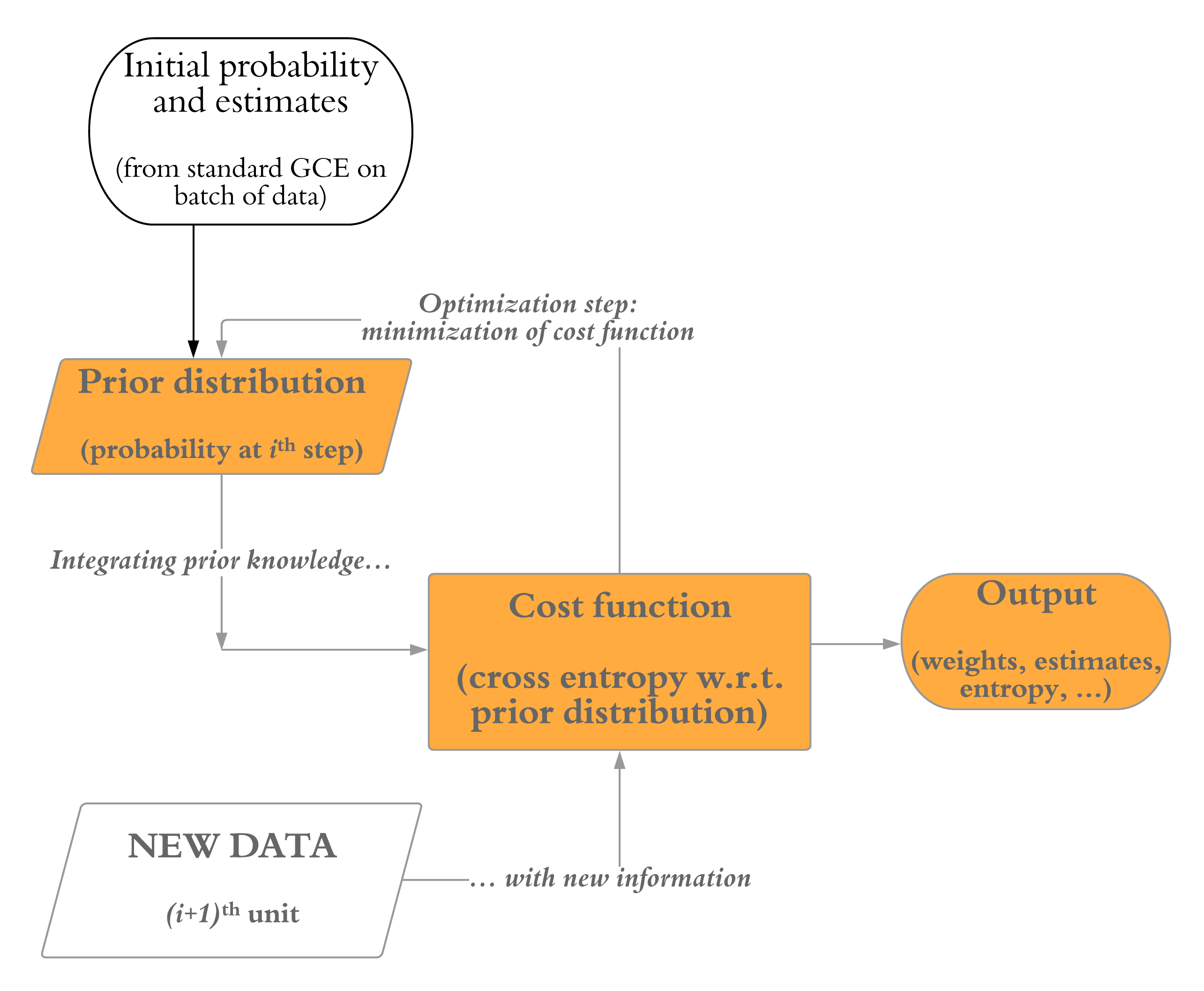
The previous discussion can be formalized in the scheme pictured in Figure 4.1. This is the basis for the Stre-GCE algorithm, formally implemented in this section.

Figure 4.1. Scheme of the Stre-GCE algorithm.

Initial step

We start from an initial situation where a number $m$ of consistency constraints, with $m<n$, have been collected. This provides us with a batch from which the initial estimates can be obtained. Specifically, we can get

$$\hat{\beta}_{j}^{(m)} := \sum_{k=1}^{K}\hat{p}_{j,k}^{\beta(m)}\cdot z_{j,k}^{\beta},\quad j\in\{1,\dots,J\},$$

$$\hat{\varepsilon}_{i} := \sum_{h=1}^{H}\hat{p}_{i,h}^{\varepsilon}\cdot z_{i,h}^{\varepsilon},\quad i\in\{1,\dots,m\}$$ (4.1)

through the GCE method with uniform prior. As already mentioned, this choice of the prior leads to the equivalence with the standard GME from the optimization view, so this approach selects the probability distribution

$$(\mathbf{\hat{P}}^{\beta(m)},\mathbf{\hat{p}}_{1}^{\varepsilon},\dots,\mathbf{\hat{p}}_{m}^{\varepsilon}) := \underset{{\scriptstyle\mathbb{I}^{JK}\times\mathbb{I}^{mH}}}{\mathrm{argmin}}\mathrm{D_{KL}}\left((\mathbf{P}^{\beta},\mathbf{p}_{1}^{\varepsilon},\dots,\mathbf{p}_{m}^{\varepsilon})||(\mathbf{U}^{\beta},\mathbf{u}^{\varepsilon},\dots,\mathbf{u}^{\varepsilon})\right)$$

$$= \underset{{\scriptstyle\mathbb{I}^{JK}\times\mathbb{I}^{mH}}}{\mathrm{argmax}}\left(H(\mathbf{P}^{\beta})+\sum_{i=1}^{m}H(\mathbf{p}_{i}^{\varepsilon})\right)$$

$$= \underset{{\scriptstyle\mathbb{I}^{JK}\times\mathbb{I}^{mH}}}{\mathrm{argmax}}\left(-\sum_{j=1}^{J}\sum_{k=1}^{K}p_{j,k}^{\beta}\cdot\ln p_{j,k}^{\beta}-\sum_{h=1}^{H}\sum_{i=1}^{m}p_{i,h}^{\varepsilon}\cdot\ln p_{i,h}^{\varepsilon}\right)$$

where the choice set is the set of all the distributions $(\mathbf{P}^{\beta},\mathbf{p}_{1}^{\varepsilon},\dots,\mathbf{p}_{m}^{\varepsilon})$ satisfying the constraints

$$\left\{\begin{array}[]{c}{\displaystyle y_{i}=\sum_{j=1}^{J}\sum_{k=1}^{K}p_{j,k}^{\beta}\cdot z_{j,k}^{\beta}\cdot x_{i,j}+\sum_{h=1}^{H}p_{i,h}^{\varepsilon}z_{i,h}^{\varepsilon}},\quad i\in\{1,\dots,m\}\\ {\displaystyle\sum_{k=1}^{K}p_{j,k}^{\beta}=\sum_{h=1}^{H}p_{i,h}^{\varepsilon}=1,\quad j\in\{1,\dots,J\},\,i\in\{1,\dots,m\}}\end{array}\right..$$ (4.3)

From the method of Lagrange multipliers associated with these linear constraints, one gets the weights of Gibbs’ type (see e.g. [22, 7] for more details)

$$\hat{p}_{j,k}^{\beta(m)} = \frac{1}{Z_{j}^{\beta(m)}}\cdot\exp\left(-z_{j,k}^{\beta}\cdot\sum_{i=1}^{m}x_{i,j}\hat{\lambda}_{i}\right),\quad j\in\{1,\dots,J\},\,k\in\{1,\dots,K\},$$

$$\hat{p}_{i,h}^{\varepsilon} = \frac{1}{Z_{i}^{\varepsilon}}\cdot\exp\left(-z_{i,h}^{\varepsilon}\hat{\lambda}_{i}\right),\quad i\in\{1,\dots,m\},\,h\in\{1,\dots,H\}.$$ (4.4)

where the multipliers $\hat{\lambda}_{i}$ are chosen in order to get (2.2) and the normalizing factors $Z_{j}^{\beta(m)}$, $Z_{i}^{\varepsilon}$ ensure that (2.4) holds.

Update step: $i\rightarrow i+1$

In the update process, the actual estimates for signal and error are combined with the new observation in order to produce a new estimate. This purpose is attained through the minimization of the cross entropy (or Kullback-Leibler divergence) $\mathrm{D_{KL}}((\mathbf{P}_{i+1}^{\beta},\mathbf{p}_{i+1}^{\varepsilon})||(\mathbf{\hat{P}}_{i}^{\beta},\mathbf{u}_{i}^{\varepsilon}))$. The asymmetry between signal and error is naturally expressed by different priors for $\mathbf{P}^{\beta}$ and $\mathbf{p}^{\varepsilon}$: in fact, the evolution of $\mathbf{P}^{\beta}$ from the $i^{\mathrm{th}}$ to the $(i+1)^{\mathrm{th}}$ step depends on the prior $\mathbf{\hat{P}}_{i}^{\beta}$ at time $i$, while $\mathbf{p}^{\varepsilon}$ does not directly depend on previous steps. This assumption is expressed choosing the uniform distribution on the support $\left\{z_{i+1,1}^{\varepsilon},\dots,z_{i+1,H}^{\varepsilon}\right\}$ for the prior $\mathbf{u}_{i}^{\varepsilon}$: this choice for the update rule allows to distinguish between signal and errors in terms of effects of the prior knowledge about them on the knowledge at subsequent times. The asymmetry is further stressed by the estimates obtained from the adaptive process by $\mathbf{\hat{P}}$, in contrast to the estimates that are not sensitive to time effects, such as the uniform distributions $\mathbf{u}_{i}^{\varepsilon}$.

Apart from a known constant term $\ln H$, which does not affect the optimization step, the objective function can be expressed as

$$\mathrm{D_{KL}}(\mathbf{P}^{\beta}||\mathbf{\hat{P}}_{i}^{\beta})-H(\mathbf{p}^{\varepsilon})$$ (4.5)

in order to get

$$(\mathbf{\hat{P}}_{i+1}^{\beta},\mathbf{\hat{p}}_{i+1}^{\varepsilon})$$

$$:= \underset{{\scriptstyle\mathbb{I}^{JK}\times\mathbb{I}^{H}}}{\mathrm{argmin}}\mathrm{D_{KL}}\left((\mathbf{P}^{\beta},\mathbf{p}_{i+1}^{\varepsilon})||(\mathbf{\hat{P}}_{i}^{\beta},\mathbf{u}_{i}^{\varepsilon})\right)$$

$$= \underset{{\scriptstyle\mathbb{I}^{JK}\times\mathbb{I}^{H}}}{\mathrm{argmin}}\left(\sum_{j=1}^{J}\sum_{k=1}^{K}p_{j,k}^{\beta}\ln p_{j,k}^{\beta}-\sum_{j=1}^{J}\sum_{k=1}^{K}p_{j,k}^{\beta}\ln\hat{p}_{j,k}^{\beta(i)}+\sum_{h=1}^{H}p_{i+1,h}^{\varepsilon}\ln p_{i+1,h}^{\varepsilon}\right)$$

under the requirements

$$\left\{\begin{array}[]{c}y_{i+1}={\displaystyle\sum_{j=1}^{J}\sum_{k=1}^{K}p_{j,k}^{\beta}\cdot z_{j,k}^{\beta}\cdot x_{j,i+1}+\sum_{h=1}^{H}p_{i+1,h}^{\varepsilon}z_{i+1,h}^{\varepsilon}}\\ {\displaystyle\sum_{k=1}^{K}p_{j,k}^{\beta}=\sum_{h=1}^{H}p_{i+1,h}^{\varepsilon}=1,\quad j\in\{1,\dots,J\}}\end{array}\right.$$ (4.7)

for the candidate solutions $(\mathbf{P}_{i+1}^{\beta},\mathbf{p}_{i+1}^{\varepsilon})$.

The relaxation mentioned in Section 3 is manifest as it can be seen by comparing (4.3) and (4.7). With regard to the dual problem, the analytic expression of the solutions of (LABEL:eq:_update_step,_estimates) is still in Gibbs’ form, since at each step the prior $\mathbf{\hat{p}}_{i}^{\beta}$ are in Gibbs’ form and the constraints are linear.

It is worth remarking that the temporal effects are represented by the cross term $-\sum_{j=1}^{J}\sum_{k=1}^{K}p_{j,k}^{\beta}\ln\hat{p}_{j,k}^{\beta(i)}$ in the objective function. Even if (4.5) does not include a dependence on $\mathbf{\hat{p}}_{t}^{\varepsilon}$ for $t\leq i$, these distributions are related to the prior $\mathbf{\hat{P}}_{i}^{\beta}$ through the consistency constraints. Hence, they indirectly appear in the optimization process, even if on a different footing with respect to $\mathbf{P}^{\beta}$.

5. Simulation study

In order to test the efficiency of the method, we performed several simulations in GAMS. We defined a set of simulations to compare the GCE method with uniform prior on the whole dataset, the GCE only on the batch, and the Stre-GCE. Their performance has been evaluated through Root-Mean-Square Error (RMSE)

$$\mathrm{RMSE}:=\sqrt{\frac{1}{n}\cdot\sum_{i=1}^{n}(y_{i}-\boldsymbol{\hat{\beta}}\cdot\mathbf{x}_{i})^{2}}.$$ (5.1)

to quantify how large is the “distance” between the solutions for the standard GCE with uniform prior and the Stre-GCE. RMSEs resulting from the simulations have been used for evaluation of the different methods, as they allow to compare the corresponding estimates based on the same sample. In particular, for each dataset $\mathcal{D}$ under consideration, we evaluated (5.1) using the estimates $\boldsymbol{\hat{\beta}}$ provided by standard GCE and Stre-GCE, respectively denoted as $\mathrm{RMSE}_{\text{GCE}}(\mathcal{D})$ and $\mathrm{RMSE}_{\text{Stre-GCE}}(\mathcal{D})$. Then, we focused on the ratio

$$\varrho:=\frac{\mathrm{RMSE}_{\text{Stre-GCE}}(\mathcal{D})}{\mathrm{RMSE}_{\text{GCE}}(\mathcal{D})}.$$ (5.2)

This ratio, or equivalently the value $\varrho-1$, describes the efficiency of the streaming approach compared to the standard one.

To further explore the dependence of Stre-GCE on the dataset, we also checked the algorithm when variables are standardized and when multicollinearity effects occur: we considered the performance on both the sampled independent variables, which give $\mathbf{y}$ via (2.1), and on their standardized version. The degree of multicollinearity is simulated considering the following combination of standardized variables

$$x_{j}\mapsto\eta\cdot c+\sqrt{1-\eta^{2}}\cdot x_{j},$$ (5.3)

so one gets perfect multicollinearity at $\eta=1$. The efficiency (5.2) in case of standardized variables and multicollinearity has been denoted by $\varrho_{\text{STD}}$ and $\varrho_{\eta}$ respectively.

We chose $J=3$ and fixed the value of the intercept at $\alpha=1$, so $\alpha$ will not impact on performance evaluation of the method. Several tests were run at various sample sizes and batch ratios

$$r:=\frac{\text{batch size}}{\text{full sample size}}.$$ (5.4)

We considered samples of sizes $n\in\left\{60,120,240,480,960,1920,3840\right\}$, while we mainly focused on batches of dimensions $\frac{1}{4}n$, $\frac{1}{2}n$ and $\frac{3}{4}n$ to get the initial estimates for $\mathbf{p}^{\beta}$.

The variables $x_{i,j}$, as long as $c$ in (5.3), were sampled from a uniform distribution over in $[0,20]$, while errors $\varepsilon_{i}$ came from the normal distribution $\mathcal{N}(0,1)$. The supports for the estimates of the signal and the error are

$$\left\{z_{j,k}^{\beta}:\,k\in\{1,\dots,K\}\right\}=\left\{-100,-50,0,50,100\right\}\quad j\in\{1,\dots,J\}$$ (5.5)

and

$$\left\{z_{i,h}^{\varepsilon}:\,h\in\{1,\dots,H\}\right\}=\left\{-3\cdot s_{y},0,3\cdot s_{y}\right\},\quad i\in\{1,\dots,n\}$$ (5.6)

respectively. The sample standard deviation $s_{y}=\sqrt{\frac{1}{n-1}\sum_{i=1}^{n}(y_{i}-\overline{y})^{2}}$ was used in (5.6) in accordance to the $3$-sigma rule [33, 5], in order to make the scale of support compatible with $s_{y}$.

Finally, based on the observations in Section 3, we extended our algorithm in order to include the dimension $g$ of blocks, specifically we look at $g\in\{1,10,20,40\}$.

First set of simulations: different sizes and batches

The focus of this set of simulations is the comparison between GCE on the whole sample, GCE on the batch, and Stre-GCE starting from the estimate of the batch. The efficiencies $\varrho$ and $\varrho_{\mathrm{STD}}$ are shown in Table 5.1: starting from the $\mathrm{RMSE}_{\text{GCE}}$ associated with each dataset, it is possible to recover the original $\mathrm{RMSE}_{\text{Stre-GCE}}$ (5.2). For the sake of completeness, we also include the $\mathrm{RMSE}_{\text{GCE}}$ applied only to the batch.

Sample size $n$	Batch ratio $r$	$\mathrm{RMSE}_{\text{GCE on batch}}$	$\varrho$	$\varrho_{\mathrm{STD}}$
$n=60$	$\nicefrac{{1}}{{4}}$	0,7957	1,0594	1,2079
$\mathrm{RMSE}_{\text{GCE}}$=1,0702	$\nicefrac{{2}}{{4}}$	0,8946	1,1166	1,2077
$\mathrm{RMSE}_{\text{GCE (STD)}}$=1,0745	$\nicefrac{{3}}{{4}}$	0,9908	1,0490	1,1932
$n=120$	$\nicefrac{{1}}{{4}}$	1,1064	1,1329	1,0557
$\mathrm{RMSE}_{\text{GCE}}$=1,0494	$\nicefrac{{2}}{{4}}$	1,0345	1,1317	1,0557
$\mathrm{RMSE}_{\text{GCE (STD)}}$=1,0504	$\nicefrac{{3}}{{4}}$	1,0448	1,0601	1,0558
$n=240$	$\nicefrac{{1}}{{4}}$	1,0223	1,0712	1,0240
$\mathrm{RMSE}_{\text{GCE}}$=1,0062	$\nicefrac{{2}}{{4}}$	1,0512	1,0732	1,0240
$\mathrm{RMSE}_{\text{gCE (STD)}}$=1,0065	$\nicefrac{{3}}{{4}}$	1,0355	1,0733	1,0240
$n=480$	$\nicefrac{{1}}{{4}}$	0,8614	1,1497	1,3190
$\mathrm{RMSE}_{\text{GCE}}$=0,9133	$\nicefrac{{2}}{{4}}$	0,9192	1,1360	1,3190
$\mathrm{RMSE}_{\text{gCE (STD)}}$=0,9134	$\nicefrac{{3}}{{4}}$	0,9268	1,1337	1,3190
$n=960$	$\nicefrac{{1}}{{4}}$	0,9518	1,0721	1,1049
$\mathrm{RMSE}_{\text{GCE}}$=0,9976	$\nicefrac{{2}}{{4}}$	1,0048	1,0739	1,1049
$\mathrm{RMSE}_{\text{gCE (STD)}}$=0,9976	$\nicefrac{{3}}{{4}}$	0,9808	1,0751	1,1049
$n=1920$	$\nicefrac{{1}}{{4}}$	0,9649	2,8940	1,6075
$\mathrm{RMSE}_{\text{GCE}}$=1,0072	$\nicefrac{{2}}{{4}}$	0,9980	2,8872	1,6075
$\mathrm{RMSE}_{\text{gCE (STD)}}$=1,0101	$\nicefrac{{3}}{{4}}$	1,0129	2,9034	1,6075
$n=3840$	$\nicefrac{{1}}{{4}}$	0,9995	1,6790	1,0448
$\mathrm{RMSE}_{\text{GCE}}$=1,0066	$\nicefrac{{2}}{{4}}$	1,0139	1,6767	1,0448
$\mathrm{RMSE}_{\text{gCE (STD)}}$=0,9979	$\nicefrac{{3}}{{4}}$	1,0112	1,6730	1,0448

Table 5.1. Efficiencies $\varrho$ and $\varrho_{\text{STD}}$ for Stre-GCE at different values of sample size $n$ and batch ratio $r$. The RMSE associated with the GCE method applied on the batch has been reported too.

We note that the behavior of the performance of Stre-GCE is not monotonic with respect to the size of the dataset: this also holds for standard GCE, as it can be seen moving from $n=480$ to $n=960$ or $n=1920$. In Stre-GCE, the dependence on the specific dataset is amplified by the time ordering of the data during the stream: units at different time steps have different roles, so they may give rise to fluctuations in the performance, which may be suppressed by new data over time.

Second set of simulations: stream of blocks

The streaming blocks updates can be considered to soften these oscillations.

We chose the block dimensions $g\in\{1,10,20,40\}$ and considered a different seed for simulations in order to extend the exploration of the performance of Stre-GCE beyond the datasets considered in the previous paragraph. The block dimension $g=1$ corresponds to the standard Stre-GCE method described above. The results are set out in Table 5.2, where the ratios

$$\varrho_{\text{block},g}:=\frac{\mathrm{RMSE}_{\text{Streaming Block GCE}}(\mathcal{D})}{\mathrm{RMSE}_{\text{GCE}}(\mathcal{D})}$$ (5.7)

are shown for sample sizes $n\in\{120,240,480,960,1920,3840\}$ and batch ratios $r\in\{\nicefrac{{1}}{{4}},\nicefrac{{2}}{{4}},\nicefrac{{3}}{{4}}\}$.

Sample size $n$	Batch ratio $r$	$\varrho_{\text{block},1}$	$\varrho_{\text{block},10}$	$\varrho_{\text{block},20}$	$\varrho_{\text{block},40}$
$n=120$	$\nicefrac{{1}}{{4}}$	1,0423	1,0284	1,0247	1,0329
$\mathrm{RMSE}_{\text{GCE}}$=0,9146	$\nicefrac{{2}}{{4}}$	1,0039	1,0281	1,0163	1,0145
	$\nicefrac{{3}}{{4}}$	1,0517	1,0233	1,0233	1,0366
$n=240$	$\nicefrac{{1}}{{4}}$	1,4349	1,0257	1,0623	1,0626
$\mathrm{RMSE}_{\text{GCE}}$=0,9179	$\nicefrac{{2}}{{4}}$	1,4296	1,0257	1,0623	1,0343
	$\nicefrac{{3}}{{4}}$	1,4256	1,0257	1,0623	1,0627
$n=480$	$\nicefrac{{1}}{{4}}$	1,0306	1,0399	1,0210	1,0147
$\mathrm{RMSE}_{\text{GCE}}$=1,0097	$\nicefrac{{2}}{{4}}$	1,0786	1,0399	1,0210	1,0147
	$\nicefrac{{3}}{{4}}$	1,0812	1,0398	1,0209	1,0145
$n=960$	$\nicefrac{{1}}{{4}}$	1,2441	1,0544	1,0589	1,0920
$\mathrm{RMSE}_{\text{GCE}}$=1,0268	$\nicefrac{{2}}{{4}}$	1,2526	1,0544	1,0589	1,0920
	$\nicefrac{{3}}{{4}}$	1,2553	1,0544	1,0589	1,0920
$n=1920$	$\nicefrac{{1}}{{4}}$	1,5049	1,0777	1,0924	1,0301
$\mathrm{RMSE}_{\text{GCE}}$=0,9986	$\nicefrac{{2}}{{4}}$	1,5474	1,0777	1,0924	1,0301
	$\nicefrac{{3}}{{4}}$	1,5665	1,0777	1,0924	1,0301
$n=3840$	$\nicefrac{{1}}{{4}}$	1,0568	1,1128	1,0169	1,0060
$\mathrm{RMSE}_{\text{GCE}}$=0,9738	$\nicefrac{{2}}{{4}}$	1,0568	1,1128	1,0169	1,0060
	$\nicefrac{{3}}{{4}}$	1,0561	1,1128	1,0169	1,0060

Table 5.2. Values of $\varrho_{\text{block},g}$ for block Stre-GCE at block dimension $g\in\{1,10,20,40\}$, datasets with sizes $n\in\{120,240,480,960,1920,3840\}$ and batch ratios $r\in\{\nicefrac{{1}}{{4}},\nicefrac{{2}}{{4}},\nicefrac{{3}}{{4}}\}$.

Third set of simulations: multicollinearity

Different degrees of multicollinearity were simulated: we chose $\eta\in\{0.2,0.4,$ $0.6,0.8,1\}$ so that we range from multicollinearity absence ($\eta=0$) to perfect multicollinearity ($\eta=1$). Results are reported in Table 5.3 for samples of sizes 120, 240, 480, 960 and 1920. Only results with batch ratio $r=\nicefrac{{1}}{{4}}$ are reported. In fact, except for $\varrho_{\eta}=1,0774$ at $(n;\eta;r)=(120;0,6;\nicefrac{{3}}{{4}})$, $\varrho_{\eta}=1,0477$ at $(n;\eta;r)=(120;0,8;\nicefrac{{3}}{{4}})$, and $\varrho_{\eta}=1,0071$ at $(n;\eta;r)=(1920;1;\nicefrac{{2}}{{4}})$, no major difference (i.e. less than $10^{-3}$) was found for the efficiency $\varrho_{\eta}$ at fixed dataset, fixed $\eta$ and varying the batch ratio in $\{\nicefrac{{1}}{{4}},\nicefrac{{2}}{{4}},\nicefrac{{3}}{{4}}\}$.

Sample size $n$		$\eta=0.2$	$\eta=0.4$	$\eta=0.6$	$\eta=0.8$	$\eta=1$
$n=120$	$\mathrm{RMSE}_{\text{GCE}}$	1,0505	1,0507	1,0510	1,0521	1,0600
	$\varrho_{\eta}$	1,0463	1,0586	1,0819	1,0649	1,0271
$n=240$	$\mathrm{RMSE}_{\text{GCE}}$	1,0081	1,0101	1,0117	1,0128	1,0168
	$\varrho_{\eta}$	1,0549	1,1016	1,1753	1,2691	1,0175
$n=480$	$\mathrm{RMSE}_{\text{GCE}}$	0,9144	0,9152	0,9155	0,9154	0,9170
	$\varrho_{\eta}$	1,2686	1,2237	1,1771	1,1203	1,1968
$n=960$	$\mathrm{RMSE}_{\text{GCE}}$	0,9969	0,9959	0,9952	0,9948	0,9950
	$\varrho_{\eta}$	1,0929	1,2853	1,6471	1,8900	1,6000
$n=1920$	$\mathrm{RMSE}_{\text{GCE}}$	1,0063	1,0064	1,0064	1,0065	1,0071
	$\varrho_{\eta}$	1,3546	1,6324	1,5652	1,4270	1,3546

Table 5.3. Efficiency $\varrho_{\eta}$ for Stre-GCE when multicollinearity (expressed by $\eta$) occurs, at different values of the sample size and batch dimensions. Comparison with GCE on the whole dataset is highlighted.

The previous simulations show an evident distortion between the usual GCE method and the results of Stre-GCE. The extent of this distortion statistically depends on the sample, but a structural contribution comes from the consolidation of fluctuations and errors at each step of the iteration, which results in a structural bias at the end of the process. Indeed, the Stre-GCE approach described in Section 4 is highly sensitive to the inclusion of new data: a single datum associated with large error $\varepsilon_{i}$ may reduce the quality of the estimate due to consistency constraint (4.7). This means that the quality of the final estimate may show considerable fluctuations as the data dimension increases.

In the following section, we will discuss an extension of the Stre-GCE algorithm aimed at including the role of “consolidated” knowledge.

6. Balancing experience and new data: Weighted Stre-GCE

In this section, we further tune the balance between entropy contributions due to the signal and the error. These two contributions appear on an equal footing in the Stre-GCE algorithm. On the other hand, time may also affect the weights with which the two entropy contributions are combined. For instance, assuming that an underlying model (e.g., the parameters $\beta$) does not change during the data stream, the “plausibility” of consolidated information increases if compared with new data.

This argument can be formalized in the generalization of the Stre-GCE objective function (4.5) with the inclusion of weights

$$w_{\beta}^{(i)}\cdot\mathrm{D_{KL}}(\mathbf{P}^{\beta}||\mathbf{\hat{P}}_{i}^{\beta})-w_{\varepsilon}^{(i)}\cdot H(\mathbf{p}^{\varepsilon})$$ (6.1)

where $w_{\beta}^{(i)},w_{\varepsilon}^{(i)}\in\mathbb{I}$, $w_{\beta}^{(i)}\neq 0$ and $w_{\beta}^{(i)}+w_{\varepsilon}^{(i)}=1$ for all $i$ indexing the streaming data. Weights depend on time through the labelling $i$ and they enter the streaming updates through the solutions of the optimization problems (Weighted Stre-GCE)

$$(\mathbf{\hat{P}}_{i+1}^{\beta},\mathbf{\hat{p}}_{i+1}^{\varepsilon}):=\underset{{\scriptstyle\mathbb{I}^{JK}\times\mathbb{I}^{H}}}{\mathrm{argmin}}\left(w_{\beta}^{(i)}\cdot\mathrm{D_{KL}}(\mathbf{P}^{\beta}||\mathbf{\hat{P}}_{i}^{\beta})-w_{\varepsilon}^{(i)}\cdot H(\mathbf{p}^{\varepsilon})\right)$$ (6.2)

subject to the constraints (4.7). The same solution $(\mathbf{\hat{P}}_{i+1}^{\beta},\mathbf{\hat{p}}_{i+1}^{\varepsilon})$ is obtained when the objective function (6.1) is multiplied by an arbitrary positive constant. In particular, we will consider the scaled function

$$\mathrm{D_{KL}}(\mathbf{P}^{\beta}||\mathbf{\hat{P}}_{i}^{\beta})-\frac{w_{\varepsilon}^{(i)}}{w_{\beta}^{(i)}}\cdot H(\mathbf{p}^{\varepsilon})$$ (6.3)

to assess the temporal dependence of the weights $w_{\beta}^{(i)},w_{\varepsilon}^{(i)}$. In this work, we denote

$$\omega^{(i)}:=\frac{w_{\varepsilon}^{(i)}}{w_{\beta}^{(i)}}$$ (6.4)

and choose the update rule

$$\omega^{(i+1)}:=\frac{\omega^{(i)}}{\omega^{(i)}+1}.$$ (6.5)

The rationale behind this choice is easily described: let us denote by $f_{\beta}^{(i)},f_{\varepsilon}^{(i)},f_{S}^{(i)}$ the “dimensionalities” attributed to the signal, the error, and the whole sample, respectively. When a new datum arrives, i.e. $i\mapsto i+1$, we ascribe its additional contribution to the signal’s dimensionality, leaving errors’ dimensionality unchanged. This assumption can be formalized in the following update rule at $i\mapsto i+1$:

$$f_{\beta}^{(i+1)}:= f_{\beta}^{(i)}+1,$$

$$f_{\varepsilon}^{(i+1)}:= f_{\varepsilon},$$

$$f_{S}^{(i+1)}:= f_{S}^{(i)}+1.$$

In particular, the dimensionality $f_{\varepsilon}$ is constant, so we can omit the index $i$. We now express the weights $w_{\beta}^{(i)},w_{\varepsilon}^{(i)}$ in the Weighted Stre-GCE objective function (6.2) as frequencies related to the dimensionalities $f_{\beta}^{(i)},f_{\varepsilon}^{(i)},f_{S}^{(i)}$:

$$w_{\beta}^{(i+1)}:= \frac{f_{\beta}^{(i+1)}}{f_{S}^{(i+1)}}=\frac{f_{\beta}^{(i)}+1}{f_{S}^{(i)}+1},$$

$$w_{\varepsilon}^{(i+1)}:= \frac{f_{\varepsilon}^{(i+1)}}{f_{S}^{(i+1)}}=\frac{f_{\varepsilon}^{(i)}}{f_{S}^{(i)}+1}.$$

Note that if the normalization condition is satisfied at the beginning of the process, i.e. $w_{\beta}^{(0)}+w_{\varepsilon}^{(0)}=1$, then it is preserved at subsequent times too. Then, the weighting ratio (6.4) changes as follows:

$$\omega^{(i+1)}= \frac{f_{\varepsilon}^{(i)}}{f_{\beta}^{(i)}+1},$$

$$= \left(\frac{1}{\omega^{(i)}}+\frac{1}{f_{\varepsilon}}\right)^{-1}$$

$$= \frac{\omega^{(i)}\cdot f_{\varepsilon}}{\omega^{(i)}+f_{\varepsilon}}.$$

Choosing $f_{\varepsilon}:=1$, we recover (6.5). It is worth remarking that the recursive relation (6.5) allows the update of weights without the explicit knowledge of the dimension $n$ of the full sample, which is consistent with the streaming approach under consideration.

Based on this model, we performed a set of simulation to compare the performance of Stre-GCE with those of Weighted Stre-GCE in terms of the efficiency ratio

$$\varrho_{\text{W}}:=\frac{\mathrm{RMSE}_{\text{Weighted Stre-GCE}}(\mathcal{D})}{\mathrm{RMSE}_{\text{GCE}}(\mathcal{D})}.$$ (6.6)

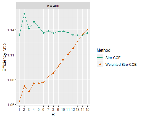
For this purpose, we chose samples of sizes $n\in\{128,256,512,1024,2048,4096\}$ in order to carry out the performance analysis based on the procedure described below. Each dataset has been split into $16$ equal subsets. Then, for each $R\in\{1,\dots,15\}$, the first $R$ part was used as batch, while the remaining ones made up the streaming phase. Results of this extended set of simulations are reported in Table 6.1, as well as graphically in Figure 6.1 where both methods are compared in terms of efficiency.

$R$	$\varrho$	$\varrho_{W}$
1	1,9284	1,4344
2	1,9494	1,4646
3	1,9976	1,5129
4	1,8993	1,4770
5	1,8980	1,4992
6	1,8561	1,4998
7	1,8793	1,5394
8	1,8812	1,5699
9	1,8595	1,5916
10	1,8623	1,6308
11	1,8289	1,6476
12	1,7934	1,6625
13	1,7278	1,6426
14	1,8244	1,7564
15	1,7607	1,7333

(a) $n=128$, $\mathrm{RMSE}=1,0407$

$R$	$\varrho$	$\varrho_{W}$
1	1,1757	1,1624
2	1,1426	1,0998
3	1,1367	1,0889
4	1,1430	1,1040
5	1,1341	1,0841
6	1,1402	1,0933
7	1,1445	1,1028
8	1,1462	1,1082
9	1,1434	1,1070
10	1,1341	1,0962
11	1,1325	1,0972
12	1,1324	1,1015
13	1,1331	1,1092
14	1,1360	1,1099
15	1,1167	1,0903

(b) $n=256$, $\mathrm{RMSE}=1,0062$

$R$	$\varrho$	$\varrho_{W}$
1	1,2574	1,0344
2	1,2264	1,0387
3	1,2212	1,0540
4	1,2231	1,0410
5	1,2234	1,0368
6	1,2255	1,0272
7	1,2255	1,0224
8	1,2259	1,0168
9	1,2282	1,0108
10	1,2279	1,0092
11	1,2281	1,0106
12	1,2297	1,0194
13	1,2302	1,0405
14	1,2321	1,0840
15	1,2355	1,1504

(c) $n=512$, $\mathrm{RMSE}=0,9485$

$R$	$\varrho$	$\varrho_{W}$
1	1,3942	1,0431
2	1,3462	1,0167
3	1,3036	1,0066
4	1,3089	1,0056
5	1,2886	1,0032
6	1,2730	1,0020
7	1,2788	1,0017
8	1,2816	1,0017
9	1,2795	1,0025
10	1,2628	1,0049
11	1,2521	1,0098
12	1,2557	1,0185
13	1,2402	1,0337
14	1,2373	1,0604
15	1,2542	1,1163

(d) $n=1024$, $\mathrm{RMSE}=1,0306$

$R$	$\varrho$	$\varrho_{W}$
1	1,2827	1,0110
2	1,2833	1,0110
3	1,2833	1,0110
4	1,2808	1,0112
5	1,2792	1,0117
6	1,2811	1,0126
7	1,2788	1,0137
8	1,2718	1,0150
9	1,2715	1,0168
10	1,2774	1,0192
11	1,2780	1,0226
12	1,2886	1,0275
13	1,3347	1,0351
14	1,3802	1,0471
15	1,3084	1,0655

(e) $n=2048$, $\mathrm{RMSE}=0,9962$

$R$	$\varrho$	$\varrho_{W}$
1	2,7767	1,0186
2	2,7373	1,0188
3	2,7767	1,0197
4	2,7766	1,0205
5	2,7766	1,0218
6	2,7765	1,0220
7	2,7764	1,0225
8	2,7729	1,0239
9	2,7711	1,0253
10	2,7715	1,0280
11	2,7690	1,0334
12	2,7690	1,0454
13	2,7683	1,0753
14	2,7661	1,1585
15	2,7731	1,4466

(f) $n=4096$, $\mathrm{RMSE}=0,9992$

Table 6.1. Comparison of efficiencies associated with the standard Stre-GCE and the weighted Stre-GCE methods. The efficiency ratios (5.2) for standard Stre-GCE and (6.6) for Weighted Stre-GCE are shown at datasets of sizes $n\in\{128,256,512,1024,2048,4096\}$. Each dataset was divided in $16$ parts with equal cardinality: for each $R\in\{1,\dots,15\}$, an associated simulation test was run using the first $r$ parts as batch and the remaining $16-R$ parts for the streaming phase.

Figure 6.1. Performance of standard Stre-GCE and Weighted Stre-GCE methods in terms of efficiencies ratios (5.2) and (6.6).

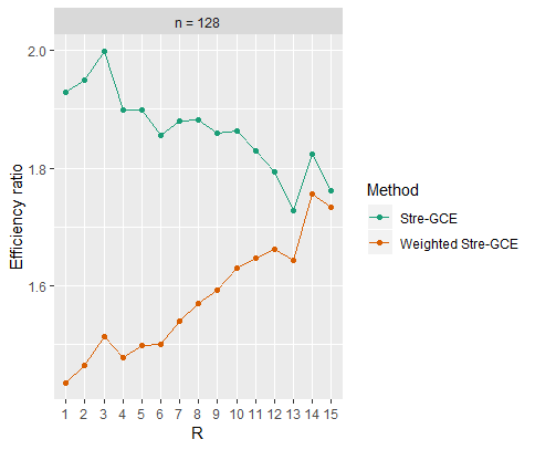
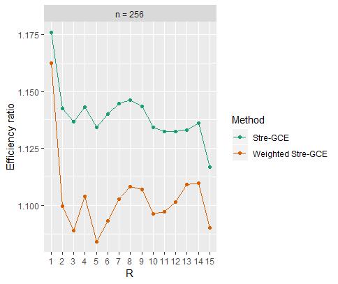
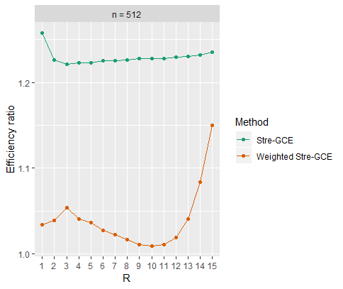
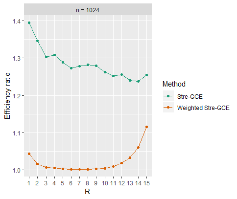
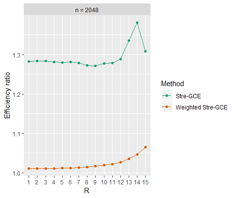
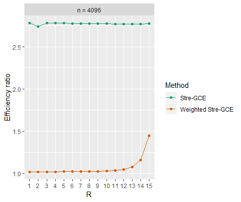
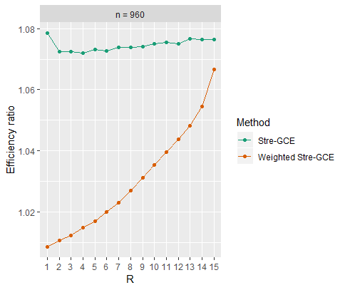
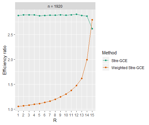
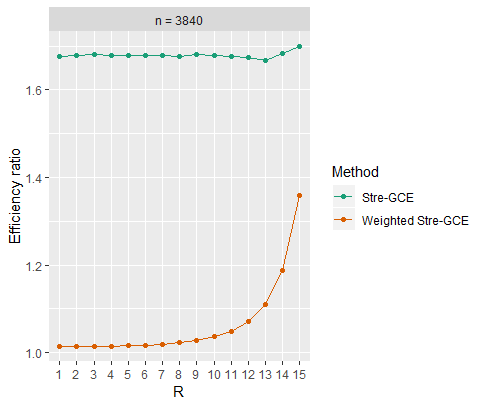
The same analysis described above has been carried out on datasets of sizes $n\in\{480,960,1920,3840\}$ already considered in Table 5.1, in order to explore the change in the performance when moving from standard Stre-GCE to Weighted Stre-GCE. The results are presented in Figure 6.2.

Figure 6.2. Performance of standard Stre-GCE and Weighted Stre-GCE methods in terms of efficiencies ratios (5.2) and (6.6).

7. Discussion

We summarise some of the features that can be extracted from the previous observations and the set of simulations.

As already remarked, the order of observations for updates of cross entropy is irrelevant when the update involves all the data at the same time (standard GCE), whereas Stre-GCE gives relevance to the temporal structure, i.e. the timeflow represented by the data stream. This additional structure allows to distinguish between two sources of entropy and is linked to the relaxation of consistency constraints (as remarked in Section 3). On the other hand, results are not compromised by multicollinearity in contrast to other recursive approaches, as can be expected from the broad scope of applicability of entropy-based methods.

The timeflow of data also raises other concerns: for instance, standardization assumes the knowledge of the full dataset, therefore it can be applied only to the available data in a streaming context. Alternatively, the performance of the Stre-GCE method on the full standardized dataset can only be used a posteriori, which is the approach we adopted to get the results shown in Table 5.1. It is worth remarking that the simulation we carried out with standardized variables shows a reduced dependence on the batch size: the differences among RMSEs at different batch sizes are often smaller than the last significant digit shown in Table 5.1.

We have considered a “hybrid” approach through blocks, in order to interpolate between Stre-GCE ($g=1$) and standard GME ($g=n$). Indeed, the relationship between GME and Stre-GCE can be seen as a specific application of the MEP methods at different time scales. In physical terms, the assumption (2.3) of variables being replaced by their associated first moments, is valid under certain conditions, often including the characteristic time scales of the model (e.g., thermalization time). Hence, blocks at $g\notin\{1,n\}$ represent a new approach to deal with the notion of metastability also discussed in a different framework in [34, 35]. We stress that, in applications, streaming blocks are not only an additional tool to refine the algorithm, but can characterize specific models where data clusters add in a sequential way.

We note that Stre-GCE is more sensitive to the dataset than standard GCE with uniform prior: this sensitivity does not only rely on the data, but also on their ordering within the stream. Different factors may result in the distortion of the estimates, ranging from the consolidation of fluctuations during the streaming phase, to excessive importance linked to streaming data. In order to avoid data overrating during the streaming phase, yet preserving the temporal structure, an alternative streaming algorithm has been proposed (i.e. Weighted Stre-GCE, see Section 6). Specifically, the balancing of the relaxation of consistency constraints with the inclusion of new observation has led to the introduction of weights (6.2). These weights are natural in that they can be described as a recursive relationship linking the objective function at the $i^{\text{th}}$ step to that at the $(i+1)^{\text{th}}$ step independently on the dataset. The quality of the estimates is consistently improved when compared with the simple Stre-GCE method, as it can be seen in the comparison Table 6.1. In particular, the deviations from a monotone behaviour of the RMSE as the data dimension increases are mitigated in the Weighted Stre-GCE approach and results are consistent with those for standard GCE: in this regard, weights act as a “smoothing” factor.

When the batch dimension is large, the standard Stre-GCE and Weighted Stre-GCE methods tend to produce similar results. Furthermore, it is noted that a short streaming phase in the Weighted Stre-GCE approach gives more relevance to the individual data during the stream, so they may affect the performance of the method. In fact, for each fixed dataset, the larger the streaming, the smaller the batch and the RMSE associated with Weighted Stre-GCE tends to increase along with the size of the batch (also see Figures 6.1 and 6.2). New data can suppress fluctuations, resulting into a tendency to perform better on larger datasets, area in which both GME and GCE struggle the most from a computational point of view.

One way to improve the results and avoid the decline in performance is to enter a control step in the Stre-GCE algorithm, that is, the choice of whether or not to update the distribution. If we fix a performance indicator $\Delta(\boldsymbol{\hat{\beta}})$ for the estimate $\boldsymbol{\hat{\beta}}$, at the $(i+1)^{\text{th}}$ iteration step we can choose between either the last available estimate $\boldsymbol{\hat{\beta}}_{i}$ or the new potential estimate $\boldsymbol{\hat{\beta}}_{i+1}^{(\text{new)}}$ obtained from the update rules (LABEL:eq:_update_step,_estimates) or (6.2). The choice is based on the following criterion

$$\Delta(\boldsymbol{\hat{\beta}}_{i+1})=\min\left\{\Delta(\boldsymbol{\hat{\beta}}_{i}),\Delta(\boldsymbol{\hat{\beta}}_{i+1}^{(\text{new)}})\right\}.$$ (7.1)

which only relies on the data available at the $(i+1)^{\text{th}}$ step. However, in this work we focused on the RMSE as performance indicator for a posteriori evaluation, always involving the whole dataset. Another quantity of interest is represented by entropy production, which is related to nonequilibrium processes. In particular, we can consider the evolution for the model itself, which may vary during the data stream. For instance, the parameters $\boldsymbol{\beta}$ may change, or nonlinearities could appear outside a given time scale. In these cases, one cannot rely on the approximate estimate provided by GCE applied on the batch only, as new data may contain relevant information on the parameters and their evolution. We will consider these approaches in a separate paper.

Finally, we remark that Stre-GCE assigns asymmetric roles to signal and error in an intrinsic way, namely, without the introduction of any additional parameter to be estimated. The Weighted Stre-GCE presented in this work is in line with such a characteristic: the weights $w_{\beta}^{(i)},w_{\varepsilon}^{(i)}$ in (6.1) are derived solely from the definition of cardinality of sets and from the different contributions attributed to the signal and the error during the updates. A similar approach has been formalized also in the context of statistical physics using algebraic methods [34].

8. Conclusion and future perspectives

This work aimed at introducing the Stre-GCE method to combine an adaptive approach with generalized entropy methods. The qualitative discussion and the quantitative analysis that have been performed suggest several extensions and applications for future investigations, some of which have already been mentioned.

Following the observations in Section 7, the algorithm can be improved choosing between the update or the preservation of the actual distribution $\mathbf{P}^{\beta}$ at each step. In this regards, either the Root-Mean-Square Error or the entropy production represent criteria that might drive the decision process. Additionally, we remark that the comparison between Stre-GCE and standard GCE can be used a posteriori to provide a finer description of blocks of data in the flow of time in terms of the quality of the estimates.

We can consider more general forms of recursive weights between the contributions of signal and error, that is a sequence $\gamma_{i}\in[0,1]$, $i\in\{1,\dots,n\}$, a deformation of the objective function (4.5) defined by $\gamma_{i+1}\cdot\mathrm{D_{KL}}(\mathbf{P}^{\beta}||\mathbf{\hat{P}}_{i}^{\beta})+(1-\gamma_{i+1})\cdot\mathrm{D_{KL}}(\mathbf{p}_{i+1}^{\varepsilon}||\mathbf{u}_{i}^{\varepsilon})$ and a given rule $\gamma_{i+1}=f_{i}(\gamma_{i})$. Depending on the choices of $f_{i}$, one can describe different balancing modes between prior information and new data. With respect to this, the dependence of the performance of the weighted algorithm in terms of initial weights and update rule should be investigated too.

The streaming approach is best suited to models that show a strong temporal component. Therefore, it seems natural to adapt the Stre-GCE algorithm and its generalizations to time-varying models, e.g. considering a time-varying parameter $\beta$ in the relation (2.1). This framework also suggests to further explore the complementary aspects of both the batch and the streaming phases as the information extraction from data goes on: in fact, they may alternate during the time window under consideration. This situation may be analyzed using a well-known approach to explore time asymmetry, namely, non-commutativity of two learning modes, that is, the batch learning mode and the streaming learning mode.

Finally, applications to real systems will be considered in next investigations. The learning aspects, also including recursive weights, and the entropy production could be used in both dynamical frameworks such as those observed in the psychological sciences (e.g. the psychotherapeutic process that aims at change and is expected to evolve over time) and in the context of reasoning under uncertainty of knowledge-based social networks: both of them provide natural settings where the sequential data acquisition, the evolution over time, the combination of prior and new information, as well as their quantification play a fundamental role.

References

- [1] R. J. Solomonoff, A formal theory of inductive inference, Parts i, ii, Inform. control 7 (1, 2) (1964) 1–22, 224–254. doi:10.1016/s0019-9958(64)90131-7.
- [2] A. Holzinger, M. Hörtenhuber, C. Mayer, M. Bachler, S. Wassertheurer, A. J. Pinho, D. Koslicki, On Entropy-Based Data Mining, in: Interactive Knowledge Discovery and Data Mining in Biomedical Informatics, Springer Nature, 2014, pp. 209–226. doi:10.1007/978-3-662-43968-5_12.
- [3] A. L. Berger, V. J. Della Pietra, S. Della Pietra, A maximum entropy approach to natural language processing, Comput. Linguist. 22 (1) (1996) 39–71.
- [4] G. Gladyshev, Thermodynamic Theory of the Evolution of Living Beings, Nova Science Pub. Inc., 1997.
- [5] A. Golan, G. Judge, D. Miller, Maximum entropy econometrics: Robust estimation with limited data, Chichester, UK: John Wiley & Sons, 1996.
- [6] A. Golan, Information and Entropy Econometrics – A Review and Synthesis, Found. Trends Econom. 2 (1-2) (2007) 1–145. doi:10.1561/0800000004.
- [7] A. Golan, Foundations of Info-Metrics: Modeling, Inference, and Imperfect Information, New York, NY: Oxford University Press, 2018. doi:10.1093/oso/9780199349524.001.0001.
- [8] E. Ciavolino, J. J. Dahlgaard, Simultaneous equation model based on the generalized maximum entropy for studying the effect of management factors on enterprise performance, J. Appl. Stat. 36 (7) (2009) 801–815. doi:10.1080/02664760802510026.
- [9] E. Ciavolino, A. D. Al-Nasser, Comparing generalised maximum entropy and partial least squares methods for structural equation models, J. Nonparametr. Stat. 21 (8) (2009) 1017–1036. doi:10.1080/10485250903009037.
- [10] E. Ciavolino, A. Calcagnì, Generalized cross entropy method for analysing the SERVQUAL model, J. Appl. Stat. 42 (3) (2014) 520–534. doi:10.1080/02664763.2014.963526.
- [11] E. Ciavolino, M. Carpita, The GME estimator for the regression model with a composite indicator as explanatory variable, Qual. Quant. 49 (3) (2014) 955–965. doi:10.1007/s11135-014-0061-4.
- [12] L. Amusa, T. Zewotir, D. North, Examination of entropy balancing technique for estimating some standard measures of treatment effects: a simulation study, Electron. J. Appl. Stat. Anal. 12 (2) (2019) 491–507. doi:10.1285/i20705948v12n2p491.
- [13] R. Bernardini Papalia, E. Ciavolino, GME estimation of spatial structural equations models, J. Classif. 28 (1) (2011) 126–141. doi:10.1007/s00357-011-9073-0.
- [14] E. Ciavolino, M. Carpita, A. D. Al-Nasser, Modelling the quality of work in the italian social co-operatives combining NPCA-RSM and SEM-GME approaches, J. Appl. Stat. 42 (1) (2014) 161–179. doi:10.1080/02664763.2014.938226.
- [15] E. Ciavolino, A. Calcagnì, A generalized maximum entropy (GME) estimation approach to fuzzy regression model, Appl. Soft Comput. 38 (2016) 51–63. doi:10.1016/j.asoc.2015.08.061.
- [16] D. Simon, Optimal State Estimation, Hoboken, NJ: John Wiley & Sons, 2006. doi:10.1002/0470045345.
- [17] B. Widrow, R. Winter, Neural nets for adaptive filtering and adaptive pattern recognition, Computer 21 (3) (1988) 25–39. doi:10.1109/2.29.
- [18] X. Xu, H. He, D. Hu, Efficient Reinforcement Learning Using Recursive Least-Squares Methods, J. Artif. Intell. Res. 16 (2002) 259–292. doi:10.1613/jair.946.
- [19] R. Zanetti, Recursive Update Filtering for Nonlinear Estimation, IEEE T. Automat. Contr. 57 (6) (2012) 1481–1490. doi:10.1109/tac.2011.2178334.
- [20] F. Daum, Nonlinear filters: beyond the Kalman filter, IEEE Aero. El. Sys. Mag. 20 (8) (2005) 57–69. doi:10.1109/maes.2005.1499276.
- [21] H. Bagya Lakshmi, M. Gallo, R. M. Srinivasan, Comparison of regression models under multi-collinearity, Electron. J. Appl. Stat. Anal. 11 (1) (2018) 340–368. doi:10.1285/i20705948v11n1p340.
- [22] L. D. Landau, E. M. Lifschitz, Statistical Physics, Vol. 5 of Course of Theoretical Physics, Oxford, UK: Butterworth-Heinemann, 1980.
- [23] R. P. Feynman, Statistical Mechanics: A Set Of Lectures, Advanced Books Classics (revised edition), Boulder, CO: Westview Press, 1998.
- [24] T. M. Cover, J. A. Thomas, Elements of Information Theory, Hoboken, NJ: John Wiley & Sons, 2006. doi:10.1002/047174882x.
- [25] A. I. Khinchin, Mathematical Foundations of Information Theory, Dover, 1957.
- [26] R. Dewar, Maximum Entropy Production as an Inference Algorithm that Translates Physical Assumptions into Macroscopic Predictions: Don’t Shoot the Messenger, Entropy 11 (4) (2009) 931–944. doi:10.3390/e11040931.
- [27] E. T. Jaynes, Probability Theory - The Logic of Science, Cambridge, UK: Cambridge University Press, 2003. doi:10.1017/CBO9780511790423.
- [28] A. Golan, “Maximum entropy, likelihood and uncertainty”, in: G. Erickson, J. T. Rychert, C. R. Smith (Eds.), Maximum Entropy and Bayesian Methods. Boise, Idaho, USA, 1997: Proceedings of the 17th International Workshop on Maximum Entropy and Bayesian Methods of Statistical Analysis, Vol. 98 of Fundamental Theories of Physics, Netherlands: Springer, 1998. doi:10.1007/978-94-011-5028-6.
- [29] D. P. Bertsekas, Combined primal-dual and penalty methods for constrained minimization, SIAM J. Control 13 (3) (1975) 521–544. doi:10.1137/0313030.
- [30] X. Wu, A Weighted Generalized Maximum Entropy Estimator with a Data-driven Weight, Entropy 11 (4) (2009) 917–930. doi:10.3390/e11040917.
- [31] C. Jarzynski, Nonequilibrium Equality for Free Energy Differences, Phys. Rev. Lett. 78 (14) (1997) 2690–2693. doi:10.1103/physrevlett.78.2690.
- [32] G. E. Crooks, Entropy production fluctuation theorem and the nonequilibrium work relation for free energy differences, Phys. Rev. E 60 (3) (1999) 2721–2726. doi:10.1103/physreve.60.27.
- [33] F. Pukelsheim, The Three Sigma Rule, Am. Stat. 48 (2) (1994) 88–91. doi:10.2307/2684253.
- [34] M. Angelelli, Tropical limit and micro-macro correspondence in statistical physics, J. Phys. A: Math. Theor. 50 (2017) 415202. doi:10.1088/1751-8121/aa863b.
- [35] M. Angelelli, B. Konopelchenko, Zeros and amoebas of partition functions, Rev. Math. Phys. 30 (09) (2018) 1850015. doi:10.1142/s0129055x18500150.