Group induced graphical lasso allows for discovery of molecular pathways-pathways interactions

Abstract

Complex systems may contain heterogeneous types of variables that interact in a multi-level and multi-scale manner. In this context, high-level layers may considered as groups of variables interacting in lower-level layers. This is particularly true in biology, where, for example, genes are grouped in pathways and two types of interactions are present: pathway-pathway interactions and gene-gene interactions. However, from data it is only possible to measure the expression of genes while it is impossible to directly measure the activity of pathways. Nevertheless, the knowledge on the inter-dependence between the groups and the variables allows for a multi-layer network inference, on both observed variables and groups, even if no direct information on the latter is present in the data (hence groups are considered as latent). In this paper, we propose an extension of the latent graphical lasso method that leverages on the knowledge of the inter-links between the hidden (groups) and observed layers. The method exploits the knowledge of group structure that influence the behaviour of observed variables to retrieve a two layers network. Its efficacy was tested on synthetic data to check its ability in retrieving the network structure compared to the ground truth. We present a case study on Neuroblastoma, which shows how our multi-level inference is relevant in real contexts to infer biologically meaningful connections.

1 Scientific background

The study of complex systems is typically performed through mathematical abstractions (graphs) that model the entities of the system as nodes and connections as edges. A graph is a pair $\mathcal{G}=(\mathcal{E},\mathcal{V})$ where $\mathcal{V}=\{1,\dots,d\}$ is the set of $d$ nodes and $\mathcal{E}\subseteq\mathcal{V}\times\mathcal{V}$ is the set of edges. In what follows we consider undirected graphs, for which there is no distinction between $(i,j)\in\mathcal{E}$ and $(j,i)$.
In many applications the underlying graph is not known a priori but it has to be inferred from real world observations. Gaussian graphical models (GGMs) are a popular set of methods which aim to solve the network inference problem [11]. Such models assume variables to be jointly distributed according to a zero-mean multivariate Gaussian distribution $\mathcal{N}(0,\Sigma)$ (the zero-mean assumption lets $\Sigma$ completely describe the system, without loss of generality). While a direct estimation of the covariance $\Sigma$ is possible, such matrix represents the marginal distribution of the variables, hence encoding both direct and indirect dependencies. A different approach is to estimate its inverse $\Theta=\Sigma^{-1}$ that encodes the conditional dependencies between variables, i.e., $\Theta_{ij}=0$ means that variables $i$ and $j$ are conditionally independent given all the other variables in the graph. Hence $\Theta$ can be considered as the weighted adjacency matrix of the graph $\mathcal{G}$.
A way to infer such network is through optimization of penalized maximum likelihood [7] $\operatorname{logdet}(\Theta)-\operatorname{tr}(S\Theta)~{}-~{}\alpha\|\Theta\|_{od,1}$ where $S=\frac{1}{n}X^{\top}X$ and $\|\cdot\|_{od,1}$ is the off-diagonal $\ell_{1}$ norm that enforces sparsity in the precision matrix. Indeed, a prior on the problem is the assumption that variables interact only with few others. Sparsity in the graph helps with the identifiability of the graph in the case when the number of samples is much lower than the number of variables, improves interpretability of the results and reduces noise.

Such model does not consider that real world systems are often composed by heterogeneous entities or some high-level mechanisms that group the entities in a structured manner [5]. Indeed, considering such influence during the network inference may direct the analysis towards a robust estimation of the graph.

Notation

In what follows, we will denote matrices with capital letters, such as $A$. We denote a square block of $A$ as $A_{B}$, meaning that $A$ is restricted to the rows and columns corresponding to indices in the set $B$. Similarly, we denote a non-square block as $A_{BC}$, considering rows in the set $B$ and columns in the set $C$. $A_{ij}$ indicates the entry of $A$ corresponding to the $i$-th row and $j$-th column.

2 Group induced graphical lasso

We want to infer a two-layers networks in which one layer model connections between observed variables and the other the connections between groups of these observed variables. Note that the activity of the groups cannot be directly measured and it is, therefore, latent. Nevertheless, we assume that the membership of each observed variable to one or more groups is known a priori. The goal of a advanced analysis is to provide a more complete overview of the system even though we do not expect the connections between groups to exhaustively explain the connections between observed variables. Hence we allow connections between variables that belong to different groups. To this aim we extend a state-of-the-art method for latent graphical inference (LGL) [4, 21] that takes into account the influence of latent factors without any assumption on their identities. The proposed method is Group Induced Graphical Lasso (GIGL) that considers structured regularisation over the network links to consider the group memberships of the variables.

2.1 The model

Consider $N$ observations in $O$ variables represented as a matrix $X\in\mathbb{R}^{N\times O}$ drawn from a multivariate Gaussian distribution $\mathcal{N}(0,\tilde{\Sigma}_{O})$. Observed variables $O$ describe the available samples, but their interaction is perturbed by the influence of higher-level interactions of $H$ groups which activity is unobserved (hidden). The matrix perturbation is $\tilde{\Sigma}_{O}=\Sigma_{O}-\Sigma_{OH}\Sigma_{H}^{-1}\Sigma_{OH}^{\top}$ where $\Sigma_{O}$ is the true underlying covariance of the observed variables. We aim at inferring the global precision matrix of the system given the observations $X$ and the memberships of the $O$ variables in $H$ groups. These memberships are encoded into a binary matrix $G\in\{0,1\}^{o\times h}$ where $G_{oh}=1$ if the observed variable $o$ belongs to the group $h$ and $0$ otherwise. Note that groups can overlap. Our goal is to estimate the precision matrix $\Theta$ of the following form:

$$\Theta=\Sigma^{-1}=\left[\begin{array}[]{c|ccc}&&&\\[-6.00006pt] \Theta_{H}&&\Theta_{OH}^{\top}&\\[5.0pt] \hline\cr&&&\\ \Theta_{OH}&&\Theta_{O}&\\ &&&\\ \end{array}\right].$$

where $\Theta_{H}$ and $\Theta_{O}$ represent the precision matrices between groups and variables respectively and $\Theta_{OH}$ is a possibly non-squared matrix. Note that a non-zero entry in the precision matrix $\Theta_{OH}$ should be found in correspondence of non-zero entries of $G$. Moreover, the model does not prevent the inference new connections between variables and groups, since there may be some dependency which is not known a priori.

The inference problems translates into the optimisation of a non-convex function $\mathcal{F}(\Theta,\widetilde{S}_{0},G)$

$$\begin{split}\underset{\begin{subarray}{c}\Theta\in\mathbb{R}^{(O+H)\times(O+H)}\\ \Theta\succ 0\end{subarray}}{\operatorname*{minimize}}&~{}~{}\mathcal{F}(\Theta,\tilde{(}S)_{0},G)\\ =\underset{\begin{subarray}{c}\Theta\in\mathbb{R}^{(O+H)\times(O+H)}\\ \Theta\succ 0\end{subarray}}{\operatorname*{minimize}}&-\operatorname{logdet}(\Theta)+\operatorname{tr}(S\Theta)+\lambda\|\Theta_{O}\|_{1,od}++\eta\|\Theta_{H}\|_{1,od}+\mu\bar{G}\|\Theta_{OH}\|_{1}\end{split}$$ (1)

where $S\in\mathbb{R}^{O+H}$, $S_{O}=\frac{1}{N}X^{\top}X$ and $\bar{G}=1-G$.

Problem (1) depends on three hyper-parameters $\lambda$, $\eta$ and $\mu$, which regulate the sparsity of the blocks of the matrix $\Theta$. The sparsity on the block $\Theta_{OH}$ is also enriched by the structured regularisation given by $\bar{G}$. Appendix A includes the optimisation algorithm and related mathematical derivations.

3 Experiments

We tested the effectiveness of GIGL on both synthetic and real data. Synthetic experiments show its ability in retrieving the network structure. Results on real data show how GIGL, through the imposition of prior knowledge, allows some latent patterns to emerge. We performed a model selection procedure to choose the best hyper-parameters $\lambda$, $\mu$ and $\eta$ based on the data at hand. The procedure was performed on a refined grid using the average log-likelihood score of the model with respect to test data on a 3-fold cross validation. The log-likelihood is computed as:

$$\operatorname{logdet}(\Theta_{obs})-\operatorname{tr}(\tilde{S}_{ts}\Theta_{obs}),$$ (2)

where $S_{ts}$ is the empirical covariance matrix of the test data and $\Theta_{obs}=\Theta_{O}-\Theta_{OH}\Theta_{H}^{-1}\Theta_{OH}^{\top}$.

Synthetic experiments

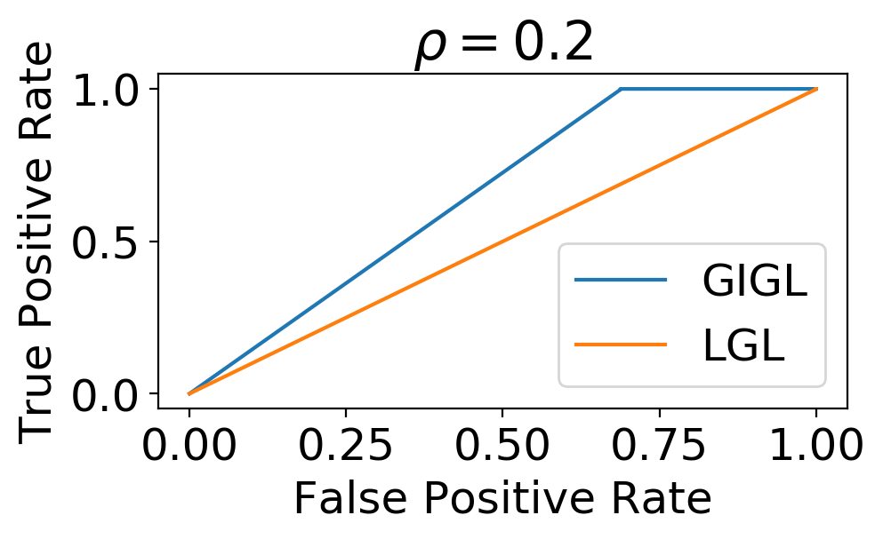
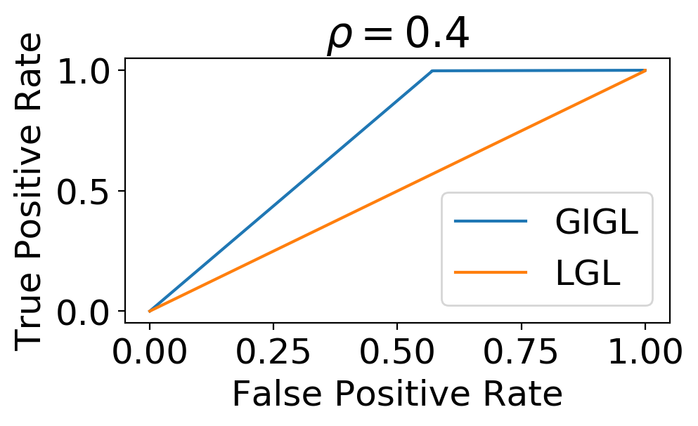
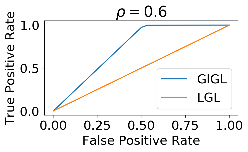
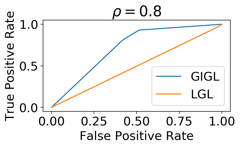
We generated four different data sets with increasing sparsity $\rho$ of the connections, with $\rho\in\{0.2,0.4,0.6,0.8\}$. Each data set has 100 latent variables and 200 observed variables. The blocks of $\Theta$ are generated such that both the global matrix and the difference $\tilde{\Theta}=\Theta_{O}-\Theta_{OH}\Theta_{H}^{-1}\Theta_{OH}^{\top}$ are positive definite. We drew 500 samples from a multivariate Gaussian distribution $\mathcal{N}(0,\tilde{\Theta}^{-1})$ to estimate the empirical covariance matrix, which is the input of GIGL. Also, we supplied to GIGL the mask for the non-zero positions of $\Theta_{OH}$. The performance of GIGL and LGL were evaluated in terms of structure recovery, based on the Receiving Operating Characteristic (ROC) curve and Area Under the Curve (AUC) (Figure 1). Note that the ROC curve requires probabilities/confidence interval to be computed. To assess the robustness of the results we estimated a confidence interval by repeating the experiments 10 times. We then computed the average of all binarised resulting matrices $\Theta_{i}$ for $i=1,\dots 10$. We interpret the average matrix $\bar{\Theta}$ as the probability of each edge to exist.

$AUC_{\rho=0.2}=0.66$

$AUC_{\rho=0.4}=0.71$

$AUC_{\rho=0.6}=0.74$

$AUC_{\rho=0.8}=0.72$

Figure 1: ROC curves of GIGL and LGL methods. The experiments were performed with an increasing sparsity of the ground truth network. The AUC of GIGL increases as the sparsity increases, while for LGL it remains stable at $0.5$ denoting that LGL tends to be less sparse than GIGL.

Neuroblastoma: a case study

We applied our method on a TCGA neuroblastoma RNA-Seq dataset. For computational ease, we considered a subset of genes known in literature to be involved in Neuroblastoma disease based on Phenopedia [20]. The resulting list of 203 genes was provided to Webgestalt [18] for a functional characterisation through a gene enrichment analysis. We ended up considereing 116 KEGG (Kyoto Encyclopedia of Genes and Genomes) [10] pathways where the subset of genes was found enriched.
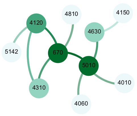
We then applied GIGL and LGL to this data by imputing the empirical covariance matrix of the gene expression and the membership of each gene to one or more pathways. Given the non-convexity of our model we optimise the model 20 times with different initialisations, which may lead to different solutions. Finally, we retain the links present at least 70% of the 20 times. Figure 3 shows the pathways-pathways interactions. The gene networks for both GIGL and LGL are included in Appendix B, due to space constraints.

Figure 2: KEGG pathways connections on Neuroblastoma estimated by GIGL. The darker colour of the node denotes its degree while the darker colour of the edge denotes the probability of its existence.

No.	Description
4060	Cytokine cytokine receptor interaction
5010	Alzheimer’s disease
670	One carbon pool by folate
4630	jak STAT signaling pathway
4120	Ubiquitin mediated proteolysis
5142	Chagas disease american trypanosomiasis
4010	MAPK signaling pathway
4150	mTor signaling pathway
4310	wnt signaling pathway
4810	Regulation of actin cytoskeleton

Figure 3: KEGG pathways description of the network nodes in Figure 3

4 Discussion

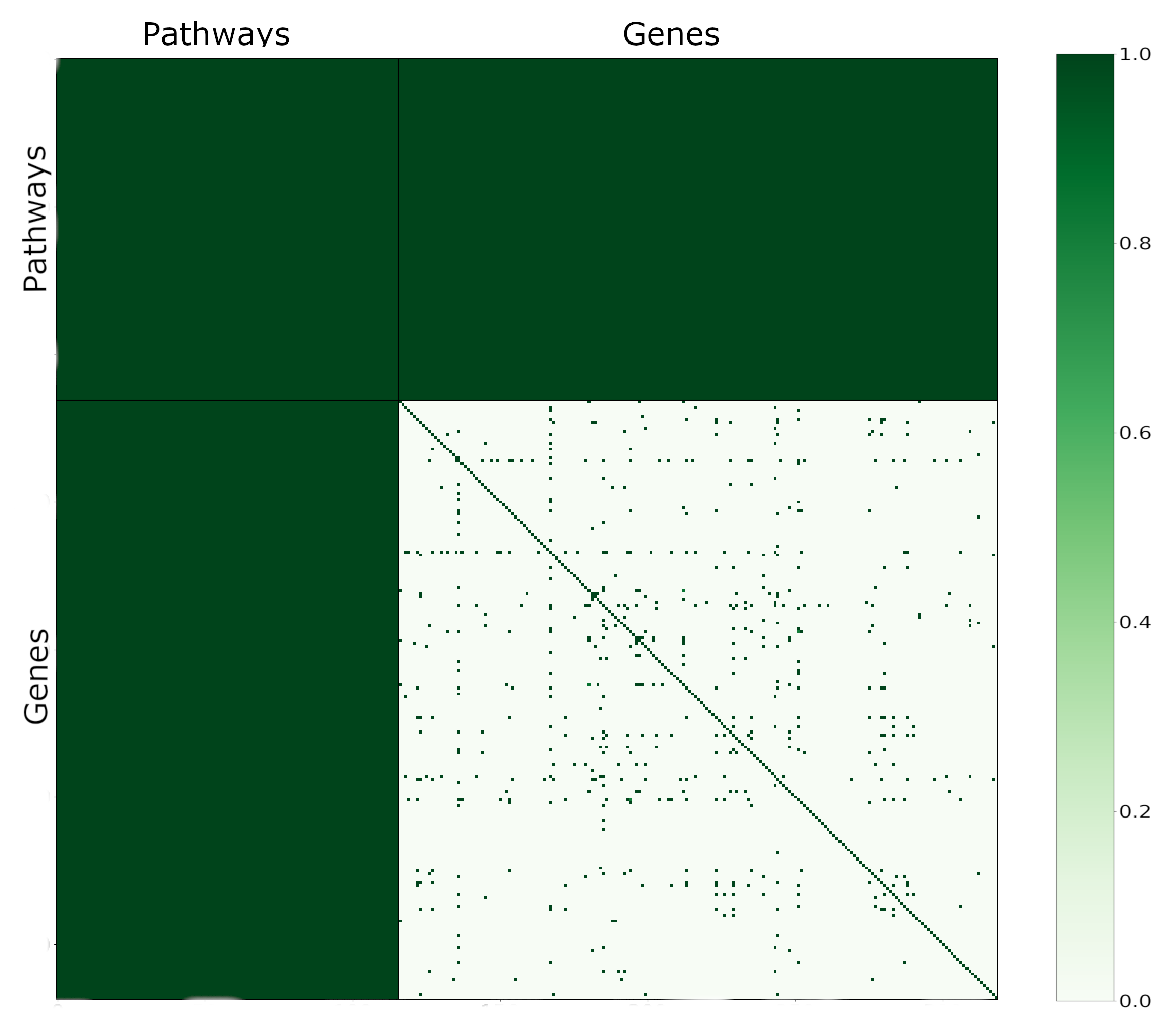
Synthetic experiments show that our method is able to correctly identify the links between latent variables acting in the system also with an increasing sparsity. As shown in Figure 1, LGL always finds dense blocks in the latent variables, while GIGL better identify the links. We also note how an increase in sparsity results in a more accurate identification of missing edges. Considering the application on neuroblastoma, we retrieved two gene interactions network, one for both GIGL and LGL (in Appendix B Figures 5 and 6). GIGL is able to identify pathways-pathways interactions (Figure 3). 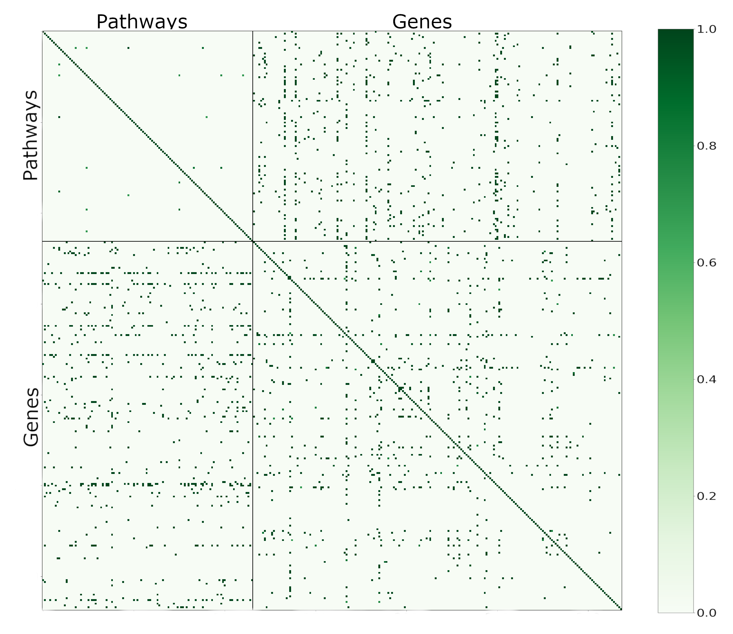The difference between the sparsity level of the networks as estimated by the two methods is also more generally visible in Figures 4(a) and 4(b). The inferred co-expression networks (Figures 5 and 6) include four common genes that emerge above others. These genes are PLEKHA4, IL6, S100B and NTRK. While the relevance of IL6 [17, 22] and NTRK [13] in neuroblastoma is a known fact, the role of the remaining two genes is still under investigation. Differently from PLEKHA4 which is poorly annotated, S100B is a well characterized gene whose chromosomal rearrangements and altered expression are known to be implicated in several neurological, neoplastic, and other types of diseases, including Alzheimer’s disease, Down’s syndrome and epilepsy. In GIGL network (Figure 5) there are more hub genes (i.e., genes highly connected) than in LGL (Figure 6). The hubs genes are: MICA, EGFR, NEFL, MYO10, VDR, HFE, HLA-C, GHR, PDLIM1, APOE, DAB2, PALU, CEBPA, IL-33. The involvement in Neuroblastoma of the first 7 genes of this list is present in literature [2, 3, 19, 1, 15, 6]. Also Figure 3 shows that “Alzheimer’s disease” and “One carbon pool by folate” are the two most strongly connected pathways. Folic acid has been recently connected to childhood cancer [14], while the one-carbon pathway was linked to Alzheimer’s [8]. Figure 3 also shows a clique between “Wnt signaling”, “Ubiquitin mediated proteolysis” and “One carbon pool by folate” pathway. It is known that WNT signaling pathway plays significant roles in the survival, proliferation, and differentiation of human neuroblastoma [16] and “Ubiquitin mediated proteolysis” is crucial in the regulated degradation of proteins involved in neuroblastoma proliferation and survival [9].
In this paper we proposed an extension of the latent graphical lasso that considers prior knowledge on the interlinks to retrieve connections between both observed and latent entities. Our method can be used to look at different network topologies that can emerge by imposing different group priors on the observed variables. The method allows for a straightforward application to real-world data, not limited to biological data sets. Indeed, while propose it for groups of variables this may also be used for general known connections between latent and observed variables that do not translate into memberships. In this work we applied our method only on a small subset of Neuroblastoma data, we aim at applying to a larger dataset and to compare the priors between different biological groups. We also plan to compare it with other methods that perform multi-layer inference [5, 12] that have different assumptions on data generation to look for evidence that emerges with more than one methodology.

Appendix A Optimization algorithm

Given problem (1), we report the mathematical steps required to reach the form of Algorithm 1. In particular the problem has $H$ latent variables that need to be estimated from input data. This purpose is reached through Expectation Maximization.

Expectation step

We compute the expected value of the penalized negative log-likelihood function given $S_{O}$ and $K^{t-1}$.

$$\begin{split}\mathcal{Q}(K|K^{t-1})&=\mathbb{E}_{X_{H}|X_{O},\Theta^{t-1}}\bigg{[}-\text{log det}(\Theta)+\text{tr}(S\Theta)+\lambda\|\Theta_{O}\|_{1,od}++\eta\|\Theta_{H}\|_{1,od}+\mu\bar{G}\|\Theta_{OH}\|_{1}\bigg{]}\\ &=-\text{log det}(\Theta)+\text{tr}\big{(}\mathbb{E}_{X_{H}|X_{O},\Theta^{t-1}}(S)\Theta\big{)}+\lambda\|\Theta_{O}\|_{1,od}++\eta\|\Theta_{H}\|_{1,od}+\mu\bar{G}\|\Theta_{OH}\|_{1}\end{split}$$ (3)

Let $\Sigma^{t}=(\Theta^{t-1})^{-1}$. Then,

$$\mathbb{E}_{X_{H}|X_{O},\Theta^{t-1}}(S_{OH})=\widetilde{S}_{OH}=S_{O}(\Sigma^{t}_{O})^{-1}\Sigma^{t}_{OH}$$ (4)

$$\mathbb{E}_{X_{H}|X_{O},\Theta^{t-1}}(S_{H})=\widetilde{S}_{H}=\Sigma^{t}_{O}-(\Sigma^{t}_{OH})^{\top}(\Sigma^{t}_{O})^{-1}\Sigma^{t}_{OH}+(\Sigma^{t}_{OH})^{\top}(\Sigma^{t}_{O})^{-1}S_{O}(\Sigma^{t}_{O})^{-1}\Sigma^{t}_{OH}$$ (5)

Maximization step

After we compute the expectation we can reconstruct the global matrix $S$ where we need to rectify $S_{O}$ by adding the influence of the hidden factors. Hence,

$$\widetilde{S}_{O}=S_{O}+\widetilde{S}_{OH}(\widetilde{S}_{H})^{-1}\widetilde{S}_{OH}^{\top}$$ (6)

ending with

$$\tilde{S}=\left[\begin{array}[]{c|ccc}&&&\\[-6.00006pt] \widetilde{S}_{H}&&\widetilde{S}_{OH}^{\top}&\\[5.0pt] \hline\cr&&&\\ \widetilde{S}_{OH}&&\widetilde{S}_{O}&\\ &&&\\ \end{array}\right].$$ (7)

The maximization step translates into a weighted graphical lasso [7] that can be easily be solved as the standard graphical lasso by using a matrix regulariser. This matrix regulariser will enforce the group structure and will allow pattern to emerge.

$$\begin{split}\Theta^{t}=\underset{\begin{subarray}{c}\Theta\in\mathbb{R}^{(O+H)\times(O+H)}\\ \Theta\succ 0\end{subarray}}{\text{minimize}}-\text{log det}(\Theta)+\text{tr}(\tilde{S}\Theta)+\lambda\|\Theta_{O}\|_{1,od}++\eta\|\Theta_{H}\|_{1,od}+\mu\bar{G}\|\Theta_{OH}\|_{1}\end{split}$$ (8)

Algorithm 1 GIGL($\tilde{S}_{O},G,\lambda,\eta,\mu)$

1:$\bar{G}=1-G$

2:for $t=1,\dots,\text{max\_iter}$ do

3:     $\Sigma^{t}=(\Theta^{t-1})^{-1}$

4:     $\widetilde{S}_{OH}=S_{O}(\Sigma^{t}_{O})^{-1}\Sigma^{t}_{OH}$

5:     $\widetilde{S}_{H}=\Sigma^{t}_{O}-(\Sigma^{t}_{OH})^{\top}(\Sigma^{t}_{O})^{-1}\Sigma^{t}_{OH}+(\Sigma^{t}_{OH})^{\top}(\Sigma^{t}_{O})^{-1}S_{O}(\Sigma^{t}_{O})^{-1}\Sigma^{t}_{OH}$

6:     $\widetilde{S}_{O}=S_{O}+\widetilde{S}_{OH}(\widetilde{S}_{H})^{-1}\widetilde{S}_{OH}^{\top}$

7:     $\tilde{S}=\left[\begin{array}[]{c|ccc}&&&\\[-6.00006pt] \widetilde{S}_{H}&&\widetilde{S}_{OH}^{\top}&\\[5.0pt] \hline\cr&&&\\ \widetilde{S}_{OH}&&\widetilde{S}_{O}&\\ &&&\\ \end{array}\right].$

8:     $R=ones(O+H,O+H)$

9:     $R=R-diag(R)$

10:     $R_{O}=\lambda*R_{O},R_{OH}=\mu*\bar{G},R_{H}=\eta*R_{H}$

11:     $\Theta^{t}=\underset{\begin{subarray}{c}\Theta\end{subarray}}{\text{minimize}}-\text{log det}(\Theta)+\text{tr}(\tilde{S}\Theta)+R\|\Theta\|_{1}$ return $\Theta$

Appendix B Retrieved Neuroblastoma networks

We applied both GIGL and LGL to Neuroblastoma data to show how our method allows to extract information on group links rather than only on gene co-expression networks. This can be seen in Figures 4(a) and 4(b). Here we show the adjacency matrices that are thresholded at 70% of occurrences of the edges. It is easy to see that LGL (Figure 4(b)) retrieves a completely dense network on the pathways interactions while GIGL (Figure 4(a)) is able to retrieve some strong connections between them.

Interestingly, the cross-validated hyper-parameter $\eta$ is so high to enforce the Pathways-Genes interaction sub-matrices to contain only the prior knowledge links. This proves that this group structure is present in the data and the model automatically recognises it using a high regularisation.

(a) GIGL adjacency matrix of neuroblastoma gene co-expression and pathways-pathways interactions network.

(b) LGL adjacency matrix of neuroblastoma gene co-expression. LGL method does not enforce sparsity in the latent sub-block of the matrices, hence the pathways-pathways interaction as well as the pathways-genes interactions are completely dense.

Figure 4: Comparison between the adjacency matrix obtained on Neuroblastoma data using GIGL and LGL model.

Figure 5: Neuroblastoma gene network estimated by GIGL. The more central and bigger nodes are the ones with highest degree.

Figure 6: Neuroblastoma gene network estimated by LGL [21]. The more central and bigger nodes are the ones with highest degree.

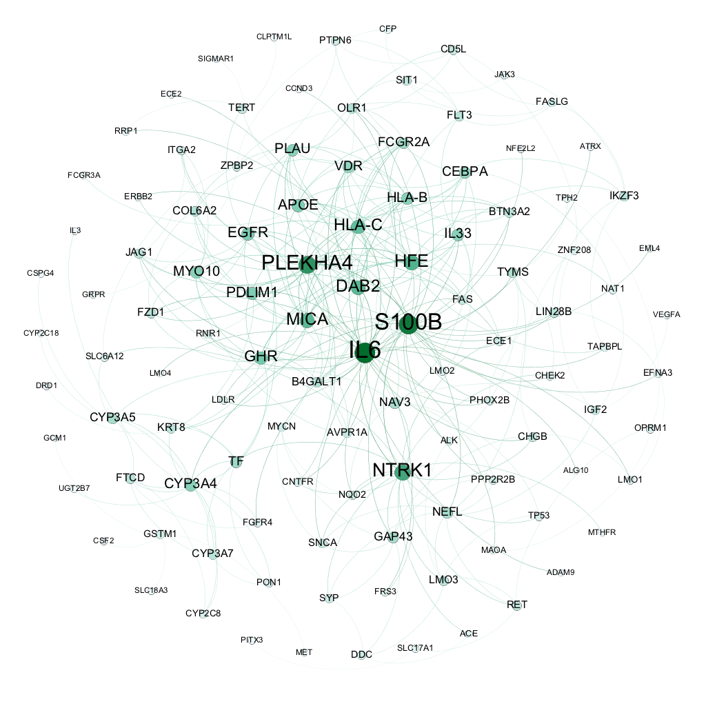
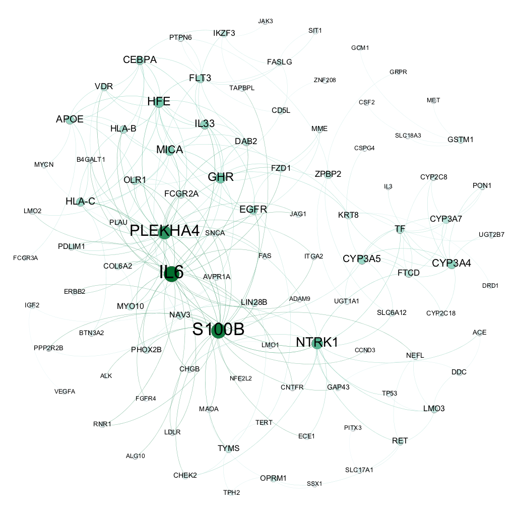
Figures 5 and 6 depict the gene co-expression networks obtained with GIGL and LGL. While there exists some shared hubs across the two networks, GIGL estimates more hubs emerging as relevant which were not found by LGL. It seems that the grouping of pathways enforces these genes to emerge. Interestingly, the majority of such genes can be found in literature to have well-known connections with Neuroblastoma.

References

- [1] Francesca Bini, Alessia Frati, Mercedes Garcia-Gil, Chiara Battistini, Maria Granado, Maria Martinesi, Marco Mainardi, Eleonora Vannini, Federico Luzzati, Matteo Caleo, et al. New signalling pathway involved in the anti-proliferative action of vitamin d3 and its analogues in human neuroblastoma cells. a role for ceramide kinase. Neuropharmacology, 63(4):524–537, 2012.
- [2] Lucia Borriello, Robert C Seeger, Shahab Asgharzadeh, and Yves A DeClerck. More than the genes, the tumor microenvironment in neuroblastoma. Cancer letters, 380(1):304–314, 2016.
- [3] Mario Capasso, Sharon J Diskin, Flora Cimmino, Giovanni Acierno, Francesca Totaro, Giuseppe Petrosino, Lucia Pezone, Maura Diamond, Lee McDaniel, Hakon Hakonarson, et al. Common genetic variants in nefl influence gene expression and neuroblastoma risk. Cancer research, pages canres–0431, 2014.
- [4] Venkat Chandrasekaran, Pablo A Parrilo, and Alan S Willsky. Latent variable graphical model selection via convex optimization. In Communication, Control, and Computing (Allerton), 2010 48th Annual Allerton Conference on, pages 1610–1613. IEEE, 2010.
- [5] Lulu Cheng, Liang Shan, and Inyoung Kim. Multilevel gaussian graphical model for multilevel networks. Journal of Statistical Planning and Inference, 190:1–14, 2017.
- [6] NC Cheng, M Beitsma, A Chan, I den Camp Op, A Westerveld, J Pronk, and R Versteeg. Lack of class i hla expression in neuroblastoma is associated with high n-myc expression and hypomethylation due to loss of the memo-1 locus. Oncogene, 13(8):1737–1744, 1996.
- [7] Jerome Friedman, Trevor Hastie, and Robert Tibshirani. Sparse inverse covariance estimation with the graphical lasso. Biostatistics, 9(3):432–441, 2008.
- [8] Andrea Fuso, Vincenzina Nicolia, Rosaria A Cavallaro, and Sigfrido Scarpa. Dna methylase and demethylase activities are modulated by one-carbon metabolism in alzheimer’s disease models. The Journal of nutritional biochemistry, 22(3):242–251, 2011.
- [9] Barbara Hämmerle, Yania Yañez, Sarai Palanca, Adela Cañete, Deborah J Burks, Victoria Castel, and Jaime Font de Mora. Targeting neuroblastoma stem cells with retinoic acid and proteasome inhibitor. PloS one, 8(10):e76761, 2013.
- [10] Minoru Kanehisa and Susumu Goto. Kegg: kyoto encyclopedia of genes and genomes. Nucleic acids research, 28(1):27–30, 2000.
- [11] Steffen L Lauritzen. Graphical models, volume 17. Clarendon Press, 1996.
- [12] Jiahe Lin, Sumanta Basu, Moulinath Banerjee, and George Michailidis. Penalized maximum likelihood estimation of multi-layered gaussian graphical models. Journal of Machine Learning Research, 17(146):1–51, 2016.
- [13] Beata S Lipska, Elżbieta Drożynska, Paola Scaruffi, Gian Paolo Tonini, Ewa Iżycka-Świeszewska, Szymon Ziętkiewicz, Anna Balcerska, Danuta Perek, Alicja Chybicka, Wojciech Biernat, et al. c. 1810c> t polymorphism of ntrk1 gene is associated with reduced survival in neuroblastoma patients. BMC cancer, 9(1):436, 2009.
- [14] Nirmalya Roy Moulik, Archana Kumar, and Suraksha Agrawal. Folic acid, one-carbon metabolism & childhood cancer. The Indian journal of medical research, 146(2):163, 2017.
- [15] Oliver D Mrowczynski, AB Madhankumar, Becky Slagle-Webb, Sang Y Lee, Brad E Zacharia, and James R Connor. Hfe genotype affects exosome phenotype in cancer. Biochimica et Biophysica Acta (BBA)-General Subjects, 1861(8):1921–1928, 2017.
- [16] Junjira Suebsoonthron, Thiranut Jaroonwitchawan, Montarop Yamabhai, and Parinya Noisa. Inhibition of wnt signaling reduces differentiation and induces sensitivity to doxorubicin in human malignant neuroblastoma sh-sy5y cells. Anti-cancer drugs, 28(5):469–479, 2017.
- [17] Francesca Totaro, Flora Cimmino, Piero Pignataro, Giovanni Acierno, Marilena De Mariano, Luca Longo, Gian Paolo Tonini, Achille Iolascon, and Mario Capasso. Impact of interleukin-6–174 g> c gene promoter polymorphism on neuroblastoma. PloS one, 8(10):e76810, 2013.
- [18] Jing Wang, Dexter Duncan, Zhiao Shi, and Bing Zhang. Web-based gene set analysis toolkit (webgestalt): update 2013. Nucleic Acids Research, 41(W1):W77–W83, 2013.
- [19] Xiqian Wang, Jing Li, Xiao Xu, Jiachun Zheng, and Qingbo Li. mir-129 inhibits tumor growth and potentiates chemosensitivity of neuroblastoma by targeting myo10. Biomedicine & Pharmacotherapy, 103:1312–1318, 2018.
- [20] W. Yu, M. Clyne, M. J. Khoury, and M. Gwinn. Phenopedia and genopedia: disease-centered and gene-centered views of the evolving knowledge of human genetic associations. Bioinformatics, 26(1):145–146, 2010.
- [21] Ming Yuan. Discussion: Latent variable graphical model selection via convex optimization. Ann. Statist., 40(4):1968–1972, 08 2012.
- [22] Qian Zhao, Mei Jin, Da-Wei Zhang, Wen Zhao, Xi-Si Wang, Zhi-Xia Yue, Chao Duan, Cheng Huang, and Xiao-Li Ma. Serum interleukin-6 level and the rs1800795 polymorphism in its gene associated with neuroblastoma risk in chinese children. Chinese medical journal, 131(9):1075, 2018.