Implementing quantum stochastic differential equations on a quantum computer

Abstract

We study how to implement quantum stochastic differential equations (QSDEs) on a quantum computer. This is illustrated by an implementation of the QSDE that couples a laser driven two-level atom to the electromagnetic field in the vacuum state on the IBMqx4 Tenerife computer [15]. We compare the resulting master equation and quantum filtering equations to existing theory. In this way we characterize the performance of the computer.

1 Introduction

In these short notes, we study a very simple problem with a solution that is universally well-known: spontaneous decay of a laser-driven two-level atom which is coupled to the electromagnetic field in the vacuum state. The techniques that we use to discretize the quantum stochastic differential equation [14] that describes the interaction between the two-level atom and the laser field are very well-known [16, 19, 17, 2, 5, 6]. The discretized model consists of a repeated unitary interaction of the two-level atom with subsequent field qubits parametrized by a discretization parameter $\lambda$. The repeated interaction model easily leads to a quantum stochastic difference equation that has the QSDE we wish to simulate as its limit as $\lambda$ goes to zero. Note that unitarity of the interaction is preserved in the discretized model, which is a very desirable feature: e.g. after time evolution probabilities will still always take values between $0$ and $1$. Furthermore, the unitarity allows us to easily map the interaction on unitary gates in a quantum computer.

The motivation for the work we present here is twofold and aimed at a future with computers with more and more reliable qubits:

1. We wish to emphasize that quantum optics might prove a very fruitful field of application for early quantum computers. It is well-known how to discretize the type of problems that arise in quantum optics and the resulting quantum stochastic difference equations are easy to implement on a quantum computer. Moreover, the field of quantum optics historically contains many interesting problems and techniques that can serve as interesting benchmark problems for early quantum computers.

2. On a quantum computer we can do a fully coherent simulation of a system in interaction with the electromagnetic field. That is, on a large enough quantum computer, we can simulate the complete unitary that describes the interaction between system and field, putting us past standard analyses using master equations or quantum filtering equations [3, 8, 9, 4] because we also have a complete description of the field to our availability. This could be very useful if we wish to simulate non-Markovian networks of systems interacting at different points with the same field, possibly containing fully coherent feedback loops [11, 10].

The remainder of these notes is organized as follows. Section 2 introduces the QSDE that we wish to simulate on a quantum computer: a laser driven two-level atom in interaction with the vacuum EM-field. We discuss repeated unitary interaction models, the resulting quantum stochastic difference equations and discuss how to take the limit to obtain quantum stochastic differential equations [19, 17, 2, 5, 6]. Next, we introduce the repeated interaction that leads to the QSDE corresponding to the problem at hand: a laser driven two-level atom in interaction with the vacuum EM-field. Section 3 describes how we have implemented the repeated interaction model of Section 2 on the IBMqx4 Tenerife quantum computer [15].

Section 4 presents the results of our simulations. We compute the reduced dynamics of the two-level atom from the simulation results and compare it to the dynamics given by the theoretical master equation, derived from the underlying discrete model. We also compute the conditional dynamics of the two-level atom conditioned on both counting photons in the field and observing a field quadrature in the field and compare the results to the quantum filtering equations derived from the underlying discrete model [7, 12, 6, 13]. Reproducing the correct quantum filtering equations would give an indication that the simulation also reproduces the correlation between the field and the two-level atom correctly.

In Section 5, we formulate some conclusions from our results. It should be noted that currently only very limited simulations can be done due to the small number of reliable qubits in the quantum computers that are currently available. In a 5 qubit machine such as the IBMqx4, we only have 4 field qubits to our availability, severely limiting our simulation capabilities. The work in these notes should be seen through the lens of a hoped-for strong increase in the computing capacity in the near future.

2 Quantum stochastic difference equations

We will now first introduce the problem that we will be studying in this paper. We consider a two-level atom with a coupling to the electromagnetic field. We will let the two-level atom be driven by a laser. We will not model the laser by an additional channel in the field that is in an coherent state, but will directly introduce the Rabi oscillations induced by the laser field as a Hamiltonian term in the QSDE. We will use the following notation throughout the paper: $\sigma_{x},\sigma_{y}$ and $\sigma_{z}$ are the standard Pauli matrices. Furthermore, $\sigma_{+}$ and $\sigma_{-}$ are the raising and lowering operator matrix of the two-level atom, respectively. The interaction of the laser driven two-level atom with the vacuum electromagnetic field is given by the following quantum stochastic differential equation (QSDE) in the sense of [14]

$$\begin{split}dU_{t}=\Big{\{}\sqrt{\kappa}\sigma_{-}dA_{t}^{*}-\sqrt{\kappa}\sigma_{+}dA_{t}-\frac{1}{2}\kappa\sigma_{+}\sigma_{-}dt-i\omega\sigma_{+}\sigma_{-}dt-i\frac{\Omega}{2}\sigma_{y}dt\Big{\}}U_{t},\ \ \ U_{0}=I,\end{split}$$ (1)

where $\kappa$ is the decay rate, $\omega$ is the transition frequency of the two-level atom and $\Omega$ is the frequency of the Rabi oscillations induced by a laser field.

In order to simulate Eqn (1) on a quantum computer, we first need to introduce the discrete models (see e.g. [6] for a detailed introduction) that in a suitable limit will converge to a quantum stochastic differential equation [19, 17, 2, 5] such as Eqn (1). To this end we first define a time interval $[0,T]$. We divide this time interval into $N$ equal sub intervals of length $T/N$. We define $\lambda:=\sqrt{T/N}$, i.e. we have $N$ sub intervals of length $\lambda^{2}$. With each sub interval we associate a two-level quantum system representing the slice of the (truncated) field that interacts with the two-level atom at that moment. In this way we obtain a repeated interaction

$$U(l)=\overleftarrow{\prod}_{i=1}^{l}M_{i}=M_{l}M_{l-1}\ldots M_{2}M_{1},\ \ \ \ 1\leq l\leq N.$$ (2)

Here $M_{i}$ is a unitary operator that couples the two-level atom and the $i$th field slice which is here also represented by a two-level system. Note that we take all $M_{i}$’s to be identical apart from the fact that they all act on their own slice of the field. Furthermore, we will let the $M_{i}$’s be a function of $\lambda$, such that if $\lambda$ goes to $0$ (i.e. $N$ goes to infinity) the $M_{i}$’s converge to the identity map $I$. That is, we will get more and more interactions, with smaller and smaller effect.

We now introduce linear operators $M^{\pm},M^{+},M^{-}$ and $M^{0}$ [6], acting on the two-level atom Hilbert space, in such a way that we have the following decomposition

$$M_{i}-I=M^{\pm}\otimes\Delta\Lambda(i)+M^{+}\otimes\Delta A^{*}(i)+M^{-}\otimes\Delta A(i)+M^{0}\otimes\Delta t(i),$$ (3)

where the discrete quantum noises (see e.g. [6]) are given by

$$\begin{split}&\Delta\Lambda(i):=(\sigma_{+}\sigma_{-})_{i},\ \ \ \ \Delta A^{*}(i):=\lambda(\sigma_{+})_{i},\\ &\Delta A(i):=\lambda(\sigma_{-})_{i},\ \ \ \ \Delta t(i):=\lambda^{2}I_{i}.\end{split}$$

Note that this decomposition uniquely defines the coefficients $M^{\pm},M^{+},M^{-}$ and $M^{0}$ and note that these coefficients are all a function of $\lambda$, which we leave implicit to keep our notation light. Furthermore, we usually omit the tensor products in Eqn (3) to keep the notation light.

We can now write Eqn (2) as the following quantum stochastic difference equation (see e.g. [6])

$$\begin{split}\Delta U(l):={}&U(l)-U(l-1)=\\ ={}&\Big{\{}M^{\pm}\Delta\Lambda(l)+M^{+}\Delta A^{*}(l)+M^{-}\Delta A(l)+M^{0}\Delta t(l)\Big{\}}U(l-1),\end{split}$$ (4)

where $1\leq l\leq N$ and $U(0)=I$. We now have the following theorem due to Parthasarathy [19] (weak convergence), Parthasarathy and Lindsay [17] (weak convergence of the quantum flow) and Attal and Pautrat [2] (strong convergence uniform on compact time intervals). We state the theorem without giving the precise meaning of the mode of convergence of the repeated interaction model to the unitary solution of the QSDE because we would need to introduce further mathematical details that would make us stray too far from the main narrative of this article (see however [2], or [5]).

Theorem 2.1:

(Parthasarathy, Lindsay, Attal and Pautrat [19, 17, 2]) Suppose the following limits exist:

$$\begin{split}&S:=\lim_{\lambda\to 0}M^{\pm}+I,\ \ \ \ L:=\lim_{\lambda\to 0}M^{+}\\ &L^{\dagger}:=\lim_{\lambda\to 0}-M^{-}S^{*},\ \ \ \ H:=\lim_{\lambda\to 0}iM^{0}+\frac{i}{2}L^{*}L,\end{split}$$ (5)

then it follows that $S$ is unitary, $L^{\dagger}$ is the adjoint of $L$, i.e. $L^{*}=L^{\dagger}$, $H$ is self-adjoint and $U([t/\lambda^{2}])$ (where the brackets [ ] stand for rounding down to an integer) converges to a unitary $U_{t}$ given by the following QSDE

$$dU_{t}=\Big{\{}(S-I)d\Lambda_{t}+LdA_{t}^{*}-L^{*}SdA_{t}-\frac{1}{2}L^{*}Ldt-iHdt\Big{\}}U_{t},\ \ \ \ U_{0}=I.$$ (6)

We proceed by guessing an interaction unitary $M_{i}$ in the repeated interaction Eqn (2) and check via Thm 2.1 that it leads to the correct limit coefficients to reproduce in the limit our system of interest which is given Eqn (1). Note that there are several $M_{i}$s that will lead to the correct limit system. We will take the following $M_{i}$ and will show that it indeed leads to Eqn (1) in the limit:

$$\begin{split}M_{i}{}&=\exp\Big{(}\sqrt{\kappa}\sigma_{-}\otimes\lambda\sigma_{+}-\sqrt{\kappa}\sigma_{+}\otimes\lambda\sigma_{-}\Big{)}\exp\Big{(}-i\omega\sigma_{+}\sigma_{-}\otimes\lambda^{2}I_{i}\Big{)}\exp\Big{(}-i\frac{\Omega}{2}\sigma_{y}\otimes\lambda^{2}I_{i}\Big{)}\\ &=\tiny\begin{pmatrix}e^{-i\omega\lambda^{2}}\cos(\frac{\Omega\lambda^{2}}{2})&-e^{-i\omega\lambda^{2}}\sin(\frac{\Omega\lambda^{2}}{2})&0&0\\ \cos(\sqrt{\kappa}\lambda)\sin(\frac{\Omega\lambda^{2}}{2})&\cos(\sqrt{\kappa}\lambda)\cos(\frac{\Omega\lambda^{2}}{2})&e^{-i\omega\lambda^{2}}\sin(\sqrt{\kappa}\lambda)\cos(\frac{\Omega\lambda^{2}}{2})&-e^{-i\omega\lambda^{2}}\sin(\sqrt{\kappa}\lambda)\sin(\frac{\Omega\lambda^{2}}{2})\\ -\sin(\sqrt{\kappa}\lambda)\sin(\frac{\Omega\lambda^{2}}{2})&-\sin(\sqrt{\kappa}\lambda)\cos(\frac{\Omega\lambda^{2}}{2})&e^{-i\omega\lambda^{2}}\cos(\sqrt{\kappa}\lambda)\cos(\frac{\Omega\lambda^{2}}{2})&-e^{-i\omega\lambda^{2}}\cos(\sqrt{\kappa}\lambda)\sin(\frac{\Omega\lambda^{2}}{2})\\ 0&0&\sin(\frac{\Omega\lambda^{2}}{2})&\cos(\frac{\Omega\lambda^{2}}{2})\\ \end{pmatrix}.\end{split}$$ (7)

A short calculation then reveals

$$\begin{split}&M^{0}=\begin{pmatrix}\frac{e^{-i\omega\lambda^{2}}\cos(\sqrt{\kappa}\lambda)\cos(\frac{\Omega\lambda^{2}}{2})-1}{\lambda^{2}}&\frac{-e^{-i\omega\lambda^{2}}\cos(\sqrt{\kappa}\lambda)\sin(\frac{\Omega\lambda^{2}}{2})}{\lambda^{2}}\\ \frac{\sin(\frac{\Omega\lambda^{2}}{2})}{\lambda^{2}}&\frac{\cos(\frac{\Omega\lambda^{2}}{2})-1}{\lambda^{2}}\\ \end{pmatrix},\\ &M^{-}=\begin{pmatrix}\frac{-\sin(\sqrt{\kappa}\lambda)\sin(\frac{\Omega\lambda^{2}}{2})}{\lambda}&\frac{-\sin(\sqrt{\kappa}\lambda)\cos(\frac{\Omega\lambda^{2}}{2})}{\lambda}\\ 0&0\end{pmatrix},\\ &M^{+}=\begin{pmatrix}0&0\\ \frac{e^{-i\omega\lambda^{2}}\sin(\sqrt{\kappa}\lambda)\cos(\frac{\Omega\lambda^{2}}{2})}{\lambda}&\frac{-e^{-i\omega\lambda^{2}}\sin(\sqrt{\kappa}\lambda)\sin(\frac{\Omega\lambda^{2}}{2})}{\lambda}\end{pmatrix},\\ &M^{\pm}=\begin{pmatrix}e^{-i\omega\lambda^{2}}\big{(}1-\cos(\sqrt{\kappa}\lambda)\big{)}\cos(\frac{\Omega\lambda^{2}}{2})&e^{-i\omega\lambda^{2}}(\cos(\sqrt{\kappa}\lambda)-1)\sin(\frac{\Omega\lambda^{2}}{2})\\ (\cos(\sqrt{\kappa}\lambda)-1)\sin(\frac{\Omega\lambda^{2}}{2})&(\cos(\sqrt{\kappa}\lambda)-1)\cos(\frac{\Omega\lambda^{2}}{2})\\ \end{pmatrix}.\end{split}$$ (8)

Using the definition of $S,L$ and $H$ in Eqn (LABEL:eq_definition), we find

$$\begin{split}&S=I,\ \ \ \ L=\sqrt{\kappa}\sigma_{-},\ \ \ \ H=\omega\sigma_{+}\sigma_{-}+\frac{\Omega}{2}\sigma_{y}.\end{split}$$

That is, we have found a repeated interaction model that converges to the QSDE of Eqn (1).

3 The quantum circuit

The various contributions to the interaction between the atom and the field, given in Eqn (7), can easily be mapped to elementary quantum gates. The following quantum circuit [18] implements this interaction for a single time slice:

@C=1em @R=.7em atom & R_y(Ωλ^2) R_z(ωλ^2) 1 R_y(2κλ) 1
field   -1

For modeling multiple time slices, different qubits are used to describe the field at different times, and coupled to the atom qubit. Currently, this limits the simulation to a maximum of four time slices on the IBMqx4 computer. If operations based on classical bits are enabled, we could reuse the same qubit for the field by measuring this qubit, and rotating it back to its $|0\rangle$ state when the outcome is $1$. Unfortunately, this is currently only implemented in simulators and not in real hardware.

At the end of the simulation, all qubits (both field and atom) were measured. The atom was measured in the $x$, $y$, and $z$ basis, whereas the field qubits were measured in the $x$ and $z$ basis. Statistics were collected over 10,240 runs for each combination of measurement directions of atom and field.

4 Results

4.1 Master equation

The repeated interaction model given by Eqn (7) leads to the following discrete time master equation [6, Eqn 4.3, page 265] for the state $\rho_{l}$ of the two-level atom:

$$\Delta\rho_{l}:=\rho_{l}-\rho_{l-1}=\mathcal{L}(\rho_{l-1})\lambda^{2},\ \ \ \ \rho_{0}=\begin{pmatrix}0&0\\ 0&1\end{pmatrix},$$ (9)

where the discretized Lindblad operator is given by [6, Eqn 4.4, page 265]

$$\mathcal{L}(\rho):=M^{+}\rho{M^{+}}^{*}+\lambda^{2}M^{0}\rho{M^{0}}^{*}+M^{0}\rho+\rho{M^{0}}^{*}.$$ (10)

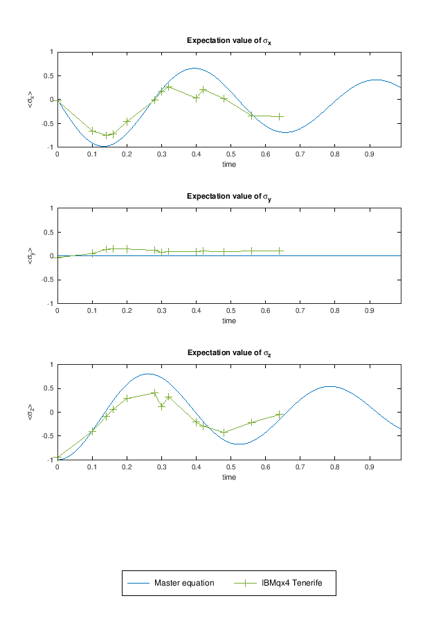
Here $M^{+}$ and $M^{0}$ are given by Eqn (LABEL:eq_coefficients). Figure 1 compares the theoretical results given by the master equation Eqn (9) and the results obtained with the IBMqx4 Tenerife quantum computer.

Figure 1: Calculated expectation values for the Pauli spin operators for the two-level atom, using parameters $\kappa=1$, $\omega=0$ and $\Omega=12$. Results are plotted for the master equation Eqn (9), and calculations on the actual IBMqx4 Tenerife quantum computer. The results of the master equation are obtained using a time step $\lambda^{2}=0.01$. The IBMqx4 curve consists of collected results of experiments with time steps $\lambda^{2}=0.16$, $0.14$, and $0.10$, each averaged over 10240 runs.

4.2 Homodyne quantum filter

We now turn to the situation where we are not simply tracing over the field, but condition on observations made in the field. Suppose that for $l=1,2,3,4$, we have observed $\lambda*\sigma_{x}$ in the field:

$$\Delta Y(l):=\lambda*\mbox{"the outcome of the\ }\sigma_{x}\mbox{-measurement of the\ }l\mbox{th field qubit"}.$$

Physically, this corresponds to the case where we observe the field with a homodyne detection setup after the interaction with the two-level atom. We can condition the time evolution of the density matrix on an observed homodyne photo current detection record. The conditioned density matrix obeys the following discrete quantum filtering equation for homodyne detection [6, Section 5.2, page 274]

$$\begin{split}\Delta\rho_{l}=\mathcal{L}(\rho_{l-1})\lambda^{2}+\frac{\mathcal{J}(\rho_{l-1})-\mbox{tr}[\mathcal{J}(\rho_{l-1})]\Big{(}\rho_{l-1}+\lambda^{2}\mathcal{L}(\rho_{l-1})\Big{)}}{1-\lambda^{2}\mbox{tr}[\mathcal{J}(\rho_{l-1})]^{2}}\Big{(}\Delta Y(l)-\mbox{tr}[\mathcal{J}(\rho_{l-1})]\lambda^{2}\Big{)},\end{split}$$ (11)

where $\mathcal{L}$ is given by Eqn (10) and $\mathcal{J}$ and the initial state $\rho_{0}$ are given by

$$\mathcal{J}(\rho):=M^{+}\rho+\rho{M^{+}}^{*}+\lambda^{2}M^{+}\rho{M^{0}}^{*}+\lambda^{2}M^{0}\rho{M^{+}}^{*},\ \ \ \ \rho_{0}=\begin{pmatrix}0&0\\ 0&1\end{pmatrix},$$

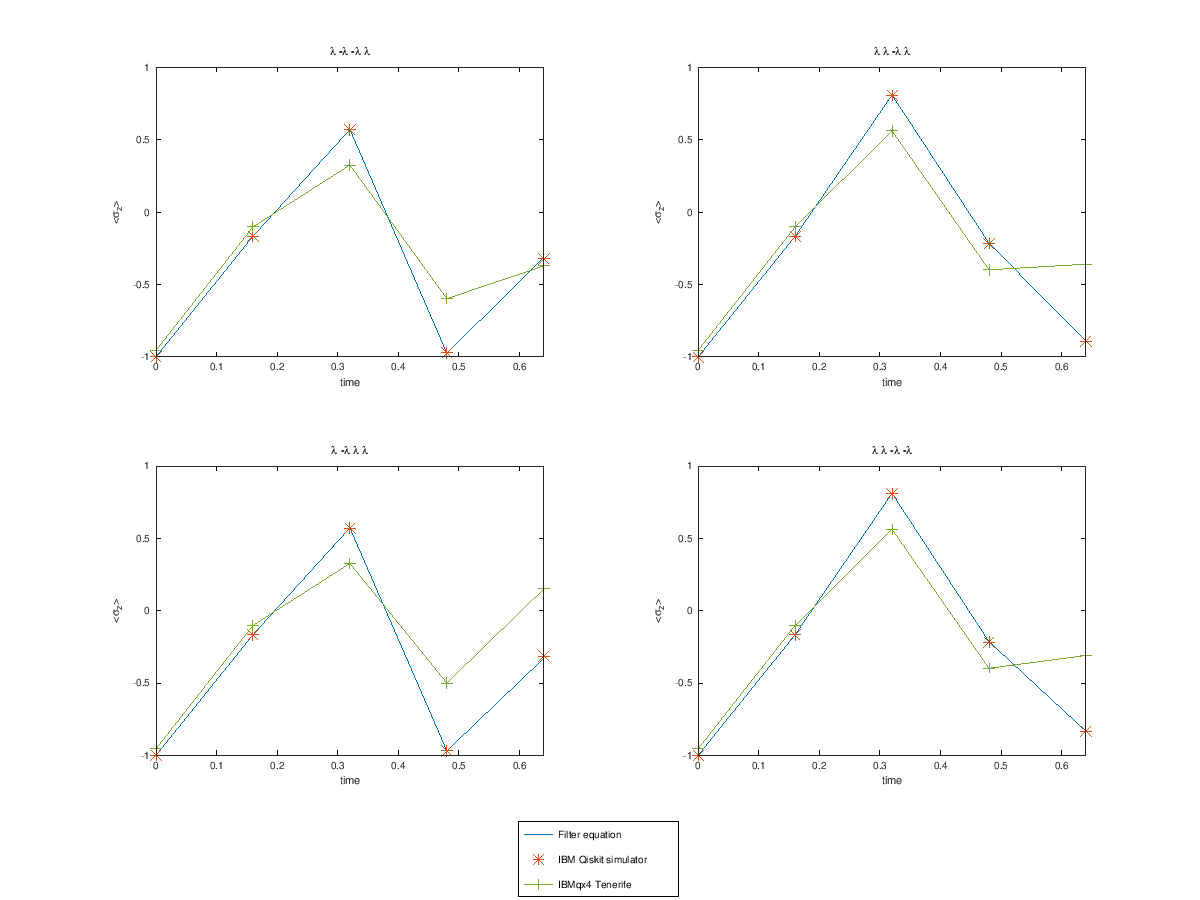
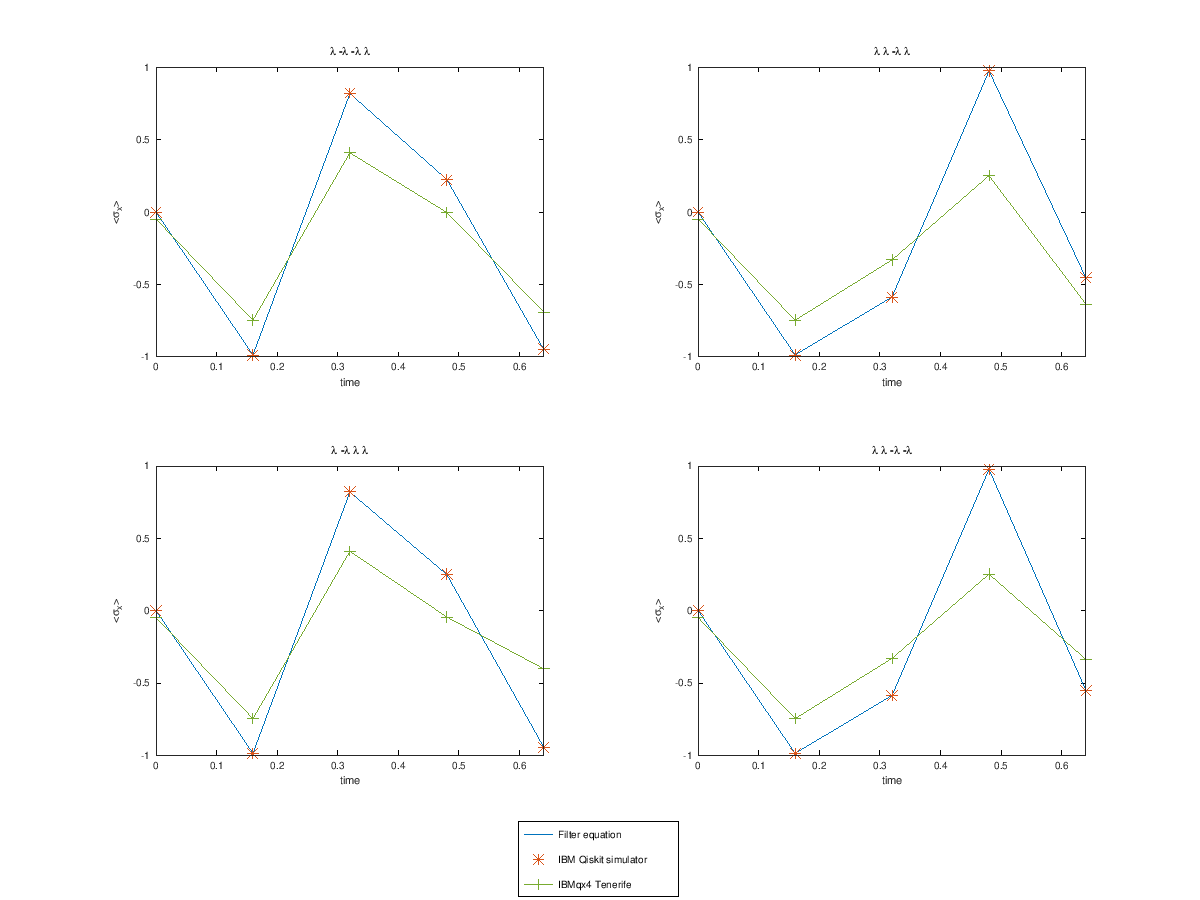
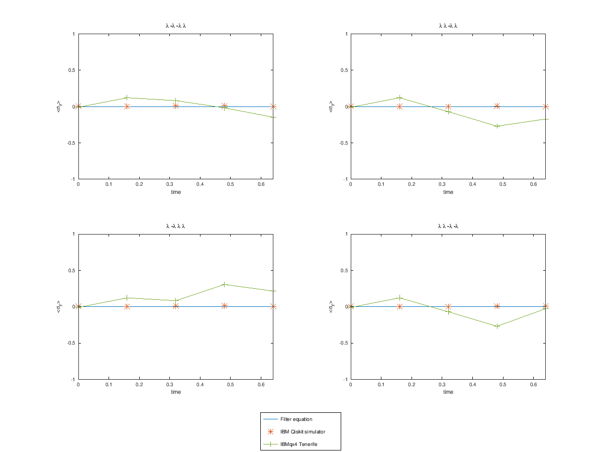
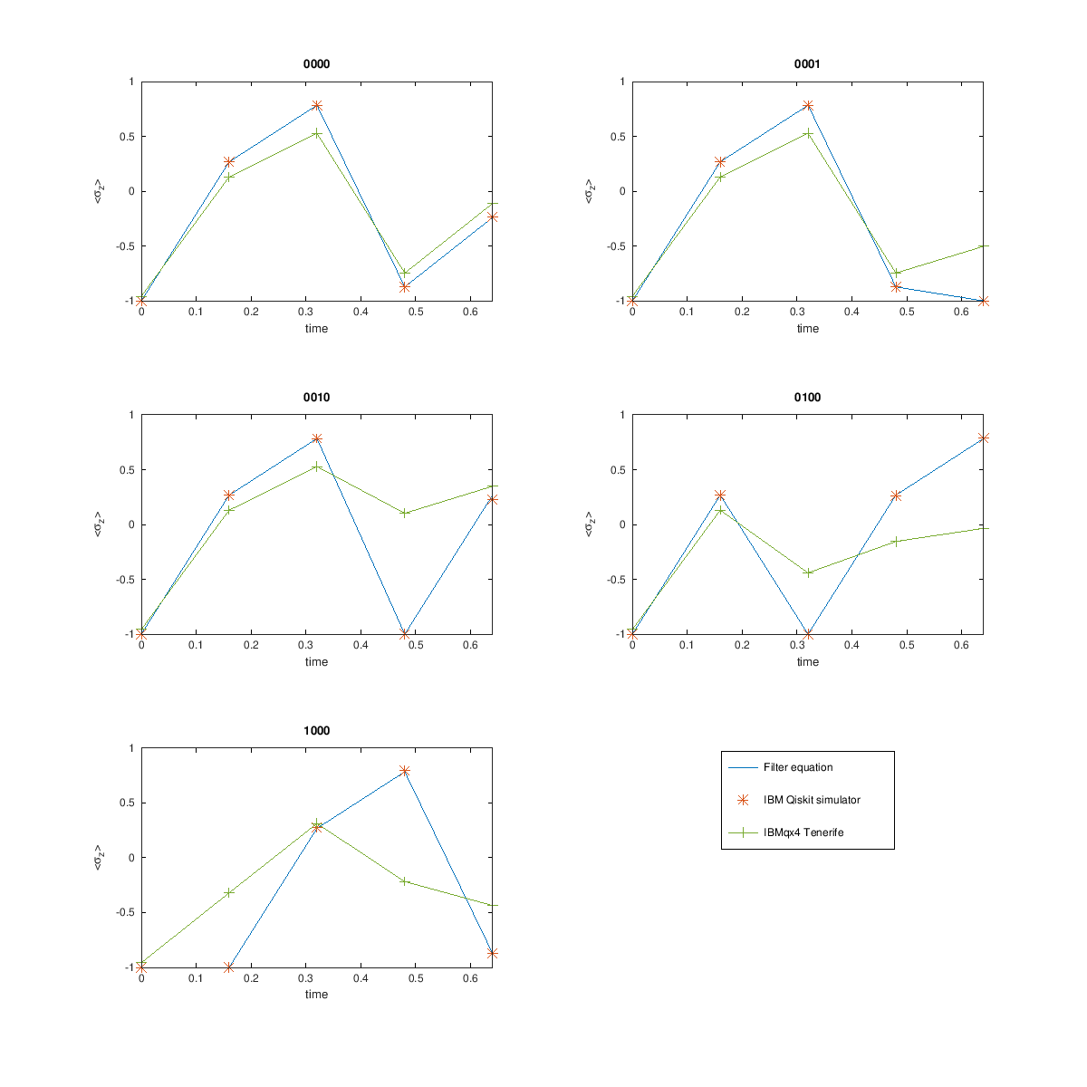
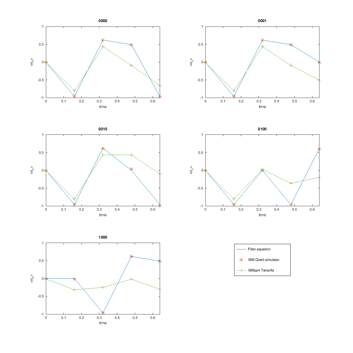
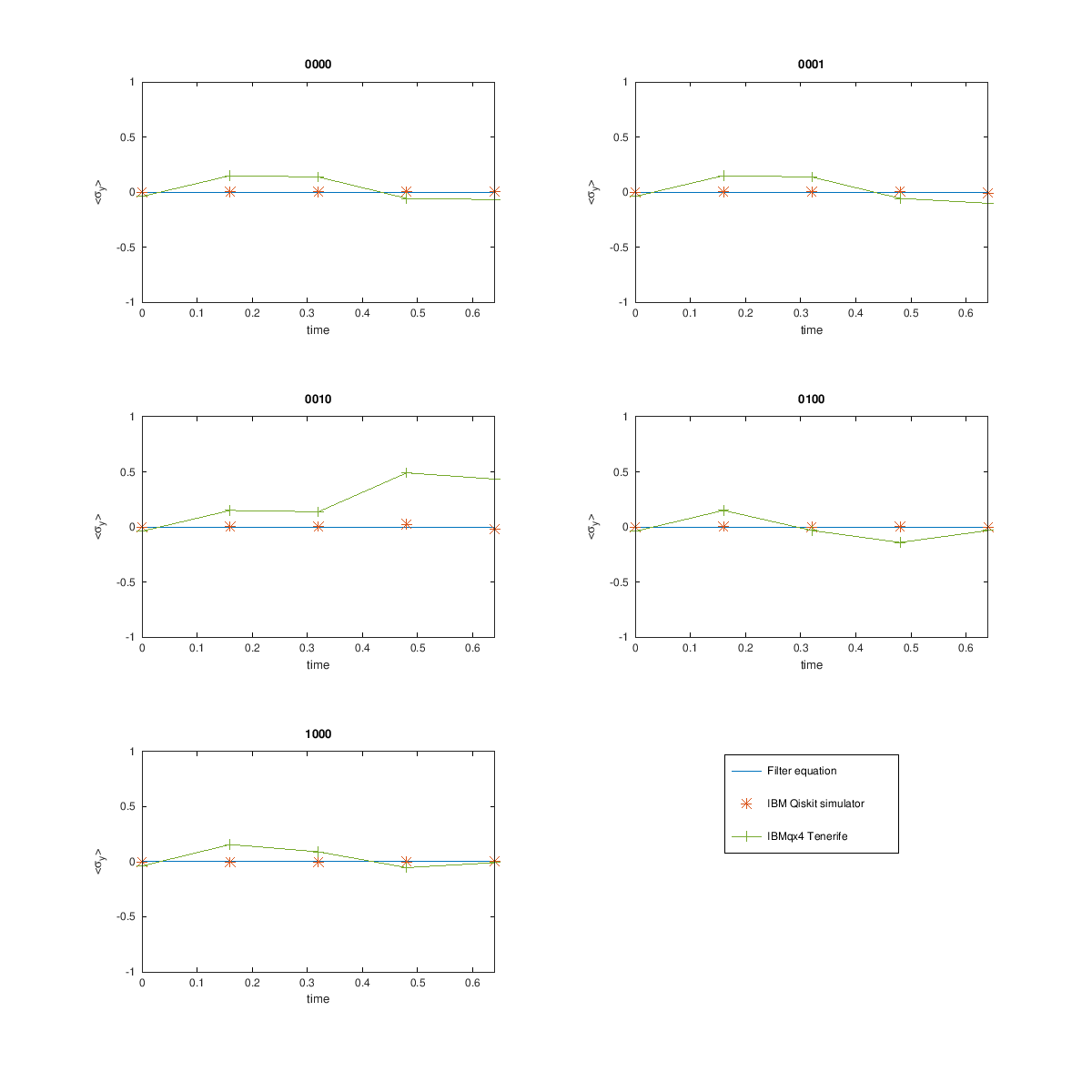
Here $M^{+}$ and $M^{0}$ are given by Eqn (LABEL:eq_coefficients). Figures 2, 3 and 4 compare the theoretical results given by the quantum filter equation Eqn (11) and the results obtained with the IBM Qiskit [1] simulator and the IBMqx4 Tenerife quantum computer.

Figure 2: Time evolution of the expectation value of the Pauli $\sigma_{z}$ operator of the two-level atom, in the homodyne detection scheme, for the four trajectories that have accumulated the most statistics. The trajectory is given by the title above the plots, which shows $\Delta Y$. The filter equation results are from Eqn (11). The IBMqx4 results are averaged over 10,240 runs. The simulator results are obtained from the IBM Qiskit simulator, using the same quantum assembly code that was used on the IBMqx4 Tenerife computer, and are averaged over 102,400 runs.

Figure 3: As Figure 2, for the $\sigma_{x}$ operator.

Figure 4: As Figure 2, for the $\sigma_{y}$ operator.

4.3 Counting quantum filter

Finally, we turn to the situation where we condition on having observed $\sigma_{+}\sigma_{-}$ in the field for $l=1,2,3,4$. That is, we have the following observations:

$$\Delta Y(l)=\frac{1+\mbox{"the outcome of the\ }\sigma_{z}\mbox{-measurement of the\ }l\mbox{th field qubit"}}{2}.$$

Physically, this corresponds to the case where we observe the field with a photo detector after the interaction with the two-level atom. We can condition the time evolution of the density matrix on an observed photo detection record. The conditioned density matrix obeys the following discrete quantum filtering equation for photon counting [6, Section 5.3, page 276]

$$\begin{split}\Delta\rho_{l}{}&=\mathcal{L}(\rho_{l-1})\lambda^{2}+\frac{\frac{M^{+}\rho_{l-1}{M^{+}}^{*}}{\mbox{tr}[\rho_{l-1}{M^{+}}^{*}M^{+}]}-\rho_{l-1}-\lambda^{2}\mathcal{L}(\rho_{l-1})}{1-\lambda^{2}\mbox{tr}[\rho_{l-1}{M^{+}}^{*}M^{+}]}\Big{(}\Delta Y(l)-\mbox{tr}[\rho_{l-1}{M^{+}}^{*}M^{+}]\lambda^{2}\Big{)},\\ \rho_{0}{}&=\begin{pmatrix}0&0\\ 0&1\end{pmatrix}.\end{split}$$ (12)

Here $M^{+}$ is given by Eqn (LABEL:eq_coefficients). Figures 5, 6 and 7 compare the theoretical results given by the quantum filter equation Eqn (12) and the results obtained with the IBM Qiskit simulator and the IBMqx4 Tenerife quantum computer.

Figure 5: Time evolution of the expectation value of the Pauli $\sigma_{z}$ operator of the two-level atom, in the photon counting scheme, for the case where no photons were detected (0000), and where a single photon was detected after the fourth (0001), third (0010), second (0100) and first (1000) time step. The filter equation results are from Eqn (12). The IBMqx4 results are averaged over 10,240 runs. The simulator results are obtained from the IBM Qiskit simulator, using the same quantum assembly code that was used on the IBMqx4 Tenerife computer, and are averaged over 102,400 runs.

Figure 6: As Figure 5, for the $\sigma_{x}$ operator.

Figure 7: As Figure 5, for the $\sigma_{y}$ operator.

5 Conclusion

In these notes we have shown that it is fairly straightforward to implement quantum stochastic differential equations on a quantum computer. The mathematical theory [16, 19, 17, 2, 5, 6] behind the necessary discretization of the equations is well worked out and easily translated into a quantum circuit. It is possible with the very limited capacity of the currently available quantum computers to simulate some simple quantum optical features described by a QSDE (e.g. a Rabi oscillation).

We have also seen that the filter equations are to a large extent correctly reproduced on the IBMqx4 Tenerife quantum computer. This provides confidence that the (quantum) correlations between the atom and the field are accounted for correctly. This opens the door to fully coherent simulations of systems that interact with the field at different points, even including fully coherent feedback loops [11, 10]. Naturally, this is only possible when quantum computers are available with more and more reliable qubits.

As can be seen in Figures 5 and 6, the time evolution between counts in the photon counting scheme seems to be accounted for correctly, however, the jump operation does not seem to be accurate to the theory. This can be understood though: there are relatively few jumps and there is already quite a bit of noise on the results when the field is in the vacuum state. This means there is an identity component in the jump operator that leads to a deviation from the theory (in which this noise is not present, but could be modeled).

With respect to the discrete quantum filtering equations [6], we note that they completely coincide with the IBM Qiskit simulator results. However, they are much less computationally intensive and could still be used if the number of qubits is larger than the simulator can deal with. Note, however, that in the simulator it is also possible to recycle the field qubits after they have been measured. This is currently not yet possible on the real IBMQ hardware.

It will be interesting to see future quantum computers simulate more complex benchmark problems originating from quantum optics.

References

- [1] G. Aleksandrowicz, T. Alexander, P. Barkoutsos, L. Bello, Y. Ben-Haim, D. Bucher, F. J. Cabrera-Hernádez, J. Carballo-Franquis, A. Chen, C.-F. Chen, J. M. Chow, A. D. Córcoles-Gonzales, A. J. Cross, A. Cross, J. Cruz-Benito, C. Culver, S. D. L. P. González, E. D. L. Torre, D. Ding, E. Dumitrescu, I. Duran, P. Eendebak, M. Everitt, I. F. Sertage, A. Frisch, A. Fuhrer, J. Gambetta, B. G. Gago, J. Gomez-Mosquera, D. Greenberg, I. Hamamura, V. Havlicek, J. Hellmers, Ł. Herok, H. Horii, S. Hu, T. Imamichi, T. Itoko, A. Javadi-Abhari, N. Kanazawa, A. Karazeev, K. Krsulich, P. Liu, Y. Luh, Y. Maeng, M. Marques, F. J. Martín-Fernández, D. T. McClure, D. McKay, S. Meesala, A. Mezzacapo, N. Moll, D. M. Rodríguez, G. Nannicini, P. Nation, P. Ollitrault, L. J. O’Riordan, H. Paik, J. Pérez, A. Phan, M. Pistoia, V. Prutyanov, M. Reuter, J. Rice, A. R. Davila, R. H. P. Rudy, M. Ryu, N. Sathaye, C. Schnabel, E. Schoute, K. Setia, Y. Shi, A. Silva, Y. Siraichi, S. Sivarajah, J. A. Smolin, M. Soeken, H. Takahashi, I. Tavernelli, C. Taylor, P. Taylour, K. Trabing, M. Treinish, W. Turner, D. Vogt-Lee, C. Vuillot, J. A. Wildstrom, J. Wilson, E. Winston, C. Wood, S. Wood, S. Wörner, I. Y. Akhalwaya, and C. Zoufal. Qiskit: An open-source framework for quantum computing, 2019.
- [2] S. Attal and Y. Pautrat. From repeated to continuous quantum interactions. Annales Henri Poincaré, 7:59–104, 2006.
- [3] V. P. Belavkin. Quantum stochastic calculus and quantum nonlinear filtering. J. Multivar. Anal., 42:171–201, 1992.
- [4] L. Bouten, R. van Handel, and M. James. An introduction to quantum filtering. SIAM J. Control Optim., 46:2199–2241, 2007.
- [5] L. M. Bouten and R. van Handel. Discrete approximation of quantum stochastic models. J. Math. Phys., 49:102109, 2008.
- [6] L. M. Bouten, R. van Handel, and M. James. A discrete invitation to quantum filtering and feedback control. SIAM Review, 51:239–316, 2009.
- [7] T. A. Brun. A simple model of quantum trajectories. Am. J. Phys., 70:719–737, 2002.
- [8] H. J. Carmichael. An Open Systems Approach to Quantum Optics. Springer-Verlag, Berlin Heidelberg New-York, 1993.
- [9] E. B. Davies. Quantum stochastic processes. Commun. Math. Phys., 15:277–304, 1969.
- [10] J. Gough and M. James. Quantum feedback networks: Hamiltonian formulation. Commun. Math. Phys., 287:1109–1132, 2009.
- [11] J. Gough and M. James. The series product and its application to quantum feedforward and feedback networks. IEEE Trans. Aut. Control, 54:2530–2544, 2009.
- [12] J. Gough and A. Sobolev. Stochastic Schrödinger equations as limit of discrete filtering. Open Syst. Inf. Dyn., 11:235–255, 2004.
- [13] J. A. Gross, C. M. Caves, G. J. Milburn, and J. Combes. Qubit models of weak continuous measurements: markovian conditional and open-system dynamics. Quantum Science and Technology, 3(2):024005, 2018.
- [14] R. L. Hudson and K. R. Parthasarathy. Quantum Itô’s formula and stochastic evolutions. Commun. Math. Phys., 93:301–323, 1984.
- [15] IBM. The IBM Q experience. https://quantumexperience.ng.bluemix.net/qx. Accessed 23 November 2018.
- [16] B. Kümmerer. Markov dilations on -algebras. J. Funct. Anal., 63:139–177, 1985.
- [17] J. M. Lindsay and K. R. Parthasarathy. The passage from random walk to diffusion in quantum probability ii. Sankhya: The Indian journal of statistics, 50:151–170, 1988.
- [18] M. Nielsen and I. Chuang. Quantum Computation and Quantum Information. Cambridge University Press, 2000.
- [19] K. R. Parthasarathy. The passage from random walk to diffusion in quantum probability. Journal of applied probability, special volume 25A:151–166, 1988.