FLaREON: a fast computation of $\mathrm{Ly}\alpha$ escape fractions and line profiles

Abstract

We present FLaREON (Fast Lyman-Alpha Radiative Escape from Outflowing Neutral gas), a public Python package that delivers fast and accurate $\mathrm{Ly}\alpha$ escape fractions and line profiles over a wide range of outflow geometries and properties. The code incorporates different algorithms, such as interpolation and machine learning to predict $\mathrm{Ly}\alpha$ line properties from a pre-computed grid of outflow configurations based on the outputs of a Monte Carlo radiative transfer code. Here we describe the algorithm, discuss its performance and illustrate some of its many applications. Most notably, FLaREON can be used to infer the physical properties of the outflowing medium from an observed $\mathrm{Ly}\alpha$ line profile, including the escape fraction, or it can be run over millions of objects in a galaxy formation model to simulate the escape of $\mathrm{Ly}\alpha$ photons in a cosmological volume.

1 Introduction

Since the first evidence of star forming galaxies emitting $\mathrm{Ly}\alpha$ photons (Steidel et al., 1996; Hu et al., 1998), more than two decades ago, observational campaigns targeting these sources have developed to become a standard technique to identify high redshift galaxies (e.g. Rhoads et al., 2000; Malhotra & Rhoads, 2002; Konno et al., 2016; Sobral et al., 2017; Ouchi et al., 2018). However, we are still far from a comprehensive understanding of this galaxy population due to the complex radiative transfer (RT) processes that $\mathrm{Ly}\alpha$ photons experience (see Dijkstra, 2017, for a review).

The $\mathrm{Ly}\alpha$ RT in astrophysical media can be addressed analytically for static, simplified geometries (e.g. Harrington, 1973; Neufeld, 1990). However, the limited validity of such approach encouraged the development of numerical Monte Carlo radiative transfer (MCRT) codes. In this approach, $\mathrm{Ly}\alpha$ photons are tracked individually as they interact in arbitrarily complex 3D gas geometries. As a result, information about the fraction of photons that manage to escape, $f_{\rm esc}^{\rm Ly\alpha}$, and their resulting line profile is computed (Ahn et al., 2000; Zheng & Miralda-Escudé, 2002; Ahn, 2003; Verhamme et al., 2006; Orsi et al., 2012; Verhamme et al., 2012; Laursen et al., 2009; Gronke et al., 2016).

One drawback of the MCRT technique is given by the time it takes to simulate an appropriate number of photons to obtain statistically significant results. The mean number of scattering events scales roughly proportionally with the $\mathrm{Ly}\alpha$ rest-frame optical depth of the medium (Harrington, 1973). Hence, the computational time can vary by several orders of magnitude depending on the physical configuration probed. Typically, approximately $10^{4}-10^{5}$ photons are needed to retrieve the shape of the $\mathrm{Ly}\alpha$ line profile with reasonable resolution. Such exercise becomes quickly prohibitively expensive when running MCRT codes for multiple configurations. One scenario where this requirement is needed is in $\mathrm{Ly}\alpha$ line profile fitting (e.g. Mejias et al., in prep). Another example is to incorporate the $\mathrm{Ly}\alpha$ properties of objects in a galaxy formation model run over a cosmological box (e.g. Orsi et al., 2012; Garel et al., 2012; Gurung-López et al., 2019b)

Here we address the problem described above by presenting FLaREON, a publicly available Python package able to quickly predict multiple Lyman-$\alpha$ line profiles and escape fractions with high accuracy. The basis of the results is a grid of configurations computed previously using the MCRT code LyaRT (Orsi et al., 2012).The outline of this work is as follows. In §2 we present FLaREON. In §3 we test its accuracy and in §4 we briefly explain how to exploit FLaREON. In §5 we illustrate some possible applications. Finally, we present our conclusions in §6.

Figure 1: The $\mathrm{Ly}\alpha$ line properties in different geometries. The left panels show a cartoon of the Biconical wind, Thin shell and Galactic wind. The middle panels show the $\mathrm{Ly}\alpha$ escape fraction as a function of dust optical depth of absorption $\tau_{a}$ for the three geometries and outflow configuration as shown in the legend. The right panels show examples of $\mathrm{Ly}\alpha$ line profiles for the configurations described in the legend.

2 Code description

FLaREON  makes use of a grid of configurations run with the Monte Carlo radiative transfer code LyaRT (Orsi et al., 2012). This grid covers three different outflow geometries and a wide range of gas properties. The goal of the code is to deliver a user-friendly public Python package able to predict thousands of Lyman-$\alpha$ line profiles and $f_{\rm esc}^{\rm Ly\alpha}$ in seconds with minimal user input.

2.1 Outflow Geometries

There are three different outflow geometries implemented in FLaREON: Thin shell, Wind, and Biconical wind. They all feature an empty inner cavity and an isotropic monochromatic source of $\mathrm{Ly}\alpha$ photons is placed in the centre. Other works in the literature include a non-monocromatic intrinsic $\mathrm{Ly}\alpha$ line profile that produce some modifications in the emerging line profile (e.g. Verhamme et al., 2006). We plan to implement arbitrary intrinsic line profiles in a future update. In all geometries, dust follows the gas density. The dust optical depth is defined as

$$\centering\tau_{a}=(1-A_{{\rm Ly}\alpha})\frac{E_{\odot}}{Z_{\odot}}{N_{H}}Z,\@add@centering$$ (1)

where $E_{\odot}=1.77\times 10^{-21}{\rm cm^{-2}}$ (Silva et al., 1998; Orsi et al., 2012) is the ratio $\tau_{a}/N_{H}$ for solar metallicity, $A_{Ly\alpha}=0.39$ is the albedo at the Ly$\alpha$ wavelength, $Z_{\odot}=0.02$ (Granato et al., 2000), $Z$ is the gas metallicity and $N_{\rm H}$ is the neutral hydrogen column density. We assume the temperature of the gas is constant at $T=10000~{}{\rm K}$.

The Thin shell and Wind geometries are described in detail in Orsi et al. (2012) and Gurung-López et al. (2019b). In the following we briefly describe them. The Biconical wind described below is slightly different to that presented in Gurung-López et al. (2019b).

1. Thin shell: an isothermal uniform neutral hydrogen distributed in a thin layer with a radial expansion velocity ${\rm V_{exp}}$. This geometry has been widely used in the literature to study the escape of $\mathrm{Ly}\alpha$ photons (e.g. Zheng & Miralda-Escudé, 2002; Ahn, 2004; Verhamme et al., 2006; Orsi et al., 2012).

2. Wind: a spherical isothermal distribution of neutral hydrogen with radial expansion velocity $V_{\rm exp}$ as implemented in Orsi et al. (2012). This geometry exhibits an empty spherical cavity with radius $R_{\rm Wind}$ (analogously to $R_{\rm inner}$ in the Thin shell) and a radially decreasing number density profile.

3. Biconical wind: this is a combination of an outflow with expanding wind geometry and a static isothermal uniform medium. The expanding wind outflow with $V_{\rm exp,in}>0$ and $N_{\rm H,in}$ is confined in $\theta<\theta_{\rm cone}$ and $\theta>\pi-\theta_{\rm cone}$, where $\theta_{\rm cone}$ is measured from the polar axis. We define $\theta_{\rm cone}=\pi/4$. For $\theta_{\rm cone}<\theta<\pi-\theta_{\rm cone}$, the medium is static ($V_{\rm exp,out}=0$) with column density ${N_{\rm H,out}}=f\times{N_{\rm H,in}}$. Here we arbitrarily set $f=10^{3}$. This value of $f$ assures that the slab is optically thick in comparison to the bicone, thus most of the photones escape through the bicone. The column density of this geometry $N_{\rm H}$ is

   $$\centering N_{\rm H}=(1-\cos\theta_{\rm cone}){N_{\rm H,in}}+\cos\theta_{\rm cone}{N_{\rm H,out}}\@add@centering$$ (2)

   where ${N_{\rm H,in}}$ corresponds to the column density of the Wind geometry (see Gurung-López et al., 2019b).

Figure 2: Distribution of the relative difference between the output of LyaRT and the predictions of FLaREON for 300 random outflow configurations using the Thin shell geometry. The result with the analytical expressions is shown in blue. The result with the machine learning algorithm (labeled as ’ML’) using the raw outputs of LyaRT (labeled as ’V’) and using the best fitting parameters of equation 9 (labeled as ’P’) are plotted in red and yellow respectively. Additionally, the algorithms using linear interpolation (labeled as ’Inter’) and the raw output of LyaRT (’V’) and using the fitting parameters (’P’) are shown in purple and green respectively. The legend displays the standard deviation of each FLaREON algorithm.

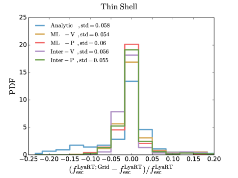
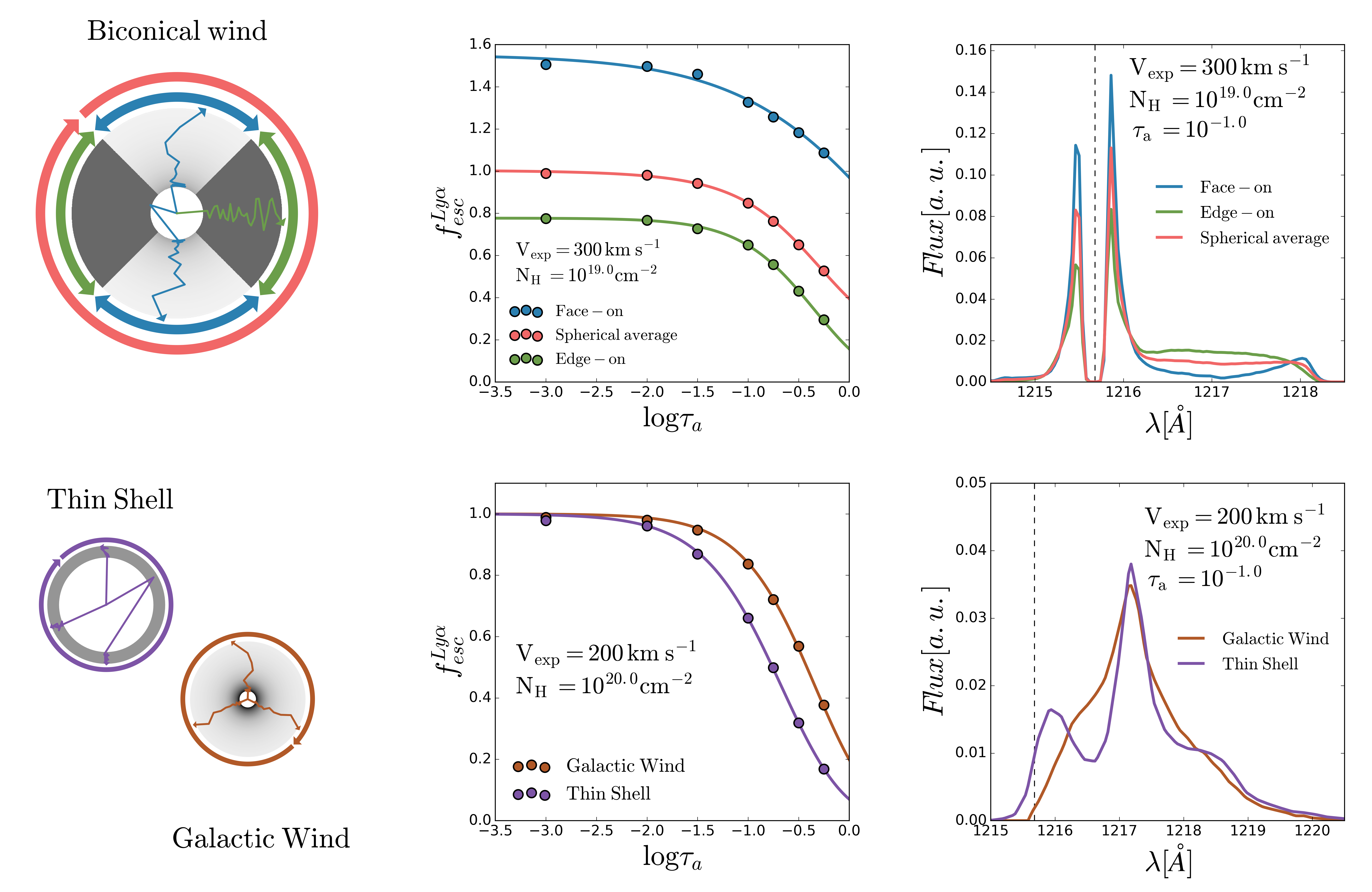
Fig. 1 illustrates the main features of the three geometries described. For the Biconical wind, photons scattering through the dense and static torus are less likely to escape compared to those traveling through the thin outflow. The dipolar nature of the scattering of $\mathrm{Ly}\alpha$ photons through a neutral hydrogen medium makes them likely to back-scatter within the inner cavity until they escape through the thin medium. For $\theta_{\rm cone}=\pi/4$, $\sim 70\%$ of the photons are emitted towards the thick torus and only a few ($\sim 30\%$) towards the bicone.

When treating the biconical geometry, it is important to note that $f_{\rm esc}^{\rm Ly\alpha}$ can be define for an arbitrary angular aperture $\Delta\gamma$ as

$$\centering f_{\rm esc}^{\rm Ly\alpha}(\Delta\gamma)={{N_{\rm escaped}(\Delta\gamma)}\over{N_{\rm emitted}(\Delta\gamma)}}\@add@centering$$ (3)

where $N_{\rm emitted}(\Delta\gamma)$ is the number of photons initially sent towards the angle aperture $\Delta\gamma$ and ${N_{\rm escaped}(\Delta\gamma)}$ is the number of photons that manage to escape through that set of directions. Note that for the non-biconical Galactic wind and the Thin shell this expression is valid and $\Delta\gamma$ is every line of sight ($4\pi$).

The bicone geometry is not spherically symmetric, thus its $f_{\rm esc}$ depends on the line of sight. In the case of the face-on bicone, the escape fraction presented in our work corresponds to the $f_{\rm esc}^{\rm Ly\alpha}(\Delta\gamma_{b})$ where $\Delta\gamma_{b}$ is the angular aperture $\theta<\pi/4\cup\theta>3\pi/4$ and $\phi\in[0,2\pi)$. In other words, we define the face-on biconical escape fraction as the number of photons that escape through the bicone divided by the number of photons emitted towards the bicone. In a similar way, we define the edge-on escape fraction as $f_{\rm esc}^{\rm Ly\alpha}(\Delta\gamma_{s})$ where $\Delta\gamma_{s}$ is the angular aperture $\theta\in[\pi/4,3\pi/4]$ and $\phi\in[0,2\pi)$.

The inclination of the Biconical wind with respect to the observer leads to different escape fractions. This is shown in the middle panel of Fig. 1 by computing the escape fraction $f_{\rm esc}^{\rm Ly\alpha}$ of $\mathrm{Ly}\alpha$ photons though the bicone (face-on) or through the torus (edge-on). The escape fraction is defined as the ratio between the number of photons that escape through a given direction over the number of photons emitted towards that direction. The three cases shown in Fig. 1 (edge-on, face-on and the spherically average) show significant differences. If the geometry is observed face-on, $f_{\rm esc}^{\rm Ly\alpha}$ reaches values greater than 1, while if it is edge-on $\mbox{$f_{\rm esc}^{\rm Ly\alpha}$}<1$ even if there is no dust. This is caused by the large optical depth of the torus that beams the $\mathrm{Ly}\alpha$ photons towards the bicone. In the spherically averaged $f_{\rm esc}^{\rm Ly\alpha}$  reaches unity for dust-free configurations.

The right panel of Fig. 1 shows the resulting line profiles for the bicone at the three different orientations. The differences in the line profile between the three cases reflect the different scattering histories of photons escaping through the outflow or the thick torus.

Fig. 1 also shows the corresponding $f_{\rm esc}^{\rm Ly\alpha}$ and line profiles for the Thin shell and Wind, respectively. Here, there is no difference in the escape of $\mathrm{Ly}\alpha$ photons due to the orientation of the outflows.

Figure 3: Left : Normalized distribution of the KS statistic of the $\mathrm{Ly}\alpha$ line profile computed by LyaRT and predicted by FLaREON in the same 300 random {$\rm V_{exp}$, $\rm N_{H}$, $\tau_{a}$} combinations for the Thin shell (yellow), the Wind (red), and the bicone face-on (blue) and edge-on (green). Right : comparison between the LyaRT output (solid black lines) and FLaREON predictions (colored solid lines) in some of the 300 random configurations. We show Thin shell, Wind and Bicone configurations from left to right. Additionally, in the legend indicates the KS between the LyaRT and FLaREON line profiles.

2.2 Monte Carlo configuration grids

FLaREON is based in the outputs of LyaRT in a grid of configurations spanning a wide range of phyisical properties. We build two grids for each outflow geometry; one to infer $f_{\rm esc}^{\rm Ly\alpha}$ and another to predict $\mathrm{Ly}\alpha$ line profiles. For the $f_{\rm esc}^{\rm Ly\alpha}$, the grids are constructed using a number of photons $N_{p}=10^{4}$. Hence, the lowest value of $f_{\rm esc}^{\rm Ly\alpha}$ computed is $10^{-4}$. For the line profile grids, we use instead $N_{p}=10^{5}$, since we need more photons to fully recover the shape of the resulting line profiles. In order to speed-up the computational time in the latter case, we implement an acceleration procedure to dismiss scattering events that result in frequency changes below a critical value of $x_{\rm crit}=3$, where $x$ is the frequency of photons in Doppler units (see, e.g. Dijkstra et al., 2006; Laursen & Sommer-Larsen, 2007; Orsi et al., 2012). Those scattering events have no significant impact on the resulting line profile, but skipping them can improve the performance of the Monte Carlo calculation by orders of magnitude. Since the bicone geometry is split into two lines of sight we increased the number of photons to $10^{5}$ and $10^{6}$ for the $f_{\rm esc}^{\rm Ly\alpha}$ and line profile grids, respectively.

The $V_{\rm exp}$-$\log N_{\rm H}$ parameter space covered in the grids is defined as follows:

$$\centering{V_{\rm exp}[km\;s^{-1}]}=\left\{\begin{array}[]{c l l }\left[10\;,100\right]\;,&{\Delta{V_{\rm exp}}=10\;{\rm km\;s^{-1}}}\\ \left[100\;,1000\right]\;,&{\Delta{V_{\rm exp}}=50\;{\rm km\;s^{-1}}}\end{array}\right.\@add@centering$$ (6)

where $\Delta{V_{\rm exp}}$ is the step between evaluations. Additionally, the neutral hydrogen column density $N_{\rm H}$ is mapped in bins of $\Delta\log{N_{\rm H}}=0.25$ and spans the following range:

$$\centering{\log N_{\rm H}{\rm[cm^{-2}]}}=\left[17\;,22\right]\;\;,\;\;{\Delta{\log N_{\rm H}[{\rm cm^{-2}]}}=0.25}\@add@centering$$ (7)

The values of dust optical depth $\tau_{\rm a}$ where the grid is sampled are different for the $f_{\rm esc}^{\rm Ly\alpha}$ and line profile grids. We have checked that a sparse sampling of $f_{\rm esc}^{\rm Ly\alpha}$ is sufficient to deliver good results. These values are $\log\tau_{\rm a}=\left[-3.0\;,-2.0\;,-1.5\;,-1.0\;,-0.75\;,-0.5\;,-0.25\;,\;0.0\right]$. The line profile grids, on the other hand, spans a wider range and more frequently in $\tau_{\rm a}$ to track properly the evolution with dust optical depth of the $\mathrm{Ly}\alpha$ line profile. We cover the low dust range with higher density as we found that the evolution is stronger in this range. Finally, the dust optical depth values are

$$\centering{\log\tau_{\rm a}}=\left\{\begin{array}[]{c l l }\left[-3.75\;,-1.500\right]\;,&{\Delta\log\tau_{\rm a}=0.25}\\ \left[-1.50\;,-0.125\right]\;,&{\Delta\log\tau_{\rm a}=0.125}\\ \end{array}\right.\@add@centering$$ (8)

where $\Delta\log\tau_{\rm a}$ is the step between evaluations.

All together, the total number of configurations sampled for each geometry is 4704 and 12348 for the $f_{\rm esc}^{\rm Ly\alpha}$ and line profile grids, respectively.

2.3 Predicting the Lyman-$\alpha$ properties.

FLaREON allows the user to choose among three different methods to compute the $f_{\rm esc}^{\rm Ly\alpha}$from the outflow properties:

Figure 4: Correlation between some line profile properties produced by the Bicone, Galactic wind and Thin shell geometries from left to right. Top : half of the separations between the red and the blue peaks in the line profile as a function of shift of the red peak from $\mathrm{Ly}\alpha$ wavelength. Only configurations producing double peak profiles were taken into account for this panel. Bottom : full width half maximum of the red peak as a function of the shift of the red peak from $\mathrm{Ly}\alpha$ wavelength . Only configurations producing line profiles without a blue peak were taken into account for this panel. In every panel, the $\rm N_{H}$ is color coded. The one-to-one relation is plotted in black dashed lines to guide the eye.

1. The first method uses directly the values of $f_{\rm esc}^{\rm Ly\alpha}$ given by LyaRT to build a multi-dimensional linear interpolation grid or to train a machine learning algorithm. For the latter, FLaREON incorporates ’extra trees’, ’random forest’ and ’k-nearest neighbors’, using the Python module scikit-learn (Pedregosa et al., 2011).
   

2. The second method consists in using a parametric equation that links $f_{\rm esc}^{\rm Ly\alpha}$ and one or several gas properties. In particular, we fit the $f_{\rm esc}^{\rm Ly\alpha}$computed by LyaRT as a function of the dust optical depth in each node of the $V_{\rm exp}$-$\log N_{\rm H}$ space to the function inspired by Neufeld (1990) :

   $$\centering f_{\rm esc}^{\rm Ly\alpha}=k_{3}\left[\cosh\sqrt{k_{1}\tau_{\rm a}^{k_{2}}}\right]^{-1},\@add@centering$$ (9)

   where $k_{1}$, $k_{2}$ and $k_{3}$ are free parameters. Note that $k_{3}=1$ in the Thin shell and Wind geometries since if there is no dust $f_{\rm esc}^{\rm Ly\alpha}=1$. However, in the Bicone geometry, as we divide in edge-on and face-on, in general, $k_{3}\neq 1$ as discussed in §2.1. The best fitting parameters are then used to build the linear interpolated grid or to train the machine learning algorithms in this mode.
   

3. The third method consists on an updated version of the analytic $f_{\rm esc}^{\rm Ly\alpha}$ expressions described in Gurung-López et al. (2019b). Those $f_{\rm esc}^{\rm Ly\alpha}$ parametric equations have been recalibrated for the Thin shell and Wind in our grid, which is denser and wider in $V_{\rm exp}$ and $N_{\rm H}$. Due to the complexity of $f_{\rm esc}^{\rm Ly\alpha}$ in the face-on and edge-on configurations, FLaREON does not include any analytic expression for the biconical outflow.
   

To address the problem of predicting $\mathrm{Ly}\alpha$ line profiles, analytic expressions and machine learning algorithms perform poorly compared to a multi-dimensional linear interpolation of the LyaRT outputs. Hence, unlike the case of the $f_{\rm esc}^{\rm Ly\alpha}$, the $\mathrm{Ly}\alpha$ line profiles are computed using only a multi-linear interpolation of the grids.

3 Validation of the code

Here we compare the performance of different methods to obtain $f_{\rm esc}^{\rm Ly\alpha}$. We compute 300 random values for $V_{\rm exp}$, $\log N_{\rm H}$ and $\log\tau_{\rm a}$ using a Latin hypercube algorithm to populate randomly and homogeneously the three dimensional space within the range covered by the grids. Fig. 2 shows the relative difference between the FLaREON predicted $f_{\rm esc}^{\rm Ly\alpha}$ and the LyaRT output in those 300 random configurations using the Thin shell geometry. We find a remarkably good match between LyaRT and FLaREON. The analytic functional form has worse performance (although $\sim 70\%$ is above $90\%$ accuracy) since these were optimized to a smaller $V_{\rm exp}$-$N_{\rm H}$ region. Additionally, $\sim 80\%$ of the configurations using directly $f_{\rm esc}^{\rm Ly\alpha}$ from LyaRT to train or to interpolate have an accuracy better than $90\%$. The method that gives the best results is the parametric interpolation, as $\sim 95\%$ and $\sim 50\%$ of the configurations have relative differences below 0.1 and 0.01. Other outflow geometries perform similarly.

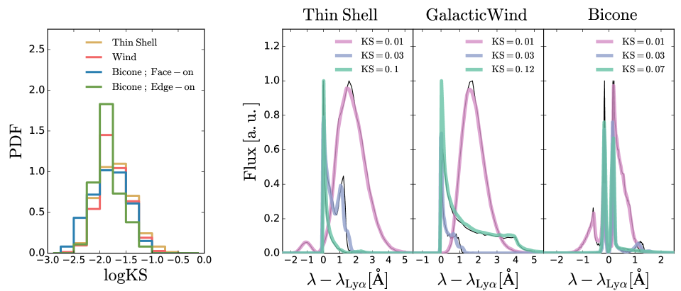
To quantify the performance of FLaREON predicting $\mathrm{Ly}\alpha$ line profiles we perform a Kolmogorov–Smirnov (KS) test over the 300 random outflow configurations for each geometry.Fig.3 shows the resulting KS distributions of the 300 random configurations for all the geometries. We find a very good agreement between the $\mathrm{Ly}\alpha$ line profiles computed by LyaRT and those predicted by FLaREON. For all geometries the KS distribution peaks around ${\rm KS}=10^{-2}$, implying that the typical maximum difference of the cumulative line profiles is $\approx 1\%$ of the flux. Additionally, about $90\%$ of the random samples exhibit ${\rm KS}<0.05$ for all geometries.

The right panels in Fig. 3 show some example geometries where the outputs of Monte Carlo LyaRT and FLaREON are compared. Overall, the differences between the Monte Carlo code and FLaREON are negligible.

Figure 5: Kolmogorov-Smirnov estimator distribution for the 1000 best fitting line profiles in different geometries. From left to right, the gas geometries used as models are: Thin shell, Galactic wind and Biconical wind. The geometries used for the fitting in each panel are the two complementary to the one used for the model. The Thin shell is shown in red, the Wind in green while the Bicone is printed in blue.

4 Hands on FLaREON

In this section we ilustrate how to execute FLaREON. After the installation, running FLaREON should only take a few Python command lines.

A simple script to compute the $\mathrm{Ly}\alpha$ escape fraction and line profiles for some given Thin shell configurations is given below:

import FLaREON as Lya, numpy as np, pylab as plt# 1) We define the configuration parameters.# 1.1) Expansion velocity in km/s :V_exp = [ 50 , 100 , 200 , 300 ]# 1.2) Logarithm of column densities in cm**-2 :log_NH= [ 18 , 19 , 20 , 21 ]# 1.3) Dust optical depths :tau_a  = [ 0.5 , 0.1 , 0.05 , 0.01 ]# 1.4) Select a geometry :Geometry = ’Thin_Shell’# 2) Compute the escape fractions.f_esc = Lya.RT_f_esc( Geometry, V_exp ,                      log_NH  , tau_a )# 3) Compute the line profiles.# 3.1) Define the wavelength range in meters.wavelength = np.linspace( 1213e-10, 1224e-10, 1000 )# 3.2) Execute FLaREONlines = Lya.RT_Line_Profile( Geometry, wavelength,                             V_exp   , log_NH    ,                             tau_a               )# 4) Display the line profiles.for line in lines :    plt.plot( wavelength , line )plt.show()

Other examples can be found in the GitHub repository, including the coupling of FLaREON with other popular public codes such as emcee (Foreman-Mackey et al., 2013) to perform $\mathrm{Ly}\alpha$ line fitting.

Figure 6: Comparison of the randomly selected model’s $\mathrm{Ly}\alpha$ line profiles and the best fitting outflow configurations using different gas geometries. The Thin shell, Galactic wind and Bicone are shown in red, green and blue respectively. Additionally line profile used as model is highlighted by thicker lines. The model outflow geometry changes from Thin shell, to Galactic wind to Bicone from left to right.

5 Some applications

In this section we present a small glimpse of the potential scientific applications of FLaREON.

5.1 Line profile properties

Recently, Verhamme et al. (2018) characterized the $\mathrm{Ly}\alpha$ line profiles to infer their displacement redwards of the line centre, allowing to infer the systemic redshift of a source from the $\mathrm{Ly}\alpha$ line only. This is done by measuring the difference in wavelength between different peaks, if there is more than one, or by measuring the FWHM of a single peak.

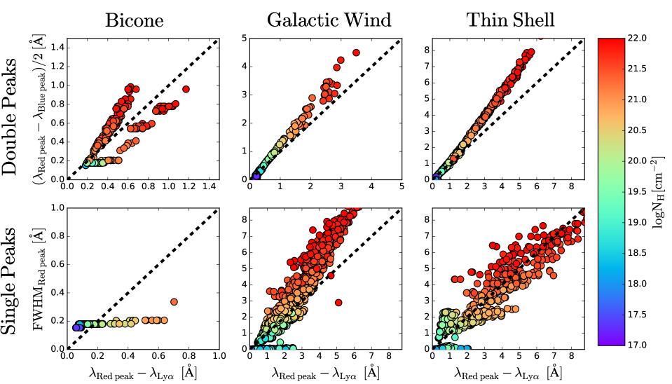
Fig. 4 shows the relation between different line profile properties for 1000 different configurations spanning the full $V_{\rm exp}-N_{\rm H}-\tau_{\rm a}$ space using the three geometries. In the top panels we show the relation between the red peak shift and half of the distance between the red and blue peak in only configurations exhibiting both peaks. In general, FLaREON predicts a tight correlation between these properties and the neutral hydrogen column density. We find that FLaREON reproduce the correlation found by Verhamme et al. (2018) for shift of the read peak smaller than 2Å where trend leaves the one-to-one relation and the slope increases.

In the bottom panels of Fig.4 we show the relation of the shift and the FWHM of the red peak in configurations where only the red peak was found. Overall, FLaREON also predicts a correlation between these properties and the column density, although with a greater scatter. Our results with FLaREON are consistent with the findings of Verhamme et al. (2018) for the Thin shell and Galactic wind geometry.

Table 1: Description of randomly selected configurations (models) and their best fitting configuration in other outflow geometries.

Configurations	$V_{\rm exp}$	$\log\;N_{\rm H}$	$\rm\log\;\tau_{a}$	$\rm log\;KS$	$f_{\rm esc}$
	$\rm[km/s]$	$\rm[cm^{-2}]$
Model   : Thin shell	55.0	17.62	-0.23	-	0.43
Best fit : Wind	62.4	17.14	-0.25	-1.5	0.58
Best fit : Bicone	890.5	17.11	-0.13	-0.5	0.46
Model   : Wind	123.0	20.25	-1.29	-	0.88
Best fit : Thin shell	93.2	20.5	-0.29	-2.2	0.07
Best fit : Bicone	616.3	22.0	-1.38	-0.6	0.8
Model   : Bicone	375.0	21.42	-2.37	-	0.97
Best fit : Thin shell	93.0	19.64	-2.75	-0.8	0.99
Best fit : Wind	348.2	19.5	-1.75	-0.7	0.98

5.2 Extract outflow information from $\mathrm{Ly}\alpha$ line profiles.

One of the most attractive application of FLaREON consists in inferring outflow properties from measured $\mathrm{Ly}\alpha$ line profiles. Usually, in this kind of analysis only one outflow geometry is implemented (e.g. Orlitová et al., 2018; Gronke, 2017). However, since FLaREON includes several gas configurations the analysis can be extended to different outflow geometries. In this section we give a glimpse of the advantages of using several geometries and we will exploit further this idea in an upcoming work (Mejias et. al., in prep).

To study how the inferred outflow properties depend on the gas geometry we start by generating a $\mathrm{Ly}\alpha$ line profile with a given gas geometry and random outflow parameters. We refer to this as model. Then, we perform an MCMC analysis combining FLaREON and emcee (Foreman-Mackey et al., 2013) with the other gas geometries to fit the line profile of the model.

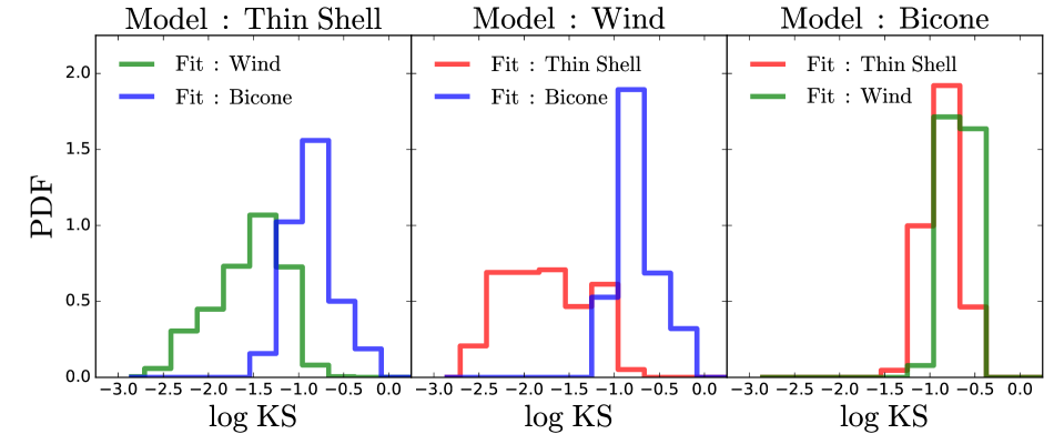
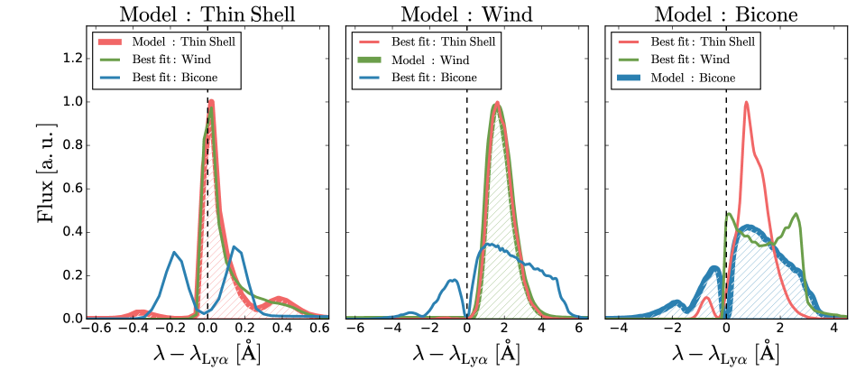
We repeat this test 1000 times per gas geometry. For the biconical geometry we use the spherically averaged configuration, but we have checked that the results resemble those obtained with the edge-on and face-on configurations. We show the Kolmogorov-Smirnov estimator distribution of the 3000 tests in Fig.5. In general, we find that the Thin shell geometry is able to produce very similar line profiles to the Galactic wind and vice verse. For both geometries we find that, when fitting the other geometry, the typical KS values fall below 0.1. In contrast we find that the line profiles produced by the biconical wind are very different from those generated by the other two geometries. In fact we find that neither of the other geometries is able to procure good fittings to the biconical geometry and vice verse. Indeed, most of the best fitting exhibit KS$>0.1$.

Additionally, we also show three detailed cases, one per gas geometry. These few examples illustrate the degeneracy between gas geometry and outflow parameters. In Fig. 6 we show a comparison between the model’s $\mathrm{Ly}\alpha$ line profile and the best fits of the other outflow geometries, whereas in Table 1 we summarize the results of the MCMC. On one hand, the morphology of the $\mathrm{Ly}\alpha$ line profiles produced by the Bicone are very different ($\rm KS>0.1$) from the line profiles generated by the Wind and Thin shell. Hence, there is not confusion between these gas geometries. On the other hand, the Thin shell and Wind line profiles resemble and fit each other $\mathrm{Ly}\alpha$ line profile with very good agreement ($\rm KS<0.1$). However, since the gas morphology impacts the resulting line profile, the inferred properties from the fit, generally, do not match the model’s characteristic.

Additionally, the $f_{\rm esc}^{\rm Ly\alpha}$ computed from the inferred outflow properties differs from the $f_{\rm esc}^{\rm Ly\alpha}$ of the model. This increases the difficulty of calculating the intrinsic $\mathrm{Ly}\alpha$ flux emitted before the radiative transfer processes by using only $\mathrm{Ly}\alpha$ emission.

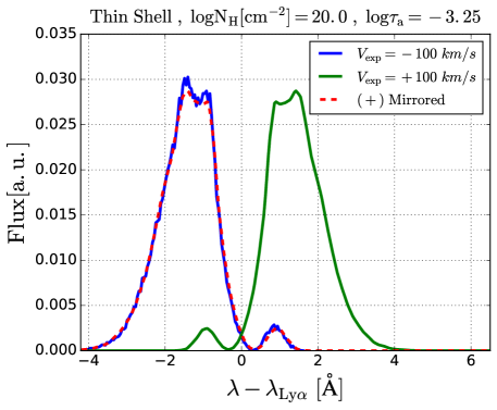
In a similar fashion, FLaREON can also be used to extract information from inflows. The $\mathrm{Ly}\alpha$ line profile emerging from an inflow with a given set of properties (gas topology, $N_{\rm H}$, $\tau_{\rm a}$ and $V_{\rm exp}<0$) can be directly computed from the outputs of FLaREON. Indeed, it is as simple as i) computing the emerging line profile of an outflow with the same gas geometry and set of properties {$N_{\rm H}$, $\tau$, $|V_{{\rm exp}}|$} and ii) mirroring the line profile with respect to the $\mathrm{Ly}\alpha$ wavelength, i.e., making the mapping

$$\centering\lambda-\lambda_{\rm Ly\alpha}\rightarrow-(\lambda-\lambda_{\rm Ly\alpha}).\@add@centering$$ (10)

In order to validate this procedure we have run LyaRT in several configurations with $\rm V_{exp}<0$. Then, for the same gas geometry, $\rm\log N_{H}$, $\rm\log\tau_{a}$ and $\rm|V_{exp}|$, we generate $\mathrm{Ly}\alpha$ line profiles with FLaREON and we apply the methodology explained above to them. In Fig.7 we show a comparison between the proper calculation of the $\mathrm{Ly}\alpha$ line profile emerging from an inflow configuration using LyaRT and the outputs of FLaREON . After the wavelength remapping, the output of FLaREON reproduces very well the full RT calculation. We have checked that this procedure works over the full parameter space exploredby FLaREON.

Figure 7: Comparison between the proper calculation of a $\mathrm{Ly}\alpha$ line profile emerging from an inflow configuration using LyaRT and the outputs of FLaREON. This example was built with the Thin shell as gas geometry, $\log N_{\rm H}{\rm[cm^{-2}]}=20$, $\rm\log\tau_{\rm a}=-3.25$ and ${|V_{\rm exp}|=100}\ {\rm km/s}$. In blue we show the full RT computation by LyaRT using ${V_{\rm exp}=-100}\ {\rm km/s}$. In green we show the FLaREON’s prediction using ${V_{\rm exp}=+100}\ {\rm km/s}$. In dashed red we show FLaREON’s output after the remapping of the wavelength (Eq.10).

6 Conclusions

In this work we have introduced FLaREON, a user-friendly public Python code based on the radiative transfer Monte Carlo code LyaRT (Orsi et al., 2012). This code is able to predict $\mathrm{Ly}\alpha$ line profiles and $\mathrm{Ly}\alpha$ escape fractions for different outflow geometries in a wide range of outflow properties without the need to run a Monte Carlo code.

FLaREON includes three different outflow geometries, an expanding Thin shell (e.g. Verhamme et al., 2006; Orsi et al., 2012; Gurung-López et al., 2019b), Galactic wind (Orsi et al., 2012; Gurung-López et al., 2019b), and a biconical outflow surrounded by a very thick static torus.

In order to predict the $\mathrm{Ly}\alpha$ line profile and $f_{\rm esc}^{\rm Ly\alpha}$  FLaREON interpolates or makes use of machine learning algorithms over previously-computed grids of configurations. This grids are very dense and cover a wide range of $\rm V_{exp}$, $\rm N_{H}$ and $\tau_{a}$. These are composed by 4704 and 12348 different outflow configurations to predict the $f_{\rm esc}^{\rm Ly\alpha}$ and line profile, respectively.

We have analyzed the performance of FLaREON of the different geometries and predicting method implemented. FLaREON is able to predict thousands of $f_{\rm esc}^{\rm Ly\alpha}$and line profiles with remarkably high accuracy. The error in $f_{\rm esc}^{\rm Ly\alpha}$ is typically below $5\%$. Additionally, the Kolmogorov-Smirnov test delivers values about 0.01 between the fully computed LyaRT line profiles and FLaREON predictions.

In future works we plan to exploit the FLaREON capabilities to predict thousands of line profiles and escape fractions to extract outflow physical information such as $V_{\rm exp}$ or $N_{\rm H}$ from observed spectra and to populate large cosmological volumes with $\mathrm{Ly}\alpha$ emitters (see Gurung-Lopez et al., 2019a).

References

- Ahn (2003) Ahn S., 2003, Journal of Korean Astronomical Society, 36, 145
- Ahn (2004) Ahn S., 2004, ApJ, 601, L25
- Ahn et al. (2000) Ahn S.-H., Lee H.-W., Lee H. M., 2000, Journal of Korean Astronomical Society, 33, 29
- Dijkstra (2017) Dijkstra M., 2017, preprint, (arXiv:1704.03416)
- Dijkstra et al. (2006) Dijkstra M., Haiman Z., Spaans M., 2006, ApJ, 649, 14
- Foreman-Mackey et al. (2013) Foreman-Mackey D., Hogg D. W., Lang D., Goodman J., 2013, PASP, 125, 306
- Garel et al. (2012) Garel T., Blaizot J., Guiderdoni B., Schaerer D., Verhamme A., Hayes M., 2012, MNRAS, 422, 310
- Granato et al. (2000) Granato G. L., Lacey C. G., Silva L., Bressan A., Baugh C. M., Cole S., Frenk C. S., 2000, ApJ, 542, 710
- Gronke (2017) Gronke M., 2017, A&A, 608, A139
- Gronke et al. (2016) Gronke M., Dijkstra M., McCourt M., Oh S. P., 2016, ApJ, 833, L26
- Gurung-Lopez et al. (2019a) Gurung-Lopez S., Orsi A. A., Bonoli S., Padilla N., Lacey C. G., Baugh C. M., 2019a, arXiv e-prints,
- Gurung-López et al. (2019b) Gurung-López S., Orsi Á. A., Bonoli S., Baugh C. M., Lacey C. G., 2019b, MNRAS, 486, 1882
- Harrington (1973) Harrington J. P., 1973, MNRAS, 162, 43
- Hu et al. (1998) Hu E. M., Cowie L. L., McMahon R. G., 1998, ApJ, 502, L99+
- Konno et al. (2016) Konno A., Ouchi M., Nakajima K., Duval F., Kusakabe H., Ono Y., Shimasaku K., 2016, ApJ, 823, 20
- Laursen & Sommer-Larsen (2007) Laursen P., Sommer-Larsen J., 2007, ApJ, 657, L69
- Laursen et al. (2009) Laursen P., Razoumov A. O., Sommer-Larsen J., 2009, ApJ, 696, 853
- Malhotra & Rhoads (2002) Malhotra S., Rhoads J. E., 2002, ApJ, 565, L71
- Neufeld (1990) Neufeld D. A., 1990, ApJ, 350, 216
- Orlitová et al. (2018) Orlitová I., Verhamme A., Henry A., Scarlata C., Jaskot A., Oey M. S., Schaerer D., 2018, A&A, 616, A60
- Orsi et al. (2012) Orsi A., Lacey C. G., Baugh C. M., 2012, MNRAS, 425, 87
- Ouchi et al. (2018) Ouchi M., et al., 2018, PASJ, 70, S13
- Pedregosa et al. (2011) Pedregosa F., et al., 2011, Journal of Machine Learning Research, 12, 2825
- Rhoads et al. (2000) Rhoads J. E., Malhotra S., Dey A., Stern D., Spinrad H., Jannuzi B. T., 2000, ApJ, 545, L85
- Silva et al. (1998) Silva L., Granato G. L., Bressan A., Danese L., 1998, arXiv e-prints, pp astro–ph/9806314
- Sobral et al. (2017) Sobral D., et al., 2017, MNRAS, 466, 1242
- Steidel et al. (1996) Steidel C. C., Giavalisco M., Pettini M., Dickinson M., Adelberger K. L., 1996, ApJ, 462, L17+
- Verhamme et al. (2006) Verhamme A., Schaerer D., Maselli A., 2006, A&A, 460, 397
- Verhamme et al. (2012) Verhamme A., Dubois Y., Blaizot J., Garel T., Bacon R., Devriendt J., Guiderdoni B., Slyz A., 2012, A&A, 546, A111
- Verhamme et al. (2018) Verhamme A., et al., 2018, MNRAS, 478, L60
- Zheng & Miralda-Escudé (2002) Zheng Z., Miralda-Escudé J., 2002, ApJ, 578, 33