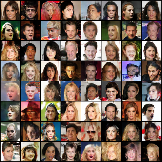
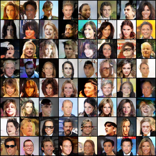
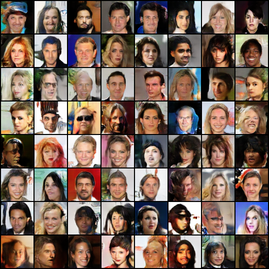
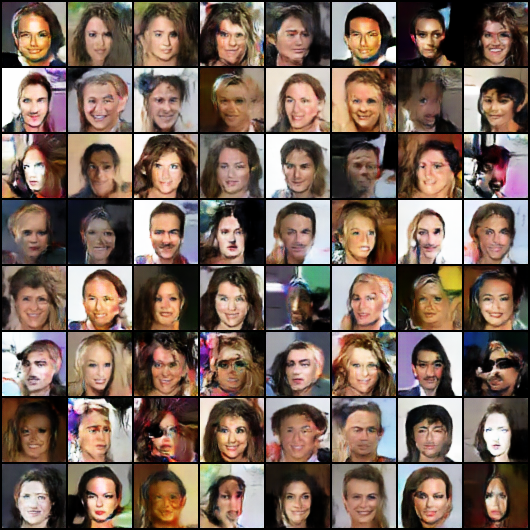
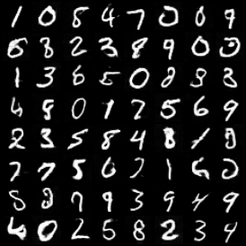
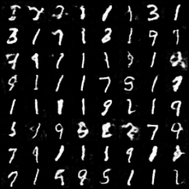
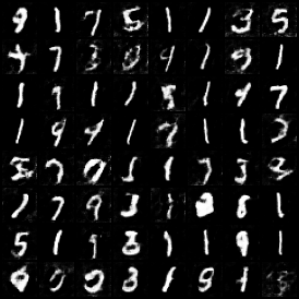
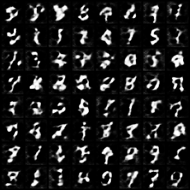
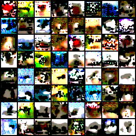
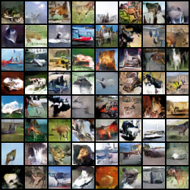
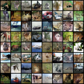
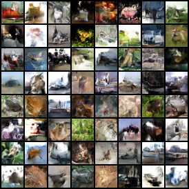
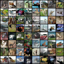
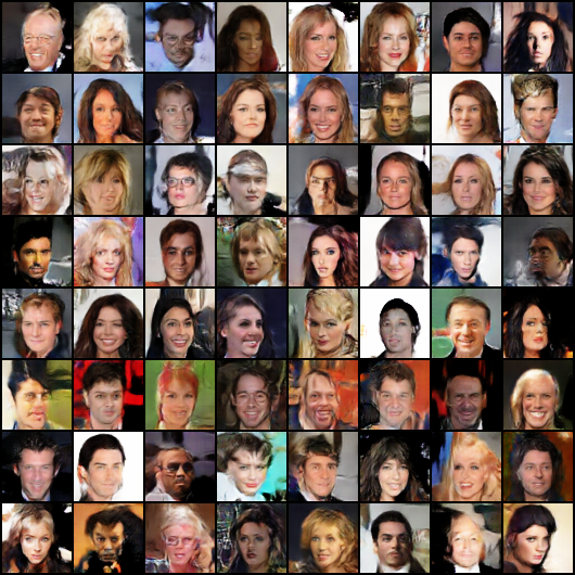
11institutetext: Cardiff University, 11email: qiny16@cardiff.ac.uk 22institutetext: UCL/Adobe Research, 22email: n.mitra@cs.ucl.ac.uk 33institutetext: KAUST, 33email: pwonka@gmail.com

How does Lipschitz Regularization
Influence GAN Training?

Yipeng Qin 1Cardiff University, 1qiny16@cardiff.ac.uk 3KAUST, 3pwonka@gmail.com    Niloy Mitra 2UCL/Adobe Research, 2n.mitra@cs.ucl.ac.uk    Peter Wonka 3KAUST, 3pwonka@gmail.com 1Cardiff University, 1qiny16@cardiff.ac.uk 3KAUST, 3pwonka@gmail.com 2UCL/Adobe Research, 2n.mitra@cs.ucl.ac.uk 3KAUST, 3pwonka@gmail.com
Abstract

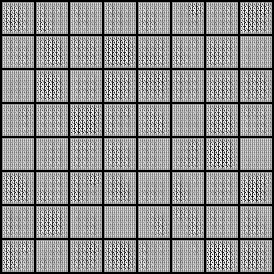
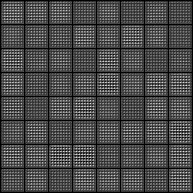
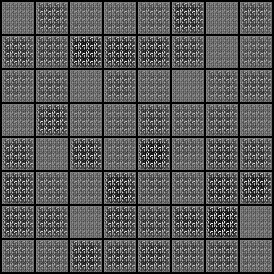
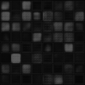
Despite the success of Lipschitz regularization in stabilizing GAN training, the exact reason of its effectiveness remains poorly understood. The direct effect of K𝐾K-Lipschitz regularization is to restrict the L2𝐿2L2-norm of the neural network gradient to be smaller than a threshold K𝐾K (e.g., K=1𝐾1K=1) such that fKnorm𝑓𝐾\|\nabla f\|\leq K. In this work, we uncover an even more important effect of Lipschitz regularization by examining its impact on the loss function: It degenerates GAN loss functions to almost linear ones by restricting their domain and interval of attainable gradient values. Our analysis shows that loss functions are only successful if they are degenerated to almost linear ones. We also show that loss functions perform poorly if they are not degenerated and that a wide range of functions can be used as loss function as long as they are sufficiently degenerated by regularization. Basically, Lipschitz regularization ensures that all loss functions effectively work in the same way. Empirically, we verify our proposition on the MNIST, CIFAR10 and CelebA datasets.

Abstract

As supplementary material to the main paper we provide the detailed network architectures (Sec. 6), additional quantitative results (Sec. 7) and additional qualitative results (Sec. 8).

Keywords:
Generative adversarial network (GAN) \cdot Lipschitz regularization \cdot loss functions

1 Introduction

Generative Adversarial Networks (GANs) are a class of generative models successfully applied to various applications, e.g., pose-guided image generation [17], image-to-image translation [29, 23], texture synthesis [5], high resolution image synthesis [27], 3D model generation [28], urban modeling [13]. Goodfellow et al. [7] proved the convergence of GAN training by assuming that the generator is always updated according to the temporarily optimal discriminator at each training step. In practice, this assumption is too difficult to satisfy and GANs remain difficult to train. To stabilize the training of the GANs, various techniques have been proposed regarding the choices of architectures [24, 10], loss functions [2, 19], regularization and normalization [2, 8, 20, 21]. We refer interested readers to [16, 14] for extensive empirical studies.

Among them, the Lipschitz regularization [8, 21] has shown great success in stabilizing the training of various GANs. For example, [18] and [4] observed that the gradient penalty Lipschitz regularizer helps to improve the training of the LS-GAN [19] and the NS-GAN [7], respectively; [21] observed that the NS-GAN, with their spectral normalization Lipschitz regularizer, works better than the WGAN [2] regularized by gradient penalty (WGAN-GP) [8].
Refer to caption
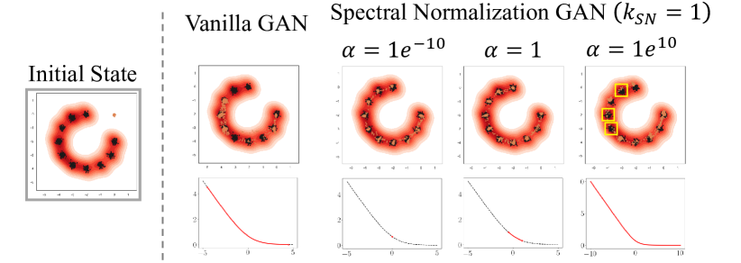
Figure 1: An illustrative 2D example. First row: model distribution (orange point) vs. data distribution (black points). Second row: domains of the loss function (red curve). It can be observed that the performance of spectral normalized GANs [21] worsen when their domains are enlarged (α=1e10𝛼1superscript𝑒10\alpha=1e^{10}, yellow boxes). However, good performance can always be achieved when their domains are restricted to near-linear ones (α=1e10𝛼1superscript𝑒10\alpha=1e^{-10} and α=1𝛼1\alpha=1). Please see Sections 3.2 and 4.1 for the definitions of α𝛼\alpha and kSNsubscript𝑘𝑆𝑁k_{SN}, respectively.
Refer to caption
Refer to caption
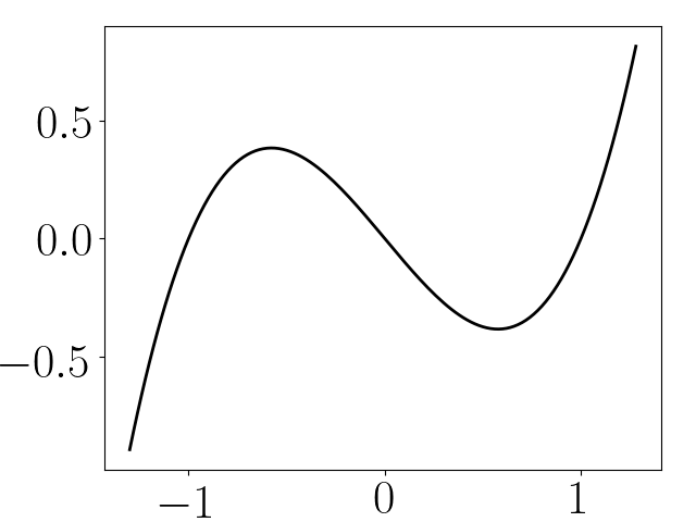
(a) f(x)=x3x𝑓𝑥superscript𝑥3𝑥f(x)=x^{3}-x
Refer to caption
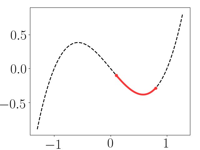
(b) [a,b]=[0.1,0.8]𝑎𝑏0.10.8[a,b]=[0.1,0.8]
Refer to caption
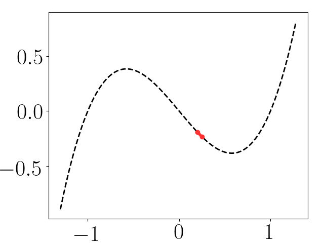
(c) [a,b]=[0.2,0.25]𝑎𝑏0.20.25[a,b]=[0.2,0.25]
Figure 2: First row: Applying Lipschitz regularization restricts the domain of the loss function to an interval Ω=[a,b]Ω𝑎𝑏\Omega=[a,b]. Second row: Illustration of the domain restriction. We take a third-order polynomial loss function f(x)=x3x𝑓𝑥superscript𝑥3𝑥f(x)=x^{3}-x as an example. Its restricted domain [a,b]𝑎𝑏[a,b] is shown in red. (a) without restriction f(x)𝑓𝑥f(x) is non-convex. (b) Restricting the domain of f(x)𝑓𝑥f(x) makes it convex. (c) f(x)𝑓𝑥f(x) is almost linear when its domain is restricted to a very small interval.

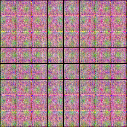
In this paper, we provide an analysis to better understand the coupling of Lipschitz regularization and the choice of loss function. Our main insight is that the rule of thumb of using small Lipschitz constants (e.g., K=1𝐾1K=1) is degenerates the loss functions to almost linear ones by restricting their domain and interval of attainable gradient values (see Figure 1). These degenerate losses improve GAN training. Because of this, the exact shapes of the loss functions before degeneration do not seem to matter that much. We demonstrate this by two experiments. First, we show that when K𝐾K is sufficiently small, even GANs trained with non-standard loss functions (e.g., cosine) give comparable results to all other loss functions. Second, we can directly degenerate loss functions by introducing domain scaling. This enables successful GAN training for a wide range of K𝐾K for all loss functions, which only worked for the Wasserstein loss before. Our contributions include:

  • We discovered an important effect of Lipschitz regularization. It restricts the domain of the loss function (Figure 2).

  • Our analysis suggests that although the choice of loss functions matters, the successful ones currently being used are all near-linear within the chosen small domains and actually work in the same way.

2 Related Work

2.1 GAN Loss Functions

A variety of GAN loss functions have been proposed from the idea of understanding the GAN training as the minimization of statistical divergences. Goodfellow et al. [7] first proposed to minimize the Jensen-Shannon (JS) divergence between the model distribution and the target distribution. In their method, the neural network output of the discriminator is first passed through a sigmoid function to be scaled into a probability in [0,1]01[0,1]. Then, the cross-entropy loss of the probability is measured. Following [4], we refer to such loss as the minimax (MM) loss since the GAN training is essentially a minimax game. However, because of the saturation at both ends of the sigmoid function, the MM loss can lead to vanishing gradients and thus fails to update the generator. To compensate for it, Goodfellow et al. [7] proposed a variant of MM loss named the non-saturating (NS) loss, which heuristically amplifies the gradients when updating the generator.

Observing that the JS divergence is a special case of the f𝑓f-divergence, Nowozin et al. [22] extended the idea of Goodfellow et al. [7] and showed that any f𝑓f-divergence can be used to train GANs. Their work suggested a new direction of improving the performance of the GANs by employing “better” divergence measures.

Following this direction, Arjovsky et al. first pointed out the flaws of the JS divergence used in GANs [1] and then proposed to use the Wasserstein distance instead (WGAN) [2]. In their implementation, the raw neural network output of the discriminator is directly used (i.e. the WGAN loss function is an identity function) instead of being passed through the sigmoid cross-entropy loss function. However, to guarantee that their loss is a valid Wasserstein distance metric, the discriminator is required to be Lipschitz continuous. Such requirement is usually fulfilled by applying an extra Lipschitz regularizer to the discriminator. Meanwhile, Mao et al. [19] proposed the Least-Square GAN (LS-GAN) to minimize the Pearson χ2superscript𝜒2\chi^{2} divergence between two distributions. In their implementation, the sigmoid cross-entropy loss is replaced by a quadratic loss.

2.2 Lipschitz Regularization

The first practice of applying the Lipschitz regularization to the discriminator came together with the WGAN [2]. While at that time, it was not employed to improve the GAN training but just a requirement of the Kantorovich-Rubinstein duality applied. In [2], the Lipschitz continuity of the discriminator is enforced by weight clipping. Its main idea is to clamp the weights of each neural network layer to a small fixed range [c,c]𝑐𝑐[-c,c], where c𝑐c is a small positive constant. Although weight clipping guarantees the Lipschitz continuity of the discriminator, the choice of parameter c𝑐c is difficult and prone to invalid gradients.

To this end, Gulrajani et al. [8] proposed the gradient penalty (GP) Lipschitz regularizer to stabilize the WGAN training, i.e. WGAN-GP. In their method, an extra regularization term of discriminator’s gradient magnitude is weighted by parameter λ𝜆\lambda and added into the loss function. In [8], the gradient penalty regularizer is one-centered, aiming at enforcing 1-Lipschitz continuity. While Mescheder et al. [20] argued that the zero-centered one should be more reasonable because it makes the GAN training converge. However, one major problem of gradient penalty is that it is computed with finite samples, which makes it intractable to be applied to the entire output space. To sidestep this problem, the authors proposed to heuristically sample from the straight lines connecting model distribution and target distribution. However, this makes their approach heavily dependent on the support of the model distribution [21].

Addressing this issue, Miyato et al. [21] proposed the spectral normalization (SN) Lipschitz regularizer which enforces the Lipschitz continuity of a neural network in the operator space. Observing that the Lipschitz constant of the entire neural network is bounded by the product of those of its layers, they break down the problem to enforcing Lipschitz regularization on each neural network layer. These simplified sub-problems can then be solved by normalizing the weight matrix of each layer according to its largest singular value.

3 Restrictions of GAN Loss Functions

In this section, first we derive why a K𝐾K-Lipschitz regularized discriminator restricts the domain and interval of attainable gradient values of the loss function to intervals bounded by K𝐾K (Section 3.1). Second, we propose a scaling method to restrict the domain of the loss function without changing K𝐾K (Section 3.2).

3.1 How does the Restriction Happen?

Let us consider a simple discriminator D(x)=L(f(x))𝐷𝑥𝐿𝑓𝑥D(x)=L(f(x)), where x𝑥x is the input, f𝑓f is a neural network with scalar output, L𝐿L is the loss function. During training, the loss function L𝐿L works by backpropagating the gradient L=L(f(x))/f(x)𝐿𝐿𝑓𝑥𝑓𝑥\nabla L=\partial L(f(x))/\partial f(x) to update the neural network weights:

D(x)Wn=𝑳(𝒇(𝒙))𝒇(𝒙)f(x)Wn𝐷𝑥superscript𝑊𝑛𝑳𝒇𝒙𝒇𝒙𝑓𝑥superscript𝑊𝑛\frac{\partial D(x)}{\partial W^{n}}=\bm{\frac{\partial L(f(x))}{\partial f(x)}}\frac{\partial f(x)}{\partial W^{n}} (1)

where Wnsuperscript𝑊𝑛W^{n} is the weight matrix of the n𝑛n-th layer. Let X𝑋X and ΩΩ\Omega be the domain and the range of f𝑓f respectively (i.e., f:XΩ:𝑓𝑋Ωf:X\to\Omega), it can be easily derived that the attainable values of L𝐿\nabla L is determined by ΩΩ\Omega (i.e., L:ΩΨ:𝐿ΩΨ\nabla L:\Omega\to\Psi). Without loss of generality, we assume that xX=[1,1]m×n×3𝑥𝑋superscript11𝑚𝑛3x\in X=[-1,1]^{m\times n\times 3} are normalized images and derive the bound of the size of ΩΩ\Omega as follows:

Theorem 3.1

If the discriminator neural network f𝑓f satisfies the k𝑘k-Lipschitz continuity condition, we have f:XΩ:𝑓𝑋Ωf:X\to\Omega\subset\mathbb{R} satisfying |min(Ω)max(Ω)|k12mnΩΩ𝑘12𝑚𝑛|\min(\Omega)-\max(\Omega)|\leq k\sqrt{12mn}.

Proof

Given a k𝑘k-Lipschitz continuous neural newtork f𝑓f, for all x1,x2Xsubscript𝑥1subscript𝑥2𝑋x_{1},x_{2}\in X, we have:

|f(x1)f(x2)|kx1x2.𝑓subscript𝑥1𝑓subscript𝑥2𝑘normsubscript𝑥1subscript𝑥2|f(x_{1})-f(x_{2})|\leq k\|x_{1}-x_{2}\|. (2)

Let xb,xwXsubscript𝑥𝑏subscript𝑥𝑤𝑋x_{b},x_{w}\in X be the pure black and pure white images that maximize the Euclidean distance:

xbxw=(11)2mn3=12mn.normsubscript𝑥𝑏subscript𝑥𝑤superscript112𝑚𝑛312𝑚𝑛\|x_{b}-x_{w}\|=\sqrt{(-1-1)^{2}\cdot m\cdot n\cdot 3}=\sqrt{12mn}. (3)

Thus, we have:

|f(x1)f(x2)|kx1x2kxbxw=k12mn.𝑓subscript𝑥1𝑓subscript𝑥2𝑘delimited-∥∥subscript𝑥1subscript𝑥2𝑘delimited-∥∥subscript𝑥𝑏subscript𝑥𝑤𝑘12𝑚𝑛\begin{split}|f(x_{1})-f(x_{2})|&\leq k\|x_{1}-x_{2}\|\\ &\leq k\|x_{b}-x_{w}\|=k\sqrt{12mn}.\end{split} (4)

Thus, the range of f𝑓f is restricted to ΩΩ\Omega, which satisfies:

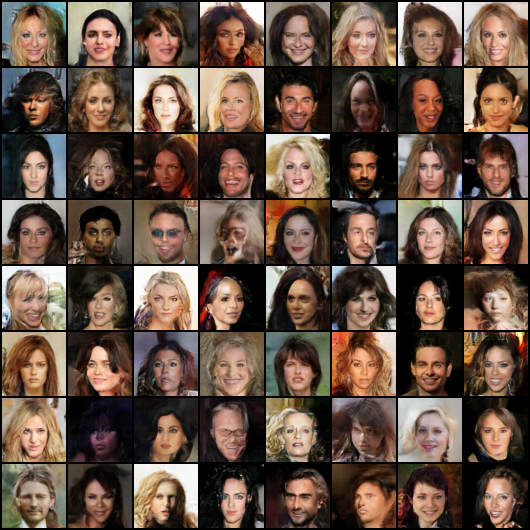
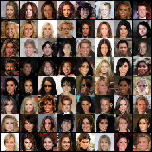
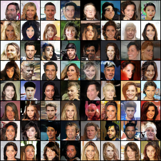
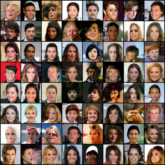
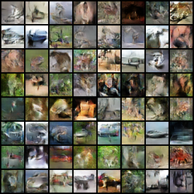
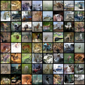
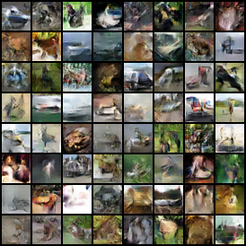
|min(Ω)max(Ω)|k12mnΩΩ𝑘12𝑚𝑛|\min(\Omega)-\max(\Omega)|\leq k\sqrt{12mn} (5)

Theorem 3.1 shows that the size of ΩΩ\Omega is bounded by k𝑘k. However, k𝑘k can be unbounded when Lipschitz regularization is not enforced during training, which results in an unbounded ΩΩ\Omega and a large interval of attainable gradient values. On the contrary, when K𝐾K-Lipschitz regularization is applied (i.e., kK𝑘𝐾k\leq K), the loss function L𝐿L is restricted as follows:

Corollary 1 (Restriction of Loss Function)

Assume that f𝑓f is a Lipschitz regularized neural network whose Lipschitz constant kK𝑘𝐾k\leq K, the loss function L𝐿L is C2superscript𝐶2C^{2}-continuous with M𝑀M as the maximum absolute value of its second derivatives in its domain. Let ΨΨ\Psi be the interval of attainable gradient values that L:ΩΨ:𝐿ΩΨ\nabla L:\Omega\to\Psi, we have

|min(Ω)max(Ω)|K12mnΩΩ𝐾12𝑚𝑛\big{|}\min(\Omega)-\max(\Omega)\big{|}\leq K\sqrt{12mn} (6)
|min(Ψ)max(Ψ)|MK12mnΨΨ𝑀𝐾12𝑚𝑛\big{|}\min(\Psi)-\max(\Psi)\big{|}\leq M\cdot K\sqrt{12mn} (7)

Corollary 7 shows that under a mild condition (C2superscript𝐶2C^{2}-continuous), applying K𝐾K-Lipschitz regularization restricts the domain ΩΩ\Omega and thereby the interval of attainable gradient values ΨΨ\Psi of the loss function L𝐿L to intervals bounded by K𝐾K. When K𝐾K is small, e.g., K=1𝐾1K=1 [8, 4, 18, 21], the interval of attainable gradient values of the loss function is considerably reduced, which prevents the backpropagation of vanishing or exploding gradients and thereby stabilizes the training. Empirically, we will show that these restrictions are indeed significant in practice and strongly influence the training.
Refer to caption
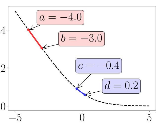
Figure 3: Domain [a,b]𝑎𝑏[a,b] shifts to [c,d]𝑐𝑑[c,d].

Change in ΩisubscriptΩ𝑖\Omega_{i} During Training. So far we analyzed the restriction of the loss function by a static discriminator. However, the discriminator neural network f𝑓f is dynamically updated during training and thus its range Ω=iΩisuperscriptΩsubscript𝑖subscriptΩ𝑖\Omega^{\cup}=\cup_{i}\Omega_{i}, where ΩisubscriptΩ𝑖\Omega_{i} is the discriminator range at each training step i𝑖i. Therefore, we need to analyze two questions:
(i) How does the size of ΩisubscriptΩ𝑖\Omega_{i} change during training?
(ii) Does ΩisubscriptΩ𝑖\Omega_{i} shift during training (Figure 3)?

For question (i), the size of ΩisubscriptΩ𝑖\Omega_{i} is always bounded by the Lipschitz constant K𝐾K throughout the training (Corollary 7). For question (ii), the answer depends on the discriminator loss function:

  • The shifting of ΩisubscriptΩ𝑖\Omega_{i} is prevented if the loss function is strictly convex. For example, the discriminator loss function of NS-GAN [7] (Table 1) is strictly convex and has a unique minimum when f(x)=f(g(z))=0𝑓𝑥𝑓𝑔𝑧0f(x)=f(g(z))=0 at convergence. Thus, minimizing it forces ΩisubscriptΩ𝑖\Omega_{i} to be positioned around 00 and prevents it from shifting. The discriminator loss function of LS-GAN [19] (Table 1) has a similar behavior. Its ΩisubscriptΩ𝑖\Omega_{i} is positioned around 0.50.50.5, since its minimum is achieved when f(x)=f(g(z))=0.5𝑓𝑥𝑓𝑔𝑧0.5f(x)=f(g(z))=0.5 at convergence. In this scenario, the ΩisubscriptΩ𝑖\Omega_{i} is relatively fixed throughout the training. Thus, ΩsuperscriptΩ\Omega^{\cup} is still roughly bounded by the Lipschitz constant K𝐾K.

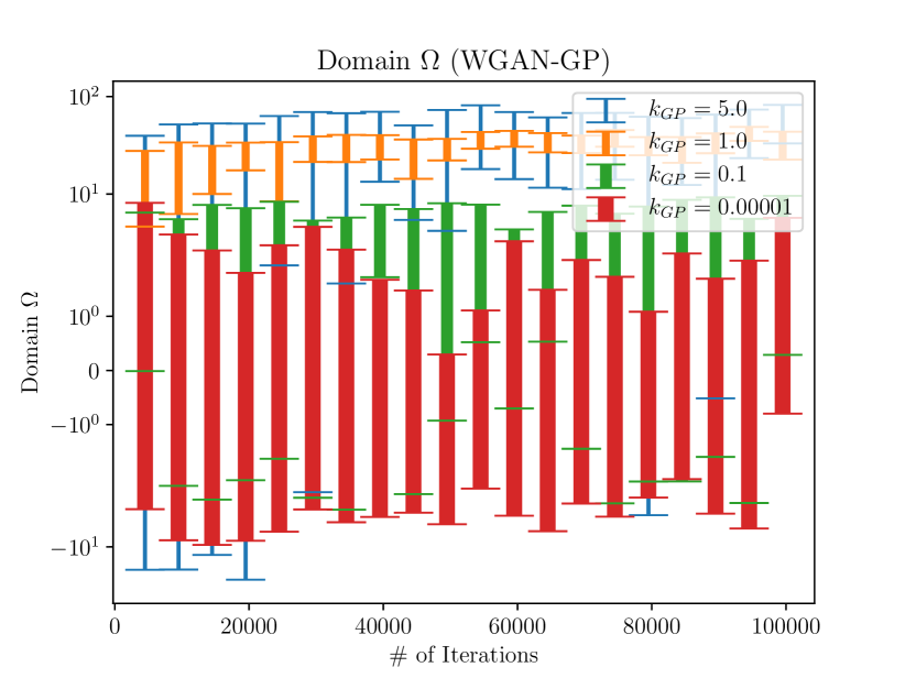
  • When the discriminator loss functions is not strictly convex, ΩisubscriptΩ𝑖\Omega_{i} may be allowed to shift. For example, the WGAN [2] discriminator loss function (Table 1) is linear and achieves its minimum when f(x)=f(g(z))𝑓𝑥𝑓𝑔𝑧f(x)=f(g(z)) at convergence. Thus, it does not enforce the domain ΩisubscriptΩ𝑖\Omega_{i} to be fixed. However, the linear WGAN loss function has a constant gradient that is independent of ΩisubscriptΩ𝑖\Omega_{i}. Thus, regarding to the interval of attainable gradient values (Eq.7), we can view it as a degenerate loss function that still fits in our discussion. Interestingly, we empirically observed that the domain ΩisubscriptΩ𝑖\Omega_{i} of WGANs also get relatively fixed at late stages of the training (Figure 4).

Table 1: The GAN loss functions used in our experiments. f()𝑓f(\cdot) is the output of the discriminator neural network; g()𝑔g(\cdot) is the output of the generator; x𝑥x is a sample from the training dataset; z𝑧z is a sample from the noise distribution. LS-GAN# is the zero-centered version of LS-GAN [18], and for the NS-GAN, f()=sigmoid[f()]superscript𝑓sigmoiddelimited-[]𝑓f^{*}(\cdot)=\mathrm{sigmoid}[f(\cdot)]. The figure on the right shows the shape of the loss functions at different scales. The dashed lines show non-standard loss functions: cos\cos and exp\exp.
GAN types Discriminator Loss Generator Loss
NS-GAN LD=𝔼[log(f(x))]𝔼[log(1f(g(z)))]subscript𝐿𝐷𝔼delimited-[]superscript𝑓𝑥𝔼delimited-[]1superscript𝑓𝑔𝑧L_{D}=-\mathbb{E}[\log(f^{*}(x))]-\mathbb{E}[\log(1-f^{*}(g(z)))] LG=𝔼[log(f(g(z)))]subscript𝐿𝐺𝔼delimited-[]superscript𝑓𝑔𝑧L_{G}=-\mathbb{E}[\log(f^{*}(g(z)))]
LS-GAN LD=𝔼[(f(x)1)2]+𝔼[f(g(z))2]subscript𝐿𝐷𝔼delimited-[]superscript𝑓𝑥12𝔼delimited-[]𝑓superscript𝑔𝑧2L_{D}=\mathbb{E}[(f(x)-1)^{2}]+\mathbb{E}[f(g(z))^{2}] LG=𝔼[(f(g(z))1)2]subscript𝐿𝐺𝔼delimited-[]superscript𝑓𝑔𝑧12L_{G}=\mathbb{E}[(f(g(z))-1)^{2}]
LS-GAN# LD=𝔼[(f(x)1)2]+𝔼[(f(g(z))+1)2]subscript𝐿𝐷𝔼delimited-[]superscript𝑓𝑥12𝔼delimited-[]superscript𝑓𝑔𝑧12L_{D}=\mathbb{E}[(f(x)-1)^{2}]+\mathbb{E}[(f(g(z))+1)^{2}] LG=𝔼[(f(g(z))1)2]subscript𝐿𝐺𝔼delimited-[]superscript𝑓𝑔𝑧12L_{G}=\mathbb{E}[(f(g(z))-1)^{2}]
WGAN LD=𝔼[f(x)]𝔼[f(g(z))]subscript𝐿𝐷𝔼delimited-[]𝑓𝑥𝔼delimited-[]𝑓𝑔𝑧L_{D}=\mathbb{E}[f(x)]-\mathbb{E}[f(g(z))] LG=𝔼[f(g(z))]subscript𝐿𝐺𝔼delimited-[]𝑓𝑔𝑧L_{G}=\mathbb{E}[f(g(z))]
COS-GAN LD=𝔼[cos(f(x)1)]𝔼[cos(f(g(z))+1)]subscript𝐿𝐷𝔼delimited-[]𝑓𝑥1𝔼delimited-[]𝑓𝑔𝑧1L_{D}=-\mathbb{E}[\cos(f(x)-1)]-\mathbb{E}[\cos(f(g(z))+1)] LG=𝔼[cos(f(g(z))1)]subscript𝐿𝐺𝔼delimited-[]𝑓𝑔𝑧1L_{G}=-\mathbb{E}[\cos(f(g(z))-1)]
EXP-GAN LD=𝔼[exp(f(x))]+𝔼[exp(f(g(z)))]subscript𝐿𝐷𝔼delimited-[]𝑓𝑥𝔼delimited-[]𝑓𝑔𝑧L_{D}=\mathbb{E}[\exp(f(x))]+\mathbb{E}[\exp(-f(g(z)))] LG=𝔼[exp(f(g(z)))]subscript𝐿𝐺𝔼delimited-[]𝑓𝑔𝑧L_{G}=\mathbb{E}[\exp(f(g(z)))]
[Uncaptioned image]

3.2 Restricting Loss Functions by Domain Scaling

As discussed above, applying K𝐾K-Lipschitz regularization not only restricts the gradients of the discriminator, but as a side effect also restricts the domain of the loss function to an interval ΩΩ\Omega. However, we would like to investigate these two effects separately. To this end, we propose to decouple the restriction of ΩΩ\Omega from the Lipschitz regularization by scaling the domain of loss function L𝐿L by a positive constant α𝛼\alpha as follows,

Lα(Ω)=L(αΩ)/α.subscript𝐿𝛼Ω𝐿𝛼Ω𝛼L_{\alpha}(\Omega)={L(\alpha\cdot\Omega)}/{\alpha}. (8)

Note that the α𝛼\alpha in the denominator helps to preserve the gradient scale of the loss function. With this scaling method, we can effectively restrict L𝐿L to an interval αΩ𝛼Ω\alpha\cdot\Omega without adjusting K𝐾K.

Degenerate Loss Functions. To explain why this works, we observe that any loss function degenerates as its domain ΩΩ\Omega shrinks to a single value. According to Taylor’s expansion, let ω,ω+ΔωΩ𝜔𝜔Δ𝜔Ω\omega,\omega+\Delta\omega\in\Omega, we have:

L(ω+Δω)=L(ω)+L(ω)1!Δω+L′′(ω)2!(Δω)2+.𝐿𝜔Δ𝜔𝐿𝜔superscript𝐿𝜔1Δ𝜔superscript𝐿′′𝜔2superscriptΔ𝜔2L(\omega+\Delta\omega)=L(\omega)+\frac{L^{\prime}(\omega)}{1!}\Delta\omega+\frac{L^{\prime\prime}(\omega)}{2!}(\Delta\omega)^{2}+\cdots. (9)

As |max(Ω)min(Ω)|ΩΩ|\max(\Omega)-\min(\Omega)| shrinks to zero, we have L(ω+Δω)L(ω)+L(ω)Δω𝐿𝜔Δ𝜔𝐿𝜔superscript𝐿𝜔Δ𝜔L(\omega+\Delta\omega)\approx L(\omega)+L^{\prime}(\omega)\Delta\omega showing that we can approximate any loss function by a linear function with constant gradient as its domain ΩΩ\Omega shrinks to a single value. Let ωΩ𝜔Ω\omega\in\Omega, we implement the degeneration of a loss function by scaling its domain ΩΩ\Omega with an extremely small constant α𝛼\alpha:

limα0Lα(ω)ω=1αL(αω)ω=L(αω)(αω)=L(0).subscript𝛼0subscript𝐿𝛼𝜔𝜔1𝛼𝐿𝛼𝜔𝜔𝐿𝛼𝜔𝛼𝜔𝐿0\lim_{\alpha\to 0}\frac{\partial L_{\alpha}(\omega)}{\partial\omega}=\frac{1}{\alpha}\cdot\frac{\partial L(\alpha\cdot\omega)}{\partial\omega}=\frac{\partial L(\alpha\cdot\omega)}{\partial(\alpha\cdot\omega)}=\nabla L(0). (10)

In our work, we use α=1e25𝛼1superscript𝑒25\alpha=1e^{-25}, smaller values are not used due to numerical errors (NaN𝑁𝑎𝑁NaN).

4 Experiments

To support our proposition, first we empirically verify that applying K𝐾K-Lipschitz regularization to the discriminator has the side-effect of restricting the domain and interval of attainable gradient values of the loss function. Second, with the proposed scaling method (Section 3.2), we investigate how the varying restrictions of loss functions influence the performance of GANs when the discriminator is regularized with a fixed Lipschitz constant. Third, we show that restricting the domain of any loss function (using decreasing α𝛼\alpha) converges to the same (or very similar) performance as WGAN-SN.

4.1 Experiment Setup

General Setup. In the following experiments, we use two variants of the standard CNN architecture [24, 2, 21] for the GANs to learn the distributions of the MNIST, CIFAR10 datasets at 32×32323232\times 32 resolution and the CelebA dataset [15] at 64×64646464\times 64 resolution. Details of the architectures are shown in the supplementary material. We use a batch size of 646464 to train the GANs. Similar to [2], we observed that the training could be unstable with a momentum-based optimizer such as Adam, when the discriminator is regularized with a very small Lipschitz constant K𝐾K. Thus, we choose to use an RMSProp optimizer with learning rate 0.000050.000050.00005. To make a fair comparison, we fix the number of discriminator updates in each iteration ndis=1subscript𝑛𝑑𝑖𝑠1n_{dis}=1 for all the GANs tested (i.e., we do not use multiple discriminator updates like [1, 2]). Unless specified, we stop the training after 105superscript10510^{5} iterations.

Refer to caption
(a)
Refer to caption
(b)
Refer to caption
(c)
Refer to caption
(d)
Refer to caption
(e)
Refer to caption
(f)
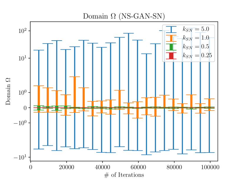
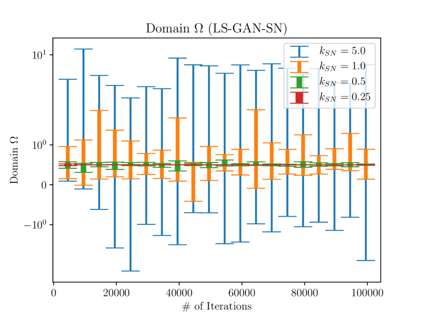
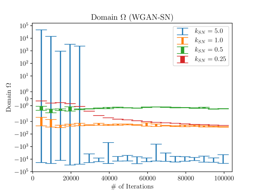
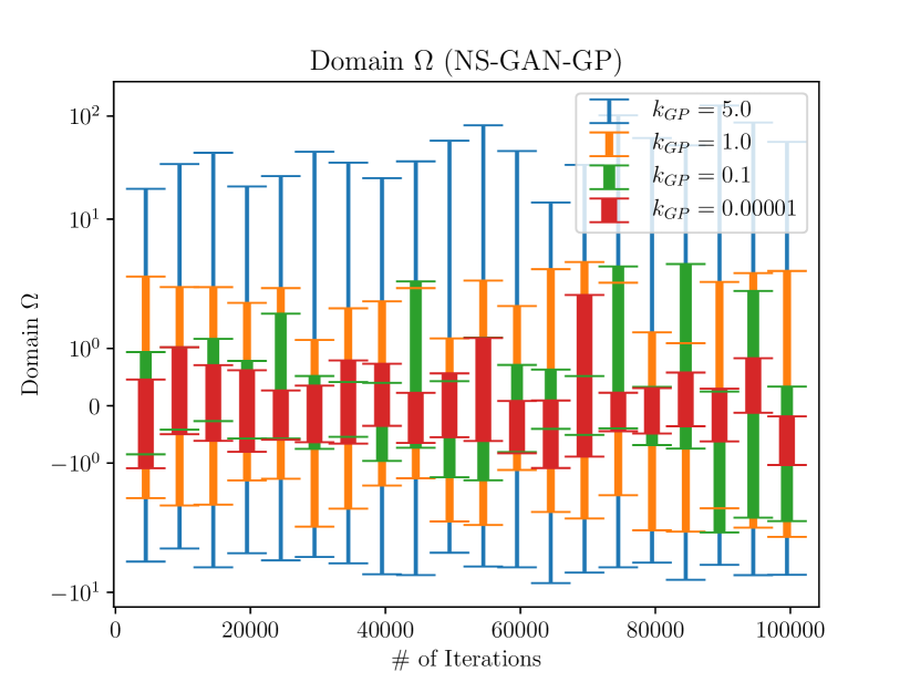
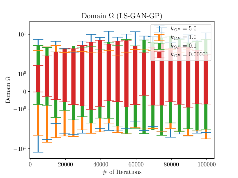
Figure 4: Relationship between domain ΩΩ\Omega and kGPsubscript𝑘𝐺𝑃k_{GP}, kSNsubscript𝑘𝑆𝑁k_{SN} for different loss functions on CelebA dataset, where kGPsubscript𝑘𝐺𝑃k_{GP}, kSNsubscript𝑘𝑆𝑁k_{SN} are the parameters controlling the strength of the Lipschitz regularizers. The domain ΩΩ\Omega shrinks with decreasing kGPsubscript𝑘𝐺𝑃k_{GP} or kSNsubscript𝑘𝑆𝑁k_{SN}. Each column shares the same loss function while each row shares the same Lipschitz regularizer. NS-GAN: Non-Saturating GAN [7]; LS-GAN: Least-Square GAN [19]; WGAN: Wasserstein GAN [2]; GP: gradient penalty [8]; SN: spectral normalization [21]. Note that the y𝑦y-axis is in log\log scale.

Lipschitz Regularizers. In general, there are two state-of-the-art Lipschitz regularizers: the gradient penalty (GP) [8] and the spectral normalization (SN) [21]. In their original settings, both techniques applied only 111-Lipschitz regularization to the discriminator. However, our experiments require altering the Lipschitz constant K𝐾K of the discriminator. To this end, we propose to control K𝐾K for both techniques by adding parameters kGPsubscript𝑘𝐺𝑃k_{GP} and kSNsubscript𝑘𝑆𝑁k_{SN}, respectively.

  • For the gradient penalty, we control its strength by adjusting the target gradient norm kGPsubscript𝑘𝐺𝑃k_{GP},

    L=LGAN+λ𝔼x^Px^[(x^D(x^)kGP)2],𝐿subscript𝐿𝐺𝐴𝑁𝜆subscript𝔼^𝑥subscript𝑃^𝑥delimited-[]superscriptnormsubscript^𝑥𝐷^𝑥subscript𝑘𝐺𝑃2L=L_{GAN}+\lambda\mathop{\mathbb{E}}_{\hat{x}\in P_{\hat{x}}}[(\|\bigtriangledown_{\hat{x}}D(\hat{x})\|-k_{GP})^{2}], (11)

    where LGANsubscript𝐿𝐺𝐴𝑁L_{GAN} is the GAN loss function without gradient penalty, λ𝜆\lambda is the weight of the gradient penalty term, Px^subscript𝑃^𝑥P_{\hat{x}} is the distribution of linearly interpolated samples between the target distribution and the model distribution [8]. Similar to [8, 4], we use λ=10𝜆10\lambda=10.

  • For the spectral normalization, we control its strength by adding a weight parameter kSNsubscript𝑘𝑆𝑁k_{SN} to the normalization of each neural network layer,

    W¯SN(W,kSN):=kSNW/σ(W),assignsubscript¯𝑊𝑆𝑁𝑊subscript𝑘𝑆𝑁subscript𝑘𝑆𝑁𝑊𝜎𝑊\bar{W}_{SN}(W,k_{SN}):=k_{SN}\cdot W/\sigma(W), (12)

    where W𝑊W is the weight matrix of each layer, σ(W)𝜎𝑊\sigma(W) is its largest singular value.

The relationship between kSNsubscript𝑘𝑆𝑁k_{SN} and K𝐾K can be quantitatively approximated as KkSNn𝐾superscriptsubscript𝑘𝑆𝑁𝑛K\approx k_{SN}^{n} [21], where n𝑛n is the number of neural network layers in the discriminator. While for kGPsubscript𝑘𝐺𝑃k_{GP}, we can only describe its relationship against K𝐾K qualitatively as: the smaller kGPsubscript𝑘𝐺𝑃k_{GP}, the smaller K𝐾K. The challenge on finding a quantitative approximation resides in that the gradient penalty term λ𝔼x^Px^[(x^D(x^)kGP)2]𝜆subscript𝔼^𝑥subscript𝑃^𝑥delimited-[]superscriptnormsubscript^𝑥𝐷^𝑥subscript𝑘𝐺𝑃2\lambda\mathop{\mathbb{E}}_{\hat{x}\in P_{\hat{x}}}[(\|\bigtriangledown_{\hat{x}}D(\hat{x})\|-k_{GP})^{2}] has no upper bound during training (Eq.11). We also verified our claims using Stable Rank Normalization (SRN)+SN [25] as the Lipschitz regularizer, whose results are shown in the supplementary material.

Loss Functions. In Table 1 we compare the three most widely-used GAN loss functions: the Non-Saturating (NS) loss function [7], the Least-Squares (LS) loss function [19] and the Wasserstein loss function [2]. In addition, we also test the performance of the GANs using some non-standard loss functions, cos()\cos(\cdot) and exp()\exp(\cdot), to support the observation that the restriction of the loss function is the dominating factor of Lipschitz regularization. Note that both the cos()\cos(\cdot) and exp()\exp(\cdot) loss functions are (locally) convex at convergence, which helps to prevent shifting ΩisubscriptΩ𝑖\Omega_{i} (Section 3.1).

Quantitative Metrics. To quantitatively measure the performance of the GANs, we follow the best practice and employ the Fréchet Inception Distance (FID) metric [11] in our experiments. The smaller the FID score, the better the performance of the GAN. The results on other metrics, i.e. Inception scores [3] and Neural Divergence [9], are shown in the supplementary material.

4.2 Empirical Analysis of Lipschitz Regularization

In this section, we empirically analyze how varying the strength of the Lipschitz regularization impacts the domain, interval of attained gradient values, and performance (FID scores) of different loss functions (Section 3.1).

Domain vs. Lipschitz Regularization. In this experiment, we show how the Lipschitz regularization influences the domain of the loss function. As Figure 4 shows, we plot the domain ΩΩ\Omega as intervals for different iterations under different kGPsubscript𝑘𝐺𝑃k_{GP} and kSNsubscript𝑘𝑆𝑁k_{SN} for the gradient penalty and the spectral normalization regularizers respectively. It can be observed that: (i) For both regularizers, the interval ΩΩ\Omega shrinks as kGPsubscript𝑘𝐺𝑃k_{GP} and kSNsubscript𝑘𝑆𝑁k_{SN} decreases. However, kSNsubscript𝑘𝑆𝑁k_{SN} is much more impactful than kGPsubscript𝑘𝐺𝑃k_{GP} in restricting ΩΩ\Omega. Thus, we use spectral normalization to alter the strength of the Lipschitz regularization in the following experiments. (ii) For NS-GANs and LS-GANs, the domains ΩisubscriptΩ𝑖\Omega_{i} are rather fixed during training. For WGANs, the domains ΩisubscriptΩ𝑖\Omega_{i} typically shift at the beginning of the training, but then get relatively fixed in later stages.

Table 2: Domain ΩΩ\Omega and the interval of attained gradient values L(Ω)𝐿Ω\nabla L(\Omega) against kSNsubscript𝑘𝑆𝑁k_{SN} on the CelebA dataset.
kSNsubscript𝑘𝑆𝑁k_{SN} ΩΩ\Omega L(Ω)𝐿Ω\nabla L(\Omega)
5.05.05.0 [8.130,[-8.130, 126.501]126.501] [1.000,[-1.000, 0.000]-0.000]
1.01.01.0 [0.683,[-0.683, 2.091]2.091] [0.664,[-0.664, 0.110]-0.110]
0.50.50.5 [0.178,[-0.178, 0.128]0.128] [0.545,[-0.545, 0.468]-0.468]
0.250.250.25 [0.006,[-0.006, 0.006]0.006] [0.502,[-0.502, 0.498]-0.498]
(a) NS-GAN-SN, L()=log(sigmoid())𝐿sigmoidL(\cdot)=-\log(\textrm{sigmoid}(\cdot))
kSNsubscript𝑘𝑆𝑁k_{SN} ΩΩ\Omega L(Ω)𝐿Ω\nabla L(\Omega)
5.05.05.0 [2.460,[-2.460, 12.020]12.020] [4.921,[-4.921, 24.041]24.041]
1.01.01.0 [0.414,[-0.414, 1.881]1.881] [0.828,[-0.828, 3.762]3.762]
0.50.50.5 [0.312,[0.312, 0.621]0.621] [0.623,[0.623, 1.242]1.242]
0.250.250.25 [0.478,[0.478, 0.522]0.522] [0.956,[0.956, 1.045]1.045]
(b) LS-GAN-SN, L()=()2𝐿superscript2L(\cdot)=(\cdot)^{2}

Interval of Attained Gradient Values vs. Lipschitz Regularization. Similar to the domain, the interval of attained gradient values of the loss function also shrinks with the increasing strength of Lipschitz regularization. Table 2(b) shows the corresponding interval of attained gradient values of the NS-GAN-SN and LS-GAN-SN experiments in Figure 4. The interval of attained gradient values of WGAN-SN are not included as they are always zero. It can be observed that the shrinking interval of attained gradient values avoids the saturating and exploding parts of the loss function. For example when kSN=5.0subscript𝑘𝑆𝑁5.0k_{SN}=5.0, the gradient of the NS-GAN loss function saturates to a value around 00 while that of the LS-GAN loss function explodes to 24.04124.04124.041. However, such problems do not happen when kSN1.0subscript𝑘𝑆𝑁1.0k_{SN}\leq 1.0. Note that we only compute the interval of attained gradient values on one of the two symmetric loss terms used in the discriminator loss function (Table 1). The interval of attained gradient values of the other loss term follows similar patterns.

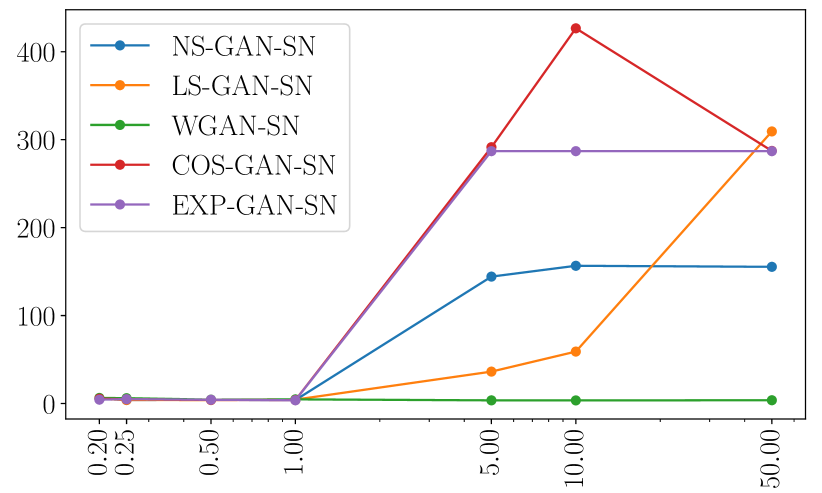
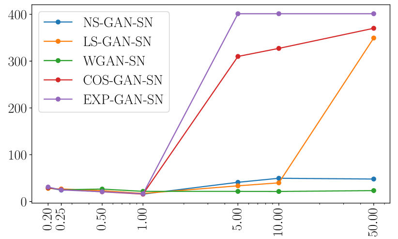
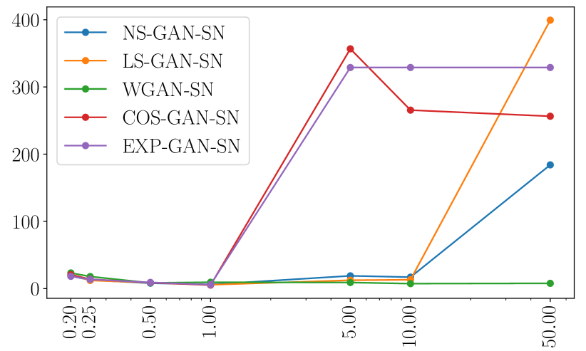
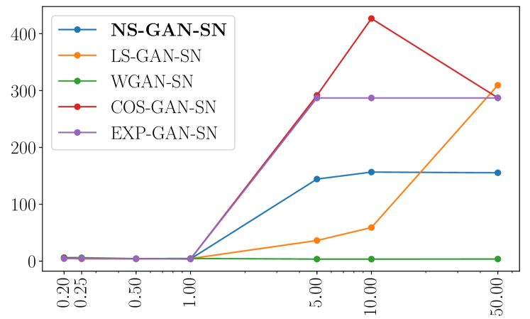
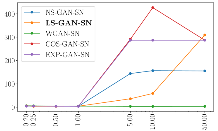
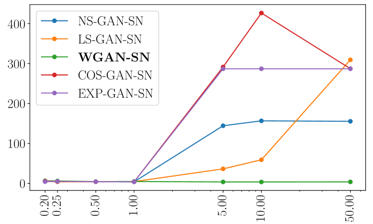
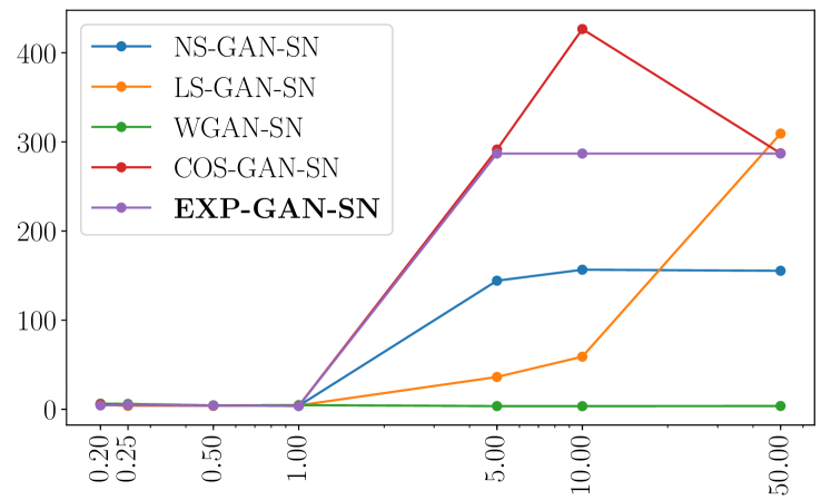
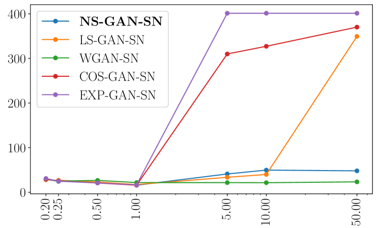
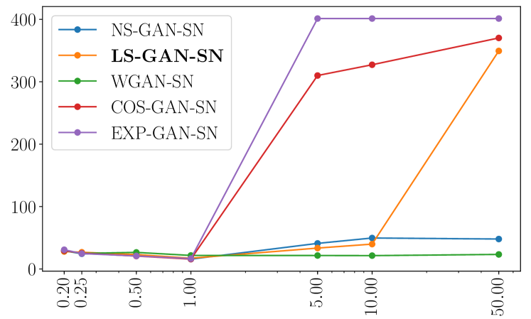
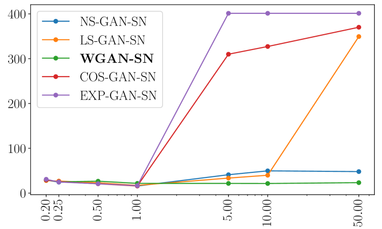
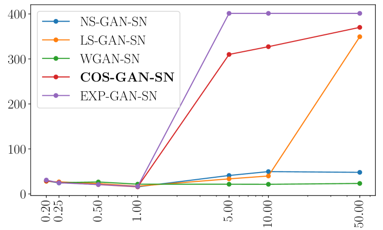
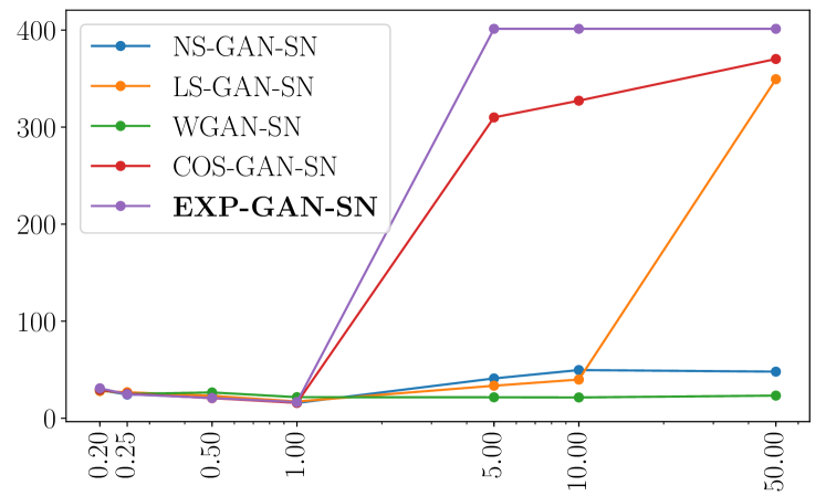
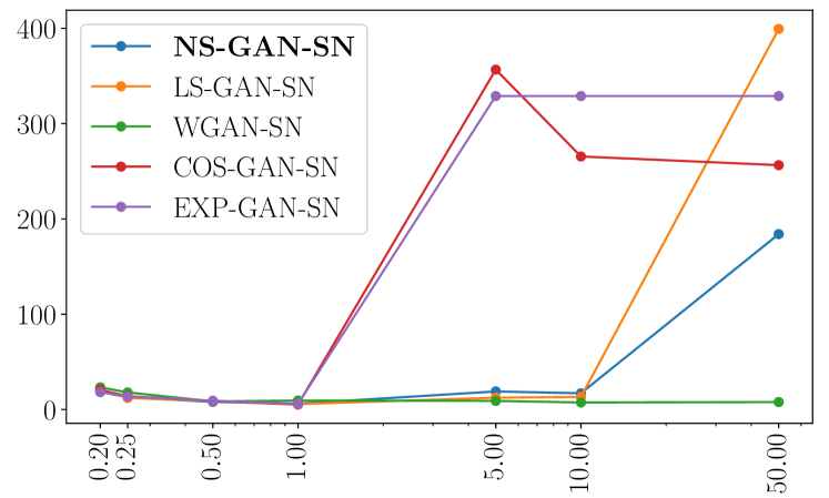
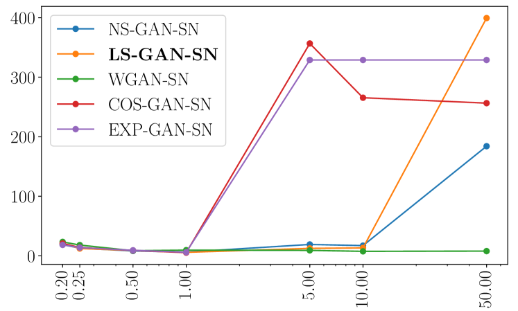
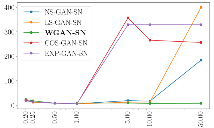
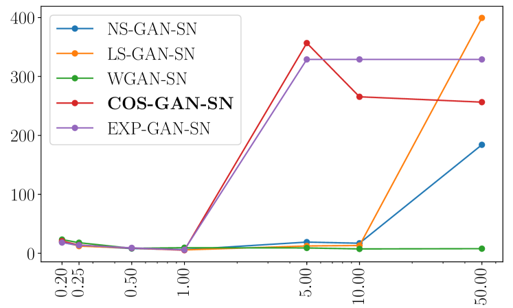
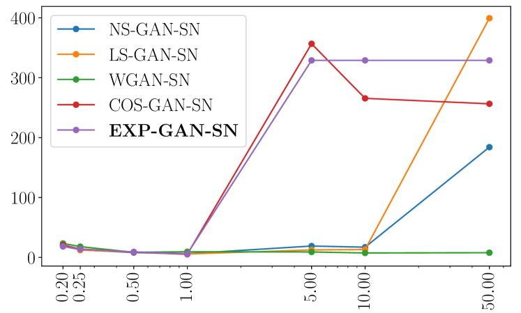
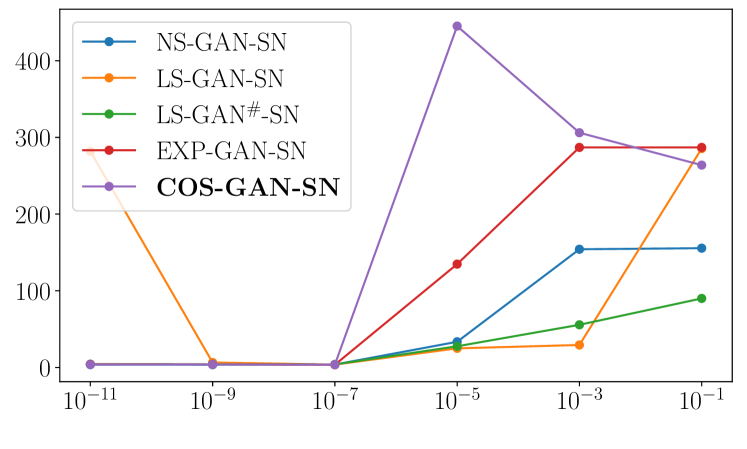
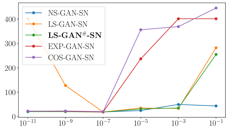
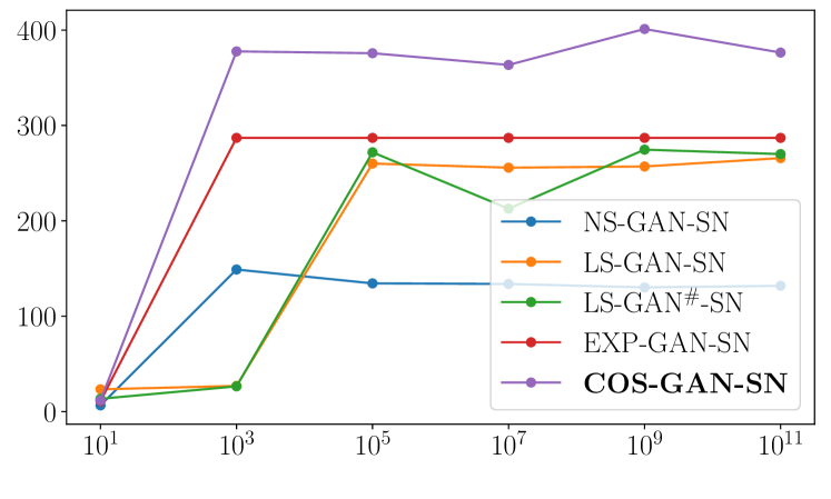
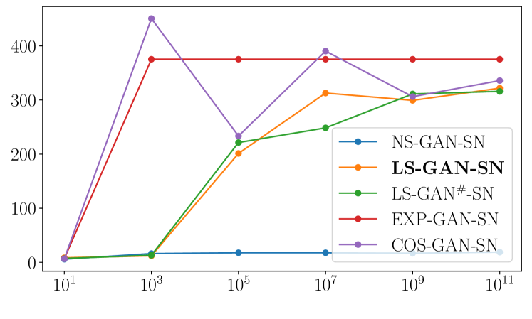
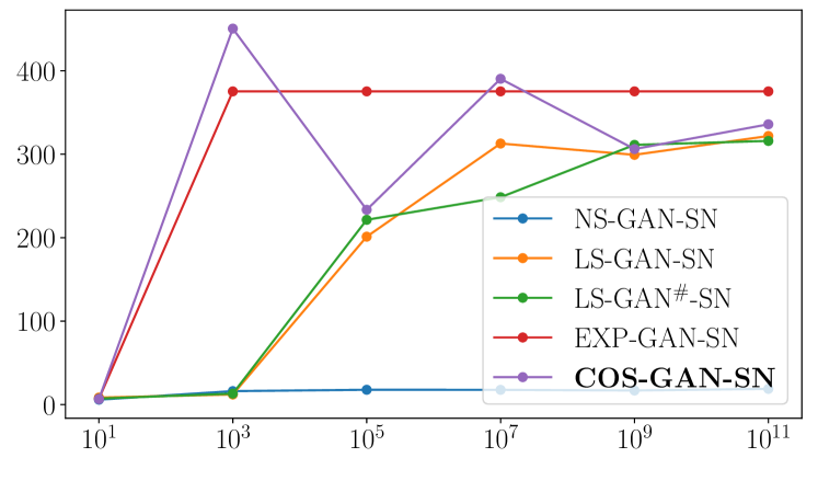
Table 3: FID scores vs. kSNsubscript𝑘𝑆𝑁k_{SN} (typically fixed as 111 [21]) on different datasets. When kSN1.0subscript𝑘𝑆𝑁1.0k_{SN}\leq 1.0, all GANs have similar performance except the WGANs (slightly worse). For the line plots, x𝑥x-axis shows kSNsubscript𝑘𝑆𝑁k_{SN} (in log scale) and y𝑦y-axis shows the FID scores. From left to right, the seven points on each line have kSN=0.2subscript𝑘𝑆𝑁0.2k_{SN}=0.2, 0.250.250.25, 0.50.50.5, 1.01.01.0, 5.05.05.0, 10.010.010.0, 50.050.050.0 respectively. Lower FID scores are better.
Dataset GANs FID Scores
kSNsubscript𝑘𝑆𝑁k_{SN} = 0.2 0.25 0.5 1.0 5.0 10.0 50.0
MNIST NS-GAN-SN 5.41 3.99 4.20 3.90 144.28 156.60 155.41
LS-GAN-SN 5.14 3.96 3.90 4.42 36.26 59.04 309.35
WGAN-SN 6.35 6.06 4.44 4.70 3.58 3.50 3.71
COS-GAN-SN 5.41 4.83 4.05 3.86 291.44 426.62 287.23
EXP-GAN-SN 4.38 4.93 4.25 3.69 286.96 286.96 286.96
CIFAR10 NS-GAN-SN 29.23 24.37 23.29 15.81 41.04 49.67 48.03
LS-GAN-SN 28.04 26.85 23.14 17.30 33.53 39.90 349.35
WGAN-SN 29.20 25.07 26.61 21.75 21.63 21.45 23.36
COS-GAN-SN 29.45 25.31 20.73 15.88 309.96 327.20 370.13
EXP-GAN-SN 30.89 24.74 20.90 16.66 401.24 401.24 401.24
CelebA NS-GAN-SN 18.59 12.71 8.04 6.11 18.95 17.04 184.06
LS-GAN-SN 20.34 12.14 8.85 5.69 12.40 13.14 399.39
WGAN-SN 23.26 17.93 8.48 9.41 9.03 7.37 7.82
COS-GAN-SN 20.59 13.93 8.88 5.20 356.70 265.53 256.44
EXP-GAN-SN 18.23 13.65 9.18 5.88 328.94 328.94 328.94
Refer to caption
(g) MNIST
Refer to caption
(h) CIFAR10
Refer to caption
(i) CelebA
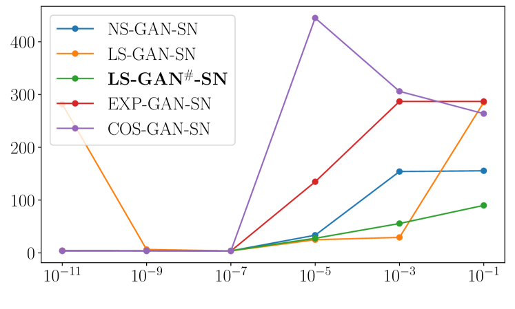
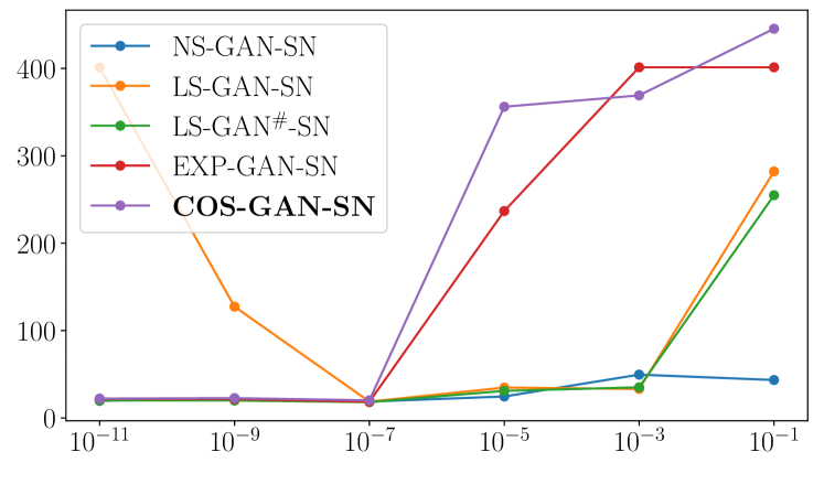
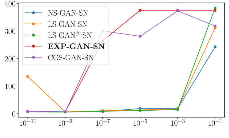
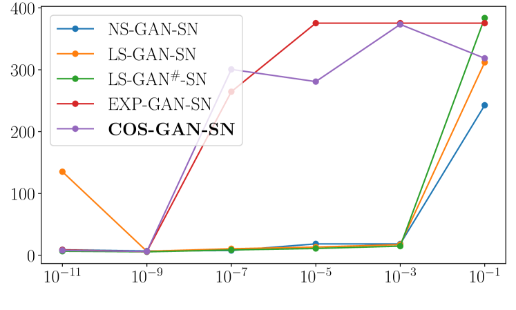
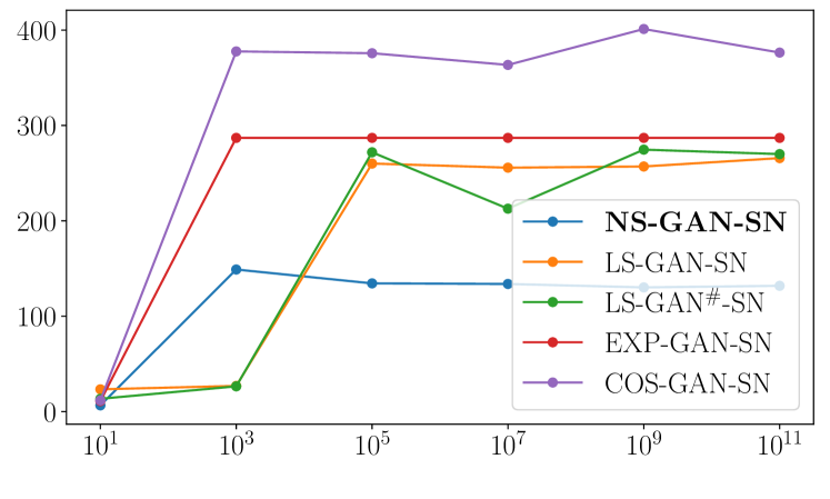
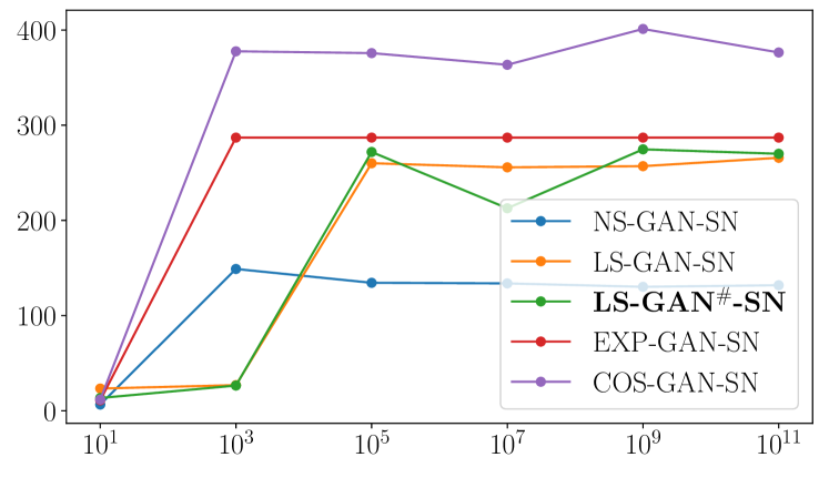
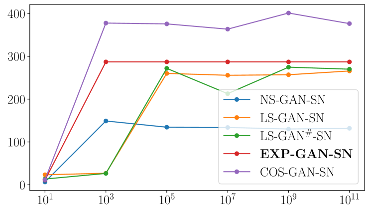
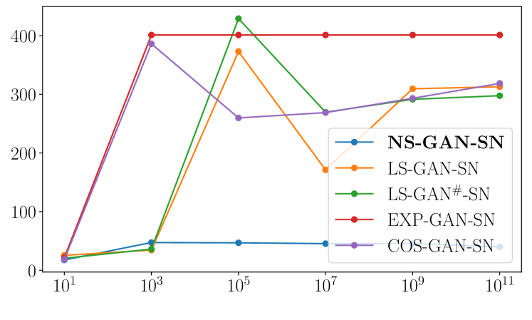
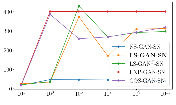
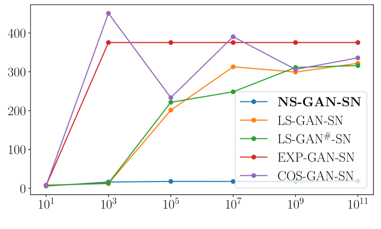
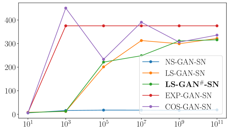
Table 4: FID scores vs. α𝛼\alpha. For the line plots, the x𝑥x-axis shows α𝛼\alpha (in log scale) and the y𝑦y-axis shows the FID scores. Results on other datasets are shown in the supplementary material. Lower FID scores are better.
Dataset GANs FID Scores Line Plot
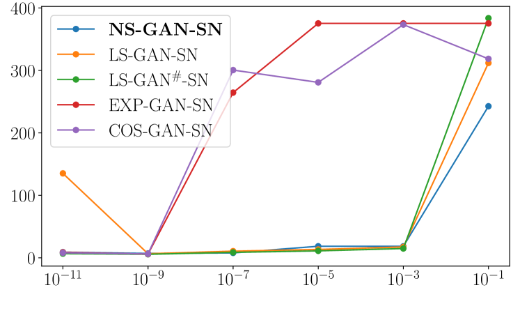
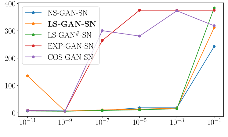
α𝛼\alpha = 1e111superscript𝑒111e^{-11} 1e91superscript𝑒91e^{-9} 1e71superscript𝑒71e^{-7} 1e51superscript𝑒51e^{-5} 1e31superscript𝑒31e^{-3} 1e11superscript𝑒11e^{-1}
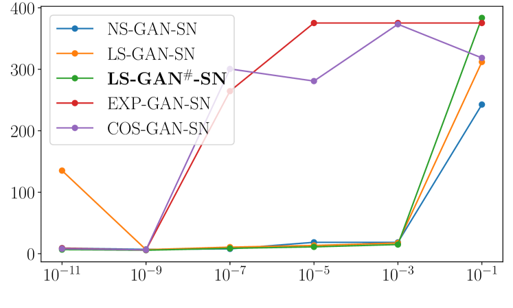
CelebA NS-GAN-SN 9.08 7.05 7.84 18.51 18.41 242.64 [Uncaptioned image]
LS-GAN-SN 135.17 6.57 10.67 13.39 17.42 311.93
LS-GAN#-SN 6.66 5.68 8.72 11.13 14.90 383.61
COS-GAN-SN 8.00 6.31 300.55 280.84 373.31 318.53
EXP-GAN-SN 8.85 6.09 264.49 375.32 375.32 375.32
(a) kSN=50.0subscript𝑘𝑆𝑁50.0k_{SN}=50.0
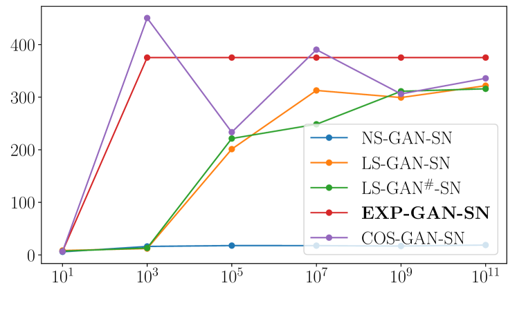
Dataset GANs FID Scores Line Plot
α𝛼\alpha = 1e11superscript𝑒11e^{1} 1e31superscript𝑒31e^{3} 1e51superscript𝑒51e^{5} 1e71superscript𝑒71e^{7} 1e91superscript𝑒91e^{9} 1e111superscript𝑒111e^{11}
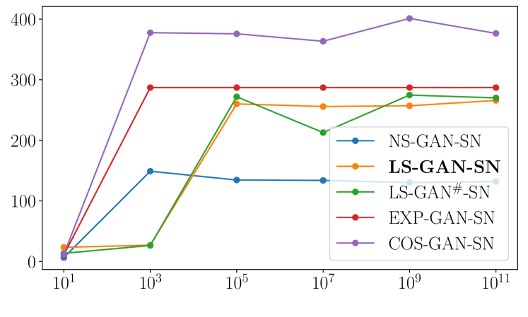
MNIST NS-GAN-SN 6.55 148.97 134.44 133.82 130.21 131.87 [Uncaptioned image]
LS-GAN-SN 23.37 26.96 260.05 255.73 256.96 265.76
LS-GAN#-SN 13.43 26.51 271.85 212.74 274.63 269.96
COS-GAN-SN 11.79 377.62 375.72 363.45 401.12 376.39
EXP-GAN-SN 11.02 286.96 286.96 286.96 286.96 286.96
(b) kSN=1.0subscript𝑘𝑆𝑁1.0k_{SN}=1.0

FID scores vs. Lipschitz Regularization. Table 4(i) shows the FID scores of different GAN loss functions with different kSNsubscript𝑘𝑆𝑁k_{SN}. It can be observed that:

  • When kSN1.0subscript𝑘𝑆𝑁1.0k_{SN}\leq 1.0, all the loss functions (including the non-standard ones) can be used to train GANs stably. However, the FID scores of all loss functions slightly worsen as kSNsubscript𝑘𝑆𝑁k_{SN} decreases. We believe that the reason for such performance degradation comes from the trick used by modern optimizers to avoid divisions by zero. For example in RMSProp [26], the moving average of the squared gradients are kept for each weight. In order to stabilize training, gradients are divided by the square roots of their moving averages in each update of the weights, where a small positive constant ϵitalic-ϵ\epsilon is included in the denominator to avoid dividing by zero. When kSNsubscript𝑘𝑆𝑁k_{SN} is large, the gradients are also large and the effect of ϵitalic-ϵ\epsilon is negligible. While when kSNsubscript𝑘𝑆𝑁k_{SN} is very small, the gradients are also small so that ϵitalic-ϵ\epsilon can significantly slow down the training and worsen the results.

  • When kSN1.0subscript𝑘𝑆𝑁1.0k_{SN}\leq 1.0, the performance of WGAN is slightly worse than almost all the other GANs. Similar to the observation of [12], we ascribe this problem to the shifting domain of WGANs (Figure 4 (c)(f)). The reason for the domain shift is that the Wasserstein distance only depends on the difference between 𝔼[f(x)]𝔼delimited-[]𝑓𝑥\mathbb{E}[f(x)] and 𝔼[f(g(z)]\mathbb{E}[f(g(z)] (Table 1). For example, the Wasserstein distances 𝔼[f(x)]𝔼[f(g(z)]\mathbb{E}[f(x)]-\mathbb{E}[f(g(z)] are the same for i) 𝔼[f(x)]=0.5,𝔼[f(g(z))=0.5\mathbb{E}[f(x)]=0.5,\mathbb{E}[f(g(z))=-0.5 and ii) 𝔼[f(x)]=100.5,𝔼[f(g(z))=99.5\mathbb{E}[f(x)]=100.5,\mathbb{E}[f(g(z))=99.5.

  • When kSN5.0subscript𝑘𝑆𝑁5.0k_{SN}\geq 5.0, the WGAN works normally while the performance of all the other GANs worsen and even break (very high FID scores, e.g. 100absent100\geq 100). The reasons for the stable performance of WGAN are two-fold: i) due to the KR duality, the Wasserstein distance is insensitive to the Lipschitz constant K𝐾K. Let W(r,g)𝑊subscript𝑟subscript𝑔W(\mathbb{P}_{r},\mathbb{P}_{g}) be the Wasserstein distance between the data distribution rsubscript𝑟\mathbb{P}_{r} and the generator distribution gsubscript𝑔\mathbb{P}_{g}. As discussed in [2], applying K𝐾K-Lipschitz regularization to WGAN is equivalent to estimating KW(r,g)𝐾𝑊subscript𝑟subscript𝑔K\cdot W(\mathbb{P}_{r},\mathbb{P}_{g}), which shares the same solution as 111-Lipschitz regularized WGAN. ii) To fight the exploding and vanishing gradient problems, modern neural networks are intentionally designed to be scale-insensitive to the backpropagated gradients (e.g. ReLU [6], RMSProp [26]). This largely eliminates the scaling effect caused by kSNsubscript𝑘𝑆𝑁k_{SN}. This observation also supports our claim that the restriction of the loss function is the dominating factor of the Lipschitz regularization.

  • The best performance is obtained by GANs with strictly convex (e.g. NS-GAN) and properly restricted (e.g. kSN=1subscript𝑘𝑆𝑁1k_{SN}=1) loss functions that address the shifting domain and exploding/vanishing gradient problems at the same time. However, there is no clear preference and even the non-standard ones (e.g., COS-GAN) can be the best. We believe that this is due to the subtle differences of the convexity among loss functions and propose to leave it to the fine-tuning of loss functions using the proposed domain scaling.

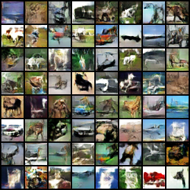
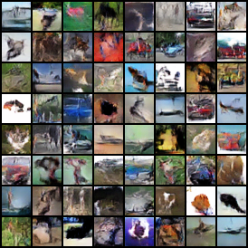
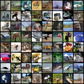
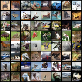
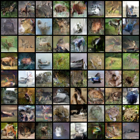
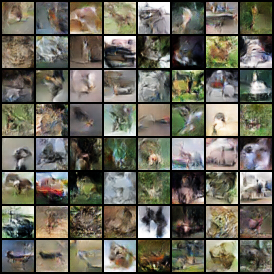
Qualitative results are in the supplementary material.

4.3 Empirical Results on Domain Scaling

In this section, we empirically verify our claim that the restriction of the loss function is the dominating factor of the Lipschitz regularization. To illustrate it, we decouple the restriction of the domain of the loss function from the Lipschitz regularization by the proposed domain scaling method (Section 3.2).

Table 5: FID scores of WGAN-SN and some extremely degenerate loss functions (α=1e25𝛼1superscript𝑒25\alpha=1e^{-25}) on different datasets. We use kSN=50subscript𝑘𝑆𝑁50k_{SN}=50 for all our experiments.
GANs FID Scores
MNIST CIFAR10 CELEBA
WGAN-SN 3.71 23.36 7.82
NS-GAN-SN 3.74 21.92 8.10
LS-GAN#-SN 3.81 21.47 8.51
COS-GAN-SN 3.96 23.65 8.30
EXP-GAN-SN 3.86 21.91 8.22

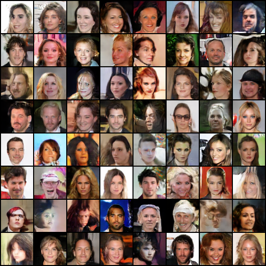
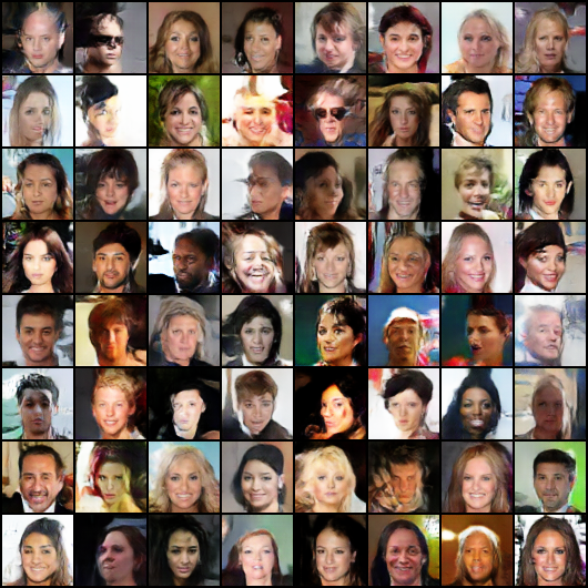
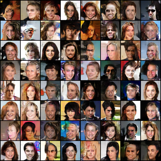
Table 4(b) (a) shows that (i) the FID scores of different loss functions generally improve with decreasing α𝛼\alpha. When α109𝛼superscript109\alpha\leq 10^{-9}, we can successfully train GANs with extremely large Lipschtiz constant (KkSNn=504=6.25×10⁶𝐾superscriptsubscript𝑘𝑆𝑁𝑛superscript5046.25superscript106K\approx k_{SN}^{n}=50^{4}=6.25\times 10^{6}), whose FID scores are comparable to the best ones in Table 4(i). (ii) The FID scores when α1011𝛼superscript1011\alpha\leq 10^{-11} are slightly worse than those when α109𝛼superscript109\alpha\leq 10^{-9}. The reason for this phenomenon is that restricting the domain of the loss function converges towards the performance of WGAN, which is slightly worse than the others due to its shifting domain. To further illustrate this point, we scale the domain by α=1e25𝛼1superscript𝑒25\alpha=1e^{-25} and show the FID scores of WGAN-SN and those of different loss functions in Table 5. It can be observed that all loss functions have similar performance. Since domain scaling does not restrict the neural network gradients, it does not suffer from the above-mentioned numerical problem of division by zero (kSN1.0subscript𝑘𝑆𝑁1.0k_{SN}\leq 1.0, Table 4(i)). Thus, it is a better alternative to tuning kSNsubscript𝑘𝑆𝑁k_{SN}.

Table 4(b) (b) shows that the FID scores of different loss functions generally worsen with less restricted domains. Note that when α105𝛼superscript105\alpha\geq 10^{5}, the common practice of 111-Lipschitz regularization fails to stabilize the GAN training. Note that the LS-GAN-SN has some abnormal behavior (e.g. α=1e11𝛼1superscript𝑒11\alpha=1e^{-11} in Table 4(b) (a) and α=1e1𝛼1superscript𝑒1\alpha=1e^{1} in Table 4(b) (b)) due to the conflict between its 0.50.50.5-centered domain and our zero-centered domain scaling method (Eq.8). This can be easily fixed by using the zero-centered LS-GAN#-SN (see Table 1).
Refer to caption
(a) NS-GAN-SN
Refer to caption
(b) LS-GAN-SN
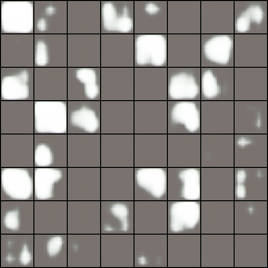
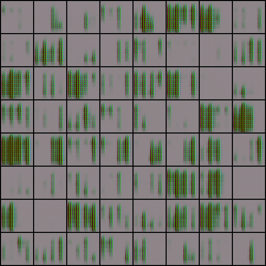
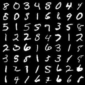
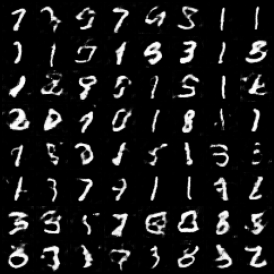
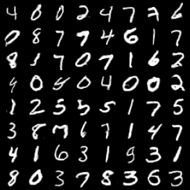
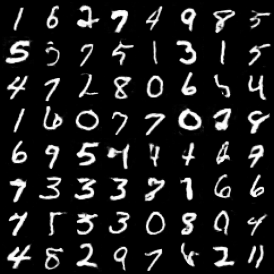
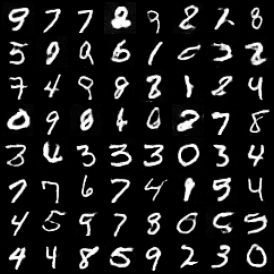
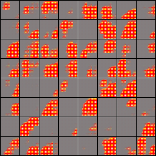
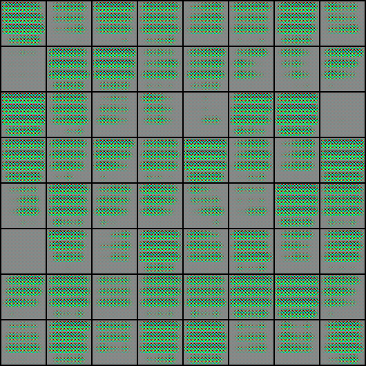
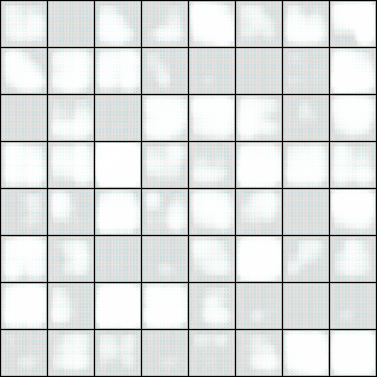
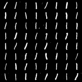
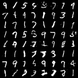
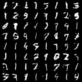
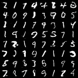
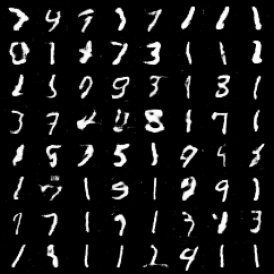
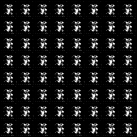
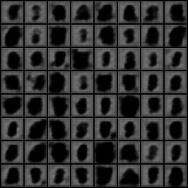
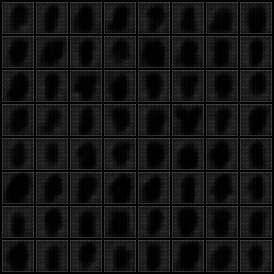
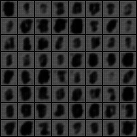
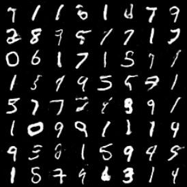
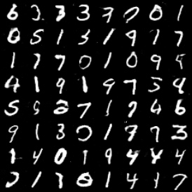
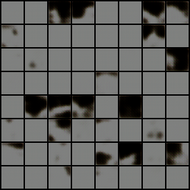
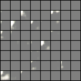
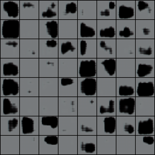
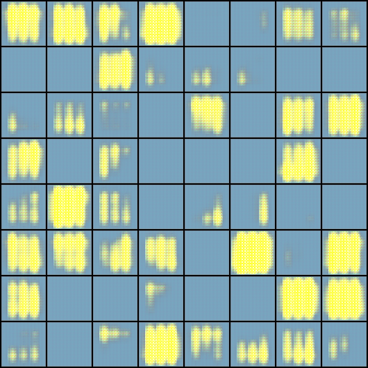
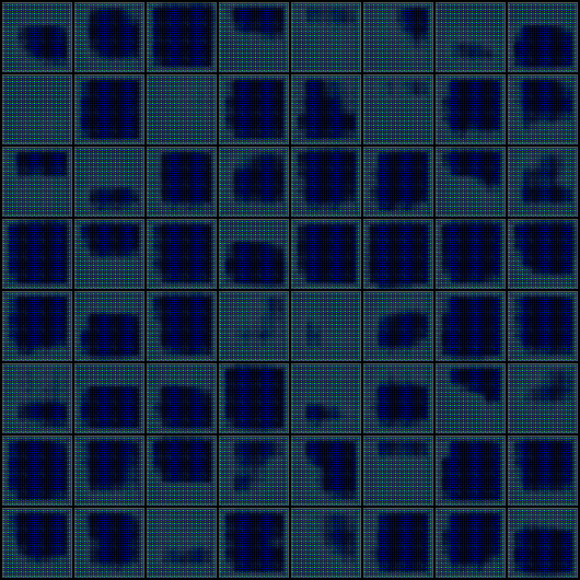
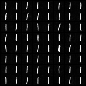
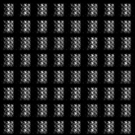
Figure 5: (a) Mode collapse and (b) crashed training on MNIST, kSN=50.0subscript𝑘𝑆𝑁50.0k_{SN}=50.0, α=1e1𝛼1superscript𝑒1\alpha=1e^{-1}.

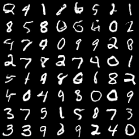
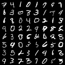
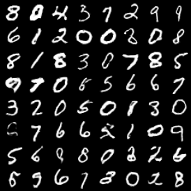
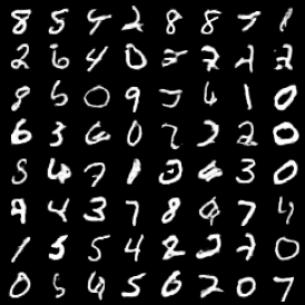
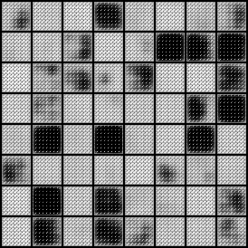
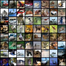
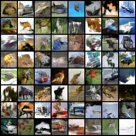
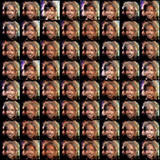
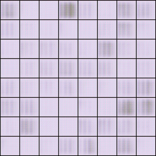
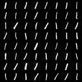
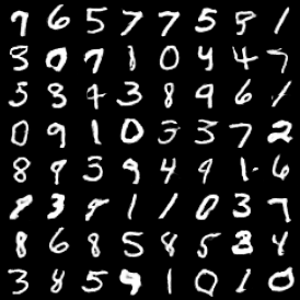
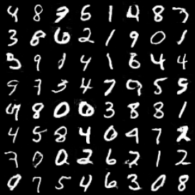
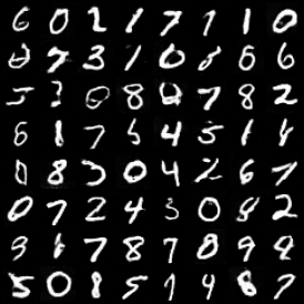
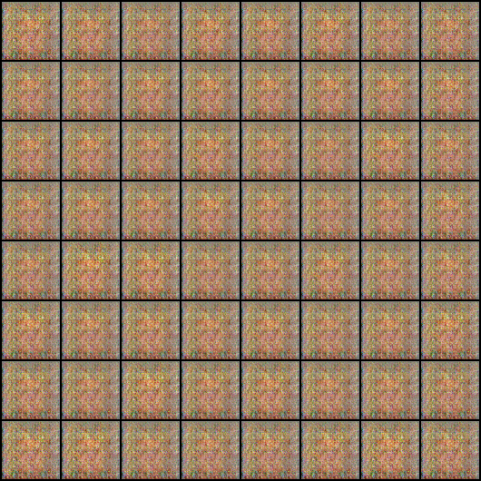
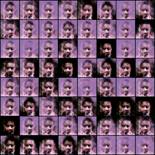
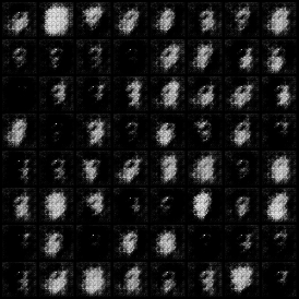
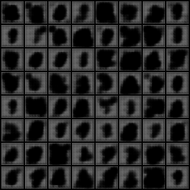
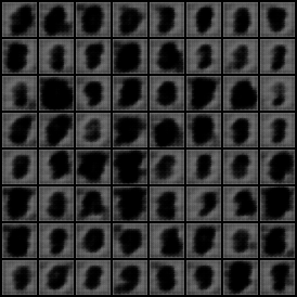
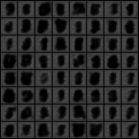
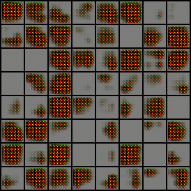
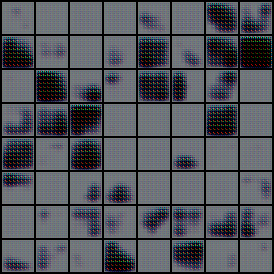
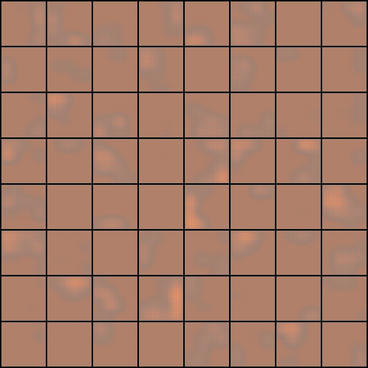
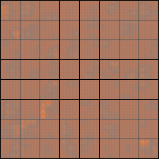
Bias over Input Samples. When weak Lipschitz regularization (large Lipschitz constant K𝐾K) is applied, we observed mode collapse for NS-GAN and crashed training for LS-GAN, EXP-GAN and COS-GAN (Figure 5, more results in supplementary material). We conjecture that this phenomenon is rooted in the inherent bias of neural networks over input samples: neural networks may “prefer” some input (class of) samples over the others by outputting higher/lower values, even though all of them are real samples from the training dataset. When the above-mentioned loss functions are used, such different outputs result in different backpropagated gradients L=D(f(x))/f(x)𝐿𝐷𝑓𝑥𝑓𝑥\nabla L=\partial D(f(x))/\partial f(x). The use of weak Lipschitz regularization further enhances the degree of unbalance among backpropagated gradients and causes mode collapse or crashed training. Note that mode collapse happens when L𝐿\nabla L is bounded (e.g. NS-GAN) and crashed training happens when L𝐿\nabla L is unbounded (e.g. LS-GAN, EXP-GAN) or “random” (e.g. COS-GAN). However, when strong Lipschitz regularization is applied, all loss functions degenerate to almost linear ones and balance the backpropagated gradients, thereby improve the training.

5 Conclusion

In this paper, we studied the coupling of Lipschitz regularization and the loss function. Our key insight is that instead of keeping the neural network gradients small, the dominating factor of Lipschitz regularization is its restriction on the domain and interval of attainable gradient values of the loss function. Such restrictions stabilize GAN training by avoiding the bias of the loss function over input samples, which is a new step in understanding the exact reason for Lipschitz regularization’s effectiveness. Furthermore, our finding suggests that although different loss functions can be used to train GANs successfully, they actually work in the same way because all of them degenerate to near-linear ones within the chosen small domains.

Acknowledgement This work was supported in part by the KAUST Office of Sponsored Research (OSR) under Award No. OSR-CRG2018-3730.

References

  • [1] Arjovsky, M., Bottou, L.: Towards principled methods for training generative adversarial networks. In: International Conference on Learning Representations (2017)
  • [2] Arjovsky, M., Chintala, S., Bottou, L.: Wasserstein generative adversarial networks. In: Precup, D., Teh, Y.W. (eds.) Proceedings of the 34th International Conference on Machine Learning. Proceedings of Machine Learning Research, vol. 70, pp. 214–223. PMLR, International Convention Centre, Sydney, Australia (06–11 Aug 2017), http://proceedings.mlr.press/v70/arjovsky17a.html
  • [3] Barratt, S., Sharma, R.: A note on the inception score. arXiv preprint arXiv:1801.01973 (2018)
  • [4] Fedus*, W., Rosca*, M., Lakshminarayanan, B., Dai, A.M., Mohamed, S., Goodfellow, I.: Many paths to equilibrium: GANs do not need to decrease a divergence at every step. In: International Conference on Learning Representations (2018), https://openreview.net/forum?id=ByQpn1ZA-
  • [5] Frühstück, A., Alhashim, I., Wonka, P.: Tilegan: Synthesis of large-scale non-homogeneous textures. ACM Trans. Graph. 38(4) (Jul 2019). https://doi.org/10.1145/3306346.3322993
  • [6] Glorot, X., Bordes, A., Bengio, Y.: Deep sparse rectifier neural networks. In: Gordon, G., Dunson, D., Dudík, M. (eds.) Proceedings of the Fourteenth International Conference on Artificial Intelligence and Statistics. Proceedings of Machine Learning Research, vol. 15, pp. 315–323. PMLR, Fort Lauderdale, FL, USA (11–13 Apr 2011), http://proceedings.mlr.press/v15/glorot11a.html
  • [7] Goodfellow, I., Pouget-Abadie, J., Mirza, M., Xu, B., Warde-Farley, D., Ozair, S., Courville, A., Bengio, Y.: Generative adversarial nets. In: Ghahramani, Z., Welling, M., Cortes, C., Lawrence, N.D., Weinberger, K.Q. (eds.) Advances in Neural Information Processing Systems 27, pp. 2672–2680. Curran Associates, Inc. (2014), http://papers.nips.cc/paper/5423-generative-adversarial-nets.pdf
  • [8] Gulrajani, I., Ahmed, F., Arjovsky, M., Dumoulin, V., Courville, A.C.: Improved training of wasserstein gans. In: Guyon, I., Luxburg, U.V., Bengio, S., Wallach, H., Fergus, R., Vishwanathan, S., Garnett, R. (eds.) Advances in Neural Information Processing Systems 30, pp. 5767–5777. Curran Associates, Inc. (2017), http://papers.nips.cc/paper/7159-improved-training-of-wasserstein-gans.pdf
  • [9] Gulrajani, I., Raffel, C., Metz, L.: Towards GAN benchmarks which require generalization. In: International Conference on Learning Representations (2019), https://openreview.net/forum?id=HkxKH2AcFm
  • [10] He, K., Zhang, X., Ren, S., Sun, J.: Deep residual learning for image recognition. In: Proceedings of the IEEE Conference on Computer Vision and Pattern Recognition (CVPR) (June 2016)
  • [11] Heusel, M., Ramsauer, H., Unterthiner, T., Nessler, B., Hochreiter, S.: Gans trained by a two time-scale update rule converge to a local nash equilibrium. In: Guyon, I., Luxburg, U.V., Bengio, S., Wallach, H., Fergus, R., Vishwanathan, S., Garnett, R. (eds.) Advances in Neural Information Processing Systems 30, pp. 6626–6637. Curran Associates, Inc. (2017), http://papers.nips.cc/paper/7240-gans-trained-by-a-two-time-scale-update-rule-converge-to-a-local-nash-equilibrium.pdf
  • [12] Karras, T., Aila, T., Laine, S., Lehtinen, J.: Progressive growing of GANs for improved quality, stability, and variation. In: International Conference on Learning Representations (2018), https://openreview.net/forum?id=Hk99zCeAb
  • [13] Kelly, T., Guerrero, P., Steed, A., Wonka, P., Mitra, N.J.: Frankengan: Guided detail synthesis for building mass models using style-synchonized gans. ACM Trans. Graph. 37(6) (Dec 2018). https://doi.org/10.1145/3272127.3275065, https://doi.org/10.1145/3272127.3275065
  • [14] Kurach, K., Lucic, M., Zhai, X., Michalski, M., Gelly, S.: The GAN landscape: Losses, architectures, regularization, and normalization (2019), https://openreview.net/forum?id=rkGG6s0qKQ
  • [15] Liu, Z., Luo, P., Wang, X., Tang, X.: Deep learning face attributes in the wild. In: Proceedings of the IEEE International Conference on Computer Vision (ICCV) (December 2015)
  • [16] Lucic, M., Kurach, K., Michalski, M., Gelly, S., Bousquet, O.: Are gans created equal? a large-scale study. In: Bengio, S., Wallach, H., Larochelle, H., Grauman, K., Cesa-Bianchi, N., Garnett, R. (eds.) Advances in Neural Information Processing Systems 31, pp. 700–709. Curran Associates, Inc. (2018), http://papers.nips.cc/paper/7350-are-gans-created-equal-a-large-scale-study.pdf
  • [17] Ma, L., Jia, X., Sun, Q., Schiele, B., Tuytelaars, T., Van Gool, L.: Pose guided person image generation. In: Guyon, I., Luxburg, U.V., Bengio, S., Wallach, H., Fergus, R., Vishwanathan, S., Garnett, R. (eds.) Advances in Neural Information Processing Systems 30, pp. 406–416. Curran Associates, Inc. (2017), http://papers.nips.cc/paper/6644-pose-guided-person-image-generation.pdf
  • [18] Mao, X., Li, Q., Xie, H., Lau, R.Y.K., Wang, Z., Smolley, S.P.: On the effectiveness of least squares generative adversarial networks. IEEE Transactions on Pattern Analysis and Machine Intelligence 41(12), 2947–2960 (2019)
  • [19] Mao, X., Li, Q., Xie, H., Lau, R.Y., Wang, Z., Paul Smolley, S.: Least squares generative adversarial networks. In: Proceedings of the IEEE International Conference on Computer Vision (ICCV) (Oct 2017)
  • [20] Mescheder, L., Geiger, A., Nowozin, S.: Which training methods for GANs do actually converge? In: Dy, J., Krause, A. (eds.) Proceedings of the 35th International Conference on Machine Learning. Proceedings of Machine Learning Research, vol. 80, pp. 3481–3490. PMLR, Stockholmsmässan, Stockholm Sweden (10–15 Jul 2018), http://proceedings.mlr.press/v80/mescheder18a.html
  • [21] Miyato, T., Kataoka, T., Koyama, M., Yoshida, Y.: Spectral normalization for generative adversarial networks. In: International Conference on Learning Representations (2018), https://openreview.net/forum?id=B1QRgziT-
  • [22] Nowozin, S., Cseke, B., Tomioka, R.: f-gan: Training generative neural samplers using variational divergence minimization. In: Lee, D.D., Sugiyama, M., Luxburg, U.V., Guyon, I., Garnett, R. (eds.) Advances in Neural Information Processing Systems 29, pp. 271–279. Curran Associates, Inc. (2016), http://papers.nips.cc/paper/6066-f-gan-training-generative-neural-samplers-using-variational-divergence-minimization.pdf
  • [23] Park, T., Liu, M.Y., Wang, T.C., Zhu, J.Y.: Semantic image synthesis with spatially-adaptive normalization. In: Proceedings of the IEEE/CVF Conference on Computer Vision and Pattern Recognition (CVPR) (June 2019)
  • [24] Radford, A., Metz, L., Chintala, S.: Unsupervised representation learning with deep convolutional generative adversarial networks. arXiv preprint arXiv:1511.06434 (2015)
  • [25] Sanyal, A., Torr, P.H., Dokania, P.K.: Stable rank normalization for improved generalization in neural networks and gans. In: International Conference on Learning Representations (2020), https://openreview.net/forum?id=H1enKkrFDB
  • [26] Tieleman, T., Hinton, G.: Lecture 6.5-rmsprop: Divide the gradient by a running average of its recent magnitude. COURSERA: Neural networks for machine learning 4(2), 26–31 (2012)
  • [27] Wang, T.C., Liu, M.Y., Zhu, J.Y., Tao, A., Kautz, J., Catanzaro, B.: High-resolution image synthesis and semantic manipulation with conditional gans. In: Proceedings of the IEEE Conference on Computer Vision and Pattern Recognition (CVPR) (June 2018)
  • [28] Wu, J., Zhang, C., Xue, T., Freeman, B., Tenenbaum, J.: Learning a probabilistic latent space of object shapes via 3d generative-adversarial modeling. In: Lee, D.D., Sugiyama, M., Luxburg, U.V., Guyon, I., Garnett, R. (eds.) Advances in Neural Information Processing Systems 29, pp. 82–90. Curran Associates, Inc. (2016), http://papers.nips.cc/paper/6096-learning-a-probabilistic-latent-space-of-object-shapes-via-3d-generative-adversarial-modeling.pdf
  • [29] Zhu, J.Y., Park, T., Isola, P., Efros, A.A.: Unpaired image-to-image translation using cycle-consistent adversarial networks. In: Proceedings of the IEEE International Conference on Computer Vision (ICCV) (Oct 2017)

How does Lipschitz Regularization Influence GAN Training?
- Supplementary Material -

Yipeng Qin Niloy Mitra Peter Wonka

6 Detailed Network Architectures

The detailed network architectures of the generators and the discriminators are shown in Table 6.

7 Additional Quantitative Results

Table 7(b) shows the FID scores against α𝛼\alpha on all the three datasets (MNIST, CIFAR10 and CelebA), which is complementary to Table 4 in the main paper. The discussion in the main paper also applies to the additional results in Table 7(b).

We further verified the influence of domain scaling on the CIFAR10 dataset with different Lipschitz regularizers, i.e. Spectral Normalization (SN) [21] and Stable Rank Normalization (SRN)+SN [25], using additional metrics, i.e. Inception Scores (IS) [3] and Neural Divergence (ND) [9]. Specifically, we set kSN=1subscript𝑘𝑆𝑁1k_{SN}=1 for SN, c=0.7𝑐0.7c=0.7 for SRN and reported both IS and ND scores with different α𝛼\alpha. As Table 8(b) and Table 9(b) show,

  • When α𝛼\alpha is small, all loss functions degenerate to linear ones like WGAN and have similar IS and ND scores.

  • When α𝛼\alpha is large, different loss functions behave differently and have different IS, ND scores (mostly worse).

Thus, our conclusions still hold in these settings.

8 Additional Qualitative Results

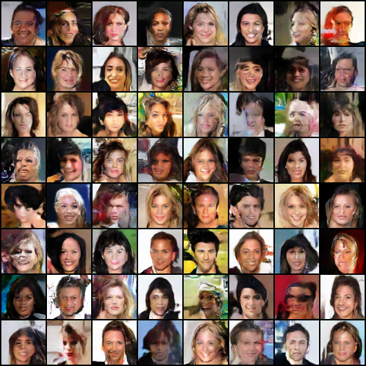
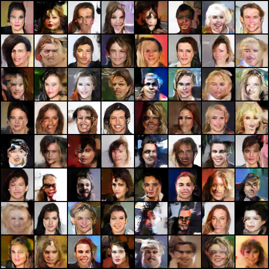
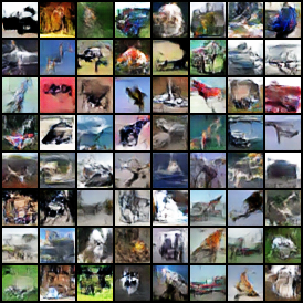
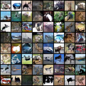
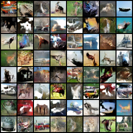
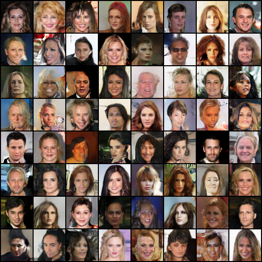
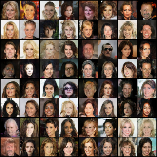
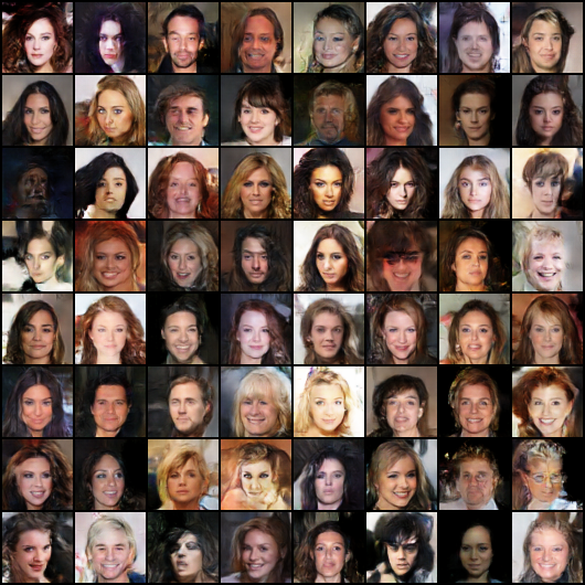
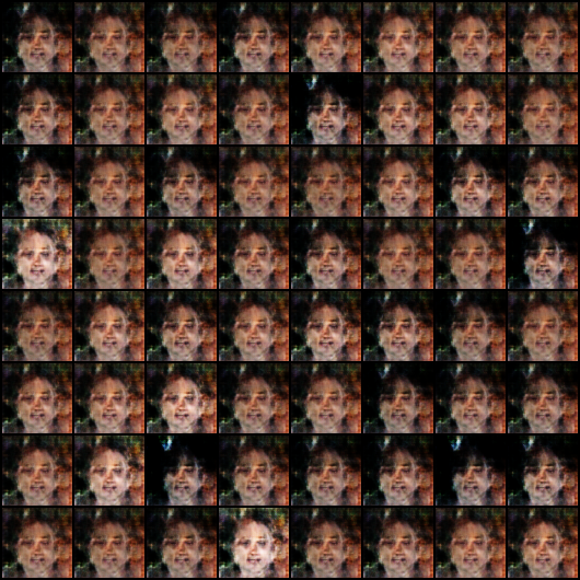
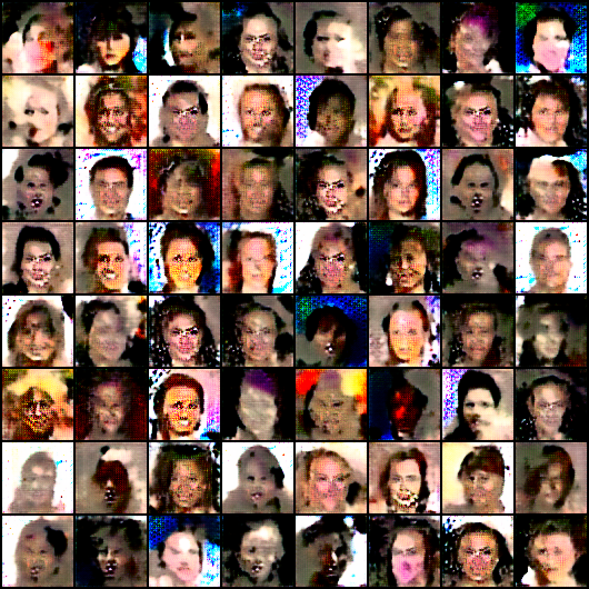
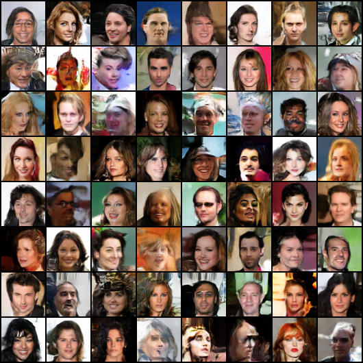
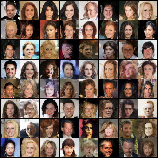
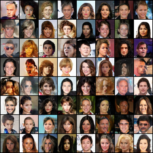
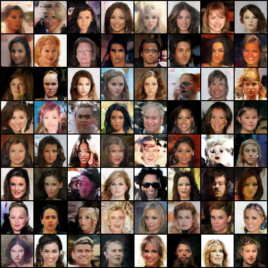
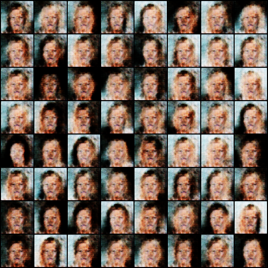
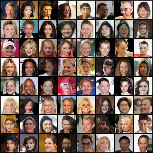
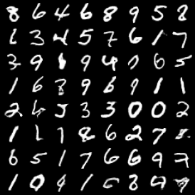
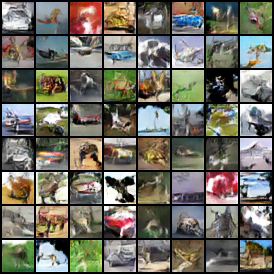
In this section, we show the qualitative results (sample images) corresponding to the quantitative experiments in the main paper. The FID scores and line plots are shown together with the samples.

8.1 Samples of FID scores v.s. kSNsubscript𝑘𝑆𝑁k_{SN} Experiment

This subsection corresponds to the FID scores v.s. kSNsubscript𝑘𝑆𝑁k_{SN} experiment (Table 3 in the main paper).

With varying kSNsubscript𝑘𝑆𝑁k_{SN} on the MNIST dataset,

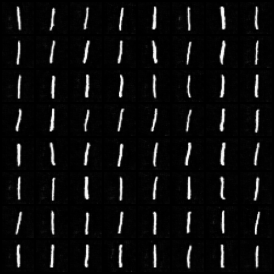
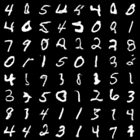
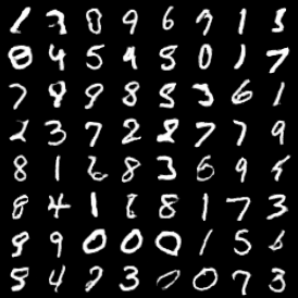
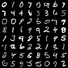
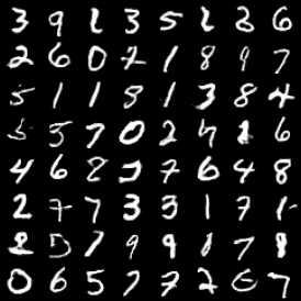
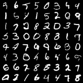
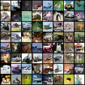
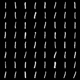
  • Figure 6 shows sample images of the NS-GAN-SN;

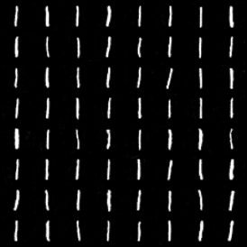
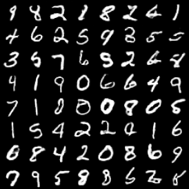
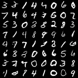
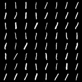
  • Figure 7 shows sample images of the LS-GAN-SN;

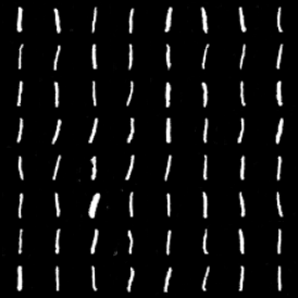
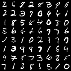
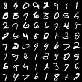
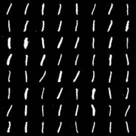
  • Figure 8 shows sample images of the WGAN-SN;

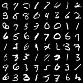
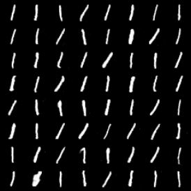
  • Figure 9 shows sample images of the COS-GAN-SN;

  • Figure 10 shows sample images of the EXP-GAN-SN.

With varying kSNsubscript𝑘𝑆𝑁k_{SN} on the CIFAR10 dataset,

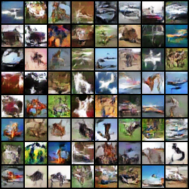
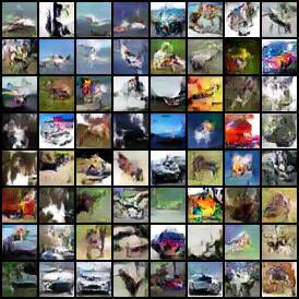
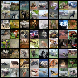
  • Figure 11 shows sample images of the NS-GAN-SN;

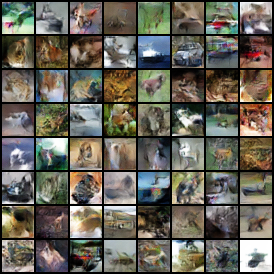
  • Figure 12 shows sample images of the LS-GAN-SN;

  • Figure 13 shows sample images of the WGAN-SN;

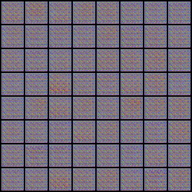
  • Figure 14 shows sample images of the COS-GAN-SN;

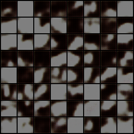
  • Figure 15 shows sample images of the EXP-GAN-SN.

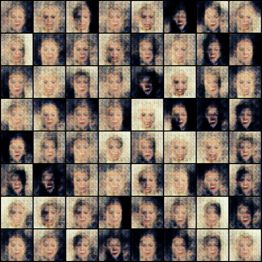
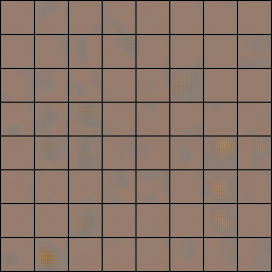
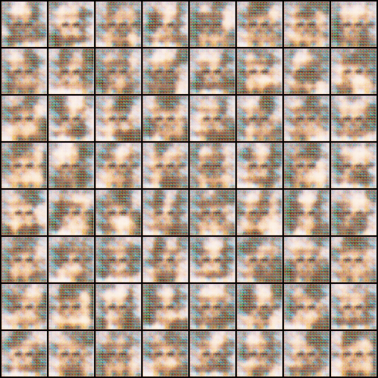
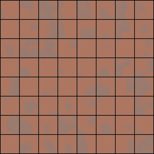
With varying kSNsubscript𝑘𝑆𝑁k_{SN} on the CelebA dataset,

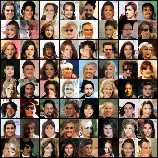
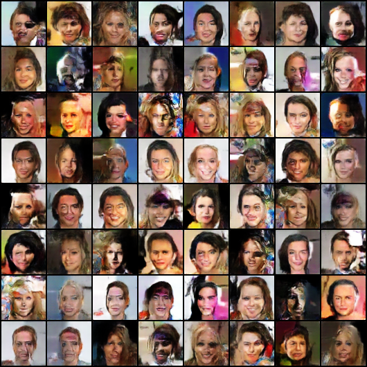
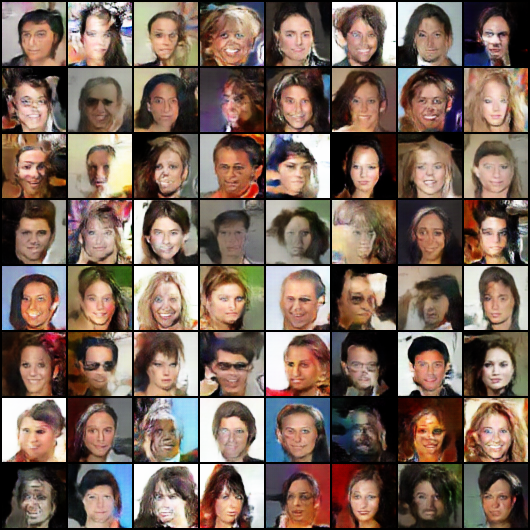
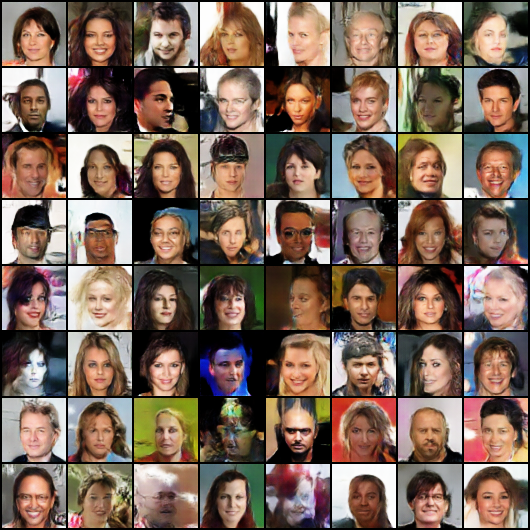
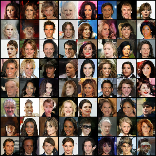
  • Figure 16 shows sample images of the NS-GAN-SN;

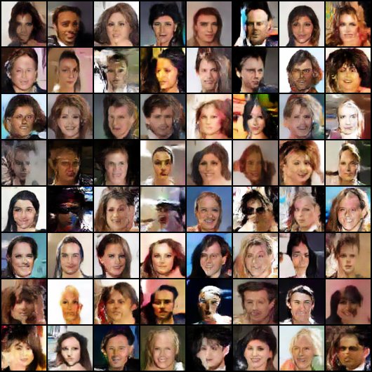
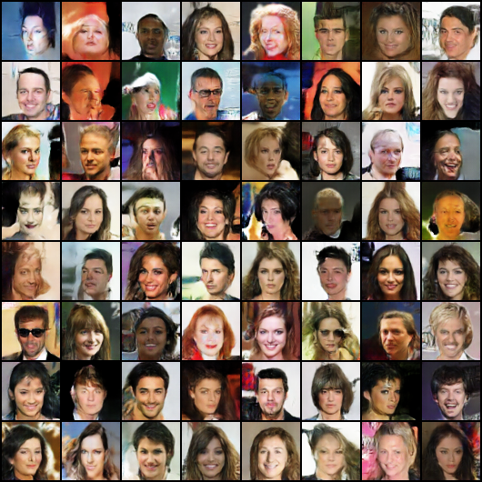
  • Figure 17 shows sample images of the LS-GAN-SN;

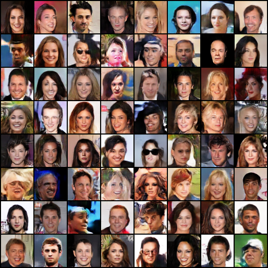
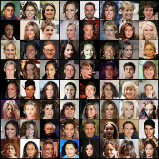
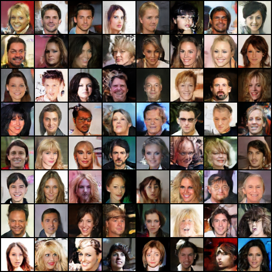
  • Figure 18 shows sample images of the WGAN-SN;

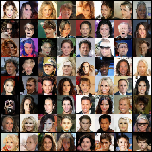
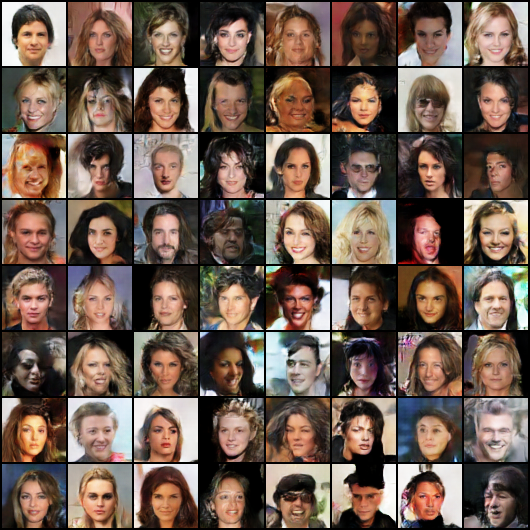
  • Figure 19 shows sample images of the COS-GAN-SN;

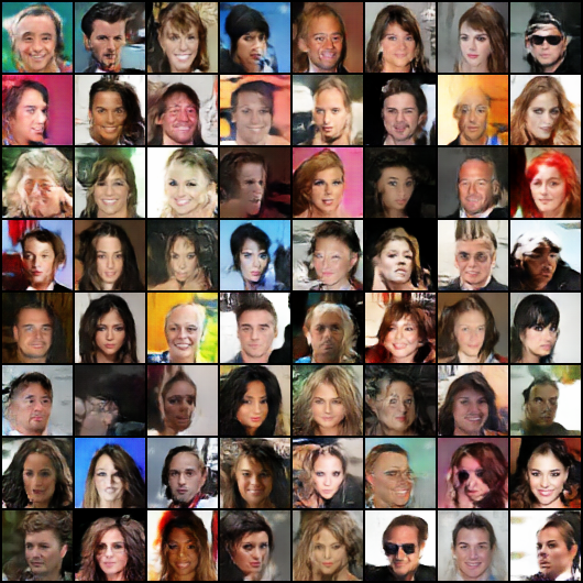
  • Figure 20 shows sample images of the EXP-GAN-SN.

8.2 Samples of the FID scores v.s. α𝛼\alpha Experiment

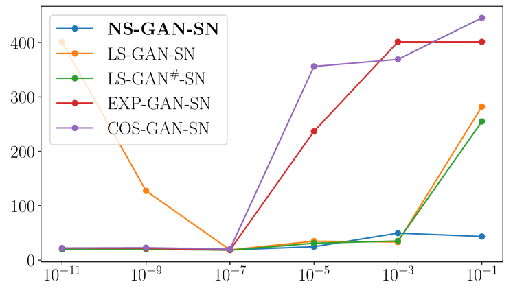
This subsection corresponds to the FID scores v.s. α𝛼\alpha experiment (Table 7(b)). The results show that instead of the restriction of the neural network gradients, the restriction of the loss function is the dominating factor of Lipschitz regularization.

Results for Table 7(b) (a)

With varying α𝛼\alpha, kSN=50.0subscript𝑘𝑆𝑁50.0k_{SN}=50.0 and on MNIST dataset,

  • Figure 21 shows sample images of the NS-GAN-SN;

  • Figure 22 shows sample images of the LS-GAN-SN;

  • Figure 23 shows sample images of the LS-GAN#-SN;

  • Figure 24 shows sample images of the EXP-GAN-SN;

  • Figure 25 shows sample images of the COS-GAN-SN.

With varying α𝛼\alpha, kSN=50.0subscript𝑘𝑆𝑁50.0k_{SN}=50.0 and on CIFAR10 dataset,

  • Figure 26 shows sample images of the NS-GAN-SN;

  • Figure 27 shows sample images of the LS-GAN-SN;

  • Figure 28 shows sample images of the LS-GAN#-SN;

  • Figure 29 shows sample images of the EXP-GAN-SN;

  • Figure 30 shows sample images of the COS-GAN-SN.

With varying α𝛼\alpha, kSN=50.0subscript𝑘𝑆𝑁50.0k_{SN}=50.0 and on CelebA dataset,

  • Figure 31 shows sample images of the NS-GAN-SN;

  • Figure 32 shows sample images of the LS-GAN-SN;

  • Figure 33 shows sample images of the LS-GAN#-SN;

  • Figure 34 shows sample images of the EXP-GAN-SN;

  • Figure 35 shows sample images of the COS-GAN-SN.

Results for Table 7(b) (b)

With varying α𝛼\alpha, kSN=1.0subscript𝑘𝑆𝑁1.0k_{SN}=1.0 and on MNIST dataset,

  • Figure 36 shows sample images of the NS-GAN-SN;

  • Figure 37 shows sample images of the LS-GAN-SN;

  • Figure 38 shows sample images of the LS-GAN#-SN;

  • Figure 39 shows sample images of the EXP-GAN-SN;

  • Figure 40 shows sample images of the COS-GAN-SN.

With varying α𝛼\alpha, kSN=1.0subscript𝑘𝑆𝑁1.0k_{SN}=1.0 and on CIFAR10 dataset,

  • Figure 41 shows sample images of the NS-GAN-SN;

  • Figure 42 shows sample images of the LS-GAN-SN;

  • Figure 43 shows sample images of the LS-GAN#-SN;

  • Figure 44 shows sample images of the EXP-GAN-SN;

  • Figure 45 shows sample images of the COS-GAN-SN.

With varying α𝛼\alpha, kSN=1.0subscript𝑘𝑆𝑁1.0k_{SN}=1.0 and on CelebA dataset,

  • Figure 46 shows sample images of the NS-GAN-SN;

  • Figure 47 shows sample images of the LS-GAN-SN;

  • Figure 48 shows sample images of the LS-GAN#-SN;

  • Figure 49 shows sample images of the EXP-GAN-SN;

  • Figure 50 shows sample images of the COS-GAN-SN.

8.3 Samples of the Degenerate Loss Function

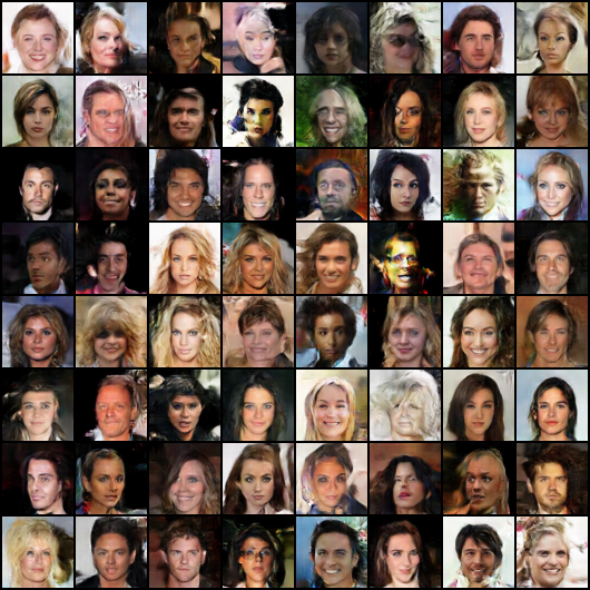
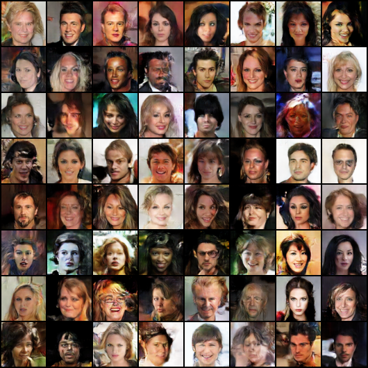
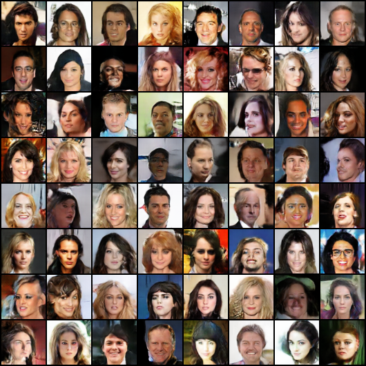
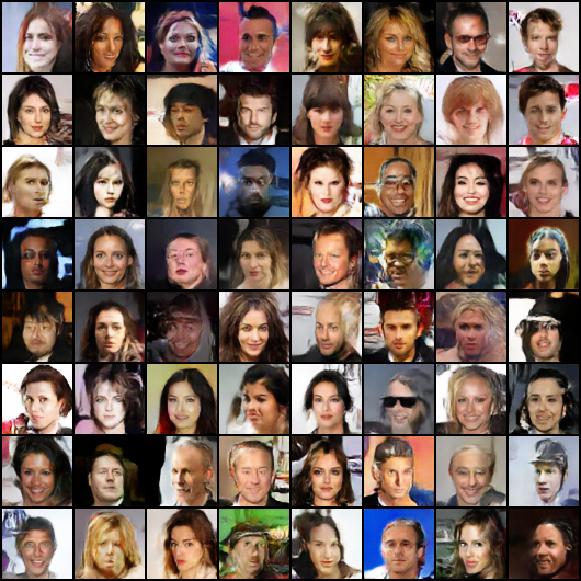
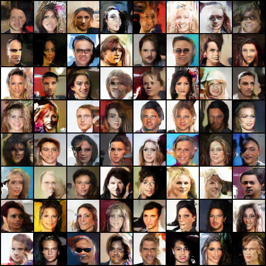
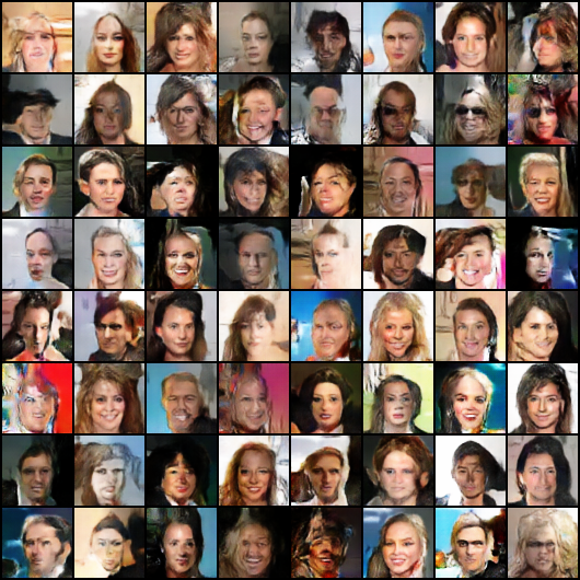
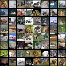
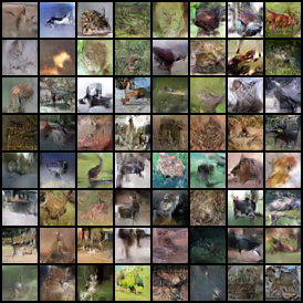
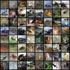
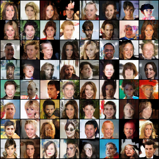
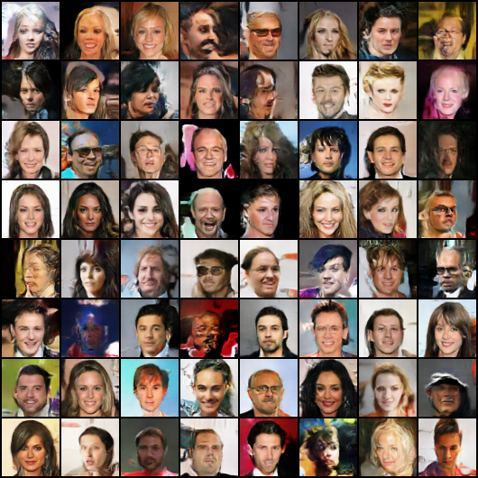
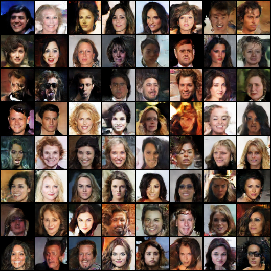
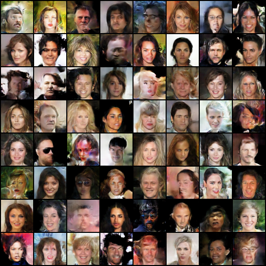
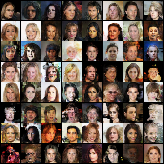
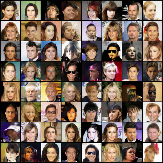
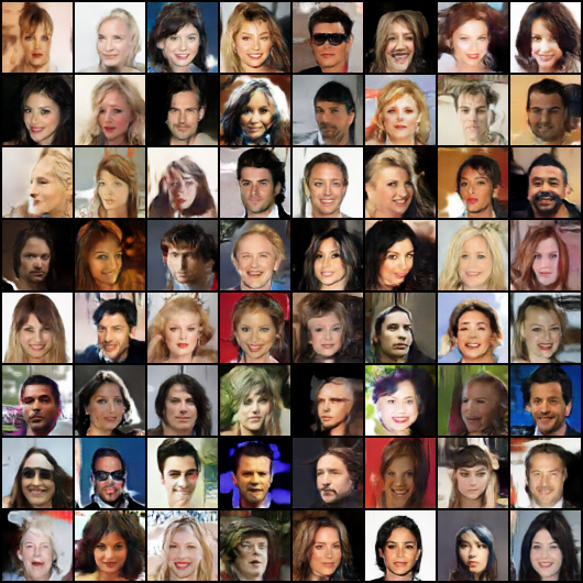
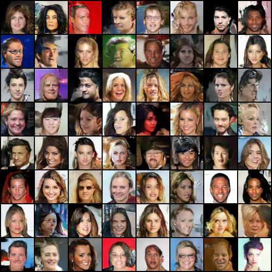
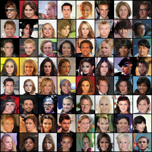
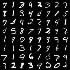
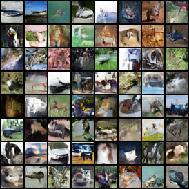
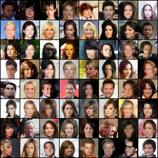
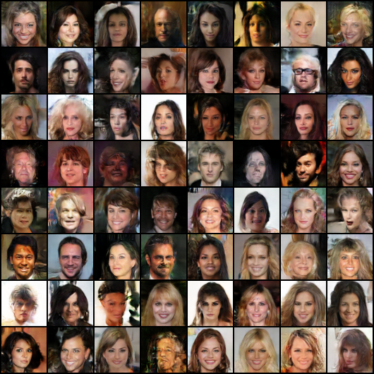
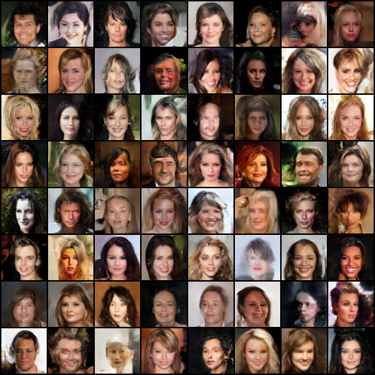
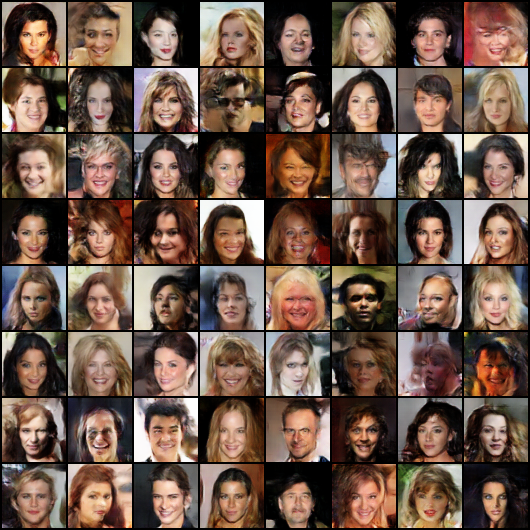
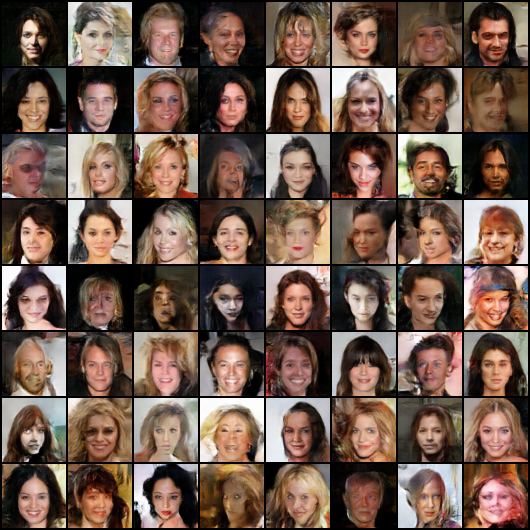
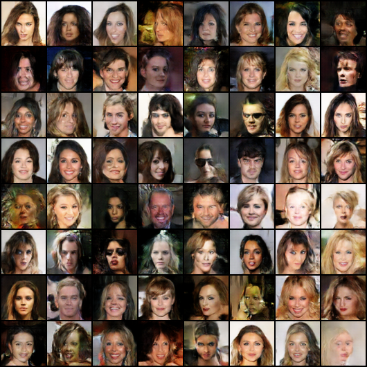
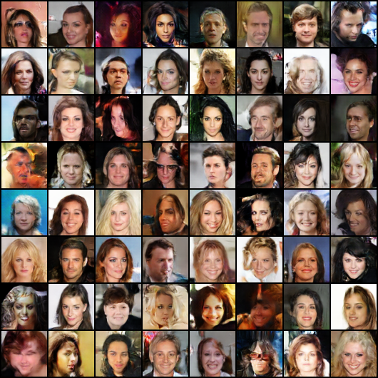
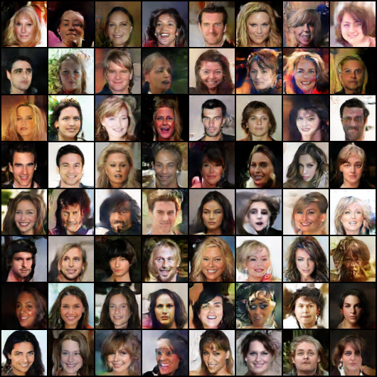
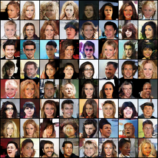
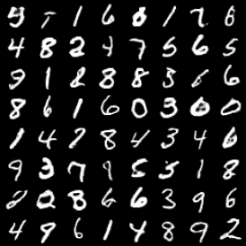
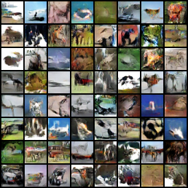
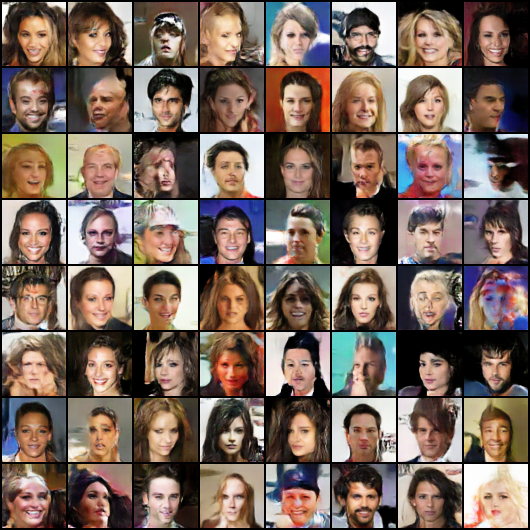
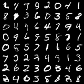
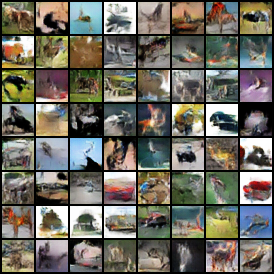
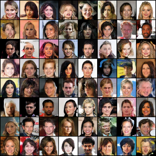
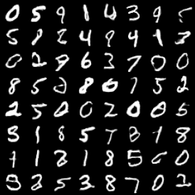
Figure 51 shows the sample images of WGAN-SN and some extremely degenerate loss functions, which corresponds to Table 5 in the main paper. It can be observed that all loss functions have similar performance.

Table 6: Network architectures. BN: batch normalization; SN: spectral normalization; GP: gradient penalty.
z100𝒩(0,1)𝑧superscript100similar-to𝒩01z\in\mathbb{R}^{100}\sim\mathcal{N}(0,1)
Reshape 1×1×100absent11100\to 1\times 1\times 100
4×4444\times 4, stride=1, deconv. BN 512 ReLU
4×4444\times 4, stride=2, deconv. BN 256 ReLU
4×4444\times 4, stride=2, deconv. BN 128 ReLU
4×4444\times 4, stride=2, deconv. BN 64 ReLU
4×4444\times 4, stride=2, deconv. 3 Tanh
(a) Generator
RGB image x[1,1]64×64×3𝑥superscript1164643x\in[-1,1]^{64\times 64\times 3}
4×4444\times 4, stride=2, conv 64 BN lReLU(0.2)
4×4444\times 4, stride=2, conv 128 BN lReLU(0.2)
4×4444\times 4, stride=2, conv 256 BN lReLU(0.2)
4×4444\times 4, stride=2, conv 512 BN lReLU(0.2)
4×4444\times 4, stride=1, conv 1
(b) Discriminator
(a) Network architectures with gradient penalty (GP) regularizer (64×64646464\times 64 resolution).
z100𝒩(0,1)𝑧superscript100similar-to𝒩01z\in\mathbb{R}^{100}\sim\mathcal{N}(0,1)
Reshape 1×1×100absent11100\to 1\times 1\times 100
4×4444\times 4, stride=1, deconv. BN 512 ReLU
4×4444\times 4, stride=2, deconv. BN 256 ReLU
4×4444\times 4, stride=2, deconv. BN 128 ReLU
4×4444\times 4, stride=2, deconv. BN 64 ReLU
4×4444\times 4, stride=2, deconv. 3 Tanh
(c) Generator
RGB image x[1,1]64×64×3𝑥superscript1164643x\in[-1,1]^{64\times 64\times 3}
4×4444\times 4, stride=2, conv 64 SN lReLU(0.2)
4×4444\times 4, stride=2, conv 128 SN lReLU(0.2)
4×4444\times 4, stride=2, conv 256 SN lReLU(0.2)
4×4444\times 4, stride=2, conv 512 SN lReLU(0.2)
4×4444\times 4, stride=1, conv 1
(d) Discriminator
(b) Network architectures with spectral normalization (SN) regularizer (64×64646464\times 64 resolution).
z100𝒩(0,1)𝑧superscript100similar-to𝒩01z\in\mathbb{R}^{100}\sim\mathcal{N}(0,1)
Reshape 1×1×100absent11100\to 1\times 1\times 100
4×4444\times 4, stride=1, deconv. BN 256 ReLU
4×4444\times 4, stride=2, deconv. BN 128 ReLU
4×4444\times 4, stride=2, deconv. BN 64 ReLU
4×4444\times 4, stride=2, deconv. 3 Tanh
(e) Generator
Image x[1,1]32×32×c𝑥superscript113232𝑐x\in[-1,1]^{32\times 32\times c}
4×4444\times 4, stride=2, conv 64 SN lReLU(0.2)
4×4444\times 4, stride=2, conv 128 SN lReLU(0.2)
4×4444\times 4, stride=2, conv 256 SN lReLU(0.2)
4×4444\times 4, stride=1, conv 1
(f) Discriminator
(c) Network architectures with spectral normalization (SN) regularizer (32×32323232\times 32 resolution). For input x[1,1]32×32×c𝑥superscript113232𝑐x\in[-1,1]^{32\times 32\times c}, c=3𝑐3c=3 for CIFAR10 dataset and c=1𝑐1c=1 for MNIST dataset.
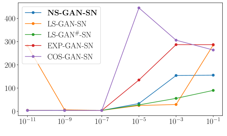
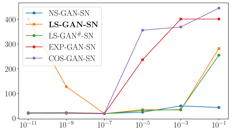
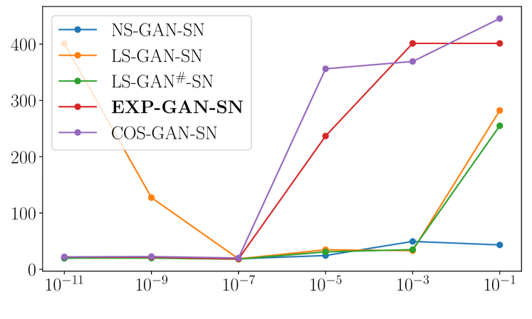
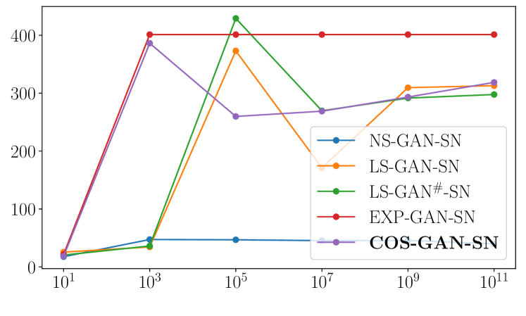
Table 7: FID scores v.s. α𝛼\alpha. For the line plots, the x𝑥x-axis shows α𝛼\alpha (in log scale) and the y𝑦y-axis shows the FID scores. Lower FID scores are better. The FID scores of the datasets in bold are not included in the main paper.
Dataset GANs FID Scores Line Plot
α𝛼\alpha = 1e111superscript𝑒111e^{-11} 1e91superscript𝑒91e^{-9} 1e71superscript𝑒71e^{-7} 1e51superscript𝑒51e^{-5} 1e31superscript𝑒31e^{-3} 1e11superscript𝑒11e^{-1}
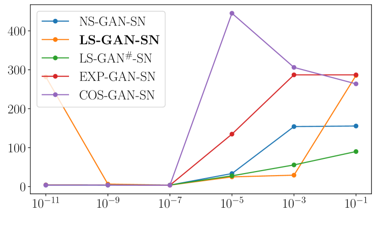
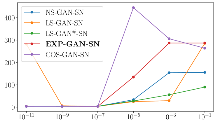
MNIST NS-GAN-SN 3.67 3.61 3.81 33.48 154.14 155.54 [Uncaptioned image]
LS-GAN-SN 281.82 6.48 3.74 24.93 29.31 285.46
LS-GAN#-SN 4.25 4.15 3.99 27.62 55.64 90.00
COS-GAN-SN 3.74 3.93 3.66 445.15 306.09 263.85
EXP-GAN-SN 4.14 4.01 3.54 134.76 286.96 286.96
CIFAR10 NS-GAN-SN 19.58 22.46 18.73 24.57 49.56 43.42 [Uncaptioned image]
LS-GAN-SN 400.91 127.38 18.68 34.78 33.17 282.11
LS-GAN#-SN 20.16 19.96 18.13 31.03 35.06 254.88
COS-GAN-SN 22.16 22.69 20.19 356.10 369.11 445.37
EXP-GAN-SN 21.93 21.70 18.50 236.77 401.24 401.24
CelebA NS-GAN-SN 9.08 7.05 7.84 18.51 18.41 242.64 [Uncaptioned image]
LS-GAN-SN 135.17 6.57 10.67 13.39 17.42 311.93
LS-GAN#-SN 6.66 5.68 8.72 11.13 14.90 383.61
COS-GAN-SN 8.00 6.31 300.55 280.84 373.31 318.53
EXP-GAN-SN 8.85 6.09 264.49 375.32 375.32 375.32
(a) kSN=50.0subscript𝑘𝑆𝑁50.0k_{SN}=50.0
Dataset GANs FID Scores Line Plot
α𝛼\alpha = 1e11superscript𝑒11e^{1} 1e31superscript𝑒31e^{3} 1e51superscript𝑒51e^{5} 1e71superscript𝑒71e^{7} 1e91superscript𝑒91e^{9} 1e111superscript𝑒111e^{11}
MNIST NS-GAN-SN 6.55 148.97 134.44 133.82 130.21 131.87 [Uncaptioned image]
LS-GAN-SN 23.37 26.96 260.05 255.73 256.96 265.76
LS-GAN#-SN 13.43 26.51 271.85 212.74 274.63 269.96
COS-GAN-SN 11.79 377.62 375.72 363.45 401.12 376.39
EXP-GAN-SN 11.02 286.96 286.96 286.96 286.96 286.96
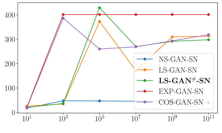
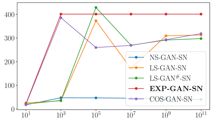
CIFAR10 NS-GAN-SN 17.63 47.31 46.85 45.44 45.67 39.90 [Uncaptioned image]
LS-GAN-SN 25.55 34.44 373.07 171.18 309.55 312.96
LS-GAN#-SN 20.45 36.18 429.21 269.63 291.55 297.71
COS-GAN-SN 18.59 386.24 259.83 268.89 293.29 318.65
EXP-GAN-SN 21.56 401.24 401.24 401.24 401.24 401.24
CelebA NS-GAN-SN 5.88 16.14 17.75 17.67 16.87 18.81 [Uncaptioned image]
LS-GAN-SN 8.41 12.09 201.22 312.83 299.30 321.84
LS-GAN#-SN 7.21 13.13 221.41 248.48 311.21 315.94
COS-GAN-SN 6.62 450.57 233.42 390.40 306.17 335.87
EXP-GAN-SN 6.91 375.32 375.32 375.32 375.32 375.32
(b) kSN=1.0subscript𝑘𝑆𝑁1.0k_{SN}=1.0
Table 8: Inception Scores (IS) v.s. α𝛼\alpha on CIFAR10. Higher IS are better.
GANs Inception Scores
α𝛼\alpha = 1e91superscript𝑒91e^{-9} 1e71superscript𝑒71e^{-7} 1e51superscript𝑒51e^{-5} 1e31superscript𝑒31e^{-3} 1e11superscript𝑒11e^{-1} 1e01superscript𝑒01e^{0} 1e11superscript𝑒11e^{1} 1e31superscript𝑒31e^{3} 1e51superscript𝑒51e^{5} 1e71superscript𝑒71e^{7} 1e91superscript𝑒91e^{9}
NS-GAN 4.32 4.04 4.03 4.00 4.47 4.48 4.64 3.60 3.23 3.31 3.49
LS-GAN 1.00 1.00 1.46 2.13 4.36 4.30 4.19 3.66 1.02 1.00 1.33
LS-GAN# 3.95 4.13 4.28 4.28 4.37 4.36 4.40 3.91 1.04 1.30 1.03
EXP-GAN 4.20 4.01 3.97 4.24 4.34 4.31 4.30 1.00 1.00 1.00 1.00
COS-GAN 4.20 4.10 4.24 4.13 4.32 4.35 4.40 2.00 1.00 1.05 1.35
(a) Lipschitz regularizer: SN
GANs Inception Scores
α𝛼\alpha = 1e91superscript𝑒91e^{-9} 1e71superscript𝑒71e^{-7} 1e51superscript𝑒51e^{-5} 1e31superscript𝑒31e^{-3} 1e11superscript𝑒11e^{-1} 1e01superscript𝑒01e^{0} 1e11superscript𝑒11e^{1} 1e31superscript𝑒31e^{3} 1e51superscript𝑒51e^{5} 1e71superscript𝑒71e^{7} 1e91superscript𝑒91e^{9}
NS-GAN 3.80 4.03 4.00 4.29 4.37 4.29 4.48 3.36 3.51 3.55 3.52
LS-GAN 1.00 1.00 1.53 2.24 4.37 4.59 4.25 3.60 1.21 1.37 1.27
LS-GAN# 4.05 3.88 3.91 4.02 4.31 4.54 4.44 3.92 1.64 1.32 1.00
EXP-GAN 3.99 3.94 3.98 4.22 4.42 4.34 4.43 1.00 1.00 1.00 1.00
COS-GAN 3.98 4.21 3.98 3.71 4.25 4.60 4.43 1.04 1.61 1.29 1.66
(b) Lipschitz regularizer: SRN+SN
Table 9: Neural Divergence (ND) v.s. α𝛼\alpha on CIFAR10. Lower ND are better.
GANs Neural Divergence
α𝛼\alpha = 1e91superscript𝑒91e^{-9} 1e71superscript𝑒71e^{-7} 1e51superscript𝑒51e^{-5} 1e31superscript𝑒31e^{-3} 1e11superscript𝑒11e^{-1} 1e01superscript𝑒01e^{0} 1e11superscript𝑒11e^{1} 1e31superscript𝑒31e^{3} 1e51superscript𝑒51e^{5} 1e71superscript𝑒71e^{7} 1e91superscript𝑒91e^{9}
NS-GAN 44.76 36.04 39.01 37.31 36.39 32.98 24.47 52.44 46.27 52.33 51.26
LS-GAN 157.69 222.71 82.76 118.53 37.16 25.94 42.15 38.47 72.27 155.82 286.46
LS-GAN# 36.71 35.07 40.61 43.93 32.97 28.01 32.62 41.48 72.47 259.10 167.50
EXP-GAN 36.22 43.71 41.67 35.37 34.23 32.49 31.79 nan nan nan nan
COS-GAN 40.53 35.66 36.33 39.48 36.39 31.73 33.21 477.07 61.40 69.79 81.15
(a) Lipschitz regularizer: SN
GANs Neural Divergence
α𝛼\alpha = 1e91superscript𝑒91e^{-9} 1e71superscript𝑒71e^{-7} 1e51superscript𝑒51e^{-5} 1e31superscript𝑒31e^{-3} 1e11superscript𝑒11e^{-1} 1e01superscript𝑒01e^{0} 1e11superscript𝑒11e^{1} 1e31superscript𝑒31e^{3} 1e51superscript𝑒51e^{5} 1e71superscript𝑒71e^{7} 1e91superscript𝑒91e^{9}
NS-GAN 39.28 37.12 31.60 37.82 33.56 23.33 26.57 34.30 49.68 45.96 52.72
LS-GAN 149.16 144.51 75.44 106.35 32.28 26.55 31.18 35.09 81.23 314.82 273.76
LS-GAN# 45.73 36.29 41.87 39.78 22.94 28.94 28.52 42.42 60.87 240.42 142.73
EXP-GAN 38.78 39.59 31.07 33.98 27.61 29.34 24.56 nan nan nan nan
COS-GAN 35.85 40.54 31.28 41.60 30.50 39.72 25.62 104.24 107.67 263.35 158.75
(b) Lipschitz regularizer: SRN+SN
FID scores v.s. kSNsubscript𝑘𝑆𝑁k_{SN} of Different Loss Functions
- MNIST -
Refer to caption
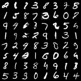
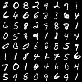
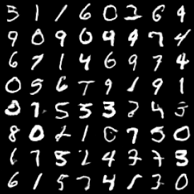
(a) kSNsubscript𝑘𝑆𝑁k_{SN}=50.0, FIDFID\mathrm{FID}=155.41
Refer to caption
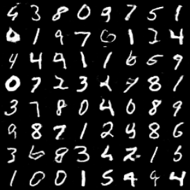
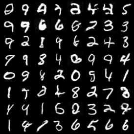
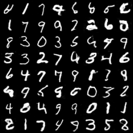
(b) kSNsubscript𝑘𝑆𝑁k_{SN}=10.0, FIDFID\mathrm{FID}=156.60
Refer to caption
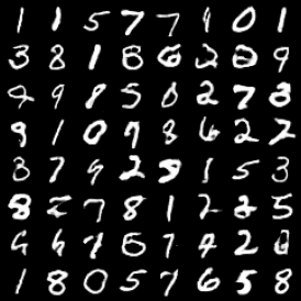
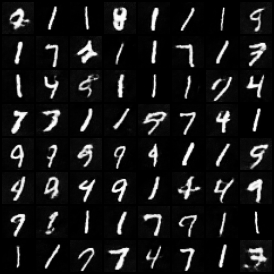
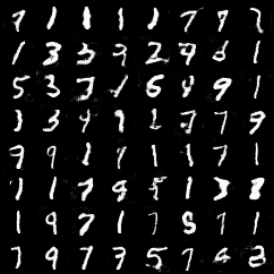
(c) kSNsubscript𝑘𝑆𝑁k_{SN}=5.0, FIDFID\mathrm{FID}=144.28
Refer to caption
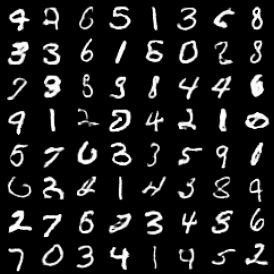
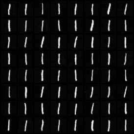
(d) kSNsubscript𝑘𝑆𝑁k_{SN}=1.0, FIDFID\mathrm{FID}=3.90
Refer to caption
(e) kSNsubscript𝑘𝑆𝑁k_{SN}=0.5, FIDFID\mathrm{FID}=4.20
Refer to caption
(f) kSNsubscript𝑘𝑆𝑁k_{SN}=0.25, FIDFID\mathrm{FID}=3.99
Refer to caption
(g) kSNsubscript𝑘𝑆𝑁k_{SN}=0.2, FIDFID\mathrm{FID}=5.41
Refer to caption
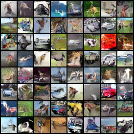
Figure 6: Samples of randomly generated images with NS-GAN-SN of varying kSNsubscript𝑘𝑆𝑁k_{SN} (MNIST). For the line plot, x𝑥x-axis shows kSNsubscript𝑘𝑆𝑁k_{SN} (in log scale) and y𝑦y-axis shows the FID scores.
Refer to caption
(a) kSNsubscript𝑘𝑆𝑁k_{SN}=50.0, FIDFID\mathrm{FID}=309.35
Refer to caption
(b) kSNsubscript𝑘𝑆𝑁k_{SN}=10.0, FIDFID\mathrm{FID}=59.04
Refer to caption
(c) kSNsubscript𝑘𝑆𝑁k_{SN}=5.0, FIDFID\mathrm{FID}=36.26
Refer to caption
(d) kSNsubscript𝑘𝑆𝑁k_{SN}=1.0, FIDFID\mathrm{FID}=4.42
Refer to caption
(e) kSNsubscript𝑘𝑆𝑁k_{SN}=0.5, FIDFID\mathrm{FID}=3.90
Refer to caption
(f) kSNsubscript𝑘𝑆𝑁k_{SN}=0.25, FIDFID\mathrm{FID}=3.96
Refer to caption
(g) kSNsubscript𝑘𝑆𝑁k_{SN}=0.2, FIDFID\mathrm{FID}=5.14
Refer to caption
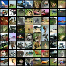
Figure 7: Samples of randomly generated images with LS-GAN-SN of varying kSNsubscript𝑘𝑆𝑁k_{SN} (MNIST). For the line plot, x𝑥x-axis shows kSNsubscript𝑘𝑆𝑁k_{SN} (in log scale) and y𝑦y-axis shows the FID scores.
Refer to caption
(a) kSN=50.0subscript𝑘𝑆𝑁50.0k_{SN}=50.0, FID=3.71FID3.71\mathrm{FID}=3.71
Refer to caption
(b) kSN=10.0subscript𝑘𝑆𝑁10.0k_{SN}=10.0, FID=3.50FID3.50\mathrm{FID}=3.50
Refer to caption
(c) kSN=5.0subscript𝑘𝑆𝑁5.0k_{SN}=5.0, FID=3.58FID3.58\mathrm{FID}=3.58
Refer to caption
(d) kSN=1.0subscript𝑘𝑆𝑁1.0k_{SN}=1.0, FID=4.70FID4.70\mathrm{FID}=4.70
Refer to caption
(e) kSN=0.5subscript𝑘𝑆𝑁0.5k_{SN}=0.5, FID=4.44FID4.44\mathrm{FID}=4.44
Refer to caption
(f) kSN=0.25subscript𝑘𝑆𝑁0.25k_{SN}=0.25, FID=6.06FID6.06\mathrm{FID}=6.06
Refer to caption
(g) kSN=0.2subscript𝑘𝑆𝑁0.2k_{SN}=0.2, FID=6.35FID6.35\mathrm{FID}=6.35
Refer to caption
Figure 8: Samples of randomly generated images with WGAN-SN of varying kSNsubscript𝑘𝑆𝑁k_{SN} (MNIST). For the line plot, x𝑥x-axis shows kSNsubscript𝑘𝑆𝑁k_{SN} (in log scale) and y𝑦y-axis shows the FID scores.
Refer to caption
(a) kSNsubscript𝑘𝑆𝑁k_{SN}=50.0, FIDFID\mathrm{FID}=287.23
Refer to caption
(b) kSNsubscript𝑘𝑆𝑁k_{SN}=10.0, FIDFID\mathrm{FID}=426.62
Refer to caption
(c) kSNsubscript𝑘𝑆𝑁k_{SN}=5.0, FIDFID\mathrm{FID}=291.44
Refer to caption
(d) kSNsubscript𝑘𝑆𝑁k_{SN}=1.0, FIDFID\mathrm{FID}=3.86
Refer to caption
(e) kSNsubscript𝑘𝑆𝑁k_{SN}=0.5, FIDFID\mathrm{FID}=4.05
Refer to caption
(f) kSNsubscript𝑘𝑆𝑁k_{SN}=0.25, FIDFID\mathrm{FID}=4.83
Refer to caption
(g) kSNsubscript𝑘𝑆𝑁k_{SN}=0.2, FIDFID\mathrm{FID}=5.41
Refer to caption
Figure 9: Samples of randomly generated images with COS-GAN-SN of varying kSNsubscript𝑘𝑆𝑁k_{SN} (MNIST). For the line plot, x𝑥x-axis shows kSNsubscript𝑘𝑆𝑁k_{SN} (in log scale) and y𝑦y-axis shows the FID scores.
Refer to caption
(a) kSNsubscript𝑘𝑆𝑁k_{SN}=50.0, FIDFID\mathrm{FID}=286.96
Refer to caption
(b) kSNsubscript𝑘𝑆𝑁k_{SN}=10.0, FIDFID\mathrm{FID}=286.96
Refer to caption
(c) kSNsubscript𝑘𝑆𝑁k_{SN}=5.0, FIDFID\mathrm{FID}=286.96
Refer to caption
(d) kSNsubscript𝑘𝑆𝑁k_{SN}=1.0, FIDFID\mathrm{FID}=3.69
Refer to caption
(e) kSNsubscript𝑘𝑆𝑁k_{SN}=0.5, FIDFID\mathrm{FID}=4.25
Refer to caption
(f) kSNsubscript𝑘𝑆𝑁k_{SN}=0.25, FIDFID\mathrm{FID}=4.93
Refer to caption
(g) kSNsubscript𝑘𝑆𝑁k_{SN}=0.2, FIDFID\mathrm{FID}=4.38
Refer to caption
Figure 10: Samples of randomly generated images with EXP-GAN-SN of varying kSNsubscript𝑘𝑆𝑁k_{SN} (MNIST). For the line plot, x𝑥x-axis shows kSNsubscript𝑘𝑆𝑁k_{SN} (in log scale) and y𝑦y-axis shows the FID scores.
FID scores v.s. kSNsubscript𝑘𝑆𝑁k_{SN} of Different Loss Functions
- CIFAR10 -
Refer to caption
(a) kSNsubscript𝑘𝑆𝑁k_{SN}=50.0, FIDFID\mathrm{FID}=48.03
Refer to caption
(b) kSNsubscript𝑘𝑆𝑁k_{SN}=10.0, FIDFID\mathrm{FID}=49.67
Refer to caption
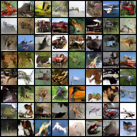
(c) kSNsubscript𝑘𝑆𝑁k_{SN}=5.0, FIDFID\mathrm{FID}=41.04
Refer to caption
(d) kSNsubscript𝑘𝑆𝑁k_{SN}=1.0, FIDFID\mathrm{FID}=15.81
Refer to caption
(e) kSNsubscript𝑘𝑆𝑁k_{SN}=0.5, FIDFID\mathrm{FID}=23.29
Refer to caption
(f) kSNsubscript𝑘𝑆𝑁k_{SN}=0.25, FIDFID\mathrm{FID}=24.37
Refer to caption
(g) kSNsubscript𝑘𝑆𝑁k_{SN}=0.2, FIDFID\mathrm{FID}=29.23
Refer to caption
Figure 11: Samples of randomly generated images with NS-GAN-SN of varying kSNsubscript𝑘𝑆𝑁k_{SN} (CIFAR10). For the line plot, x𝑥x-axis shows kSNsubscript𝑘𝑆𝑁k_{SN} (in log scale) and y𝑦y-axis shows the FID scores.
Refer to caption
(a) kSNsubscript𝑘𝑆𝑁k_{SN}=50.0, FIDFID\mathrm{FID}= 349.35
Refer to caption
(b) kSNsubscript𝑘𝑆𝑁k_{SN}=10.0, FIDFID\mathrm{FID}= 39.90
Refer to caption
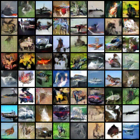
(c) kSNsubscript𝑘𝑆𝑁k_{SN}=5.0, FIDFID\mathrm{FID}= 33.53
Refer to caption
(d) kSNsubscript𝑘𝑆𝑁k_{SN}=1.0, FIDFID\mathrm{FID}= 17.30
Refer to caption
(e) kSNsubscript𝑘𝑆𝑁k_{SN}=0.5, FIDFID\mathrm{FID}= 23.14
Refer to caption
(f) kSNsubscript𝑘𝑆𝑁k_{SN}=0.25, FIDFID\mathrm{FID}= 26.85
Refer to caption
(g) kSNsubscript𝑘𝑆𝑁k_{SN}=0.2, FIDFID\mathrm{FID}= 28.04
Refer to caption
Figure 12: Samples of randomly generated images with LS-GAN-SN of varying kSNsubscript𝑘𝑆𝑁k_{SN} (CIFAR10). For the line plot, x𝑥x-axis shows kSNsubscript𝑘𝑆𝑁k_{SN} (in log scale) and y𝑦y-axis shows the FID scores.
Refer to caption
(a) kSNsubscript𝑘𝑆𝑁k_{SN}=50.0, FIDFID\mathrm{FID}= 23.36
Refer to caption
(b) kSNsubscript𝑘𝑆𝑁k_{SN}=10.0, FIDFID\mathrm{FID}= 21.45
Refer to caption
(c) kSNsubscript𝑘𝑆𝑁k_{SN}=5.0, FIDFID\mathrm{FID}= 21.63
Refer to caption
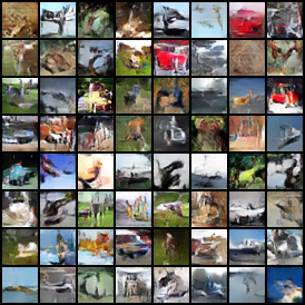
(d) kSNsubscript𝑘𝑆𝑁k_{SN}=1.0, FIDFID\mathrm{FID}= 21.75
Refer to caption
(e) kSNsubscript𝑘𝑆𝑁k_{SN}=0.5, FIDFID\mathrm{FID}= 26.61
Refer to caption
(f) kSNsubscript𝑘𝑆𝑁k_{SN}=0.25, FIDFID\mathrm{FID}= 25.07
Refer to caption
(g) kSNsubscript𝑘𝑆𝑁k_{SN}=0.2, FIDFID\mathrm{FID}= 29.20
Refer to caption
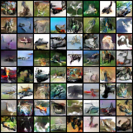
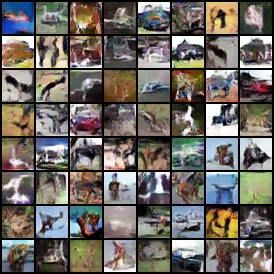
Figure 13: Samples of randomly generated images with WGAN-SN of varying kSNsubscript𝑘𝑆𝑁k_{SN} (CIFAR10). For the line plot, x𝑥x-axis shows kSNsubscript𝑘𝑆𝑁k_{SN} (in log scale) and y𝑦y-axis shows the FID scores.
Refer to caption
(a) kSNsubscript𝑘𝑆𝑁k_{SN}=50.0, FIDFID\mathrm{FID}= 370.13
Refer to caption
(b) kSNsubscript𝑘𝑆𝑁k_{SN}=10.0, FIDFID\mathrm{FID}= 327.20
Refer to caption
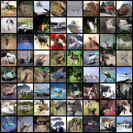
(c) kSNsubscript𝑘𝑆𝑁k_{SN}=5.0, FIDFID\mathrm{FID}= 309.96
Refer to caption
(d) kSNsubscript𝑘𝑆𝑁k_{SN}=1.0, FIDFID\mathrm{FID}= 15.88
Refer to caption
(e) kSNsubscript𝑘𝑆𝑁k_{SN}=0.5, FIDFID\mathrm{FID}= 20.73
Refer to caption
(f) kSNsubscript𝑘𝑆𝑁k_{SN}=0.25, FIDFID\mathrm{FID}= 25.31
Refer to caption
(g) kSNsubscript𝑘𝑆𝑁k_{SN}=0.2, FIDFID\mathrm{FID}= 29.45
Refer to caption
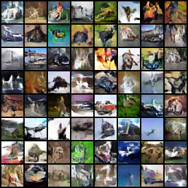
Figure 14: Samples of randomly generated images with COS-GAN-SN of varying kSNsubscript𝑘𝑆𝑁k_{SN} (CIFAR10). For the line plot, x𝑥x-axis shows kSNsubscript𝑘𝑆𝑁k_{SN} (in log scale) and y𝑦y-axis shows the FID scores.
Refer to caption
(a) kSNsubscript𝑘𝑆𝑁k_{SN}=50.0, FIDFID\mathrm{FID}= 401.24
Refer to caption
(b) kSNsubscript𝑘𝑆𝑁k_{SN}=10.0, FIDFID\mathrm{FID}= 401.24
Refer to caption
(c) kSNsubscript𝑘𝑆𝑁k_{SN}=5.0, FIDFID\mathrm{FID}= 401.24
Refer to caption
(d) kSNsubscript𝑘𝑆𝑁k_{SN}=1.0, FIDFID\mathrm{FID}= 16.66
Refer to caption
(e) kSNsubscript𝑘𝑆𝑁k_{SN}=0.5, FIDFID\mathrm{FID}= 20.90
Refer to caption
(f) kSNsubscript𝑘𝑆𝑁k_{SN}=0.25, FIDFID\mathrm{FID}= 24.74
Refer to caption
(g) kSNsubscript𝑘𝑆𝑁k_{SN}=0.2, FIDFID\mathrm{FID}= 30.89
Refer to caption
Figure 15: Samples of randomly generated images with EXP-GAN-SN of varying kSNsubscript𝑘𝑆𝑁k_{SN} (CIFAR10). For the line plot, x𝑥x-axis shows kSNsubscript𝑘𝑆𝑁k_{SN} (in log scale) and y𝑦y-axis shows the FID scores.
FID scores v.s. kSNsubscript𝑘𝑆𝑁k_{SN} of Different Loss Functions
- CelebA -
Refer to caption
(a) kSNsubscript𝑘𝑆𝑁k_{SN}=50.0, FIDFID\mathrm{FID}= 184.06
Refer to caption
(b) kSNsubscript𝑘𝑆𝑁k_{SN}=10.0, FIDFID\mathrm{FID}= 17.04
Refer to caption
(c) kSNsubscript𝑘𝑆𝑁k_{SN}=5.0, FIDFID\mathrm{FID}= 18.95
Refer to caption
(d) kSNsubscript𝑘𝑆𝑁k_{SN}=1.0, FIDFID\mathrm{FID}= 6.11
Refer to caption
(e) kSNsubscript𝑘𝑆𝑁k_{SN}=0.5, FIDFID\mathrm{FID}= 8.04
Refer to caption
(f) kSNsubscript𝑘𝑆𝑁k_{SN}=0.25, FIDFID\mathrm{FID}= 12.71
Refer to caption
(g) kSNsubscript𝑘𝑆𝑁k_{SN}=0.2, FIDFID\mathrm{FID}= 18.59
Refer to caption
Figure 16: Samples of randomly generated images with NS-GAN-SN of varying kSNsubscript𝑘𝑆𝑁k_{SN} (CelebA). For the line plot, x𝑥x-axis shows kSNsubscript𝑘𝑆𝑁k_{SN} (in log scale) and y𝑦y-axis shows the FID scores.
Refer to caption
(a) kSNsubscript𝑘𝑆𝑁k_{SN}=50.0, FIDFID\mathrm{FID}= 399.39
Refer to caption
(b) kSNsubscript𝑘𝑆𝑁k_{SN}=10.0, FIDFID\mathrm{FID}= 13.14
Refer to caption
(c) kSNsubscript𝑘𝑆𝑁k_{SN}=5.0, FIDFID\mathrm{FID}= 12.40
Refer to caption
(d) kSNsubscript𝑘𝑆𝑁k_{SN}=1.0, FIDFID\mathrm{FID}= 5.69
Refer to caption
(e) kSNsubscript𝑘𝑆𝑁k_{SN}=0.5, FIDFID\mathrm{FID}= 8.85
Refer to caption
(f) kSNsubscript𝑘𝑆𝑁k_{SN}=0.25, FIDFID\mathrm{FID}= 12.14
Refer to caption
(g) kSNsubscript𝑘𝑆𝑁k_{SN}=0.2, FIDFID\mathrm{FID}= 20.34
Refer to caption
Figure 17: Samples of randomly generated images with LS-GAN-SN of varying kSNsubscript𝑘𝑆𝑁k_{SN} (CelebA). For the line plot, x𝑥x-axis shows kSNsubscript𝑘𝑆𝑁k_{SN} (in log scale) and y𝑦y-axis shows the FID scores.
Refer to caption
(a) kSNsubscript𝑘𝑆𝑁k_{SN}=50.0, FIDFID\mathrm{FID}= 7.82
Refer to caption
(b) kSNsubscript𝑘𝑆𝑁k_{SN}=10.0, FIDFID\mathrm{FID}= 7.37
Refer to caption
(c) kSNsubscript𝑘𝑆𝑁k_{SN}=5.0, FIDFID\mathrm{FID}= 9.03
Refer to caption
(d) kSNsubscript𝑘𝑆𝑁k_{SN}=1.0, FIDFID\mathrm{FID}= 9.41
Refer to caption
(e) kSNsubscript𝑘𝑆𝑁k_{SN}=0.5, FIDFID\mathrm{FID}= 8.48
Refer to caption
(f) kSNsubscript𝑘𝑆𝑁k_{SN}=0.25, FIDFID\mathrm{FID}= 17.93
Refer to caption
(g) kSNsubscript𝑘𝑆𝑁k_{SN}=0.2, FIDFID\mathrm{FID}= 23.26
Refer to caption
Figure 18: Samples of randomly generated images with WGAN-SN of varying kSNsubscript𝑘𝑆𝑁k_{SN} (CelebA). For the line plot, x𝑥x-axis shows kSNsubscript𝑘𝑆𝑁k_{SN} (in log scale) and y𝑦y-axis shows the FID scores.
Refer to caption
(a) kSNsubscript𝑘𝑆𝑁k_{SN}=50.0, FIDFID\mathrm{FID}= 256.44
Refer to caption
(b) kSNsubscript𝑘𝑆𝑁k_{SN}=10.0, FIDFID\mathrm{FID}= 265.53
Refer to caption
(c) kSNsubscript𝑘𝑆𝑁k_{SN}=5.0, FIDFID\mathrm{FID}= 356.70
Refer to caption
(d) kSNsubscript𝑘𝑆𝑁k_{SN}=1.0, FIDFID\mathrm{FID}= 5.20
Refer to caption
(e) kSNsubscript𝑘𝑆𝑁k_{SN}=0.5, FIDFID\mathrm{FID}= 8.88
Refer to caption
(f) kSNsubscript𝑘𝑆𝑁k_{SN}=0.25, FIDFID\mathrm{FID}= 13.93
Refer to caption
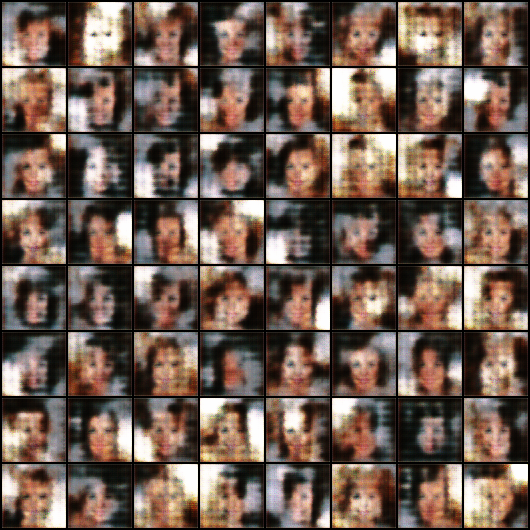
(g) kSNsubscript𝑘𝑆𝑁k_{SN}=0.2, FIDFID\mathrm{FID}= 20.59
Refer to caption
Figure 19: Samples of randomly generated images with COS-GAN-SN of varying kSNsubscript𝑘𝑆𝑁k_{SN} (CelebA). For the line plot, x𝑥x-axis shows kSNsubscript𝑘𝑆𝑁k_{SN} (in log scale) and y𝑦y-axis shows the FID scores.
Refer to caption
(a) kSNsubscript𝑘𝑆𝑁k_{SN}=50.0, FIDFID\mathrm{FID}= 328.94
Refer to caption
(b) kSNsubscript𝑘𝑆𝑁k_{SN}=10.0, FIDFID\mathrm{FID}= 328.94
Refer to caption
(c) kSNsubscript𝑘𝑆𝑁k_{SN}=5.0, FIDFID\mathrm{FID}= 328.94
Refer to caption
(d) kSNsubscript𝑘𝑆𝑁k_{SN}=1.0, FIDFID\mathrm{FID}= 5.88
Refer to caption
(e) kSNsubscript𝑘𝑆𝑁k_{SN}=0.5, FIDFID\mathrm{FID}= 9.18
Refer to caption
(f) kSNsubscript𝑘𝑆𝑁k_{SN}=0.25, FIDFID\mathrm{FID}= 13.65
Refer to caption
(g) kSNsubscript𝑘𝑆𝑁k_{SN}=0.2, FIDFID\mathrm{FID}= 18.23
Refer to caption
Figure 20: Samples of randomly generated images with EXP-GAN-SN of varying kSNsubscript𝑘𝑆𝑁k_{SN} (CelebA). For the line plot, x𝑥x-axis shows kSNsubscript𝑘𝑆𝑁k_{SN} (in log scale) and y𝑦y-axis shows the FID scores.
FID scores v.s. α𝛼\alpha (kSN=50.0subscript𝑘𝑆𝑁50.0k_{SN}=50.0) of Different Loss Functions
- MNIST -
Refer to caption
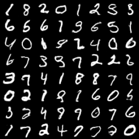
(a) α=1e11𝛼1superscript𝑒11\alpha=1e^{-11}, FID=3.67FID3.67\mathrm{FID}=3.67
Refer to caption
(b) α=1e9𝛼1superscript𝑒9\alpha=1e^{-9}, FID=3.61FID3.61\mathrm{FID}=3.61
Refer to caption
(c) α=1e7𝛼1superscript𝑒7\alpha=1e^{-7}, FID=3.81FID3.81\mathrm{FID}=3.81
Refer to caption
(d) α=1e5𝛼1superscript𝑒5\alpha=1e^{-5}, FID=33.48FID33.48\mathrm{FID}=33.48
Refer to caption
(e) α=1e3𝛼1superscript𝑒3\alpha=1e^{-3}, FID=154.14FID154.14\mathrm{FID}=154.14
Refer to caption
(f) α=1e1𝛼1superscript𝑒1\alpha=1e^{-1}, FID=155.54FID155.54\mathrm{FID}=155.54
Refer to caption
Figure 21: Samples of randomly generated images with NS-GAN-SN of varying α𝛼\alpha (kSN=50.0subscript𝑘𝑆𝑁50.0k_{SN}=50.0, MNIST). For the line plot, x𝑥x-axis shows α𝛼\alpha (in log scale) and y𝑦y-axis shows the FID scores.
Refer to caption
(a) α=1e11𝛼1superscript𝑒11\alpha=1e^{-11}, FIDFID\mathrm{FID}=281.82
Refer to caption
(b) α=1e9𝛼1superscript𝑒9\alpha=1e^{-9}, FID=6.48FID6.48\mathrm{FID}=6.48
Refer to caption
(c) α=1e7𝛼1superscript𝑒7\alpha=1e^{-7}, FID=3.74FID3.74\mathrm{FID}=3.74
Refer to caption
(d) α=1e5𝛼1superscript𝑒5\alpha=1e^{-5}, FID=24.93FID24.93\mathrm{FID}=24.93
Refer to caption
(e) α=1e3𝛼1superscript𝑒3\alpha=1e^{-3}, FID=29.31FID29.31\mathrm{FID}=29.31
Refer to caption
(f) α=1e1𝛼1superscript𝑒1\alpha=1e^{-1}, FID=285.46FID285.46\mathrm{FID}=285.46
Refer to caption
Figure 22: Samples of randomly generated images with LS-GAN-SN of varying α𝛼\alpha (kSN=50.0subscript𝑘𝑆𝑁50.0k_{SN}=50.0, MNIST). For the line plot, x𝑥x-axis shows α𝛼\alpha (in log scale) and y𝑦y-axis shows the FID scores.
Refer to caption
(a) α=1e11𝛼1superscript𝑒11\alpha=1e^{-11}, FID=4.25FID4.25\mathrm{FID}=4.25
Refer to caption
(b) α=1e9𝛼1superscript𝑒9\alpha=1e^{-9}, FID=4.15FID4.15\mathrm{FID}=4.15
Refer to caption
(c) α=1e7𝛼1superscript𝑒7\alpha=1e^{-7}, FID=3.99FID3.99\mathrm{FID}=3.99
Refer to caption
(d) α=1e5𝛼1superscript𝑒5\alpha=1e^{-5}, FID=27.62FID27.62\mathrm{FID}=27.62
Refer to caption
(e) α=1e3𝛼1superscript𝑒3\alpha=1e^{-3}, FID=55.64FID55.64\mathrm{FID}=55.64
Refer to caption
(f) α=1e1𝛼1superscript𝑒1\alpha=1e^{-1}, FID=90.00FID90.00\mathrm{FID}=90.00
Refer to caption
Figure 23: Samples of randomly generated images with LS-GAN#-SN of varying α𝛼\alpha (kSN=50.0subscript𝑘𝑆𝑁50.0k_{SN}=50.0, MNIST). For the line plot, x𝑥x-axis shows α𝛼\alpha (in log scale) and y𝑦y-axis shows the FID scores.
Refer to caption
(a) α=1e11𝛼1superscript𝑒11\alpha=1e^{-11}, FID=4.14FID4.14\mathrm{FID}=4.14
Refer to caption
(b) α=1e9𝛼1superscript𝑒9\alpha=1e^{-9}, FID=4.01FID4.01\mathrm{FID}=4.01
Refer to caption
(c) α=1e7𝛼1superscript𝑒7\alpha=1e^{-7}, FID=3.54FID3.54\mathrm{FID}=3.54
Refer to caption
(d) α=1e5𝛼1superscript𝑒5\alpha=1e^{-5}, FID=134.76FID134.76\mathrm{FID}=134.76
Refer to caption
(e) α=1e3𝛼1superscript𝑒3\alpha=1e^{-3}, FID=286.96FID286.96\mathrm{FID}=286.96
Refer to caption
(f) α=1e1𝛼1superscript𝑒1\alpha=1e^{-1}, FID=286.96FID286.96\mathrm{FID}=286.96
Refer to caption
Figure 24: Samples of randomly generated images with EXP-GAN-SN of varying α𝛼\alpha (kSN=50.0subscript𝑘𝑆𝑁50.0k_{SN}=50.0, MNIST). For the line plot, x𝑥x-axis shows α𝛼\alpha (in log scale) and y𝑦y-axis shows the FID scores.
Refer to caption
(a) α=1e11𝛼1superscript𝑒11\alpha=1e^{-11}, FID=3.74FID3.74\mathrm{FID}=3.74
Refer to caption
(b) α=1e9𝛼1superscript𝑒9\alpha=1e^{-9}, FID=3.93FID3.93\mathrm{FID}=3.93
Refer to caption
(c) α=1e7𝛼1superscript𝑒7\alpha=1e^{-7}, FID=3.66FID3.66\mathrm{FID}=3.66
Refer to caption
(d) α=1e5𝛼1superscript𝑒5\alpha=1e^{-5}, FID=445.15FID445.15\mathrm{FID}=445.15
Refer to caption
(e) α=1e3𝛼1superscript𝑒3\alpha=1e^{-3}, FID=306.09FID306.09\mathrm{FID}=306.09
Refer to caption
(f) α=1e1𝛼1superscript𝑒1\alpha=1e^{-1}, FID=263.85FID263.85\mathrm{FID}=263.85
Refer to caption
Figure 25: Samples of randomly generated images with COS-GAN-SN of varying α𝛼\alpha (kSN=50.0subscript𝑘𝑆𝑁50.0k_{SN}=50.0, MNIST). For the line plot, x𝑥x-axis shows α𝛼\alpha (in log scale) and y𝑦y-axis shows the FID scores.
FID scores v.s. α𝛼\alpha (kSN=50.0subscript𝑘𝑆𝑁50.0k_{SN}=50.0) of Different Loss Functions
- CIFAR10 -
Refer to caption
(a) α=1e11𝛼1superscript𝑒11\alpha=1e^{-11}, FID=19.58FID19.58\mathrm{FID}=19.58
Refer to caption
(b) α=1e9𝛼1superscript𝑒9\alpha=1e^{-9}, FID=22.46FID22.46\mathrm{FID}=22.46
Refer to caption
(c) α=1e7𝛼1superscript𝑒7\alpha=1e^{-7}, FID=18.73FID18.73\mathrm{FID}=18.73
Refer to caption
(d) α=1e5𝛼1superscript𝑒5\alpha=1e^{-5}, FID=24.57FID24.57\mathrm{FID}=24.57
Refer to caption
(e) α=1e3𝛼1superscript𝑒3\alpha=1e^{-3}, FID=49.56FID49.56\mathrm{FID}=49.56
Refer to caption
(f) α=1e1𝛼1superscript𝑒1\alpha=1e^{-1}, FID=43.42FID43.42\mathrm{FID}=43.42
Refer to caption
Figure 26: Samples of randomly generated images with NS-GAN-SN of varying α𝛼\alpha (kSN=50.0subscript𝑘𝑆𝑁50.0k_{SN}=50.0, CIFAR10). For the line plot, x𝑥x-axis shows α𝛼\alpha (in log scale) and y𝑦y-axis shows the FID scores.
Refer to caption
(a) α=1e11𝛼1superscript𝑒11\alpha=1e^{-11}, FIDFID\mathrm{FID}=400.91
Refer to caption
(b) α=1e9𝛼1superscript𝑒9\alpha=1e^{-9}, FID=127.38FID127.38\mathrm{FID}=127.38
Refer to caption
(c) α=1e7𝛼1superscript𝑒7\alpha=1e^{-7}, FID=18.68FID18.68\mathrm{FID}=18.68
Refer to caption
(d) α=1e5𝛼1superscript𝑒5\alpha=1e^{-5}, FID=34.78FID34.78\mathrm{FID}=34.78
Refer to caption
(e) α=1e3𝛼1superscript𝑒3\alpha=1e^{-3}, FID=33.17FID33.17\mathrm{FID}=33.17
Refer to caption
(f) α=1e1𝛼1superscript𝑒1\alpha=1e^{-1}, FID=282.11FID282.11\mathrm{FID}=282.11
Refer to caption
Figure 27: Samples of randomly generated images with LS-GAN-SN of varying α𝛼\alpha (kSN=50.0subscript𝑘𝑆𝑁50.0k_{SN}=50.0, CIFAR10). For the line plot, x𝑥x-axis shows α𝛼\alpha (in log scale) and y𝑦y-axis shows the FID scores.
Refer to caption
(a) α=1e11𝛼1superscript𝑒11\alpha=1e^{-11}, FID=20.16FID20.16\mathrm{FID}=20.16
Refer to caption
(b) α=1e9𝛼1superscript𝑒9\alpha=1e^{-9}, FID=19.96FID19.96\mathrm{FID}=19.96
Refer to caption
(c) α=1e7𝛼1superscript𝑒7\alpha=1e^{-7}, FID=18.13FID18.13\mathrm{FID}=18.13
Refer to caption
(d) α=1e5𝛼1superscript𝑒5\alpha=1e^{-5}, FID=31.03FID31.03\mathrm{FID}=31.03
Refer to caption
(e) α=1e3𝛼1superscript𝑒3\alpha=1e^{-3}, FID=35.06FID35.06\mathrm{FID}=35.06
Refer to caption
(f) α=1e1𝛼1superscript𝑒1\alpha=1e^{-1}, FID=254.88FID254.88\mathrm{FID}=254.88
Refer to caption
Figure 28: Samples of randomly generated images with LS-GAN#-SN of varying α𝛼\alpha (kSN=50.0subscript𝑘𝑆𝑁50.0k_{SN}=50.0, CIFAR10). For the line plot, x𝑥x-axis shows α𝛼\alpha (in log scale) and y𝑦y-axis shows the FID scores.
Refer to caption
(a) α=1e11𝛼1superscript𝑒11\alpha=1e^{-11}, FID=21.93FID21.93\mathrm{FID}=21.93
Refer to caption
(b) α=1e9𝛼1superscript𝑒9\alpha=1e^{-9}, FID=21.70FID21.70\mathrm{FID}=21.70
Refer to caption
(c) α=1e7𝛼1superscript𝑒7\alpha=1e^{-7}, FID=18.50FID18.50\mathrm{FID}=18.50
Refer to caption
(d) α=1e5𝛼1superscript𝑒5\alpha=1e^{-5}, FID=236.77FID236.77\mathrm{FID}=236.77
Refer to caption
(e) α=1e3𝛼1superscript𝑒3\alpha=1e^{-3}, FID=401.24FID401.24\mathrm{FID}=401.24
Refer to caption
(f) α=1e1𝛼1superscript𝑒1\alpha=1e^{-1}, FID=401.24FID401.24\mathrm{FID}=401.24
Refer to caption
Figure 29: Samples of randomly generated images with EXP-GAN-SN of varying α𝛼\alpha (kSN=50.0subscript𝑘𝑆𝑁50.0k_{SN}=50.0, CIFAR10). For the line plot, x𝑥x-axis shows α𝛼\alpha (in log scale) and y𝑦y-axis shows the FID scores.
Refer to caption
(a) α=1e11𝛼1superscript𝑒11\alpha=1e^{-11}, FID=22.16FID22.16\mathrm{FID}=22.16
Refer to caption
(b) α=1e9𝛼1superscript𝑒9\alpha=1e^{-9}, FID=22.69FID22.69\mathrm{FID}=22.69
Refer to caption
(c) α=1e7𝛼1superscript𝑒7\alpha=1e^{-7}, FID=20.19FID20.19\mathrm{FID}=20.19
Refer to caption
(d) α=1e5𝛼1superscript𝑒5\alpha=1e^{-5}, FID=356.10FID356.10\mathrm{FID}=356.10
Refer to caption
(e) α=1e3𝛼1superscript𝑒3\alpha=1e^{-3}, FID=369.11FID369.11\mathrm{FID}=369.11
Refer to caption
(f) α=1e1𝛼1superscript𝑒1\alpha=1e^{-1}, FID=445.37FID445.37\mathrm{FID}=445.37
Refer to caption
Figure 30: Samples of randomly generated images with COS-GAN-SN of varying α𝛼\alpha (kSN=50.0subscript𝑘𝑆𝑁50.0k_{SN}=50.0, CIFAR10). For the line plot, x𝑥x-axis shows α𝛼\alpha (in log scale) and y𝑦y-axis shows the FID scores.
FID scores v.s. α𝛼\alpha (kSN=50.0subscript𝑘𝑆𝑁50.0k_{SN}=50.0) of Different Loss Functions
- CelebA -
Refer to caption
(a) α=1e11𝛼1superscript𝑒11\alpha=1e^{-11}, FID=9.08FID9.08\mathrm{FID}=9.08
Refer to caption
(b) α=1e9𝛼1superscript𝑒9\alpha=1e^{-9}, FID=7.05FID7.05\mathrm{FID}=7.05
Refer to caption
(c) α=1e7𝛼1superscript𝑒7\alpha=1e^{-7}, FID=7.84FID7.84\mathrm{FID}=7.84
Refer to caption
(d) α=1e5𝛼1superscript𝑒5\alpha=1e^{-5}, FID=18.51FID18.51\mathrm{FID}=18.51
Refer to caption
(e) α=1e3𝛼1superscript𝑒3\alpha=1e^{-3}, FID=18.41FID18.41\mathrm{FID}=18.41
Refer to caption
(f) α=1e1𝛼1superscript𝑒1\alpha=1e^{-1}, FID=242.64FID242.64\mathrm{FID}=242.64
Refer to caption
Figure 31: Samples of randomly generated images with NS-GAN-SN of varying α𝛼\alpha (kSN=50.0subscript𝑘𝑆𝑁50.0k_{SN}=50.0, CelebA). For the line plot, x𝑥x-axis shows α𝛼\alpha (in log scale) and y𝑦y-axis shows the FID scores.
Refer to caption
(a) α=1e11𝛼1superscript𝑒11\alpha=1e^{-11}, FIDFID\mathrm{FID}=135.17
Refer to caption
(b) α=1e9𝛼1superscript𝑒9\alpha=1e^{-9}, FID=6.57FID6.57\mathrm{FID}=6.57
Refer to caption
(c) α=1e7𝛼1superscript𝑒7\alpha=1e^{-7}, FID=10.67FID10.67\mathrm{FID}=10.67
Refer to caption
(d) α=1e5𝛼1superscript𝑒5\alpha=1e^{-5}, FID=13.39FID13.39\mathrm{FID}=13.39
Refer to caption
(e) α=1e3𝛼1superscript𝑒3\alpha=1e^{-3}, FID=17.42FID17.42\mathrm{FID}=17.42
Refer to caption
(f) α=1e1𝛼1superscript𝑒1\alpha=1e^{-1}, FID=311.93FID311.93\mathrm{FID}=311.93
Refer to caption
Figure 32: Samples of randomly generated images with LS-GAN-SN of varying α𝛼\alpha (kSN=50.0subscript𝑘𝑆𝑁50.0k_{SN}=50.0, CelebA). For the line plot, x𝑥x-axis shows α𝛼\alpha (in log scale) and y𝑦y-axis shows the FID scores.
Refer to caption
(a) α=1e11𝛼1superscript𝑒11\alpha=1e^{-11}, FID=6.66FID6.66\mathrm{FID}=6.66
Refer to caption
(b) α=1e9𝛼1superscript𝑒9\alpha=1e^{-9}, FID=5.68FID5.68\mathrm{FID}=5.68
Refer to caption
(c) α=1e7𝛼1superscript𝑒7\alpha=1e^{-7}, FID=8.72FID8.72\mathrm{FID}=8.72
Refer to caption
(d) α=1e5𝛼1superscript𝑒5\alpha=1e^{-5}, FID=11.13FID11.13\mathrm{FID}=11.13
Refer to caption
(e) α=1e3𝛼1superscript𝑒3\alpha=1e^{-3}, FID=14.90FID14.90\mathrm{FID}=14.90
Refer to caption
(f) α=1e1𝛼1superscript𝑒1\alpha=1e^{-1}, FID=383.61FID383.61\mathrm{FID}=383.61
Refer to caption
Figure 33: Samples of randomly generated images with LS-GAN#-SN of varying α𝛼\alpha (kSN=50.0subscript𝑘𝑆𝑁50.0k_{SN}=50.0, CelebA). For the line plot, x𝑥x-axis shows α𝛼\alpha (in log scale) and y𝑦y-axis shows the FID scores.
Refer to caption
(a) α=1e11𝛼1superscript𝑒11\alpha=1e^{-11}, FID=8.85FID8.85\mathrm{FID}=8.85
Refer to caption
(b) α=1e9𝛼1superscript𝑒9\alpha=1e^{-9}, FID=6.09FID6.09\mathrm{FID}=6.09
Refer to caption
(c) α=1e7𝛼1superscript𝑒7\alpha=1e^{-7}, FID=264.49FID264.49\mathrm{FID}=264.49
Refer to caption
(d) α=1e5𝛼1superscript𝑒5\alpha=1e^{-5}, FID=375.32FID375.32\mathrm{FID}=375.32
Refer to caption
(e) α=1e3𝛼1superscript𝑒3\alpha=1e^{-3}, FID=375.32FID375.32\mathrm{FID}=375.32
Refer to caption
(f) α=1e1𝛼1superscript𝑒1\alpha=1e^{-1}, FID=375.32FID375.32\mathrm{FID}=375.32
Refer to caption
Figure 34: Samples of randomly generated images with EXP-GAN-SN of varying α𝛼\alpha (kSN=50.0subscript𝑘𝑆𝑁50.0k_{SN}=50.0, CelebA). For the line plot, x𝑥x-axis shows α𝛼\alpha (in log scale) and y𝑦y-axis shows the FID scores.
Refer to caption
(a) α=1e11𝛼1superscript𝑒11\alpha=1e^{-11}, FID=8.00FID8.00\mathrm{FID}=8.00
Refer to caption
(b) α=1e9𝛼1superscript𝑒9\alpha=1e^{-9}, FID=6.31FID6.31\mathrm{FID}=6.31
Refer to caption
(c) α=1e7𝛼1superscript𝑒7\alpha=1e^{-7}, FID=300.55FID300.55\mathrm{FID}=300.55
Refer to caption
(d) α=1e5𝛼1superscript𝑒5\alpha=1e^{-5}, FID=280.84FID280.84\mathrm{FID}=280.84
Refer to caption
(e) α=1e3𝛼1superscript𝑒3\alpha=1e^{-3}, FID=373.31FID373.31\mathrm{FID}=373.31
Refer to caption
(f) α=1e1𝛼1superscript𝑒1\alpha=1e^{-1}, FID=318.53FID318.53\mathrm{FID}=318.53
Refer to caption
Figure 35: Samples of randomly generated images with COS-GAN-SN of varying α𝛼\alpha (kSN=50.0subscript𝑘𝑆𝑁50.0k_{SN}=50.0, CelebA). For the line plot, x𝑥x-axis shows α𝛼\alpha (in log scale) and y𝑦y-axis shows the FID scores.
FID scores v.s. α𝛼\alpha (kSN=1.0subscript𝑘𝑆𝑁1.0k_{SN}=1.0) of Different Loss Functions
- MNIST -
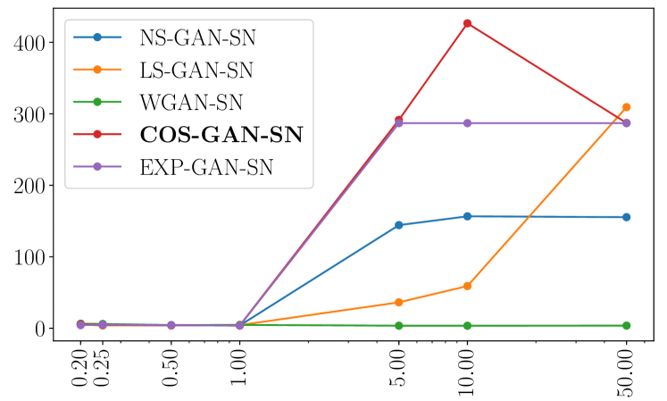
Refer to caption
(a) α=1e1𝛼1superscript𝑒1\alpha=1e^{1}, FID=6.55FID6.55\mathrm{FID}=6.55
Refer to caption
(b) α=1e3𝛼1superscript𝑒3\alpha=1e^{3}, FID=148.97FID148.97\mathrm{FID}=148.97
Refer to caption
(c) α=1e5𝛼1superscript𝑒5\alpha=1e^{5}, FID=134.44FID134.44\mathrm{FID}=134.44
Refer to caption
(d) α=1e7𝛼1superscript𝑒7\alpha=1e^{7}, FID=133.82FID133.82\mathrm{FID}=133.82
Refer to caption
(e) α=1e9𝛼1superscript𝑒9\alpha=1e^{9}, FID=130.21FID130.21\mathrm{FID}=130.21
Refer to caption
(f) α=1e11𝛼1superscript𝑒11\alpha=1e^{11}, FID=131.87FID131.87\mathrm{FID}=131.87
Refer to caption
Figure 36: Samples of randomly generated images with NS-GAN-SN of varying α𝛼\alpha (kSN=1.0subscript𝑘𝑆𝑁1.0k_{SN}=1.0, MNIST). For the line plot, x𝑥x-axis shows α𝛼\alpha (in log scale) and y𝑦y-axis shows the FID scores.
Refer to caption
(a) α=1e1𝛼1superscript𝑒1\alpha=1e^{1}, FID=23.37FID23.37\mathrm{FID}=23.37
Refer to caption
(b) α=1e3𝛼1superscript𝑒3\alpha=1e^{3}, FID=26.96FID26.96\mathrm{FID}=26.96
Refer to caption
(c) α=1e5𝛼1superscript𝑒5\alpha=1e^{5}, FID=260.05FID260.05\mathrm{FID}=260.05
Refer to caption
(d) α=1e7𝛼1superscript𝑒7\alpha=1e^{7}, FID=255.73FID255.73\mathrm{FID}=255.73
Refer to caption
(e) α=1e9𝛼1superscript𝑒9\alpha=1e^{9}, FID=256.96FID256.96\mathrm{FID}=256.96
Refer to caption
(f) α=1e11𝛼1superscript𝑒11\alpha=1e^{11}, FID=265.76FID265.76\mathrm{FID}=265.76
Refer to caption
Figure 37: Samples of randomly generated images with LS-GAN-SN of varying α𝛼\alpha (kSN=1.0subscript𝑘𝑆𝑁1.0k_{SN}=1.0, MNIST). For the line plot, x𝑥x-axis shows α𝛼\alpha (in log scale) and y𝑦y-axis shows the FID scores.
Refer to caption
(a) α=1e1𝛼1superscript𝑒1\alpha=1e^{1}, FID=13.43FID13.43\mathrm{FID}=13.43
Refer to caption
(b) α=1e3𝛼1superscript𝑒3\alpha=1e^{3}, FID=26.51FID26.51\mathrm{FID}=26.51
Refer to caption
(c) α=1e5𝛼1superscript𝑒5\alpha=1e^{5}, FID=271.85FID271.85\mathrm{FID}=271.85
Refer to caption
(d) α=1e7𝛼1superscript𝑒7\alpha=1e^{7}, FID=212.74FID212.74\mathrm{FID}=212.74
Refer to caption
(e) α=1e9𝛼1superscript𝑒9\alpha=1e^{9}, FID=274.63FID274.63\mathrm{FID}=274.63
Refer to caption
(f) α=1e11𝛼1superscript𝑒11\alpha=1e^{11}, FID=269.96FID269.96\mathrm{FID}=269.96
Refer to caption
Figure 38: Samples of randomly generated images with LS-GAN#-SN of varying α𝛼\alpha (kSN=1.0subscript𝑘𝑆𝑁1.0k_{SN}=1.0, MNIST). For the line plot, x𝑥x-axis shows α𝛼\alpha (in log scale) and y𝑦y-axis shows the FID scores.
Refer to caption
(a) α=1e1𝛼1superscript𝑒1\alpha=1e^{1}, FID=11.02FID11.02\mathrm{FID}=11.02
Refer to caption
(b) α=1e3𝛼1superscript𝑒3\alpha=1e^{3}, FID=286.96FID286.96\mathrm{FID}=286.96
Refer to caption
(c) α=1e5𝛼1superscript𝑒5\alpha=1e^{5}, FID=286.96FID286.96\mathrm{FID}=286.96
Refer to caption
(d) α=1e7𝛼1superscript𝑒7\alpha=1e^{7}, FID=286.96FID286.96\mathrm{FID}=286.96
Refer to caption
(e) α=1e9𝛼1superscript𝑒9\alpha=1e^{9}, FID=286.96FID286.96\mathrm{FID}=286.96
Refer to caption
(f) α=1e11𝛼1superscript𝑒11\alpha=1e^{11}, FID=286.96FID286.96\mathrm{FID}=286.96
Refer to caption
Figure 39: Samples of randomly generated images with EXP-GAN-SN of varying α𝛼\alpha (kSN=1.0subscript𝑘𝑆𝑁1.0k_{SN}=1.0, MNIST). For the line plot, x𝑥x-axis shows α𝛼\alpha (in log scale) and y𝑦y-axis shows the FID scores.
Refer to caption
(a) α=1e1𝛼1superscript𝑒1\alpha=1e^{1}, FID=11.79FID11.79\mathrm{FID}=11.79
Refer to caption
(b) α=1e3𝛼1superscript𝑒3\alpha=1e^{3}, FID=377.62FID377.62\mathrm{FID}=377.62
Refer to caption
(c) α=1e5𝛼1superscript𝑒5\alpha=1e^{5}, FID=375.72FID375.72\mathrm{FID}=375.72
Refer to caption
(d) α=1e7𝛼1superscript𝑒7\alpha=1e^{7}, FID=363.45FID363.45\mathrm{FID}=363.45
Refer to caption
(e) α=1e9𝛼1superscript𝑒9\alpha=1e^{9}, FID=401.12FID401.12\mathrm{FID}=401.12
Refer to caption
(f) α=1e11𝛼1superscript𝑒11\alpha=1e^{11}, FID=376.39FID376.39\mathrm{FID}=376.39
Refer to caption
Figure 40: Samples of randomly generated images with COS-GAN-SN of varying α𝛼\alpha (kSN=1.0subscript𝑘𝑆𝑁1.0k_{SN}=1.0, MNIST). For the line plot, x𝑥x-axis shows α𝛼\alpha (in log scale) and y𝑦y-axis shows the FID scores.
FID scores v.s. α𝛼\alpha (kSN=1.0subscript𝑘𝑆𝑁1.0k_{SN}=1.0) of Different Loss Functions
- CIFAR10 -
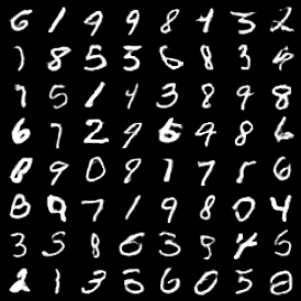
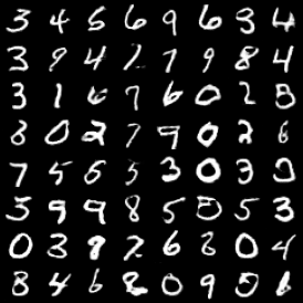
Refer to caption
(a) α=1e1𝛼1superscript𝑒1\alpha=1e^{1}, FID=17.63FID17.63\mathrm{FID}=17.63
Refer to caption
(b) α=1e3𝛼1superscript𝑒3\alpha=1e^{3}, FID=47.31FID47.31\mathrm{FID}=47.31
Refer to caption
(c) α=1e5𝛼1superscript𝑒5\alpha=1e^{5}, FID=46.85FID46.85\mathrm{FID}=46.85
Refer to caption
(d) α=1e7𝛼1superscript𝑒7\alpha=1e^{7}, FID=45.44FID45.44\mathrm{FID}=45.44
Refer to caption
(e) α=1e9𝛼1superscript𝑒9\alpha=1e^{9}, FID=45.67FID45.67\mathrm{FID}=45.67
Refer to caption
(f) α=1e11𝛼1superscript𝑒11\alpha=1e^{11}, FID=39.90FID39.90\mathrm{FID}=39.90
Refer to caption
Figure 41: Samples of randomly generated images with NS-GAN-SN of varying α𝛼\alpha (kSN=1.0subscript𝑘𝑆𝑁1.0k_{SN}=1.0, CIFAR10). For the line plot, x𝑥x-axis shows α𝛼\alpha (in log scale) and y𝑦y-axis shows the FID scores.
Refer to caption
(a) α=1e1𝛼1superscript𝑒1\alpha=1e^{1}, FID=25.55FID25.55\mathrm{FID}=25.55
Refer to caption
(b) α=1e3𝛼1superscript𝑒3\alpha=1e^{3}, FID=34.44FID34.44\mathrm{FID}=34.44
Refer to caption
(c) α=1e5𝛼1superscript𝑒5\alpha=1e^{5}, FID=373.07FID373.07\mathrm{FID}=373.07
Refer to caption
(d) α=1e7𝛼1superscript𝑒7\alpha=1e^{7}, FID=171.18FID171.18\mathrm{FID}=171.18
Refer to caption
(e) α=1e9𝛼1superscript𝑒9\alpha=1e^{9}, FID=309.55FID309.55\mathrm{FID}=309.55
Refer to caption
(f) α=1e11𝛼1superscript𝑒11\alpha=1e^{11}, FID=312.96FID312.96\mathrm{FID}=312.96
Refer to caption
Figure 42: Samples of randomly generated images with LS-GAN-SN of varying α𝛼\alpha (kSN=1.0subscript𝑘𝑆𝑁1.0k_{SN}=1.0, CIFAR10). For the line plot, x𝑥x-axis shows α𝛼\alpha (in log scale) and y𝑦y-axis shows the FID scores.
Refer to caption
(a) α=1e1𝛼1superscript𝑒1\alpha=1e^{1}, FID=20.45FID20.45\mathrm{FID}=20.45
Refer to caption
(b) α=1e3𝛼1superscript𝑒3\alpha=1e^{3}, FID=36.18FID36.18\mathrm{FID}=36.18
Refer to caption
(c) α=1e5𝛼1superscript𝑒5\alpha=1e^{5}, FID=429.21FID429.21\mathrm{FID}=429.21
Refer to caption
(d) α=1e7𝛼1superscript𝑒7\alpha=1e^{7}, FID=269.63FID269.63\mathrm{FID}=269.63
Refer to caption
(e) α=1e9𝛼1superscript𝑒9\alpha=1e^{9}, FID=291.55FID291.55\mathrm{FID}=291.55
Refer to caption
(f) α=1e11𝛼1superscript𝑒11\alpha=1e^{11}, FID=297.71FID297.71\mathrm{FID}=297.71
Refer to caption
Figure 43: Samples of randomly generated images with LS-GAN#-SN of varying α𝛼\alpha (kSN=1.0subscript𝑘𝑆𝑁1.0k_{SN}=1.0, CIFAR10). For the line plot, x𝑥x-axis shows α𝛼\alpha (in log scale) and y𝑦y-axis shows the FID scores.
Refer to caption
(a) α=1e1𝛼1superscript𝑒1\alpha=1e^{1}, FID=21.56FID21.56\mathrm{FID}=21.56
Refer to caption
(b) α=1e3𝛼1superscript𝑒3\alpha=1e^{3}, FID=401.24FID401.24\mathrm{FID}=401.24
Refer to caption
(c) α=1e5𝛼1superscript𝑒5\alpha=1e^{5}, FID=401.24FID401.24\mathrm{FID}=401.24
Refer to caption
(d) α=1e7𝛼1superscript𝑒7\alpha=1e^{7}, FID=401.24FID401.24\mathrm{FID}=401.24
Refer to caption
(e) α=1e9𝛼1superscript𝑒9\alpha=1e^{9}, FID=401.24FID401.24\mathrm{FID}=401.24
Refer to caption
(f) α=1e11𝛼1superscript𝑒11\alpha=1e^{11}, FID=401.24FID401.24\mathrm{FID}=401.24
Refer to caption
Figure 44: Samples of randomly generated images with EXP-GAN-SN of varying α𝛼\alpha (kSN=1.0subscript𝑘𝑆𝑁1.0k_{SN}=1.0, CIFAR10). For the line plot, x𝑥x-axis shows α𝛼\alpha (in log scale) and y𝑦y-axis shows the FID scores.
Refer to caption
(a) α=1e1𝛼1superscript𝑒1\alpha=1e^{1}, FID=18.59FID18.59\mathrm{FID}=18.59
Refer to caption
(b) α=1e3𝛼1superscript𝑒3\alpha=1e^{3}, FID=386.24FID386.24\mathrm{FID}=386.24
Refer to caption
(c) α=1e5𝛼1superscript𝑒5\alpha=1e^{5}, FID=259.83FID259.83\mathrm{FID}=259.83
Refer to caption
(d) α=1e7𝛼1superscript𝑒7\alpha=1e^{7}, FID=268.89FID268.89\mathrm{FID}=268.89
Refer to caption
(e) α=1e9𝛼1superscript𝑒9\alpha=1e^{9}, FID=293.29FID293.29\mathrm{FID}=293.29
Refer to caption
(f) α=1e11𝛼1superscript𝑒11\alpha=1e^{11}, FID=318.65FID318.65\mathrm{FID}=318.65
Refer to caption
Figure 45: Samples of randomly generated images with COS-GAN-SN of varying α𝛼\alpha (kSN=1.0subscript𝑘𝑆𝑁1.0k_{SN}=1.0, CIFAR10). For the line plot, x𝑥x-axis shows α𝛼\alpha (in log scale) and y𝑦y-axis shows the FID scores.
FID scores v.s. α𝛼\alpha (kSN=1.0subscript𝑘𝑆𝑁1.0k_{SN}=1.0) of Different Loss Functions
- CelebA -
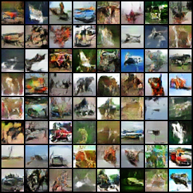
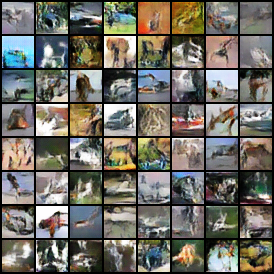
Refer to caption
(a) α=1e1𝛼1superscript𝑒1\alpha=1e^{1}, FID=5.88FID5.88\mathrm{FID}=5.88
Refer to caption
(b) α=1e3𝛼1superscript𝑒3\alpha=1e^{3}, FID=16.14FID16.14\mathrm{FID}=16.14
Refer to caption
(c) α=1e5𝛼1superscript𝑒5\alpha=1e^{5}, FID=17.75FID17.75\mathrm{FID}=17.75
Refer to caption
(d) α=1e7𝛼1superscript𝑒7\alpha=1e^{7}, FID=17.67FID17.67\mathrm{FID}=17.67
Refer to caption
(e) α=1e9𝛼1superscript𝑒9\alpha=1e^{9}, FID=16.87FID16.87\mathrm{FID}=16.87
Refer to caption
(f) α=1e11𝛼1superscript𝑒11\alpha=1e^{11}, FID=18.81FID18.81\mathrm{FID}=18.81
Refer to caption
Figure 46: Samples of randomly generated images with NS-GAN-SN of varying α𝛼\alpha (kSN=1.0subscript𝑘𝑆𝑁1.0k_{SN}=1.0, CelebA). For the line plot, x𝑥x-axis shows α𝛼\alpha (in log scale) and y𝑦y-axis shows the FID scores.
Refer to caption
(a) α=1e1𝛼1superscript𝑒1\alpha=1e^{1}, FID=8.41FID8.41\mathrm{FID}=8.41
Refer to caption
(b) α=1e3𝛼1superscript𝑒3\alpha=1e^{3}, FID=12.09FID12.09\mathrm{FID}=12.09
Refer to caption
(c) α=1e5𝛼1superscript𝑒5\alpha=1e^{5}, FID=201.22FID201.22\mathrm{FID}=201.22
Refer to caption
(d) α=1e7𝛼1superscript𝑒7\alpha=1e^{7}, FID=312.83FID312.83\mathrm{FID}=312.83
Refer to caption
(e) α=1e9𝛼1superscript𝑒9\alpha=1e^{9}, FID=299.30FID299.30\mathrm{FID}=299.30
Refer to caption
(f) α=1e11𝛼1superscript𝑒11\alpha=1e^{11}, FID=321.84FID321.84\mathrm{FID}=321.84
Refer to caption
Figure 47: Samples of randomly generated images with LS-GAN-SN of varying α𝛼\alpha (kSN=1.0subscript𝑘𝑆𝑁1.0k_{SN}=1.0, CelebA). For the line plot, x𝑥x-axis shows α𝛼\alpha (in log scale) and y𝑦y-axis shows the FID scores.
Refer to caption
(a) α=1e1𝛼1superscript𝑒1\alpha=1e^{1}, FID=7.21FID7.21\mathrm{FID}=7.21
Refer to caption
(b) α=1e3𝛼1superscript𝑒3\alpha=1e^{3}, FID=13.13FID13.13\mathrm{FID}=13.13
Refer to caption
(c) α=1e5𝛼1superscript𝑒5\alpha=1e^{5}, FID=221.41FID221.41\mathrm{FID}=221.41
Refer to caption
(d) α=1e7𝛼1superscript𝑒7\alpha=1e^{7}, FID=248.48FID248.48\mathrm{FID}=248.48
Refer to caption
(e) α=1e9𝛼1superscript𝑒9\alpha=1e^{9}, FID=311.21FID311.21\mathrm{FID}=311.21
Refer to caption
(f) α=1e11𝛼1superscript𝑒11\alpha=1e^{11}, FID=315.94FID315.94\mathrm{FID}=315.94
Refer to caption
Figure 48: Samples of randomly generated images with LS-GAN#-SN of varying α𝛼\alpha (kSN=1.0subscript𝑘𝑆𝑁1.0k_{SN}=1.0, CelebA). For the line plot, x𝑥x-axis shows α𝛼\alpha (in log scale) and y𝑦y-axis shows the FID scores.
Refer to caption
(a) α=1e1𝛼1superscript𝑒1\alpha=1e^{1}, FID=6.91FID6.91\mathrm{FID}=6.91
Refer to caption
(b) α=1e3𝛼1superscript𝑒3\alpha=1e^{3}, FID=375.32FID375.32\mathrm{FID}=375.32
Refer to caption
(c) α=1e5𝛼1superscript𝑒5\alpha=1e^{5}, FID=375.32FID375.32\mathrm{FID}=375.32
Refer to caption
(d) α=1e7𝛼1superscript𝑒7\alpha=1e^{7}, FID=375.32FID375.32\mathrm{FID}=375.32
Refer to caption
(e) α=1e9𝛼1superscript𝑒9\alpha=1e^{9}, FID=375.32FID375.32\mathrm{FID}=375.32
Refer to caption
(f) α=1e11𝛼1superscript𝑒11\alpha=1e^{11}, FID=375.32FID375.32\mathrm{FID}=375.32
Refer to caption
Figure 49: Samples of randomly generated images with EXP-GAN-SN of varying α𝛼\alpha (kSN=1.0subscript𝑘𝑆𝑁1.0k_{SN}=1.0, CelebA). For the line plot, x𝑥x-axis shows α𝛼\alpha (in log scale) and y𝑦y-axis shows the FID scores.
Refer to caption
(a) α=1e1𝛼1superscript𝑒1\alpha=1e^{1}, FID=6.62FID6.62\mathrm{FID}=6.62
Refer to caption
(b) α=1e3𝛼1superscript𝑒3\alpha=1e^{3}, FID=450.57FID450.57\mathrm{FID}=450.57
Refer to caption
(c) α=1e5𝛼1superscript𝑒5\alpha=1e^{5}, FID=233.42FID233.42\mathrm{FID}=233.42
Refer to caption
(d) α=1e7𝛼1superscript𝑒7\alpha=1e^{7}, FID=390.40FID390.40\mathrm{FID}=390.40
Refer to caption
(e) α=1e9𝛼1superscript𝑒9\alpha=1e^{9}, FID=306.17FID306.17\mathrm{FID}=306.17
Refer to caption
(f) α=1e11𝛼1superscript𝑒11\alpha=1e^{11}, FID=335.87FID335.87\mathrm{FID}=335.87
Refer to caption
Figure 50: Samples of randomly generated images with COS-GAN-SN of varying α𝛼\alpha (kSN=1.0subscript𝑘𝑆𝑁1.0k_{SN}=1.0, CelebA). For the line plot, x𝑥x-axis shows α𝛼\alpha (in log scale) and y𝑦y-axis shows the FID scores.
FID scores of WGAN-SN and some extremely degenerate loss functions (α=1e25𝛼1superscript𝑒25\alpha=1e^{-25})
on different datasets
Refer to caption
(a) WGAN, FID=3.71FID3.71\mathrm{FID}=3.71
Refer to caption
(b) WGAN, FID=23.36FID23.36\mathrm{FID}=23.36
Refer to caption
(c) WGAN, FID=7.82FID7.82\mathrm{FID}=7.82
Refer to caption
(d) NSGAN, FID=3.74FID3.74\mathrm{FID}=3.74
Refer to caption
(e) NSGAN, FID=21.92FID21.92\mathrm{FID}=21.92
Refer to caption
(f) NSGAN, FID=8.10FID8.10\mathrm{FID}=8.10
Refer to caption
(g) LSGAN#, FID=3.81FID3.81\mathrm{FID}=3.81
Refer to caption
(h) LSGAN#, FID=21.47FID21.47\mathrm{FID}=21.47
Refer to caption
(i) LSGAN#, FID=8.51FID8.51\mathrm{FID}=8.51
Refer to caption
(j) COSGAN, FID=3.96FID3.96\mathrm{FID}=3.96
Refer to caption
(k) COSGAN, FID=23.65FID23.65\mathrm{FID}=23.65
Refer to caption
(l) COSGAN, FID=8.30FID8.30\mathrm{FID}=8.30
Refer to caption
(m) EXPGAN, FID=3.86FID3.86\mathrm{FID}=3.86
Refer to caption
(n) EXPGAN, FID=21.91FID21.91\mathrm{FID}=21.91
Refer to caption
(o) EXPGAN, FID=8.22FID8.22\mathrm{FID}=8.22
Figure 51: Samples of randomly generated images with WGAN-SN and some extremely degenerate loss functions (α=1e25𝛼1superscript𝑒25\alpha=1e^{-25}) on different datasets. We use kSN=50subscript𝑘𝑆𝑁50k_{SN}=50 for all our experiments.