Random diffusivity from stochastic equations: comparison of two models for Brownian yet non-Gaussian diffusion

Abstract

A considerable number of systems have recently been reported in which Brownian yet non-Gaussian dynamics was observed. These are processes characterised by a linear growth in time of the mean squared displacement, yet the probability density function of the particle displacement is distinctly non-Gaussian, and often of exponential (Laplace) shape. This apparently ubiquitous behaviour observed in very different physical systems has been interpreted as resulting from diffusion in inhomogeneous environments and mathematically represented through a variable, stochastic diffusion coefficient. Indeed different models describing a fluctuating diffusivity have been studied. Here we present a new view of the stochastic basis describing time dependent random diffusivities within a broad spectrum of distributions. Concretely, our study is based on the very generic class of the generalised Gamma distribution. Two models for the particle spreading in such random diffusivity settings are studied. The first belongs to the class of generalised grey Brownian motion while the second follows from the idea of diffusing diffusivities. The two processes exhibit significant characteristics which reproduce experimental results from different biological and physical systems. We promote these two physical models for the description of stochastic particle motion in complex environments.

1 Introduction

The systematic study of the diffusive motion of tracer particles in fluids dates back to the 19th century, particularly referring to Robert Brown’s experiments observing the erratic motion of granules extracted from pollen grains which were suspended in water [1]. Since then numerous scientists contributed by improving the experiments [2, 3, 4] as well as in defining the basis of the theory of diffusion [5, 6, 7, 8, 9]. In brief, Brownian or standard diffusion processes are mainly characterised by two central features: (i) the linear growth in time of the mean-squared displacement (MSD),

$$\langle x^{2}(t)\rangle=2Dt,$$ (1)

where $D$ is the diffusion coefficient, and (ii) the Gaussian probability density function (PDF) for the particle displacement,

$$G(x,t|D)=\frac{1}{\sqrt{4\pi Dt}}\exp\left(-\frac{x^{2}}{4Dt}\right).$$ (2)

Here and in the following we focus on a one-dimensional formulation of the model, a generalisation to higher dimensions can be achieved component-wise.

Discoveries of deviations from the linear time dependence (1) have a long history. Thus, Richardson already in 1926 reported his famed $t$-cubed law for the relative particle diffusion in turbulence [10]. Scher and Montroll uncovered anomalous diffusion of the power-law form

$$\langle x^{2}(t)\rangle\simeq D_{\alpha}t^{\alpha},$$ (3)

with the anomalous diffusion exponent $0<\alpha<1$ and the generalised diffusion coefficient $D_{\alpha}$ [11], for the motion of charge carriers in amorphous semiconductors [12]. With the advance of modern microscopy techniques, in particular, superresolution microscopy, as well as massive progress in supercomputing, anomalous diffusion of the type (3) has been reported in numerous complex and biological systems [13, 14]. Thus, subdiffusion with $0<\alpha<1$ was observed for submicron tracers in the crowded cytoplasm of biological cells [15, 16, 17, 18, 19] as well as in artificially crowded environments [20, 21, 22, 23]. Further reports of subdiffusion come from the motion of proteins embedded in the membranes of living cells [24, 25, 26]. Subdiffusion is also seen in extensive simulations studies, for instance, of lipid bilayer membranes [27, 28, 29, 30] and relative diffusion in proteins [31]. Superdiffusion, due to active motion of molecular motors, was observed in various biological cell types for both introduced and endogenous tracers [16, 17, 32, 33].

Most of the anomalous diffusion phenomena mentioned here belong to two main classes of anomalous diffusion: (i) the class of continuous time random walk processes, in which scale-free power-law waiting times in between motion events give rise to the law (3) [12, 34], along with a stretched Gaussian displacement probability density $G(x,t)$ [11, 12, 34] as well as weak ergodicity breaking and ageing [35, 36]. We note that similar effects of non-Gaussianity, weak non-ergodicity, and ageing also occur in spatially heterogeneous diffusion processes [37, 38, 39, 40]. (ii) The second one is the class of viscoelastic diffusion described by the generalised Langevin equation with power-law friction kernel [41, 42] and of fractional Brownian motion [43]. These processes are both fuelled by long-range, power-law correlated noise. Its distribution is Gaussian, so that the displacement probability density $G(x,t)$ is Gaussian, as well. Moreover, these are ergodic processes [23, 42, 44, 45, 46].

Over the last few years a new class of diffusive processes has been reported, namely, so-called Brownian yet non-Gaussian diffusion [47, 48]. This class identifies a dynamics characterised by a linear growth (1) of the MSD combined with a non-Gaussian probability density function for the particle displacement. The emergence of a non-Gaussian distribution, despite the Brownian MSD scaling, suggests the presence of an inhomogeneity that can be located both on the single tracer particle and on the ensemble levels. The study of these processes is becoming increasingly relevant with the growing number of complex systems discovered to exhibit such statistical features. For instance, we mention soft matter and biological systems, in which the motion of biological macromolecules, proteins and viruses along lipid tubes and through actin networks [47, 48], as well as along membranes and inside colloidal suspension [49] and colloidal nanoparticles adsorbed at fluid interfaces [50, 51, 52] are studied. We also mention ecological processes, involving the characterisation of organism movement and dispersal [53, 54], as well as processes, that are Brownian but non-Gaussian in certain time windows of their dynamics. These concern the dynamics of disordered solids, such as glasses and supercooled liquids [55, 56, 57] as well as interfacial dynamics [58, 59]. Also anomalous diffusion processes of the viscoelastic class that typically are expected to exhibit Gaussian statistic of displacements, were reported to have non-Gaussian displacements along with distinct distributions of diffusivity values. These concern the motion of tracer particles in the cellular cytoplasm [60, 61, 62] and the motion of lipids and proteins in protein-crowded model membranes [29].

Here we study two alternative stochastic approaches to non-Gaussian diffusion due to random diffusivity parameters, namely, generalised grey Brownian motion (ggBM) and diffusing diffusivities (DD). We analyse their exact behaviour and relate these approaches to the idea of superstatistics. To prepare the discussion, section 2 presents a primer on the approach of superstatistics and what has been done in the context of ggBM and DD models. In section 3 we then study the ggBM model with a random diffusivity distributed according to the generalised Gamma distribution. In particular, ggBM will be shown to represent a stochastic description of the superstatistics approach and is equivalent to the short time limit of the DD model. In section 4 we formulate a set of stochastic equations for the dynamics within the DD framework, in which the diffusivity statistic is governed by the generalised Gamma distribution. This is then incorporated in the framework of the minimal model of DD in section 5. In section 5.4 we describe the behaviour of the kurtosis of the two models, an important quantity for data analysis. Section 6 introduces an analysis for an initial non-equilibrium setting for the random diffusivity, relevant, for instance, for the description of single particle trajectories. To transfer this concept to the ggBM approach we propose a non-equilibrium version of ggBM. Finally our conclusions are reported in section 7. In the Appendices some mathematical details are collected.

2 Pathways to Brownian yet non-Gaussian diffusion: superstatistics and diffusing diffusivity, and generalised grey Brownian motion

When we talk about an ensemble of particles, we could imagine that non-Gaussian statistic in this ensemble sense emerges due to the fact that different particles are located in different environments with different transport characteristics, such as the diffusion coefficient. If during the observation time each particle remains in its own environment characterised by a given value $D$ of the diffusivity, the ensemble of particles shows a mixture of individual Gaussians, weighted by some distribution $p(D)$ of local diffusivities. This is the idea behind superstatistics, an approach promoted by Beck and Cohen [63], see also [64]. As a result, the ensemble dynamics is still Brownian yet the PDF of particle displacements will correspond to a sum or integral of single Gaussians with specific value of $D$, weighted by the distribution $p(D)$. For instance, an exponential form for $p(D)$ will produce an exponential shape of the ensemble displacement PDF, sometimes called a Laplace distribution. We note that there also exist superstatistical formulations on the basis of the stochastic Langevin equation, leading to Brownian yet non-Gaussian behaviour [65]. A quite general superstatistical formulation in terms of the gamma distribution was put forward by Hapca et al. [53].

More recently, similar concepts have been sought to describe non-Gaussian viscoelastic subdiffusion. Thus, Lampo et al. [61] observed exponential distributions of the generalised diffusivity $D_{\alpha}$ for the motion of submicron tracers in living bacteria and eukaryotic cells. As a theoretical description they used a superstatistical formulation of the stochastic equation for fractional Brownian motion [61]. Following the observation of stretched Gaussian shapes of the displacement PDF in protein-crowded lipid bilayer membranes [29], more general forms for the distribution of the generalised diffusion coefficient were introduced, see, for instance, [66, 67]. Viscoelastic, non-Gaussian diffusion was also described in terms of the generalised Langevin equation with superstatistical distribution of the friction amplitude [68, 69].

Some other models instead introduce a fluctuating diffusivity, for instance to describe segregation in solids [70] or to analyse data from diffusion processes assessed by modern measurement techniques [71]. Brownian motion in fluctuating environments, or governed by temperature or friction fluctuations has been studied in [72, 73, 74] and models with intermittency between two values of the diffusivity are considered in [75, 76]. Anomalous diffusion in a disordered system was also described in terms of a superstatistical model based on a Langevin equation formulation, combining a Rayleigh-shaped diffusivity distribution with deterministic power-law growth or decay of the mean diffusivity [77].

A general framework for the description of diffusion in complex environment is provided also by the class of stochastic processes identified as generalised grey Brownian motion (ggBM) [78, 79, 80, 81, 82]. The basic idea of this approach is that the complexity or heterogeneity of the medium is completely described by the random nature of a specific parameter. Choosing this parameter to be the diffusivity leads to a stochastic interpretation of the system that may be viewed as complementary to the superstatistics concept and thus suitable for the description of the class of Brownian yet non-Gaussian processes. We will define ggBM with a random diffusivity in more detail in the next section 3, and in the following demonstrate that ggBM is equivalent to th short time limit of the DD model.

Recently the idea of DD has received considerable attention. According to this approach, in addition to the introduction of a population of diffusivities, each particle during its motion is affected by a continuously changing diffusivity. Chubynsky and Slater first introduced this model describing the dynamics of the diffusion coefficient by a biased, stationary random walk with reflecting boundary conditions [83]. With this assumption the diffusivity changes slowly step by step, in the short time limit giving rise to normal diffusion with exponential displacement PDF. In the long time regime simulations showed a crossover to Gaussian diffusion with a single, effective diffusion coefficient [83]. In a more recent work a direct test of the DD mechanism for diffusion in inhomogeneous media is reported [86].

The DD concept was further studied by Jain and Sebastian [87, 88] and Chechkin et al[67]. While Jain and Sebastian use a path integral approach, Chechkin et alinvoke the concept of subordination and an explicit exact solution for the PDF in Fourier space. Despite the different mathematical approach, both models recover the linear trend of the MSD and a distribution of displacements that at short times is exponential, while, at long times, it crosses over to a Gaussian with effective diffusivity, in agreement with the results in [83]. Tyagi and Cherayil [89] present a hybrid procedure between the two approaches, finding that the modulation of white noise by any stochastic process, whose time correlation function decays exponentially, is likely to have features similar to the ones obtained in [67, 83, 87, 88]. As a recent result we also report the work by Lanoiselée and Grebenkov in which the concept of DD is further investigated, for instance, with respect to time averages and ergodicity breaking properties [90].

In this paper we present a detailed comparison between the concept of ggBM with random diffusivity and the DD model. The main difference between the DD and ggBM model is represented by the interaction between environment and particles. On the one hand, in the DD model two different statistical levels are taken into account, one for the motion of the environment and one for the motion of the particles. The relation between these two gives rise to specific characteristics. Thus, at short times the slow variability of the environment guarantees the superstatistical limit. In the long time regime the diffusivity reaches a stationary average value leading the particles to develop a Gaussian statistic. On the other hand, the ggBM model does not directly involve an environment dynamics but only implies a dynamics in which the statistical features of the environment continuously drives the particles in their motion, see below for more details.

Concretely, for both ggBM and DD models a set of stochastic equations is introduced to generate a time dependent random diffusivity with a well defined stationary distribution. Until now mainly exponential or Gamma distributions have been considered for the random diffusivity. We here base the discussion on the generalised Gamma distribution, which represents an even broader class of distributions including the ones mentioned above, as particular cases. We define the generalised Gamma distribution by

$$\gamma^{\mathrm{gen}}_{\nu,\eta}(D)=\frac{\eta}{D_{\star}^{\nu}\,\Gamma(\nu/\eta)}D^{\nu-1}\exp\left(-\left[\frac{D}{D_{\star}}\right]^{\eta}\right),$$ (4)

where $D_{\star}$ is a positive and dimensional constant and $\nu$ and $\eta$ are positive constants. This distribution encodes the $n$th order stationary moments

$$\langle D^{n}\rangle_{\mathrm{stat}}=D_{\star}^{n}\frac{\Gamma([\nu+n]/\eta)}{\Gamma(\nu/\eta)}.$$ (5)

The choice of the generalised Gamma distribution is based on experimental evidence demonstrating its role as a versatile description for generalised distributions in various complex systems. Indeed, in the context of superstatistics the generalised Gamma distribution was studied by Beck in [91]. Importantly, the generalised Gamma distribution includes those cases labelled as Gamma or exponential distribution that have already shown good agreement with several systems [53, 55, 56, 57]. Moreover it comprises the cases of stretched and compressed exponential distributions which may be useful for the interpretation of various systems [26, 53, 92, 93].

In the following we generalise the ggBM model from references [78, 79, 80, 81, 82] to incorporate the generalised Gamma function (4). We then demonstrate how to reformulate the Ornstein-Uhlenbeck picture of the DD minimal model [67] and the closely related DD models [83, 87, 88] to include the distribution (4). With this extension both models are considerably more flexible for the description of measured data. Moreover, we will show that the ggBM model is a powerful stochastic representation of the superstatistics approach, and that the ggBM model equals the short time limit of the DD model. Finally, we consider non-equilibrium conditions in the DD model and propose a non-equilibrium extension of the ggBM model to consider similar effects in the stochastic setting of superstatistics. Such non-equilibrium initial conditions represent an important extension of the random diffusivity models, especially for experimentally relevant cases of single particle trajectory measurements.

3 Generalised grey Brownian motion with random diffusivity

GgBM is defined through the stochastic equation [78, 79, 80, 81, 82]

$$X_{\mathrm{ggBM}}(t)=\sqrt{2D}\times W(t),$$ (6)

for the particle trajectory $X_{\mathrm{ggBM}}(t)$, in which $W(t)=\int_{0}^{t}\xi(t^{\prime})dt^{\prime}$ is standard Brownian motion, the Wiener process defined as the integral over the white Gaussian noise $\xi(t)$ with zero mean. Moreover, $D$ is a random diffusivity, here taken to be distributed according to the generalised Gamma distribution (4). The idea is that different, but physically identical particles move in disjointed environments, in which they experience different diffusivities, the essential view of the superstatistics approach. Alternatively, we could also think of physically different particles, with different diffusion coefficients, moving in an identical environment. The latter could, for instance, correspond to an ensemble of tracer beads with varying radius or different surface properties.

More mathematically speaking, ggBM is defined through the explicit construction of the underlying probability space based on self-similar increments, and it can be represented by the stochastic equation $X_{\mathrm{ggBM}}=\sqrt{\Lambda}X_{g}$, where $\Lambda$ is an independent, non-negative random variable, and $X_{g}$ is a Gaussian process [78, 79, 80, 81, 82]. The characterisation of this class has also been studied for the case when $X_{g}$ is a standard fractional Brownian motion (FBM) and $\Lambda$ is distributed according to the quite general class of M-Wright functions [81, 94]. We note that the definition (6) is similar to the superstatistical Langevin equation models in [65, 77].

Figure 1: Top: Trajectories governed by the ggBM model for $\eta=1.3$ and two different parameters $\nu$ (see figure legend). Bottom: Time averaged MSD for the respective traces shown in the top panel, with identical colour coding. The different trajectories exhibit random diffusivity values and thus random slopes in the time averaged MSD plots. Within each trajectory the value of $D$ remains fixed.

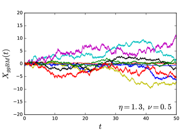
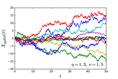
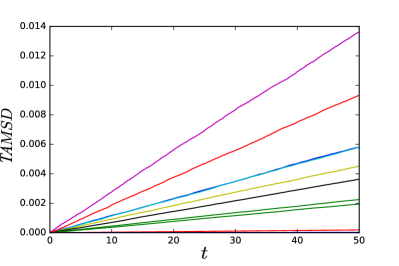
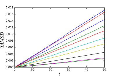
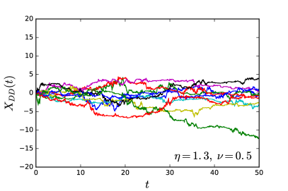
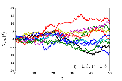
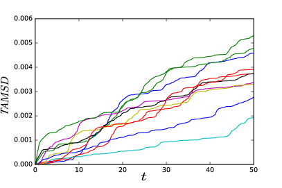
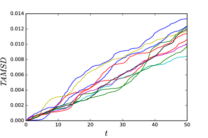
Figure 1 shows trajectories obtained from direct simulations of the scheme (6), for which the diffusivity values $D$ are chosen from the generalised Gamma distribution (4). As a result we obtain a Brownian motion characterised by a random amplitude, as demonstrated explicitly by the MSD plots for the same trajectories shown in the bottom panel of figure 1. For the value $\nu=1.5$ (right panels) larger $D$ values are observed, in accordance with the shape of the distribution (4). The ggBM description is indeed close to the superstatistical concept and fundamentally different from the time evolution of the sample paths for the DD model, compare figure 7. However, at very short times both processes look much alike, as the DD model at short times will be shown to reduce to the ggBM model.

The particle displacement distribution can be recovered following Pagnini and Paradisi [94]. If we define with $Z_{1}$ and $Z_{2}$ two real independent random variables whose PDFs are $p_{1}(z_{1})$ and $p_{2}(z_{2})$ with $-\infty\leq z_{1}\leq+\infty$ and $0\leq z_{2}\leq+\infty$, respectively, and with the random variable $Z$ obtained by the product of $Z_{1}$ and $Z_{2}^{\gamma}$, that is, $Z=Z_{1}Z_{2}^{\gamma}$, then, if we denote the PDF of $Z$ with $p(z)$, we find that

$$p(z)=\int_{0}^{\infty}p_{1}\left(\frac{z}{\lambda^{\gamma}}\right)p_{2}(\lambda)\frac{d\lambda}{\lambda^{\gamma}}.$$ (7)

In the present case we identify $X_{ggBM}(t)$, $W(t)$, and the random diffusivity $D$ with $Z$, $Z_{1}$, and $Z_{2}$, respectively. The PDF for the particle displacement encoded by equation (6) and (7) is given by

$$f_{\mathrm{ggBM}}(x,t) = \int_{0}^{\infty}\frac{1}{\sqrt{2\pi t}}\exp\left(-\frac{\left(x/\sqrt{2D}\right)^{2}}{2t}\right)p_{D}(D)\frac{dD}{\sqrt{2D}}$$ (8)

$$= \int_{0}^{\infty}\frac{1}{\sqrt{4\pi Dt}}\exp\left(-\frac{x^{2}}{4Dt}\right)p_{D}(D)dD$$

$$= \int_{0}^{\infty}G(x,t|D)p_{D}(D)dD,$$

where $G(x,t|D)$ is the Gaussian distribution (2) for given $D$. Such a representation of the PDF corresponds to the one of the superstatistical approach, proving the similarity of the two methods. The distribution $p_{D}(D)$ is defined in (4) and the integral in (8), which can be solved exactly through different methods (Appendix A.1), provides the result (12adbv) in terms of a Fox $H$-function (see Appendix A.1, where also the series expansion is given). The asymptotic behaviour of this result acquires the generalised exponential shape

$$f_{\mathrm{ggBM}}(x,t)\sim\frac{(x^{2}/[4D_{\star}t])^{(2\nu-\eta-1)/(2[\eta+1])}}{\Gamma(\nu/\eta)\sqrt{4\pi D_{\star}t}}\exp\left(-\frac{\eta+1}{\eta}\eta^{\frac{1}{\eta+1}}\left[\frac{x^{2}}{4D_{\star}t}\right]^{\eta/(\eta+1)}\right).$$ (9)

In particular, the choice $\eta=1$ leads us back to exponential distributions, with power-law prefactor. Figure 2 demonstrates the agreement between the analytical result (9) for the PDF and the result of stochastic simulations of the underlying ggBM process, for different times and a fixed set of the parameters $\nu$ and $\eta$. In particular, we see that the shape of the distribution remains invariant—as for the superstatistical approach—and in contrast to the DD model analysed below.

Figure 2: Short (a) and long (b) time behaviour of the PDF of the ggBM process for the parameters $\eta=1.3$ and $\nu=0.5$, as well as $D_{\star}=1/2$. Solid lines represent the asymptotic behaviour (9), while symbols are obtained from stochastic simulations of the ggBM process.

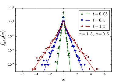
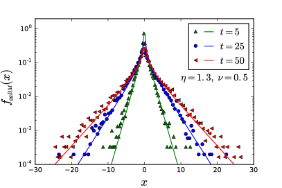
The MSD follows immediately from the following transformations,

$$\langle X_{\mathrm{ggBM}}^{2}(t)\rangle = \int_{-\infty}^{\infty}x^{2}f_{\mathrm{ggBM}}(x,t)dx$$ (10)

$$= \int_{0}^{\infty}p_{D}(D)\int_{-\infty}^{\infty}x^{2}G(x,t|D)dxdD$$

$$= \int_{0}^{\infty}p_{D}(D)2DtdD=2t\int_{0}^{\infty}Dp_{D}(D)dD$$

$$= 2\langle D\rangle_{\mathrm{stat}}t,$$

where, according to (5), the effective diffusivity becomes

$$\langle D\rangle_{\mathrm{stat}}=D_{\star}\Gamma([\nu+1]/\eta)/\Gamma(\nu/\eta).$$ (11)

Figure 3 demonstrates the linearity of the variance. The fitted parameters are consistent with the model prediction, $\langle D\rangle_{\mathrm{stat}}=0.20$ comparing to the values chosen in the simulations.

Figure 3: Variance of the ggBM model (blue line) and linear fit (solid line). The corresponding fit parameters are indicated in the figure legend. The value of $D_{\star}=1/2$.

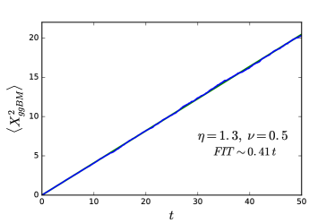
By means of the ggBM approach and with the introduction of a generalised Gamma distribution for the diffusivity we are able to reproduce a diffusive motion with a linear scaling of the MSD and a PDF characterised by a stretched or compressed Gaussian with a power-law prefactor. This is our first main result.

4 Diffusing diffusivity: stochastic equations for random diffusivity

We now consider the diffusion coefficient $D(t)$ to be a random function of time, defined by means of the auxiliary variable $Y(t)$ through $D(t)=Y^{2}(t)$, similarly to the DD minimal model introduced earlier [67]. Our goal is to construct a stochastic equation for the additional variable $Y(t)$ such that the stationary PDF for its square is the generalised Gamma distribution in (4). Thus, our present model is represented by the following set of stochastic equations

$$dY = a(Y)dt+\sigma\times dW(t)$$ (12a)

$$D(t) = Y^{2}(t),$$ (12b)

where $a(Y)$ is a nonlinear function whose explicit shape is obtained below, $\sigma$ is a constant and $W(t)$ is a Wiener process with variance $\langle W^{{}^{2}}(t)\rangle=t$. The physical dimension of the auxiliary variable is $[Y]=\mathrm{cm}/\mathrm{sec}^{1/2}$ and for the constant $\sigma$ we have $[\sigma]=\mathrm{cm}/\mathrm{sec}$.

Our approach is based on the central idea that it is possible to establish a direct relation between the PDFs of the two variables $Y(t)$ and $D(t)$. This allows us to introduce a completely new dynamics for the auxiliary variable. Such a dynamics, even though more complex, allows to reproduce a more general class of PDFs for the random diffusivity and thus provides a significant extension of the DD model, which will be our second main result.

To proceed we set $p(Y,t)$ to represent the PDF of the process $Y(t)$ described in (12a). It fulfils the Fokker-Plank equation [9]

$$\frac{\partial p(Y,t)}{\partial t}+\frac{\partial a(Y)p(Y,t)}{\partial Y}=\frac{\sigma^{2}}{2}\frac{\partial^{2}p(Y,t)}{\partial Y^{2}}.$$ (12m)

Considering the stationary situation the corresponding time independent PDF $p_{Y}(Y)$ fulfils the equation

$$\frac{\partial a(Y)p_{Y}(Y)}{\partial Y}=\frac{\sigma^{2}}{2}\frac{\partial^{2}p_{Y}(Y)}{\partial Y^{2}},$$ (12n)

from which we infer the relation

$$a(Y)=\frac{\sigma^{2}}{2p_{Y}(Y)}\frac{\partial p_{Y}(Y)}{\partial Y},$$ (12o)

directly relating the drift coefficient $a(Y)$ with the stationary distribution of $Y(t)$ [95].

We then recall that, given two random variables $Z_{1}$ and $Z_{2}$ related by $Z_{2}=g(Z_{1})$, for appropriate functions $g(z)$ we have [96]

$$p_{Z_{2}}(z_{2})=p_{Z_{1}}\big{(}g^{-1}(z_{2})\big{)}\left|\frac{d}{dz_{2}}g^{-1}(z_{2})\right|.$$ (12p)

This implies that the distributions of the variables $Y(t)$ and $D(t)$ are related via

$$p_{Y}(Y,t)=|Y|p_{D}(Y^{2},t).$$ (12q)

Based on this we construct a set of stochastic equations for the desired quantity $D(t)$. Starting from the chosen stationary distribution $p_{D}(D)$ of the random diffusivity we define the stationary distribution $p_{Y}(Y)$ for the auxiliary variable $Y(t)$ by means of equation (12q). Finally relation (12o) allows us to recover the suitable coefficient $a(Y)$ in equation (12a). Following the described scheme for the generalised Gamma distribution (4) we obtain

$$p_{Y}(Y)=|Y|\frac{\eta}{D_{\star}^{\nu}\Gamma(\nu/\eta)}Y^{2(\nu-1)}\exp\left(-\left[\frac{Y}{\sqrt{D_{\star}}}\right]^{2\eta}\right),$$ (12r)

and thus

$$\frac{\partial p_{Y}(Y)}{\partial Y}(Y)=\frac{\eta\mathrm{sgn}(Y)}{D_{\star}^{\nu}\Gamma(\nu/\eta)}Y^{2(\nu-1)}\exp\left(-\left[\frac{Y}{\sqrt{D_{\star}}}\right]^{2\eta}\right)\left(2\nu-1-2\eta\left[\frac{Y}{\sqrt{D_{\star}}}\right]^{2\eta}\right).$$ (12s)

This finally leads us to the desired drift coefficient

$$a(Y)=\frac{\sigma^{2}}{2Y}\left(2\nu-1-2\eta\left[\frac{Y}{\sqrt{D_{\star}}}\right]^{2\eta}\right).$$ (12t)

The stochastic equations (12a) together with the explicit form (12t) of the drift coefficient for the diffusivity fluctuations provide a complete and generalised analogue of the DD model, which is extremely flexible for the modelling of experimental data.

We notice that in the particular case of $\nu=0.5$ and $\eta=1$ we recover the Ornstein-Uhlenbeck model (diffusion in an harmonic potential) considered in the original minimal DD model [67]. As already remarked in [67] in this setting the resulting stochastic equation for $D(t)$ is nothing else than the Heston model, that is widely used in financial mathematics and specifies the time evolution of the stochastic volatility of a given asset [90, 97, 98].

Figure 4: Top: Trajectories and bottom: autocorrelation functions (12u), of the auxiliary variable $Y(t)$ and the random diffusivity $D(t)$ in the DD model. The green solid lines in the autocorrelation function plots represent exponential fits. We took $\nu=0.5$ and $\eta=1.3$.

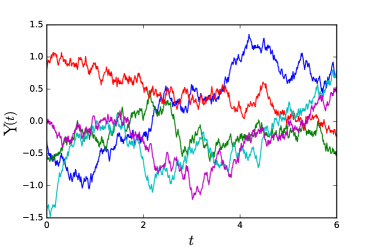
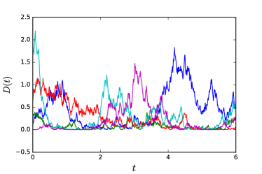
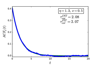
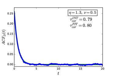
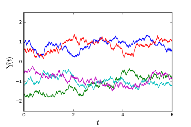
Equation (12a) can be readily solved numerically with initial conditions taken randomly from the equilibrium distribution (12r). Figures 4 and 5 show sample time evolutions of the auxiliary variable $Y$ and the diffusivity $D=Y^{2}$ for the DD process based on the steady state generalised Gamma distribution, as obtained below. We note that for the case $\nu=0.5$ in figure 4 the sample paths of the variable $Y(t)$ frequently cross the zero line, while for the case $\nu=1.5$ in figure 5 the zero line is avoided, corresponding to the uni- and bi-modal shapes of the PDFs of the variable $Y(t)$ evaluated in figure 6. The existence of a pole in the generalised Gamma distribution (4) at $D=0$ for the case $\nu=0.5$ thus creates a very different behaviour than for the case $\nu=1.5$ without singularity. For the diffusivity variable $D(t)$ in figures 4 and 5 the regions of $Y(t)$ close to the zero line lead to smaller $D(t)$ values in the same regions. Finally, figures 4 and 5 demonstrate the exponential shape of the autocorrelation functions for both $Y(t)$ and $D(t)$,

$$\mathrm{ACF}_{Y}(t,t^{\prime})=\langle(Y(t)-\langle Y\rangle)(Y(t+t^{\prime})-\langle Y\rangle)\rangle$$ (12u)

and an analogous expression for $D(t)$.

Figure 5: Top: Trajectories and bottom: autocorrelation functions (12u), of the auxiliary variable $Y(t)$ and the random diffusivity $D(t)$ in the DD model. The green solid lines in the autocorrelation function plots represent exponential fits. We took $\nu=1.5$ and $\eta=1.3$.

Figure 6: PDFs of the auxiliary variable $Y(t)$ and the random diffusivity $D(t)$ for two different sets of parameters, as indicated in the figure legends.

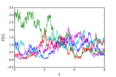
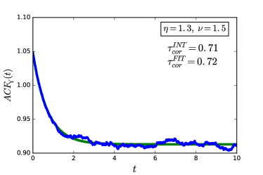
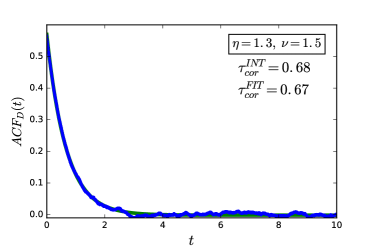
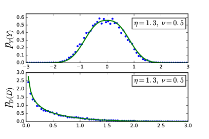
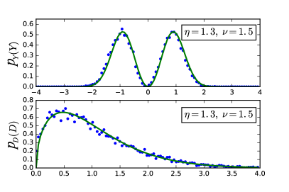
We know from previous studies of DD models that the correlation time of the random diffusivity represents a key factor in the study of the particle dynamics. The correlation time $\tau_{c}$ is evaluated both by means of a two-parametric numerical fit to the exponential function and through the integral

$$\tau_{c}\sim\frac{1}{\mathrm{ACF}(0)}\int_{0}^{\infty}\mathrm{ACF}(\tau)d\tau,$$ (12v)

which is exact for pure exponential autocorrelation functions. The results obtained by the two methods are reported in figure 4 and 5 and they are in excellent agreement, from which we conclude that the diffusivity autocorrelation is exponential to leading order and thus the correlation time $\tau_{c}$ well defined.

It is interesting to notice that the auxiliary function $Y(t)$ in the case of a bimodal distribution possesses a non-zero correlation function in the stationary state. This is due to the fact that despite a vanishing global mean of the PDF, depending on the initial setting each trajectory is representative of only one side of the bimodal PDF.

5 A generalised minimal model for diffusing diffusivities

With the set of equations defined in section 4 we can consider the generalisation of the DD minimal model described in [67], and obtain the process in position space, $X_{\mathrm{DD}}(t)$. Recalling the idea of introducing an analytic description for the dynamics of the random diffusivity, we take that the motion of the particle is defined by the integral version of the overdamped Langevin equation,

$$X_{\mathrm{DD}}(t)=\int_{0}^{t}\sqrt{2D(t^{\prime})}\times\xi(t^{\prime})dt^{\prime},$$ (12w)

where $\xi(t)$ is white Gaussian noise and $D(t)$ is the random time dependent diffusivity obtained in section 4. This dynamics based on the above results for the diffusivity dynamics generalises the idea introduced in [67], where an Ornstein-Uhlenbeck process was selected for the auxiliary variable. Figure 7 shows trajectories obtained from the stochastic equation (12w) where the diffusivity was generated from (12a) with initial conditions taken randomly from the stationary distribution. In ggBM each trajectory has the same $D$ value, while in the DD model the value of $D$ changes as function of time. In turn, individual trajectories of the DD model are quite similar.

Since the DD model is a direct generalisation of the minimal DD model we expect a crossover to a Gaussian displacement PDF for times longer than the correlation time $\tau_{c}$. We thus carry on our analysis for the short and long time regimes separately, before analysing the MSD and kurtosis of this DD process.

Figure 7: Top: Trajectories of the DD model for two different sets of parameters $\nu$ and $\eta$, as indicated in the figure legend and bottom: corresponding time averaged MSDs. In contrast to the behaviour of the ggBM model shown in figure 1, the temporal variation of the diffusivity $D(t)$ is distinct.

5.1 Short time regime

Since the dynamics of the environment is determined by the correlation time $\tau_{c}$ we expect that on short time scales with $t\ll\tau_{c}$ the diffusion coefficient is approximately fixed for each particle and we thus suppose the validity of a superstatistical description at short times (ST),

$$X_{\mathrm{DD}}^{\mathrm{ST}}\sim\sqrt{2D}\int_{0}^{t}\xi(t^{\prime})dt^{\prime}=\sqrt{2D}\times W(t).$$ (12x)

The existence of the superstatistical regime at $t\ll\tau_{c}$ is consistent with the model considered in [67] and with the results reported in [89] concerning the modulation of white noise by any stochastic process whose time correlation function decays exponentially. The superstatistical approach allows us to estimate the short time distribution of the particle displacement by means of

$$f^{\mathrm{ST}}_{\mathrm{DD}}(x,t)\sim\int_{0}^{\infty}p_{D}(D)G(x,t|D)dD.$$ (12y)

This representation corresponds to the ggBM scenario established above, which means that we can borrow its results in equations (12adbv) and (9), considering that $f^{\mathrm{ST}}_{\mathrm{DD}}(x,t)\sim f_{\mathrm{ggBM}}(x,t)$.

Figure 8: Short time (a) and long time (b) PDF of the DD model for $\eta=1.3$ and $\nu=0.5$. The solid lines represent the asymptotic behaviour (9) while the dashed lines represent the Gaussian behaviour (12z) expected at sufficiently long times.

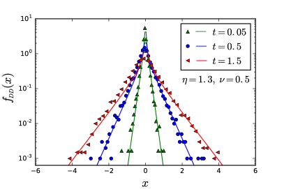
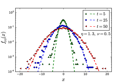
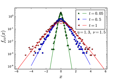
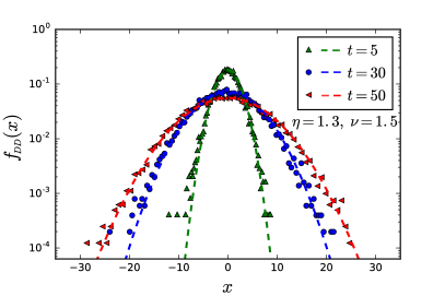
The expected behaviour (9) is confirmed by extensive numerical simulations. Figures 8(a) and 9(a) show the short time PDFs for two different sets of the parameters $\nu$ and $\eta$, and in both cases we observe excellent agreement with the asymptotic behaviour (9).

Comparing figure 2 with figure 8(a) we notice that the ggBM model allows one to describe a process that preserves the exact non-Gaussian PDF, which is exactly the same PDF we obtain in the DD model in the short time regime. Both approaches describe the same superstatistical frame but the DD model then crosses over to a Gaussian beyond the correlation time $\tau_{c}$, see below the discussion of the kurtosis. The establishment of the relation between the DD model and the previously devised ggBM at short times is our third main result.

5.2 Long time regime

At long times (LT), again taking our clue from [67] and from the general results in [89], we expect that eventually a crossover to a Gaussian distribution is observed (as already anticipated in figures 8 and 9). Above the correlation time, that is, for times $t\gg\tau_{c}$ we thus look for a PDF given by

$$f^{\mathrm{LT}}_{\mathrm{DD}}(x,t)\sim\frac{1}{\sqrt{4\pi\langle D\rangle_{\mathrm{stat}}t}}\exp\left(-\frac{x^{2}}{4\langle D\rangle_{\mathrm{stat}}t}\right),$$ (12z)

with the effective diffusivity (11). The numerical results reported in figures 8(b) and 9(b) prove the validity of this behaviour. At sufficient long times the particles have explored all the diffusivity space and a Gaussian behaviour with an effective diffusivity emerges. This leads to a standard Brownian diffusive behaviour. We stress again that the transition from a non-Gaussian to a Gaussian profile depends on the value of the correlation time $\tau_{c}$ of the diffusivity process.

Figure 9: Short time PDF (a) and long time PDF (b) of the DD model for $\eta=1.3$ and $\nu=1.5$. The solid lines represent the asymptotic behaviour in (9) while the dashed lines represent the Gaussian behaviour in (12z) at long times.

5.3 Mean squared displacement

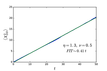
For the DD model we found a crossover of the PDF of the spreading particles. An initial non-Gaussian behaviour is slowly replaced by a Gaussian one. The superstatistical behaviour of the DD approach at short times is equivalent to the ggBM model and is characterised by the non-Gaussianity. Nevertheless, as expected from previous studies [67], the MSD does not change in the course of time and is the same at short and long time regimes. Direct calculation indeed produces the invariant form

$$\langle X_{\mathrm{DD}}^{2}(t)\rangle=2\langle D\rangle_{\mathrm{stat}}t.$$ (12aa)

This continuity of the MSD is demonstrated in figure 10, together with a linear fit proving the validity of the linear trend.

Figure 10: Variance of the DD model. The solid green line represents a linear fit and the corresponding slope is reported in the plot. It is consistent with the expected value $0.40$ according to equation (11).

5.4 Kurtosis

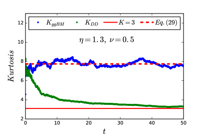
In what follows the second and fourth moments of the non-Gaussian PDF identified in equations (8) and (12y) are studied in terms of the kurtosis that represents one of the first checks for non-Gaussianity. We recall the second order moment calculated in (10) and in a similar way we obtain the fourth order moment

$$\langle X_{\mathrm{ggBM}}^{4}(t)\rangle=\langle X_{\mathrm{DD}}^{4}(t)\rangle_{\mathrm{ST}}=12\langle D^{2}\rangle_{stat}t^{2},$$ (12ab)

where $\langle D^{2}\rangle_{stat}$ is the second moment of the diffusivity in the stationary state. By means of results (10) and (12ab) and recalling the definition of the diffusivity moments in equation (5), the kurtosis $K=\langle x^{4}(t)\rangle/\langle x^{2}(t)\rangle^{2}$ is given by

$$K_{\mathrm{ggBM}} = K_{\mathrm{DD}}^{\mathrm{ST}}=4t^{2}D_{*}^{2}\frac{3\Gamma([\nu+2]/\eta)}{\Gamma(\nu/\eta)}\times\frac{1}{4t^{2}D_{*}^{2}}\left(\frac{\Gamma(\nu/\eta)}{\Gamma([\nu+1]/\eta)}\right)^{2}$$ (12ac)

$$= 3\frac{\Gamma([\nu+2]/\eta)\Gamma(\nu/\eta)}{\Gamma([\nu+1]/\eta)^{2}}>3,$$

for ggBM and the short-time DD process. The non-Gaussian PDF represents a leptokurtic behaviour as can be observed in figure 11, showing the kurtosis of the DD and ggBM models. The value for the kurtosis at short times is in agreement with the value reported in (12ac). At long times the DD kurtosis approaches the value 3 characteristic of the Gaussian distribution, while the ggBM one keeps fluctuating around the same initial value.

Figure 11: Kurtosis of the DD process (green) and ggBM (blue) for 10,000 realisations. For the indicated value of $\eta$ and $\nu$ equation (12ac) yields $K_{\mathrm{ggBM}}\approx 7.74$.

6 Non-equilibrium initial conditions

The results discussed above consider equilibrium initial conditions for the diffusivity fluctuations. In particular, results (10) and (12aa) for the particle MSD exhibit the invariant form $\langle X^{2}(t)\rangle=2\langle D\rangle_{\mathrm{stat}}t$ in both cases. Such equilibrium initial conditions will in general not be fulfilled for particles that are initially seeded in a non-equilibrium environment. For instance, in single particle tracking a tracer bead can be introduced into the system at $t=0$, or similar in computer simulations. After this disturbance the environment equilibrates again. To accommodate for such a case we here study a minimal model for the case of non-equilibrium initial conditions, which leads to another main result of this work. As we are going to see, this non-equilibrium scenario gives rise to differences in the characteristics of the two studied models. In particular, we observe an initial ballistic behaviour. The long time behaviour, of course, does not show differences since in this range the diffusivity reaches its stationary state and we can again consider the results obtained in the previous sections for the long time limit.

We illustrate the role of non-equilibrium conditions by taking a specific, and in fact the simplest, set of parameters, $\nu=0.5$ and $\eta=1$. This defines the stochastic dynamical equation in (12a) as

$$D(t) =Y^{2}(t)$$ (12ada)

$$dY =-\frac{\sigma^{2}}{D_{\star}}Ydt+\sigma dW(t),$$ (12adb)

that corresponds to the well known dynamics of the Ornstein-Uhlenbeck process for the study in [67] with the correlation time $\tau_{c}=D_{\star}/\sigma^{2}$. We start considering the related Fokker-Planck equation

$$\frac{\partial}{\partial t}p(Y,t)=\frac{\sigma^{2}}{D_{\star}}\frac{\partial}{\partial Y}Yp(Y,t)+\frac{\sigma^{2}}{2}\frac{\partial^{2}}{\partial Y^{2}}p(Y,t).$$ (12adae)

We can solve this equation with a non equilibrium condition, for instance, $p(Y,0)=\delta(Y-Y_{0})$, using the method of characteristics in Fourier space. We readily derive the general solution

$$p(Y,t|Y_{0})=\left(\pi D_{\star}[1-\exp(-2t\sigma^{2}/D_{\star})]\right)^{-1/2}\exp\left(-\frac{(Y-Y_{0}\exp(-t\sigma^{2}/D_{\star}))^{2}}{D_{\star}(1-\exp(-2t\sigma^{2}/D_{\star}))}\right).$$ (12adaf)

Recalling relation (12p) for the diffusivity PDF we then obtain

$$p_{D}(D,t|D_{0}=Y_{0}^{2}) = \frac{1}{2\sqrt{D}}\left[p(\sqrt{D},t)+p(-\sqrt{D},t)\right]$$ (12adag)

$$= (4\pi D_{\star}D[1-e^{(}-2t\sigma^{2}/D_{\star})])^{-1/2}$$

$$\times \left\{\exp\left(-\frac{(\sqrt{D}-\sqrt{D_{0}}\exp(-t\sigma^{2}/D_{\star}))^{2}}{D_{\star}(1-\exp(-2t\sigma^{2}/D_{\star}))}\right)\right.$$

$$\left.+\exp\left(-\frac{(-\sqrt{D}-\sqrt{D_{0}}\exp(-t\sigma^{2}/D_{\star}))^{2}}{D_{\star}(1-\exp(-2t\sigma^{2}/D_{\star}))}\right)\right\}.$$

We point out that in the limit of long times this result provides exactly the stationary distribution described in (4) with the specific set of parameters defined above. This is also verified by the trend of the average value

$$\langle D(t)\rangle=\frac{1}{2}\left(D_{\star}(1-e^{-2t\sigma^{2}/D_{\star}})+2D_{0}e^{-2t\sigma^{2}/D_{\star}}\right),$$ (12adah)

in agreement with result (4).

In contrast to the previous analysis, we observe an explicit dependence on time of $p_{D}(D,t)$, which makes the calculations more involved. Thus, we select an initial condition for the diffusivity, $D_{0}=0$, which is convenient for the study of the particles displacement distribution. This leads to a reduction in (12adag), namely,

$$p(D,t|D_{0}=0)=(\pi D_{\star}D(1-\exp(-2t\sigma^{2}/D_{\star})))^{-1/2}\exp\left(\frac{D}{D_{\star}(1-\exp(-2t\sigma^{2}/D_{\star}))}\right).$$ (12adai)

We now study the two models in this particular case of a non-equilibrium initial condition for the diffusivity.

6.1 Diffusing diffusivities with non-equilibrium initial diffusivity condition

The dynamics for the diffusivity encoded in equations (12ada) and (12adb) when choosing the specific set of parameters $\nu=0.5$ and $\eta=1$ is the same as described in [67] when $d=n=1$. Thus, in this paragraph, we extend the description of the minimal DD model studied in [67] to the case of non-equilibrium initial conditions for the diffusivity. In order to proceed with the same notation we introduce dimensionless units for relations (12ada) and (12adb) as well as for the overdamped Langevin equation describing the particle motion [67], such that the full set of stochastic equations reads

$$X_{\mathrm{DD}} =\int_{0}^{t}\sqrt{2D(t^{\prime})}\xi(t^{\prime})dt^{\prime}$$

$$D(t) =Y^{2}(t)$$

$$dY =-Ydt+dW(t).$$ (12adaj)

A subordination approach can then be used to obtain the distribution of the particle displacement [67], namely,

$$f_{DD}(x,t)=\int_{0}^{\infty}T(\tau,t)G(x,\tau)d\tau,$$ (12adak)

where $G(x,\tau)$ is the Gaussian (2) and $T(\tau,t)$ represents the probability density function of the process $\tau(t)=\int_{0}^{t}Y^{2}(t^{\prime})dt^{\prime}$. Starting from the subordination formula (12adak) we obtain the relation

$$\hat{f}_{DD}(k,t)=\tilde{T}(s=k^{2},t)$$ (12adal)

where with the symbols $\hat{\cdot}$ and $\tilde{\cdot}$ we indicate the Fourier and Laplace transforms, respectively. For the particular initial condition $D_{0}=0$, which is equivalent to $y_{0}=0$, the solution is known [99, 100],

$$\tilde{T}(s,t)=\exp\left(\frac{t}{2}\right)\left/\left(\frac{1}{\sqrt{1+2s}}\sinh(t\sqrt{1+2s})+\cosh(t\sqrt{1+2s})\right)^{1/2}\right..$$ (12adam)

This latter quantity is directly related to the MSD of the particles through [67]

$$\langle X^{2}_{\mathrm{DD}}(t)\rangle=-2\left.\frac{\partial\tilde{T}(s,t)}{\partial s}\right|_{s=0}.$$ (12adan)

We readily obtain the closed form result

$$\langle X^{2}_{\mathrm{DD}}(t)\rangle=t-\frac{1}{2}(1-e^{-2t})\sim\left\{\begin{array}[]{ll}t^{2},&t\ll 1\\ t,&t\gg 1\end{array}\right..$$ (12adao)

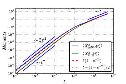
The resulting dynamics is thus no longer Brownian at all times. In contrast, at times shorter than the correlation time (in the dimensionless units used here $\tau_{c}=1$) we obtain a ballistic scaling of the MSD. This behaviour reflects the fact that the diffusivity equilibration in this case with $D_{0}=0$ leads to an initial acceleration.

Starting from equations (12adal) and (12adam) we consider approximations of the PDF for short and long times which, since we are in dimensionless units, correspond to $t\ll 1$ and $t\gg 1$ respectively. In the short time limit, the Fourier transform of the PDF becomes

$$\hat{f}^{ST}_{DD}(k,t)\sim\frac{(1+t+t^{2}/2)^{1/2}}{(1+t+t^{2}/2+k^{2}t^{2})^{1/2}}\sim\frac{1}{t}\left(k^{2}+\frac{1}{t^{2}}\right)^{-1/2}.$$ (12adap)

Note that this expression is normalised, $\hat{f}_{DD}(k=0,t)=1$. After taking the inverse Fourier transform we find

$$f^{ST}_{DD}(x,t) \sim \frac{1}{\pi t}\int_{0}^{\infty}\frac{\cos(kx)}{(k^{2}+1/t^{2})^{1/2}}dk$$ (12adaq)

$$= \frac{1}{\pi t}K_{0}\left(\frac{|x|}{t}\right).$$

Re-establishing dimensional units, this result becomes

$$f^{ST}_{DD}(x,t)\sim\frac{1}{\pi\sigma t}K_{0}\left(\frac{|x|}{\sigma t}\right).$$ (12adar)

Here $K_{\nu}(z)$ is the modified Bessel function of second type. The asymptotic behaviour of this distribution for $|x|\to\infty$ is the Laplace distribution

$$f^{ST}_{DD}(x,t)\sim\frac{1}{\sqrt{2\pi\sigma t|x|}}\exp\left(-\frac{|x|}{\sigma t}\right).$$ (12adas)

In the long time limit equations (12adal) and (12adam) yield

$$\hat{f}^{LT}_{DD}(k,t)\sim\frac{2^{1/2}\exp(t[1-\sqrt{1+2k^{2}}]/2)}{(1+1/\sqrt{1+2k^{2}})^{1/2}},$$ (12adat)

that again is normalised. If we focus on the tails of the distribution in the limit $k\ll 1$ we obtain the Gaussian

$$\hat{f}^{LT}_{DD}(k,t)\sim\exp(-k^{2}t/2)$$ (12adau)

in Fourier space, corresponding to the Gaussian

$$f^{LT}_{DD}(x,t)\sim\frac{1}{\sqrt{2\pi t}}\exp\left(-\frac{x^{2}}{2t}\right)$$ (12adav)

in direct space. Restoring dimensional units and recalling that $\langle D\rangle_{\mathrm{stat}}=D_{\star}/2$, eventually provides

$$f^{LT}_{DD}(x,t) \sim \frac{1}{\sqrt{2\pi D_{\star}t}}\exp\left(-\frac{x^{2}}{2D_{\star}t}\right)$$ (12adaw)

$$= \frac{1}{\sqrt{4\pi\langle D\rangle_{\mathrm{stat}}t}}\exp\left(-\frac{x^{2}}{4\langle D\rangle_{\mathrm{stat}}t}\right),$$

where in the last step we identified the equilibrium value $\langle D\rangle_{\mathrm{stat}}$ of the diffusivity. From the approximations (12adas) and (12adaw) we readily recover the two limiting scaling laws for the variance in equation (12adao).

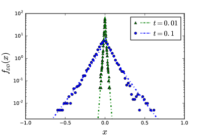
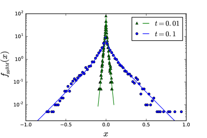
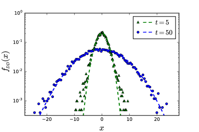
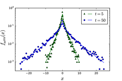
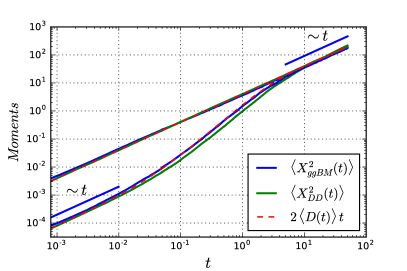
Figure 12 nicely corroborates these findings, comparing the non-equilibrium DD model results for the PDF obtained above with results from stochastic simulations. The crossover behaviour of the associated MSD is displayed in figure 13, again showing very good agreement with the theory.

Figure 12: PDFs of the DD (left) and ggBM (right) models with non-equilibrium initial condition $D_{0}=0$ of the diffusivity. Top: short time behaviour. Bottom: long time behaviour. For the DD model, the dash-dotted lines represent the asymptotic behaviour (12adas) at short times, while the dashed lines are Gaussian fits. For the ggBM model the solid lines represent the analytical result (12adaz).

Figure 13: MSD of the DD model (green) and ggBM (blue). On the left $D_{\star}=1$ and $D_{0}=0$ while on the right we have $D_{\star}=4$ and two different values of $D_{0}$, $D_{0}=\langle D\rangle_{\mathrm{stat}}=D_{\star}/2$ and $D_{0}=0.04$. The first value generates a linear trend of the variance for both models, as we saw for the equilibrium case. In the second case, where $D_{0}\ll D_{\star}$, we observe three regimes. Nice agreement with the analytical results is observed.

6.2 Non-equilibrium generalised grey Brownian motion

The ggBM model discussed in section 3 is based on the static distribution $p_{D}(D)$ of the diffusivity. In order to explore non-equilibrium effects as discussed above for the DD model also within the superstatistical approach, we here propose a non-equilibrium generalisation of the ggBM model. Thus, we generalise the standard ggBM definition (6) and introduce a variability of $D$ in time, according to the stochastic equation

$$X_{\mathrm{ggBM}}(t)=\sqrt{2D(t)}\times W(t).$$ (12adax)

Physically, this new concept may be interpreted as fluctuations of the disjointed environments experienced by the different particles or to temporal changes of the particle size, for instance, due to agglomeration-separation dynamics.

Based on the definition (12adax) it is then straightforward to take the dynamics of $D(t)$ to be the same as the one considered for the DD model. This guarantees that the ensemble properties of this generalised process (12adax) are exactly the same as the ones of the standard ggBM model studied in section 3. In particular, the dependence on time of the diffusivity does not affect the validity of equation (7), so in order to estimate the PDF of the particle displacement of the ggBM model, we consider the distribution (12adai) in the calculation of the integral

$$f_{\mathrm{ggBM}}(x,t|D_{0})=\int_{0}^{\infty}p_{D}(D,t|D_{0})G(x,t|D)dD,$$ (12aday)

which may be defined in general as a dynamic superstatistics because of the dependence of $p_{D}(D,t)$ on $t$. We obtain an explicit solution by means of the Mellin transform following the same procedure as described in Appendix A.2,

$$f_{\mathrm{ggBM}}(x,t|D_{0}=0) = (\pi^{2}D_{\star}t(1-\exp(-2t\sigma^{2}/D_{\star})))^{-1/2}$$ (12adaz)

$$\times K_{0}\left(\frac{|x|}{\sqrt{D_{\star}t(1-\exp(-2t\sigma^{2}/D_{\star}))}}\right),$$

where $K_{\nu}(z)$ is the modified Bessel function of second type. The asymptotic behaviour for $|x|\to\infty$ is given by the exponential

$$f_{\mathrm{ggBM}}(x,t|D_{0}=0)\sim\frac{1}{\sqrt{2\pi|x|\sqrt{D_{\star}t(1-e^{-2t\sigma^{2}/D_{\star}})}}}\exp\left(-\frac{|x|}{\sqrt{D_{\star}t(1-e^{-2t\sigma^{2}/D_{\star}})}}\right).$$ (12adba)

However, in comparison with the result (9) in the equilibrium situation we now observe a different time scaling in the exponent. For short times we see that

$$f_{\mathrm{ggBM}}^{ST}(x,t|D_{0}=0)\sim\frac{1}{\sqrt{\sqrt{2}\pi\sigma t|x|}}\exp\left(-\frac{|x|}{\sqrt{2}\sigma t}\right),$$ (12adbb)

while at long times

$$f_{\mathrm{ggBM}}^{LT}(x,t|D_{0}=0)\sim\frac{1}{\sqrt{2\pi|x|\sqrt{D_{\star}t}}}\exp\left(-\frac{|x|}{\sqrt{D_{\star}t}}\right).$$ (12adbc)

Comparing the short time PDF in (12adbb) with the DD model obtained in (12adas) we notice that they show a difference in the time scaling of a factor $\sqrt{2}$ which is exactly what we observe in figure 12.

Starting from equation (12aday) the MSD can be written as

$$\langle X_{\mathrm{ggBM}}^{2}(t)\rangle =\langle\big{(}\sqrt{2D(t)}W(t)\big{)}^{2}\rangle=2\langle D(t)\rangle t$$ (12adbd)

$$=\left[D_{\star}(1-e^{-2t\sigma^{2}/D_{\star}})+2D_{0}e^{-2t\sigma^{2}/D_{\star}}\right]t.$$

Note that this result is valid for any initial conditions $D_{0}$, not only for the case $D_{0}=0$. As already suggested above, the scaling of the variance is no longer linear at all times. According to the relation between the parameters it is possible to observe the different scaling behaviours

$$\langle X_{\mathrm{ggBM}}^{2}(t)\rangle=\left\{\begin{array}[]{lll}2D_{0}t,&\sigma^{2}t\ll D_{0}\\ 2D_{0}t+2\sigma^{2}t^{2},&D_{0}\ll\sigma^{2}t\ll D_{\star}\\ D_{\star}t&\sigma^{2}t\gg D_{\star}\end{array}\right., 0\leq D_{0}\ll D_{\star},$$ (12adbh)

$$\langle X_{\mathrm{ggBM}}^{2}(t)\rangle=\left\{\begin{array}[]{ll}2D_{0}t-4\sigma^{2}(D_{0}/D_{\star})t^{2}&\sigma^{2}t\ll D_{\star}\\ D_{\star}t&\sigma^{2}t\gg D_{\star}\end{array}\right. \quad\mathrm{elsewhere.}$$ (12adbk)

Thus when $D_{0}\ll D_{\star}$ we observe three regimes for the MSD. When $D_{0}=0$ or when the relation $D_{0}\ll D_{\star}$ does not hold we directly observe an initial ballistic behaviour followed by the stationary linear trend. This behaviour is nicely corroborated in figure 13.

7 Conclusions

A growing range of systems is being revealed which exhibit Brownian yet non-Gaussian diffusion dynamics. Often, an exponential (Laplace) shape of the displacement PDF is observed, however, also stretched Gaussian shapes have been reported. The comparison of diffusion processes recorded by new experimental techniques suggests that the complexity and inhomogeneity of the medium, interpreted as the cause of non-Gaussian behaviour, may influence the spreading of particles in specific fashion and at different levels. In particular, experiments have demonstrated that a non-Gaussian dynamic may persist throughout the observation window and that there are systems that, instead, at long times, exhibit a crossover to Gaussian diffusion. In this article we introduced an analytic approach to generate a random and time-dependent diffusivity with specific features and we proposed two possible models for the spreading dynamics of particles in complex systems: one belonging to the class of generalised grey Brownian motion (ggBM) and the other supporting the idea of diffusing diffusivities (DD).

We saw that the two models have in common the idea that the non-Gaussianity of the PDF is a direct consequence of an inhomogeneity of the environment, represented by a population of diffusivities. The same PDF for the random diffusivity was introduced for both models. We defined an operative set of dynamic stochastic equations to study random diffusivity effects within the broad class of generalised Gamma distributions. This includes the Gamma distribution, or the exponential PDF which produces the Laplace distribution for the particle displacements.

We observed that the main difference between the ggBM and the DD model is the description of the particle dynamics in the long time regime, corresponding to different physical scenarios for the environment. GgBM does not consider an active dynamics of the environment, and the characteristic that mainly influences the particle motion is the randomness of the medium. This means that the statistical features of the medium completely drive the particles in their entire motion. In contrast the DD model supports the idea of diffusing diffusivities considering a dynamics also for the environment. In this way the particles evolve experiencing both a continuous variability in time and a stochasticity in the ensemble. The first model delineates a specific non-Gaussian dynamics for the entire diffusion process, while the second allows to describe a transition from a non-Gaussian to a Gaussian diffusion. In fact, it was shown that the short time non-Gaussian dynamics is the same in the two models, whereas at longer times the ggBM model retains the diffusivity distribution and the DD model leads to an effective value for the diffusivity.

We here also studied the influence of non-equilibrium initial conditions for the diffusivity dynamics and found two main effects. First, the non-equilibrium case breaks the equivalence of the DD and the ggBM models at short times and, second, it causes changes in the temporal evolution of the MSD. In this case the ggBM model, which we showed to represent a stochastic interpretation of superstatistical Brownian motion, describes what we may call a dynamical superstatistics that leads to the presence of different time scaling regimes in the process. The DD model, which we investigated in this case via a subordination approach, at short times can no longer be described through a superstatistic approximation, since the subordination results in that regime diverge from the behaviour of ggBM. Furthermore we observed different time scaling regimes for the DD model, as well. Nevertheless, we note that for both models we never obtained an anomalous time scaling for the MSD, only a crossover between ballistic and linear (Brownian or Fickean) behaviour. In the long time regime we obtained a description of the two models which is in agreement with the one for the equilibrium case, as it should be.

It will be interesting to generalise the present findings to anomalous dynamics with stochastic diffusivity by implementing different types of noise. Maintaining the same population of diffusivities the results obtained for the PDF of the particle displacement will not be affected, yet the MSD scaling will become anomalous.

Appendix A Computation of the superstatistical integral

In this Appendix we provide different methods to solve the integral representing the non-Gaussian PDF of the two models discussed in this work,

$$\bar{P}(x,t)=\int_{0}^{\infty}p_{D}(D)G(x,t|D)dD,$$ (12adbl)

where $G(x,t|D)$ represents a Gaussian distribution and $p_{D}(D)$ is the generalised Gamma distribution (4).

A.1 Computation via Fox $H$-function

Recalling equation (12adbl) we have

$$\bar{P}(x,t) = \int_{0}^{\infty}\frac{\eta}{D^{\nu}_{\star}\Gamma(\nu/\eta)}D^{\nu-1}e^{-(D/D_{\star})^{\eta}}\frac{1}{\sqrt{4\pi Dt}}e^{-\frac{x^{2}}{4Dt}}dD$$ (12adbm)

$$= \frac{\eta}{D^{\nu}_{\star}\Gamma(\nu/\eta)\sqrt{4\pi t}}\int_{0}^{\infty}D^{\nu-3/2}e^{-D^{\eta}}e^{-\lambda D_{\star}/D}dD,$$

where we set $\lambda=x^{2}/4D_{\star}t$. Changing the variable of integration to $y=(D/D_{\star})^{\eta}$ we get

$$\bar{P}(x,t) = \frac{\eta}{\Gamma(\nu/\eta)\sqrt{4\pi D_{\star}t}}\int_{0}^{\infty}y^{\frac{\nu-3/2}{\eta}}e^{-y}e^{-\lambda y^{-1/\eta}}\frac{1}{\eta}y^{\frac{1}{\eta}-1}dy$$ (12adbn)

$$= \frac{1}{\Gamma(\nu/\eta)\sqrt{4\pi D_{\star}t}}\int_{0}^{\infty}y^{-1-(1/2-\nu)/\eta}e^{-y-\lambda y^{-1/\eta}}dy.$$

With the identification

$$e^{-z}=H^{1,0}_{0,1}\left[z\left|\begin{array}[]{l}\rule[3.98337pt]{28.45274pt}{0.56917pt}\\ (0,1)\end{array}\right.\right]$$ (12adbo)

with the Fox $H$-function and exploiting some (very convenient) properties of the $H$-function [101] we then obtain

$$\bar{P}(x,t)=\frac{1}{\Gamma(\nu/\eta)\sqrt{4\pi D_{\star}t}}H^{2,0}_{0,2}\left[\lambda\left|\begin{array}[]{l}\rule[3.98337pt]{28.45274pt}{0.56917pt}\\ ((\nu-1/2)/\eta,1/\eta)(0,1)\end{array}\right.\right].$$ (12adbp)

The Fox function is defined as a generalised Mellin-Barnes integral and has very convenient properties under integral transformations. The Fox function comprises a large range of special functions, including Mejer’s $G$-function, hypergeometric functions, or Bessel functions [102]. In the notation used here the vertical line separates the argument from the function’s parameters, and the horizontal line denotes the lack of upper parameters [102].

Recalling that $\lambda=x^{2}/4D_{\star}t$, we finally obtain

$$\bar{P}(x,t) = \frac{1}{\Gamma(\nu/\eta)\sqrt{4\pi D_{\star}t}}H^{2,0}_{0,2}\left[\frac{x^{2}}{4D_{\star}t}\left|\begin{array}[]{l}\rule[3.98337pt]{28.45274pt}{0.56917pt}\\ ((\nu-1/2)/\eta,1/\eta)(0,1)\end{array}\right.\right]$$ (12adbv)

$$= \frac{1}{\Gamma(\nu/\eta)\sqrt{4\pi D_{\star}t}}\left(\frac{x^{2}}{4D_{\star}t}\right)^{\nu-1/2}$$

$$\times H^{2,0}_{0,2}\left[\frac{x^{2}}{4D_{\star}t}\left|\begin{array}[]{l}\rule[3.98337pt]{28.45274pt}{0.56917pt}\\ (0,1/\eta)(-\nu+1/2,1)\end{array}\right.\right].$$

The series expansion of this function reads [102]

$$H^{2,0}_{0,2}\left[z\left|\begin{array}[]{l}\rule[3.98337pt]{28.45274pt}{0.56917pt}\\ (0,1/\eta)(-\nu+1/2,1)\end{array}\right.\right] = \sum_{n=0}^{\infty}\frac{(-1)^{n}}{n!}\Gamma(1/2-\nu-\eta n)\eta z^{\eta n}$$ (12adbz)

$$+\sum_{n=0}^{\infty}\frac{(-1)^{n}}{n!}\Gamma\left(\frac{\nu-1/2-n}{\eta}\right)z^{1/2-\nu+n}.$$

The asymptotic behaviour is then obtained in the form [102]

$$f_{\mathrm{DD}}^{\mathrm{ST}}(x,t)\sim\frac{1}{\Gamma(\nu/\eta)\sqrt{4\pi D_{\star}t}}\left(\frac{x^{2}}{4D_{\star}t}\right)^{\frac{2\nu-\eta-1}{2(\eta+1)}}\exp\left(-\frac{\eta+1}{\eta}\eta^{\frac{1}{\eta+1}}\left(\frac{x^{2}}{4D_{\star}t}\right)^{\eta/(\eta+1)}\right),$$ (12adca)

for $|x|\to\infty$.

A.2 Computation via Mellin transform

It is possible to rearrange the integral in equation (12adbl) as a convolution integral,

$$\bar{P}(x,t) = \int_{0}^{\infty}p_{D}(D)\frac{\exp(-\frac{(x/\sqrt{t})^{2}}{4D})}{\sqrt{4\pi t}\sqrt{D}}dD$$ (12adcb)

$$= \frac{2}{\sqrt{4t}}\int_{0}^{\infty}\sqrt{D}p_{D}((\sqrt{D})^{2})\frac{\exp(-\frac{(x/\sqrt{D})^{2}}{4})}{\sqrt{\pi}}\frac{d\sqrt{D}}{\sqrt{D}}$$

$$= \frac{1}{\sqrt{4t}}\int_{0}^{\infty}2\xi p_{D}(\xi^{2})M_{1/2}\left(\frac{\bar{x}}{\xi}\right)\frac{d\xi}{\xi},$$

where we defined $\bar{x}=x/t^{1/2}$ and $\xi=D^{1/2}$, and $M_{1/2}$ denotes the $M$-Wright function with parameter $\beta=1/2$ [78]. Considering the convolution formula for the Mellin transform

$$\int_{0}^{\infty}f(\xi)g\left(\frac{x}{\xi}\right)\frac{d\xi}{\xi}\quad\overset{\mathcal{M}}{\longleftrightarrow}\quad f^{M}(s)g^{M}(s),$$ (12adcc)

and remembering the property

$$x^{\beta}f(ax^{h})\quad\overset{\mathcal{M}}{\longleftrightarrow}\quad h^{-1}a^{-(s+\beta)/h}f^{M}\left(\frac{s+\beta}{h}\right),$$ (12adcd)

we compute the Mellin transform of the obtained integral in equation (12adcb), recovering

$$\sqrt{4t}\bar{P}(\bar{x}) =\int_{0}^{\infty}2\xi p_{D}(\xi^{2})M_{1/2}\left(\frac{\bar{x}}{\xi}\right)\frac{d\xi}{\xi}$$ (12adce)

$$\overset{\mathcal{M}}{\longleftrightarrow}p^{M}_{D}\left(\frac{s+1}{2}\right)M^{M}_{1/2}(s).$$

The Mellin transforms for the $M$-Wright function [78] and the generalised Gamma distribution [102] are known and given by

$$M_{\beta}(x) \overset{\mathcal{M}}{\longleftrightarrow} \frac{\Gamma(s)}{\Gamma(1+(s-1)/\beta)},$$

$$\gamma_{(\nu,\eta)}^{gen}(x) \overset{\mathcal{M}}{\longleftrightarrow} D_{\star}^{s-1}\frac{\Gamma((\nu+s-1)/\eta)}{\Gamma(\nu/\eta)}.$$ (12adcf)

We can thus rewrite equation (12adce) in the form

$$p^{M}_{D}\left(\frac{s+1}{2}\right)M^{M}_{1/2}(s) = D_{\star}^{\frac{s-1}{2}}\frac{\Gamma\left(\frac{\nu+(s+1)/2-1}{\eta}\right)}{\Gamma\left(\frac{\nu}{\eta}\right)}\frac{\Gamma(s)}{\Gamma\left(1+\frac{1}{2}(s-1)\right)}$$

$$= \frac{2D_{\star}^{\frac{s-1}{2}}}{\Gamma\left(\frac{\nu}{\eta}\right)}\frac{\Gamma\left(\frac{\nu-1/2+s/2}{\eta}\right)\Gamma(s-1)}{\Gamma\left(\frac{s-1}{2}\right)}$$

$$= \frac{2D_{\star}^{\frac{s-1}{2}}}{\Gamma\left(\frac{\nu}{\eta}\right)}\frac{\Gamma\left(\frac{\nu-1/2+s/2}{\eta}\right)\Gamma\left((s-1)/2+1/2\right)}{2^{1-(s-1)}\sqrt{\pi}}$$

$$= \frac{1}{2\sqrt{D_{\star}\pi}\Gamma\left(\frac{\nu}{\eta}\right)}\left(\frac{1}{4D_{\star}}\right)^{-s/2}\Gamma\left(\frac{\nu-1/2}{\eta}+\frac{s/2}{\eta}\right)\Gamma\left(\frac{s}{2}\right).$$ (12adch)

Now we notice that the Mellin transform of the $H$-function is [102]

$$H_{p,q}^{m,n}\left[ax\left|\begin{array}[]{l}(a_{p},A_{p})\\ (b_{q},B_{q})\end{array}\right.\right]\overset{\mathcal{M}}{\longleftrightarrow}a^{-s}\frac{\left(\prod_{j=1}^{m}\Gamma(b_{j}+B_{j}s)\right)\left(\prod_{j=1}^{n}\Gamma(1-a_{j}-A_{j}s)\right)}{\left(\prod_{j=m+1}^{q}\Gamma(1-b_{j}-B_{j}s)\right)\left(\prod_{j=n+1}^{p}\Gamma(a_{j}+A_{j}s)\right)}.$$ (12adci)

Thus, recalling also the property of the Mellin transform in equation (12adcd) we obtain that

$$\sqrt{4t}\bar{P}(\bar{x})=\frac{1}{\Gamma\left(\nu/\eta\right)\sqrt{\pi D_{\star}}}H_{0,2}^{2,0}\left[\frac{\bar{x}^{2}}{4D_{\star}}\left|\begin{array}[]{l}\rule[3.98337pt]{28.45274pt}{0.56917pt}\\ (\frac{\nu-1/2}{\eta},\frac{1}{\eta})(0,1)\end{array}\right.\right],$$ (12adcj)

and finally

$$\bar{P}(x,t)=\frac{1}{\Gamma\left(\nu/\eta\right)\sqrt{4\pi D_{\star}t}}H_{0,2}^{2,0}\left[\frac{x^{2}}{4D_{\star}t}\left|\begin{array}[]{l}\rule[3.98337pt]{28.45274pt}{0.56917pt}\\ (\frac{\nu-1/2}{\eta},\frac{1}{\eta})(0,1)\end{array}\right.\right].$$ (12adck)

The result here recovered is consistent with equation (12adbv).

A.3 Asymptotic trend via Laplace method

Starting again from equation (12adbl) it is also possible to calculate directly the asymptotic behaviour through the Laplace method. We introduce the new variable $y=D_{\star}/D$ in equation (12adbl),

$$\bar{P}(x,t) = \frac{\eta}{D^{\nu}_{\star}\Gamma(\nu/\eta)\sqrt{4\pi t}}\int_{0}^{\infty}D^{\nu-3/2}e^{-(D/D_{\star})^{\eta}}e^{-\lambda D_{\star}/D}dD$$ (12adcl)

$$= \frac{\eta}{\Gamma(\nu/\eta)\sqrt{4\pi D_{\star}t}}\int_{0}^{\infty}y^{-\nu-1/2}e^{-y^{-\eta}-\lambda y}dy$$

Now the integral looks like a Laplace integral of the form

$$I(\lambda)=\int_{0}^{\infty}f(y)e^{-\lambda y}dy.$$ (12adcm)

In order to apply the Laplace method we need $f(0)\neq 0$ which is not our case since $f(0)=0$ together with all its derivatives. Thus, to evaluate the asymptotics, we define the maximum of the function,

$$\phi(y)=-\lambda y-y^{-\eta},$$ (12adcn)

which is located at $y_{m}=(\eta/\lambda)^{1/\eta+1}$. Introducing of the new variable $\bar{z}=z\eta^{\frac{1}{\eta+1}}$ the integral becomes

$$I(\lambda) = \lambda^{\frac{2\nu-1}{2(\eta+1)}}\int_{0}^{\infty}\bar{z}^{\frac{2\nu-1}{2(\eta+1)}}\exp\left[-\lambda^{\frac{\eta}{\eta+1}}(\bar{z}^{-\eta}+\bar{z})\right]d\bar{z}$$ (12adco)

$$= \lambda^{\frac{2\nu-1}{2(\eta+1)}}\int_{0}^{\infty}\bar{z}^{\frac{2\nu-1}{2(\eta+1)}}e^{\bar{\lambda}f(\bar{z})}d\bar{z},$$

where we defined $f(\bar{z})=-\bar{z}-\bar{z}^{-\eta}$ and $\bar{\lambda}=\lambda^{\eta/(\eta+1)}$. Now the standard Laplace method can be applied considering that the function $f(\bar{z})$ reaches its maximum at $\bar{z}_{m}=\eta^{1/(\eta+1)}$, such that

$$I(\lambda) = \lambda^{\frac{2\nu-1}{2(\eta+1)}}\bar{z}_{m}^{\frac{2\nu+1}{2(\eta+1)}}e^{\bar{\lambda}f(\bar{z}_{m})}\sqrt{\frac{2\pi}{\bar{\lambda}|f^{\prime\prime}(\bar{z}_{m})|}}$$ (12adcp)

$$= \sqrt{\frac{2\pi}{\eta+1}}\eta^{\frac{2\nu+\eta+1}{2(\eta+1)^{2}}}\lambda^{\frac{2\nu-\eta-1}{2(\eta+1)}}\exp\left[-\frac{\eta+1}{\eta}\eta^{\frac{1}{\eta+1}}\lambda^{\frac{\eta}{\eta+1}}\right].$$

This finally leads to

$$\bar{P}(x,t)\simeq\frac{\eta^{\frac{2\nu+\eta+1}{2(\eta+1)^{2}}+1}}{\Gamma(\nu/\eta)\sqrt{4\pi D_{\star}t}}\sqrt{\frac{2\pi}{\eta+1}}\left(\frac{x^{2}}{4D_{\star}t}\right)^{\frac{2\nu-\eta-1}{2(\eta+1)}}\exp\left[-\frac{\eta+1}{\eta}\eta^{\frac{1}{\eta+1}}\left(\frac{x^{2}}{4D_{\star}t}\right)^{\frac{\eta}{\eta+1}}\right],$$ (12adcq)

for $|x|\to\infty$. This result is, up to a numerical prefactor, identical to the asymptotic behaviour obtained in (A.1).

References

- [1] Brown R 1828 A Brief Account of Microscopical Observations Made on the Particles Contained in the Pollen of Plants Phil. Mag. 4 161.
-
[2]
Perrin J 1908 L’agitation moléculaire et
le mouvement brownien Compt. Rend. 146 967.
Perrin J 1909 Mouvement brownien et réalité moléculaire Ann. Chim. Phys. 18 5. - [3] Nordlund I 1914 A New Determination of Avogadro’s Number from Brownian Motion of Small Mercury Spherules Z. Phys. Chem. 87 40.
- [4] Kappler E 1931 Versuche zur Messung der Avogadro-Loschmidtschen Zahl aus der Brownschen Bewegung einer Drehwaage Ann. Phys. (Leipzig) 11 233.
- [5] Einstein A 1905 Über die von der molekularkinetischen Theorie der Wärme geforderte Bewegung von in ruhenden Flüssigkeiten suspendierten Teilchen Ann. Phys. 322 549.
- [6] Sutherland W 1905 A Dynamical Theory of Diffusion for Non-elecrolytes and the Molecoular Mass of Albumin Phil. Mag. 9 781.
- [7] von Smoluchowski M 1906 Zur kinetischen Theorie der Brownschen Molekularbewegung und der Suspensionen Ann. Phys. 21 756.
- [8] Langevin P 1908 Sur la théorie de movement brownien C.R. Hebd. Seances Acad. Sci. 146 530.
- [9] van Kampen N G 1981 Stochastic Processes in Physics and Chemistry (North Holland Publishing Company, Amsterdam).
- [10] Richardson L F 1926 Atmospheric diffusion shown on a distance-neighbour graph Proc. Roy. Soc. London A 110, 709.
- [11] Metzler R & Klafter J 2004 The Restaurant at the End of the Random Walk: Recent Developments in the Description of Anomalous Transport by Fractional Dynamics J. Phys. A 37 R161.
- [12] Scher H & Montroll E W 1975 Anomalous transit-time dispersion in amorphous solids Phys. Rev. B 12 2455.
- [13] Höfling F & Franosch T 2013 Anomalous transport in the crowded world of biological cells Rep. Prog. Phys. 76 046602.
- [14] Nørregaard K, Metzler R, Ritter C M, Berg-Sørensen K & Oddershede L B 2017, Manipulation and Motion of Organelles and Single Molecules in Living Cells Chem. Rev. 117 4342–4375.
- [15] Weiss M, Elsner M, Kartberg F & Nilsson T 2004 Anomalous subdiffusion is a measure for cytoplasmic crowding in living cells Biophys J. 87 3518–24.
- [16] Caspi A, Granek R & Elbaum M 2000 Enhanced Diffusion in Active Intracellular Transport Phys. Rev. Lett. 85 5655–8.
- [17] Seisenberger G, Ried M U, Endreß T, Büning H, Hallek M & Bräuchle C 2001 Real-time single-molecule imaging of the infection pathway of an adeno-associated virus Science 294 1929–32.
- [18] Golding I & Cox E C 2006 Physical Nature of Bacterial Cytoplasm Phys. Rev. Lett. 96 098102.
- [19] Jeon J H, Tejedor V, Burov S, Barkai E, Selhuber-Unkel C, Berg-Sørensen K, Oddershede L & Metzler R 2011, In Vivo Anomalous Diffusion and Weak Ergodicity Breaking of Lipid Granules Phys. Rev. Lett. 106 048103.
- [20] Banks D S & Fradin C 2005 Anomalous diffusion of proteins due to molecular crowding Biophys. J. 89 2960–71.
- [21] Wong I Y, Gardel M L, Reichman D R, Weeks E R, Valentine M T, Bausch A R &Weitz D A 2004 Anomalous diffusion probes microstructure dynamics of entangled F-actin networks Phys. Rev. Lett. 92 178101.
- [22] Szymanski J & Weiss M 2009 Elucidating the Origin of Anomalous Diffusion in Crowded Fluids Phys. Rev. Lett. 103 038102.
- [23] Jeon J-H, Leijnse N, Oddershede L B & Metzler R 2013 Anomalous diffusion and power-law relaxation of the time averaged mean square displacement in worm-like micellar solution New J. Phys. 15 045011.
- [24] Weiss M, Hashimoto H & Nilsson T 2003 Anomalous protein diffusion in living cells as seen by fluorescence correlation spectroscopy Biophys. J. 84 4043–52.
- [25] Weigel A V, Simon B, Tamkun M M & Krapf D 2011 Ergodic and nonergodic processes coexist in the plasma membrane as observed by single-molecule tracking Proc. Natl. Acad. Sci. USA 108 6438–43.
- [26] Manzo C, Torreno-Pina J A, Massignan P, Lapeyre Jr G J, Lewenstein M & Garcia Parajo M F 2015 Weak Ergodicity Breaking of Receptor Motion in Living Cells Stemming from Random Diffusivity Phys. Rev. X 5 011021.
- [27] Kneller G 2014 Communication: A scaling approach to anomalous diffusion J. Chem Phys. 141 041105.
- [28] Jeon J-H, Martinez-Seara Monne H , Javanainen M & Metzler R 2012 Anomalous Diffusion of Phospholipids and Cholesterols in a Lipid Bilayer and its Origins Phys. Rev. Lett. 109 188103.
- [29] Jeon J-H, Javanainen M, Martinez-Seara H, Metzler R & Vattulainen I 2016 Protein crowding in lipid bilayers gives rise to non-Gaussian anomalous lateral diffusion of phospholipids and proteins Phys. Rev. X 6, 021006.
- [30] Metzler R, Jeon J-H & Cherstvy A G 2016 Non-Brownian diffusion in lipid membranes: experiments and simulations Biochimica et Biophysica Acta - Biomembranes 1858 2451–2467.
- [31] Hu X, Hong L, Smith M D, Neusius T, Cheng X & Smith J C 2016 The dynamics of single protein molecules is non-equilibrium and self-similar over thirteen decades in time Nature Physics 12 171–174.
- [32] Robert D, Nguyen T H, Gallet F & Wilhelm C 2010 In vivo determination of fluctuating forces during endosome trafficking using a combination of active and passive microrheology PLoS ONE 4 e10046.
- [33] Reverey J F, Jeon J-H, Leippe M, Metzler R & Selhuber-Unkel C 2015 Superdiffusion dominates intracellular particle motion in the supercrowded cytoplasm of pathogenic Acanthamoeba castellanii Sci. Rep. 5 11690.
- [34] Hughes B D 1995 Random walks and random environments, vol 1: random walks (Oxford University Press, Oxford, UK).
- [35] Metzler R, Jeon J H, Cherstvy A G & Barkai E 2014 Anomalous Diffusion Models and Their Properties: Non-stationarity, Non-ergodicity and Ageing at the Centenary of Single Particle Tracking Phys.Chem. Chem. Phys. 16 24128–24164.
[36]
Schulz J H P, Barkai E & Metzler R 2013 Aging Effects and Population Splitting in Single-Particle Trajectory Averages Phys. Rev. Lett. 110 020602
Schulz J H P, Barkai E & Metzler R 2014 Aging Renewal Theory and Application to Random Walks Phys. Rev. X 4 011028. - [37] Cherstvy A G, Chechkin A V & Metzler R 2013 Anomalous diffusion and ergodicity breaking in heterogeneous diffusion processes New J. Phys. 15 083039.
- [38] Cherstvy A G & Metzler R 2014 Nonergodicity, fluctuations, and criticality in heterogeneous diffusion processes Phys. Rev. E 90 012134.
- [39] Cherstvy A G, Chechkin A V & Metzler R 2014 Ageing and confinement in non-ergodic heterogeneous diffusion processes J. Phys. A: Math. Theor. 47 485002.
- [40] Massignan P, Manzo C, Torreno-Pina J A, García-Parako M F, Lewenstein M & Lapeyre Jr G L 2014 Nonergodic Subdiffusion from Brownian Motion in an Inhomogeneous Medium Phys. Rev. Lett. 112 150603.
- [41] Lutz E 2001 Fractional Langevin equation Phys. Rev. E 64 051106.
- [42] Goychuk I 2009 Viscoelastic subdiffusion: From anomalous to normal Phys. Rev. E 80 046125; Goychuk I 2012 Viscoelastic subdiffusion: Generalized Langevin equation approach Adv. Chem. Phys. 150 187–253.
- [43] Mandelbrot B B & van Ness J W 1968, Fractional Brownian motions, fractional noises and applications SIAM Review 10 422–437.
- [44] Deng W & Barkai E 2009 Ergodic properties of fractional Brownian-Langevin motion Phys. Rev. E 79 011112.
- [45] Schwarzl M, Godec A & Metzler R 2107 Quantifying non-ergodicity of anomalous diffusion with higher order moments Sci Rep. 7 3878.
- [46] Jeon J-H & Metzler R 2012 Inequivalence of time and ensemble averages in ergodic systems: Exponential versus power-law relaxation in confinement Phys. Rev. E 85 021147.
- [47] Wang B, Kuo J, Bae S C & Granick S 2012 When Brownian Diffusion Is Not Gaussian Nat. Mater. 11 481–5.
- [48] Wang B, Antony S M, Bae S C & Granick S 2009 Anomalous Yet Brownian Proc. Nat. Acad, Sci. U.S.A. 106 15160–15164.
- [49] Leptos K C, Guasto J S, Gollub J P, Pesci A I & Goldstein R E 2009 Dynamics of Enhanced Tracer Diffusion in Suspensions of Swimming Eukaryotic Microorganisms Phys. Rev. Lett. 103 198103.
- [50] Xue C, Zheng X, Chen K, Tian Y & Hu G 2016 Probing Non-Gaussianity in Confined Diffusion of Nanoparticles J. Phys. Chem. Lett. 7 514–9.
- [51] Wang D, Hu R, Skaug M J & Schwartz D K 2015 Temporally Anticorrelated Motion of Nanoparticles at a Liquid Interface J. Phys. Chem. Lett. 6 54–9.
- [52] Dutta S & Chakrabarti J 2016 Anomalous dynamical responses in a driven system EPL 116 38001.
- [53] Hapca S, Crawford J W & Young I M 2009 Anomalous Diffusion of Heterogeneous Populations Characterized by Normal Diffusion at The Individual Level J. R. Soc. Interface 6 111–22.
- [54] Cherstvy A G, Günther O, Beta C & Metzler R (unpublished).
- [55] Kob W & Andersen H C 1995 Testing mode-coupling theory for a supercooled binary Leonard-Jones mixture: The van Hove correlation function Phy. Rev. E 51 4626–4641.
- [56] Chaudhuri P, Berthier L & Kob W 2007 Universal Nature of Particle Displacements Close to Glass and Jamming Transitions Phys. Rev. Lett. 99 060604.
- [57] R-Vargas S, Rovigatti L & Sciortino F 2017 Connectivity, dynamics, and structure in a tetrahedral network liquid Soft Matt. 13 514–530.
- [58] Samanta N & Chakrabarti R 2016 Tracer diffusion in a sea of polymers with binding zones: mobile vs. frozen traps Soft Matter 12 8554–8563.
- [59] Skaug M J, Wang L, Ding Y & Schwartz D K 2015 Hindered Nanoparticle Diffusion and Void Accessibility in a Three-Dimensional Porous Medium ACS Nano 9 2148–2156
- [60] Stuhrmann B, Soares e Silva M, Depken M, Mackintosh F C & Koenderink G H 2012 Nonequilibrium fluctuations of a remodeling in vitro cytoskeleton Phys. Rev. E 86 020901.
- [61] Lampo T, Stylianido S, Backlund M P, Wiggins P A & Spakowitz A J 2017 Cytoplasmic RNA-Protein Particles Exhibit Non-Gaussian Subdiffusive behaviour Biophys. J. 112 532–542.
- [62] Soares e Silva M, Stuhrmann B, Betz T & Koenderink G H 2014 Time-resolved microrheology of actively remodeling actomyosin networks New J. Phys. 16 075010.
- [63] Beck C & Cohen EDB 2003 Superstatistics Physica A 322, 267.
- [64] Beck C 2006 Superstatistical Brownian Motion Prog. Theor. Phys. Suppl. 162 29–36.
- [65] van der Straeten E & Beck C 2009 Superstatistical fluctuations in time series: Applications to share-price dynamics and turbulence Phys. Rev. E 80 036108.
- [66] Metzler R 2017 Gaussianity Fair:The Riddle of Anomalous yet Non-Gaussian Diffusion Biophys. J. - New and Notable 112 413–415.
- [67] Chechkin A V, Seno F, Metzler R & Sokolov I 2017 Brownian Yet Non-Gaussian Diffusion: From Superstatistics to Subordination of Diffusing Diffusivities Phys. Rev. X 7 021002.
- [68] van der Straeten E & Beck C 2011 Dynamical modelling of superstatistical complex systems Physica A 390 951–956.
- [69] Ślęzak J & Metzler R 2018 New J. Phys.
- [70] Dubinko V I, Tur A V, Turkin AA & Yanovsky V V 1990 Diffusion in Fluctuative Medium Radiat. Eff. Defects Solid. 112 233–243.
- [71] Albers T & Radons G 2013 Subdiffusive Continuous Time Random Walks and Weak Ergodicity Breaking Analyzed with the Distribution of Generalized Diffusivities Europhys. Lett. 102 40006.
- [72] Rozenfeld R, Luczka J & Talkner P 1998 Brownian Motion in a Fluctuating Medium Phys. Lett. A 249 409–414.
- [73] Luczka J, Talkner P & Hänggi P 2000 Diffusion of Brownian Particles Governed by Fluctuating Friction Physica A 278 18–31.
- [74] Luczka J & Zaborek B 2004 Brownian Motion: A Case of Temperature Fluctuation Acta Phys. Pol. B 35 2151–2164.
- [75] Uneyama T, Miyaguchi T & Akimoto T 2015 Fluctuation Analysis of Time-Averaged Mean-Square Displacement for the Langevin Equation with Time-Dependent and Fluctuating Diffusivity Phys. Rev. E 92 032140.
- [76] Akimoto T & Yamamoto E 2016 Distributional behaviours of Time-Averaged Observables in the Langevin Equation with Fluctuating Diffusivity: Normal Diffusion but Anomalous Fluctuations Phys. Rev. E 93 062109.
- [77] Cherstvy A G & Metzler R 2106 Anomalous diffusion in time-fluctuating non-stationary diffusivity landscapes Phys. Chem. Chem. Phys. 18 23840–23852.
- [78] Mura A, Taqqu M S & Mainardi F 2008 Non-Markovian diffusion equations and processes: Analysis and simulations Physica A 387 5033-5064.
- [79] Mura A & Mainardi F 2009 A class of self-similar stochastic processes with stationary increments to model anomalous diffusion in physics Int. Transf. Spe. Funct. 20 185-198.
- [80] Pagnini G 2012 Erdélyi Kober fractional diffusion Fract. Calc. App. Anal. 5 117-127.
- [81] Mura A & Pagnini G 2008 Characterizations and simulations of a class of stochastic processes to model anomalous diffusion J. Phys. A: Math. Theor. 41 285003.
- [82] Molina-García, Pham TM, Paradisi P & Pagnini P 2016, Fractional kinetics emerging from ergodicity breaking in random media, Phys. Rev. E 94, 052147.
- [83] Chubynsky M V & Slater G W 2014 Diffusing Diffusivities: A Model for Anomalous, Yet Brownian Diffusion Phys. Rev. Lett. 113 098302.
- [84] Tejedor V & Metzler R 2010 Anomalous diffusion in correlated continuous time random walks J. Phys. A 43 082002.
- [85] Magdziarz M, Metzler R, Szczotka W & Zebrowski P 2012 Correlated Continuous Time Random Walks in External Force Fields, Phys. Rev. E 85 051103.
- [86] Matse M, Chubynsky M V & Bechhoefer J 2017 Test of the diffusing-diffusivity mechanism using nearwall colloidal dynamics arXiv:1706.02039v1
- [87] Jain R & Sebastian K L 2016 Diffusion in a Crowded, Rearranging Environment J. Phys. Chem. B 120 3988–92.
- [88] Jain R & Sebastian K L 2017 Diffusing diffusivity: a new derivation and comparison with simulations J. Chem. Sci. 129 929–937.
- [89] Tyagi N & Cherayil B J 2017 Non-Gaussian Brownian Diffusion in Dynamically Disordered Thermal Environments J. Phys. Chem. B, 121 7204–7209.
- [90] Lanoiselée Y & Grebenkov D 2018 A model of non-Gaussian diffusion in heterogeneous media J. Phys. A, at press, DOI:10.1088/1751-8121/aab15f.
- [91] Beck C 2006 Stretched exponentials from superstatistics Physica A 365, 96.
- [92] Javanainen M, Hammaren H, Monticelli L, Jeon J-H, Miettinen M S, Martinez-Seara H, Metzler R & Vattulainen I 2013 Anomalous and normal diffusion of proteins and lipids in crowded lipid membranes, Faraday Discuss., 161 397–417.
- [93] Jeon J-H, Javanainen M, Martinez-Seara H, Metzler R & Vattulainen I 2016 Protein Crowding in Lipid Bilayers Gives Rise to Non-Gaussian Anomalous Lateral Diffusion of Phospholipids and Proteins Phys. Rev. X 6 021006.
- [94] Pagnini G & Paradisi P 2016 A stochastic solution with gaussian stationary increments of the symmetric space-time fractional diffusion equation Fract. Calc. Appl. Anal. 19 408–440.
- [95] Thomson D J 1987 Criteria for the selection of stochastic models of particle trajectories in turbulent flows J. Fluid. Mech. 180 529–556.
- [96] Ross S 2010 A first course in probability - 8th edition (Pearson Prentice Hall, USA).
- [97] Heston SL 1993 A Closed-Form Solution for Options with Stochastic Volatility with Applications to Bond and Currency Options Rev. Financ. Studies 6, 327.
- [98] Dragulescu A & Yakovenko V 2002 Probability distribution of returns in the Heston model with stochastic volatility Quantit. Finance 2, 443.
- [99] Liptser R S, & Shiryaev A N 2001 Statistics of Random Processes II (Springer-Verlag Berlin Heidelberg).
- [100] Dankel Jr T 1991 On the distribution of the integrated square of the Ornstein-Uhlenbeck process SIAM J. Appl. Math. 51, 568-574.
- [101] Prudnikov A P 1990 Integrals and series. Volume 3: more special functions (CRC Press).
- [102] Mathai A M & Saxena R K 1978 The -Function with Applications in Statistics and Other Disciplines (Wiley Eastern, New Delhi, India).