Monopulse beam synthesis
using a sparse single-layer of weights

Abstract

A conventional monopulse radar system uses three beams; sum beam, elevation difference beam and azimuth difference beam, which require different layers of weights to synthesize each beam independently. Since the multi-layer structure increases hardware complexity, many simplified structures based on a single layer of weights have been suggested. In this work, we introduce a new technique for finding disjoint and fully covering sets of weight vectors, each of which constitutes a sparse subarray, forming a single beam. Our algorithm decomposes the original non-convex optimization problem for finding disjoint weight vectors into a sequence of convex problems. We demonstrate the convergence of the algorithm and show that the interleaved array structure is able to meet difficult beam constraints.

I Introduction

A monopulse radar with an antenna array needs multiple beams; the sum beam and the delta beams, on a same antenna-array face. This, in turn, requires multiple layers of weights i.e., transmit-receive modules (TRMs) to shape each beam, independently and optimally. However, it is costly and structurally complicated to attach multiple TRMs on each antenna. Therefore, many researchers have engaged in the problem of subarraying and assigning a single weight on each antenna heuristically [1] and systematically  [2, 3, 4, 5, 6, 7, 8, 9].

The first approach is to use multiple and clustered sub-arrays, whose responses are combined to obtain multiple beams [4, 6, 5]. For example, Figure 1(a) shows two clustered non-overlapping subarrays, which form a single-layer of weights, that are used to obtain the sum beam $F_{1}$ and the delta beam $F_{2}$. Each subarray response is generated by combining the antenna responses in analog manner, and each beam response is obtained by combining the subarray responses in digital manner. Figure 1(a) shows non-overlapping subarrays [10], but partially overlapping [11, 12] structures have been studied as well.

(a) An example of clustered non-overlapping subarrays, which form a single-layer of weights. This particular structure is sometimes called the common weight array. In general, the summation of the antenna response is carried out before the analog-digital conversion (ADC) and the summation of the subarray responses, after the ADC.

(b) An example of fully interleaved structure which form a single-layer of weights with sparse and disjoint subarrays. The summation of the antenna responses is carried out before the ADC.

Figure 1: Two types of single-layer monopulse antenna structure.

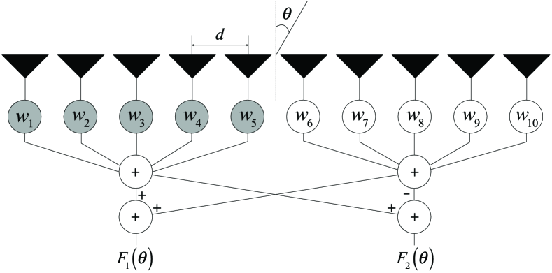
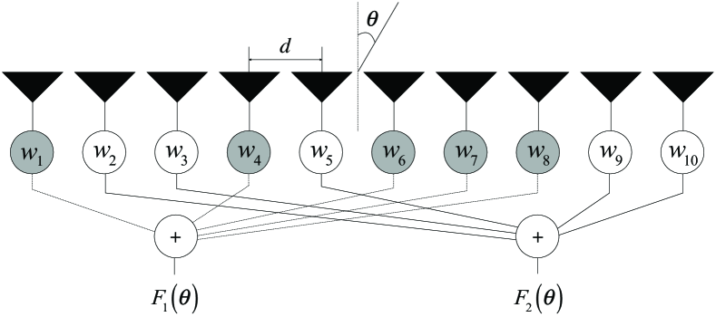
The second approach is to use sparse and irregular subarrays. As an example, the fully interleaved thinned linear array (FITLA) structure [3] is shown in Figure 1(b). The larger aperture of each sparse sub-array, compared with that of a dense array with the same number of weights, gives sharper and narrower beam while the irregularity of the sparse array suppresses grating lobes.

Above mentioned beamforming structures can be synthesized by formulating a constrained minimization problem, which is in general, non-convex. Although this minimization can be carried out with an inefficient global optimization method, two ingeniously crafted methods, the alternating projection method and the hybrid method exist.

The alternating projection method [7, 13, 14, 15, 16, 17] iteratively finds an intersecting point of two sets $\mathcal{M}$ and $\mathcal{B}$, where $\mathcal{M}$ specifies the excitation constraints and $\mathcal{B}$, the beam pattern, by repeatedly projecting the point in a current set onto the other. A difficulty with this method is that one of the two sets, in general, is not convex, and therefore the starting point must be chosen carefully to ensure the convergence to the global minimum. We remark that the alternating projection method appears in a variety of algorithms, sometimes disguisedly, including the direction of arrival finding algorithm [18] and the alternating direction implicit (ADI) method for solving partial differential equations [19].

The hybrid method [4, 6, 2, 5, 7, 8, 9, 20] also decomposes the constrained minimization problem into two; one a convex problem and the other, usually a non-convex problem. This method has been successfully applied to the monopulse beam synthesis by iteratively finding the weights as well as subarray grouping for the structures in Figures 1(a) and 1(b)  [2, 3, 4, 5, 6, 7, 8, 9].

In general, however, both the alternating projection method and the hybrid method involve a non-convex optimization step, and therefore, require a global optimization algorithm [13] or a good choice of the starting point [9].

We propose a new algorithm which solves the original non-convex problem for finding the structure in Figure 1(b) by decomposing it into a sequence of l1-minimization problems, which are convex. In a sense, the proposed algorithm is a variant of the alternating projection method, where the non-convex constraint set is replaced with a more convenient convex set [21].

II Data model

Assuming omni-directional antennas, let us define the array response vector by ${\bf a}(\theta)=[1,e^{-jkdsin\theta},\cdots,e^{-jkd(N-1)sin\theta}]^{T}$, where $j=\sqrt{-1}$, and $k=2\pi/\lambda$. The angle $\theta$ denotes the bearing of a target and the constant $d$, antenna spacing. Then sum beam response $F_{1}$ and delta beam response $F_{2}$ are respectively, expressed as

$${F_{1}}\left({\theta}\right)={\bf{a}}{\left(\theta\right)^{H}}{{\bf{M}}^{H}}{{\bf{w}}_{1}},\quad{\bf w}_{1}\in{\mathbb{C}}^{N\times 1},$$ (1)

$${F_{2}}\left(\theta\right)={\bf{a}}{\left(\theta\right)^{H}}{{\bf{M}}^{H}}{{\bf{w}}_{2}},\quad{\bf w}_{2}\in{\mathbb{C}}^{N\times 1},$$ (2)

where ${\bf{M}}$ represents the mutual coupling matrix. The vectors ${\bf w}_{1}$ and ${\bf w}_{2}$ are disjoint and fully covering weight vectors. For example, for the array in Figure 1(b), we have

$${\bf w}_{1} = [w_{1},0,0,w_{4},0,w_{6},w_{7},w_{8},0,0]^{T},$$ (3)

$${\bf w}_{2} = [0,w_{2},w_{3},0,w_{5},0,0,0,w_{9},w_{10}]^{T}.$$ (4)

The role of weight vectors ${\bf w}_{1}$ and ${\bf w}_{2}$ is to compensate the mutual coupling as well as to shape the beams under the altered array response vector, ${\bf M}{\bf a}(\theta)$.

Let $\Theta_{1}$ and $\Theta_{2}$ be the sets of side-lobe angles of the sum beam and the delta beam, respectively, and $\theta_{0}$, the bore-sight angle. A monopulse radar functions properly, if $F_{1}$ and $F_{2}$ are synthesized to satisfy each beam constraints, i.e., the weight vectors ${\bf w}_{1}$ and ${\bf w}_{2}$ belong to the sets defined by

$${\mathcal{C}_{1}}=\left\{{{{\bf{w}}_{1}}\left|{{F_{1}}\left({{\theta_{0}}}\right)=\mu,\;{{\left|{{F_{1}}\left({{\theta_{1,m_{1}}}}\right)}\right|}^{2}}\leq{\tau_{1}}}\right.}\right\},$$ (5)

$${\mathcal{C}_{2}}=\left\{{{{\bf{w}}_{2}}\left|{\begin{array}[]{*{20}{c}}{{F_{2}}\left({{\theta_{0}}}\right)=0,\;{{\left|{{F_{2}}\left({{\theta_{2,m_{2}}}}\right)}\right|}^{2}}\leq{\tau_{2}},}\\ {{\left.\frac{\partial F_{2}\left(\theta\right)}{{\partial\theta}}\right|}_{\theta=\theta_{0}}={{\mu s}}}\end{array}}\right.}\right\},$$ (6)

where $\{\theta_{1,m_{1}}\}_{m_{1}=1}^{M_{1}}\in\Theta_{1}$ and $\{\theta_{2,m_{2}}\}_{m_{2}=1}^{M_{2}}\in\Theta_{2}$ indicate sampling points in the side-lobe regions. The constants $M_{1}$ and $M_{2}$ represent the number of samples in the side-lobe regions for each beam. Only one sample at $\theta_{0}$ is taken in the main-lobe regions. Here, $\mu$ is defined as the array gain for the sum beam at the bore sight. The bounds $\tau_{1}$ and $\tau_{2}$ denote the maximum side-lobe levels (SLLs) of $F_{1}$ and $F_{2}$, respectively, and the constant $s$ is the slope of $F_{2}$ at the bore sight. The sets ${\mathcal{C}}_{1}$ and ${\mathcal{C}}_{2}$ are convex sets, since $F_{1}$ and $F_{2}$ are linear functions of ${\bf w}_{1}$ and ${\bf w}_{2}$, respectively. See Equation (1) and (2).

III Argumentative reselection algorithm

To find disjoint weight vectors such as ${{\bf{w}}_{1}}$ and ${{\bf{w}}_{2}}$ in Figure 1(b), we shall build an optimization problem and propose an algorithm to solve the problem. We call the process, argumentative reselection algorithm, since the process is comparable to the situation where many people argue for their individual benefit, but eventually reach a compromise with which all can accept.

III-A The problem

Now let us define the two-variable cost function ${\tilde{J}}\left({{{\bf{w}}_{1}},{{\bf{w}}_{2}}}\right)\buildrel\Delta\over{=}{{\left|{{{\bf{w}}_{1}}}\right|}^{T}}\cdot{\left|{{{\bf{w}}_{2}}}\right|}$, where ${\left|\cdot\right|}$ takes the element-wise absolute value. Then the problem is to find ${\bf\hat{w}}_{1}$ and ${\bf\hat{w}}_{2}$ such that

$$\left({\bf\hat{w}}_{1},{\bf\hat{w}}_{2}\right)= \mathop{{\mathop{\rm argmin}\nolimits}}\limits_{{\bf w}_{1},{\bf w}_{2}}{\tilde{J}}\left({\bf w}_{1},{\bf w}_{2}\right)$$ (7)

$${\rm subject}\;{\rm to}\;{{\bf{w}}_{1}}\in{\mathcal{C}_{1}},{{\bf{w}}_{2}}\in{\mathcal{C}_{2}}.$$

The disjoint requirement of ${\bf w}_{1}$ and ${\bf w}_{2}$ is built-into the cost function because if we are able to minimize the cost of ${\tilde{J}}$ down to zero, then we shall obtain a disjoint pair ${\bf w}_{1}\in{\mathcal{C}}_{1}$ and ${\bf w}_{2}\in{\mathcal{C}}_{2}$. Otherwise, there are no disjoint ${\bf w}_{1}\in{\mathcal{C}}_{1}$ and ${\bf w}_{2}\in{\mathcal{C}}_{2}$, and we need to relax the specifications in ${\mathcal{C}}_{1}$ and ${\mathcal{C}}_{2}$. This trial and error approach of the parameter selection is quite common for beam synthesis problems [7].

III-B The algorithm

(a) Magnitude distributions of $\left|{\bf{w}}_{1}\right|$ and $\left|{\bf{w}}_{2}\right|$ after the first iteration.

(b) Magnitude distributions of $\left|{\bf{w}}_{1}\right|$ and $\left|{\bf{w}}_{2}\right|$ after the second iteration.

(c) Magnitude distributions of $\left|{\bf{w}}_{1}\right|$ and $\left|{\bf{w}}_{2}\right|$ after the fourth iteration.

Figure 2: Antenna weight distributions as the argumentative reselection algorithm proceeds.

A difficulty in the above optimization problem is that the two-variable cost function is not convex [22]. However, if one of the weight vectors ${\bf w}_{1}$ and ${\bf w}_{2}$ is constant, then the resulting one-variable cost function $J(\cdot)$ becomes convex. This leads us to build a new algorithm for Problem (7), which utilizes penalizing vectors ${\bf p}_{1}$ and ${\bf p}_{2}$:

Choose random ${\bf w}_{1}$ and ${\bf w}_{2}$;
repeat

1. Set ${\bf p}_{1}\coloneqq\left|{{\bf{w}}}_{2}\right|$ and solve
   ${{{\bf{w}}}_{1}}\coloneqq\mathop{{\mathop{\rm argmin}\nolimits}}\limits_{{{\bf{w}}_{1}}}J({\bf w}_{1},{\bf p}_{1})\;{\rm s.t.}\;{{\bf{w}}_{1}}\in{\mathcal{C}_{1}}$;.

2. Set ${\bf p}_{2}\coloneqq\left|{{\bf{w}}}_{1}\right|$ and solve
   ${{{\bf{w}}}_{2}}\coloneqq\mathop{{\mathop{\rm argmin}\nolimits}}\limits_{{{\bf{w}}_{2}}}J({\bf w}_{2},{\bf p}_{2})\;{\rm s.t.}\;{{\bf{w}}_{2}}\in{\mathcal{C}_{2}}$;

until converge

III-B1 Intuitive analysis of the algorithm

Let us consider the statement (ii) in the above algorithm, where the penalizing vector ${\bf p}_{2}\buildrel\Delta\over{=}[p_{1},p_{2},\cdots,p_{N}]^{T}$ is the result ${\bf w}_{1}$ after (i) in the current iteration, and ${\bf w}_{2}\buildrel\Delta\over{=}[w_{1},w_{2},\cdots,w_{N}]^{T}$ is the result after (ii) in the previous iteration. From

$$J({\bf w}_{2},{\bf p}_{2})=|w_{1}|\cdot p_{1}+|w_{2}|\cdot p_{2}+\cdots+|w_{N}|\cdot p_{N},$$ (8)

the new weight ${\bf w}_{2}$ is to be found by minimizing $J({\bf w}_{2},{\bf p}_{2})$, or in other words, by taking a smaller $w_{i}$ for a larger $p_{i}$. Therefore, the vectors ${\bf w}_{1}$ and ${\bf w}_{2}$ tend to become disjoint as the iteration continues.

Figure 2 shows an example of antenna distributions in the course of the argumentative reselection process. The initial values for the elements of ${\bf w}_{1}$ and ${\bf w}_{2}$ are all $1$s. After the first iteration (See Figure 2(a).), there are $18$ shared antennas by the sum beam and the delta beam. However, as the algorithm proceeds, the shared antennas are removed gradually (See Figure 2(b).), and then completely (See Figure 2(c).).

III-B2 Argumentative reselection algorithm for multiple beams

In the case of $K$ beams, i.e., $K$ weight vectors in the sets $\{{\mathcal{C}}_{k}\}_{k=1}^{K}$, the $K$-variable cost function of the optimization problem is defined as:

$${\tilde{J}}\left({{{\bf{w}}_{1}},{{\bf{w}}_{2}},\cdots,{{\bf{w}}_{K}}}\right)={1\over 2}\sum\limits_{\scriptstyle i,j=1,\hfill\atop\scriptstyle i\neq j\hfill}^{K}{{{\left|{{{\bf{w}}_{i}}}\right|}^{T}}\cdot\left|{{{\bf{w}}_{j}}}\right|}.$$ (9)

If we define the penalizing vectors and the one-variable cost function, respectively as:

$${{\bf{p}}_{k}}=\sum\limits_{\scriptstyle j=1,\hfill\atop\scriptstyle j\neq k\hfill}^{K}{\left|{{{{{\bf w}}}_{j}}}\right|},\quad J({\bf w}_{k},{\bf p}_{k})=|{\bf w}_{k}|^{T}\cdot{\bf p}_{k},$$ (10)

then we have Algorithm 1 below.

Algorithm 1 Algorithm for the argumentative reselection process

initialize ${{{\bf{w}}}_{k}}\coloneqq{{\bf{randn}}(N,1)+j{\bf{randn}}(N,1)}\;{\rm for}\;k\in\left\{{1,\ldots,K}\right\}$, and set ${J^{(0)}}\coloneqq$ inf
for $l=1,2,\cdots$
        for $k=1:K$
              ${{\bf{p}}_{k}}\coloneqq\sum\limits_{\scriptstyle j=1,\hfill\atop\scriptstyle j\neq k\hfill}^{K}{\left|{{{{{\bf w}}}_{j}}}\right|}$;
              ${{{\bf{{w}}}}_{k}}\coloneqq\mathop{{\mathop{\rm argmin}\nolimits}}\limits_{{{\bf{w}}_{k}}}J({\bf w}_{k},{\bf p}_{k}),\;{\rm subject}\;{\rm to}\;{{\bf{w}}_{k}}\in{\mathcal{C}_{k}}$;
        end
       ${J^{(l)}}\coloneqq{\tilde{J}}\left({{{{\bf{w}}}_{1}},{{{\bf{w}}}_{2}},\cdots,{{{\bf{w}}}_{K}}}\right)$;
        if $J^{(l-1)}-J^{(l)}<\epsilon$ exit
end
return ${{\bf{\hat{w}}}_{k}}\coloneqq{{\bf{{w}}}_{k}}\;{\rm for}\;k\in\left\{{1,\ldots,K}\right\};$

The above stated algorithm with two weight vectors is a special case of Algorithm 1, when $K=2$. Now the convergence of Algorithm 1 is proven below.

Theorem: The sequence $J^{(l)}$ in Algorithm 1 is monotonically decreasing and bounded below by zero, and thus convergent.

Proof.

Writing the intermediate results explicitly, let ${\bf w}_{k}^{(l)}$ be the optimal vector obtained after the $k$th inner-iteration of the $l$th outer-iteration, and we define

$$J_{k}^{(l)}\buildrel\Delta\over{=}{\tilde{J}}({\bf w}_{1}^{(l)},{\bf w}_{2}^{(l)},\cdots,{\bf w}_{k}^{(l)},{\bf w}_{k+1}^{(l-1)},\cdots,{\bf w}_{K}^{(l-1)}).$$ (11)

Then when $k=1$,

$${{\bf w}}_{1}^{\left({l+1}\right)} = \mathop{{\mathop{\rm argmin}\nolimits}}\limits_{{{\bf{w}}_{1}}}J({\bf w}_{1},{\bf p}_{1})$$ (12)

$$= \mathop{{\mathop{\rm argmin}\nolimits}}\limits_{{{\bf{w}}_{1}}}{\left|{{{\bf{w}}_{1}}}\right|^{T}}\cdot\left(\sum\limits_{\scriptstyle j=2}^{K}{\left|{{{\bf w}}_{j}^{\left(l\right)}}\right|}\right).$$ (13)

Therefore,

$$J_{1}^{\left({l+1}\right)} ={\left|{{{\bf w}}_{1}^{\left({l+1}\right)}}\right|^{T}}\!\cdot\!\left({\sum\limits_{\scriptstyle j=2}^{K}{\left|{{{\bf w}}_{j}^{\left(l\right)}}\right|}}\right)\!+\!{1\over 2}\sum\limits_{\scriptstyle i,j=2,\hfill\atop\scriptstyle i\neq j\hfill}^{K}{{{\left|{{{\bf w}}_{i}^{\left(l\right)}}\right|}^{T}}\!\cdot\!\left|{{{\bf w}}_{j}^{\left(l\right)}}\right|}$$ (14)

$$\leq{\left|{{{\bf w}}_{1}^{\left(l\right)}}\right|^{T}}\cdot\left({\sum\limits_{\scriptstyle j=2}^{K}{\left|{{{\bf w}}_{j}^{\left(l\right)}}\right|}}\right)+{1\over 2}\sum\limits_{\scriptstyle i,j=2,\hfill\atop\scriptstyle i\neq j\hfill}^{K}{{{\left|{{{\bf w}}_{i}^{\left(l\right)}}\right|}^{T}}\cdot\left|{{{\bf w}}_{j}^{\left(l\right)}}\right|}$$ (15)

$$=J_{K}^{\left(l\right)},$$ (16)

so that $J_{K}^{(l)}\geq J_{1}^{(l+1)}$. Similarly $J_{k}^{(l+1)}\geq J_{k+1}^{(l+1)}$, and therefore $J_{K}^{(l)}\geq J_{K}^{(l+1)}\geq J_{K}^{(l+2)}\geq\cdots$. Now the proof is complete because $J_{K}^{(l)}=J^{(l)},\forall l$, and $J^{(l)}$ are bounded below by zero from the definition of ${\tilde{\it J}}$ in Equation (9). ∎

IV Numerical results

We use the MOSEK solver which uses an interior point method [22] to solve the convex optimization problem. The simulation is performed with MATLAB under the hardware condition of i7-4790-3.6GHz (CPU) and 16GB RAM.

To demonstrate the applicability of the proposed algorithm under mutual coupling, we shall consider an idealized coupling matrix [23]:

$${\bf{M}}=\left[{\begin{array}[]{*{20}{c}}1&\rho&{{\rho^{2}}}&\cdots&{{\rho^{N-1}}}\\ \rho&1&\rho&\ddots&\vdots\\ {{\rho^{2}}}&\rho&1&\ddots&{{\rho^{2}}}\\ \vdots&\ddots&\ddots&\ddots&\rho\\ {{\rho^{N-1}}}&\cdots&{{\rho^{2}}}&\rho&1\end{array}}\right]$$ (17)

Namely, we approximate ${\bf M}$ with the covariance matrix of an autoregressive process of order 1. According to our simulation study, the proposed algorithm appears to be robust under different coefficient values of $\rho$. However, a proper coupling matrix must be determined experimentally for each particular antenna array before the algorithm is applied.

First, let us consider a uniform linear array of $N=120$ antennas with $d=\lambda/2$, and therefore, of an aperture size, $59.5\lambda$. We assume the mutual coupling constant $\rho$ to be 0.1. The sidelobe regions for the sum and delta beams are respectively $\Theta_{1}=[1^{\circ},90^{\circ}]\cup[-90^{\circ},-1^{\circ}]$ and $\Theta_{2}=[1.2^{\circ},90^{\circ}]\cup[-90^{\circ},-1.2^{\circ}]$. The maximum SLLs are assumed to be $\tau_{1}=\tau_{2}=-16.7{\rm dB}$, and the slope, $s=-100deg^{-1}$. Letting $\mu=1$, we calculate the exact value of maximum SLLs. However, the value of the parameter $\mu$ is not important, since the maximum SLLs are relative value (in ${\rm dB}$) of $\mu$. We have taken 1001 samples distributed evenly in $[-90^{\circ},90^{\circ}]$.

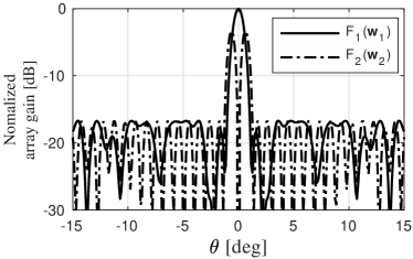
Algorithm 1 with the constant $\epsilon=10^{-5}$ successfully finds a pair of disjoint weight vectors; 53 weights for $F_{1}$ and 67 weights for $F_{2}$ (Figure 3(a)), using the MOSEK solver. The computation time is $6.12$ second. The corresponding beam patterns (Figure 3(c)) meet the specifications we set above. Here, the 3${\rm dB}$ beam width is $0.99^{\circ}$.

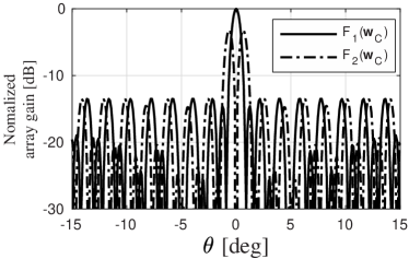
On the other hand, the non-overlapping common weight approaches [10] could not find a feasible solution satisfying the specifications, (even when the mutual coupling matrix is the identity). If we relax the SLL requirements until the remaining beam requirements as well as the initial settings are met, then a solution could be found as shown in Figure 3(b). The corresponding beam patterns have higher SLLs as shown in Figure 3(d). The maximum SLLs of both the sum beam and difference beam are $-13.01{\rm dB}$. However, it must be stressed that our simulation study is limited, and we cannot conclude that the proposed algorithm is superior to the general common weight algorithms [11, 10, 12].

To verify the reliability of the argumentative reselection algorithm, we examine the success rate of finding a feasible solution through Monte Carlo simulation. We count successful runs out of $500$ trials with random initial penalizing vectors $\bf{p}_{1}$, for each SLL from $-16.9{\rm dB}$ to $-16.7{\rm dB}$. As shown in Figure 3(e), the proposed algorithm converges to zero with a $96.2\%$ rate when the SLL is above $-16.78{\rm dB}$.

(a) Normalized magnitudes of weights using the proposed algorithm

(b) Normalized magnitudes of weights using the common shared weight approach (${\bf{w}}_{c}$: common weight vector).

(c) Beam patterns with the weight vectors in (a).

(d) Beam patterns with the weight vectors in (b).

(e) Success rate of finding a feasible solution for different maximum sidelobe levels.

Figure 3: Comparison of the proposed weights and the common weights.

(a) Disjoint antenna distributions of three beams $F_{1}$, $F_{2}$ and $F_{3}$.

(b) Sum beam pattern $F_{1}$.

(c) Difference beam pattern for azimuth $F_{2}$.

(d) Difference beam pattern for elevation $F_{3}$.

(e) Convergence of the cost function $J$ and the number of shared antennas during the iteration.

Figure 4: Two-dimensional monopulse radar beams with disjoint weights.

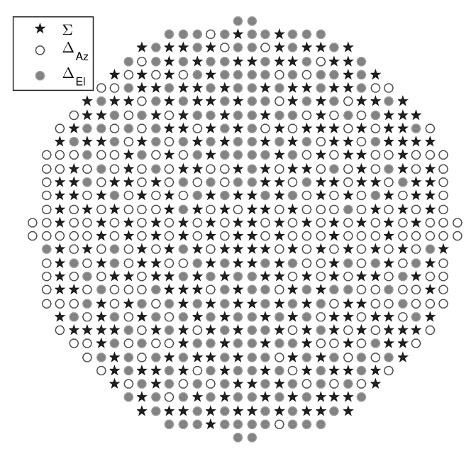
Next, we consider a 2D planar array of 756 antennas with $d=\lambda/2$, which forms three beams; the sum beam $F_{1}$, the azimuth difference beam $F_{2}$ and the elevation difference beam $F_{3}$. We ignore the mutual coupling effect for simple exposition. Our beam specifications for $F_{2}$ and $F_{3}$ will be the same, and therefore, we shall describe $F_{1}$ and $F_{2}$ only. The side-lobe regions for $F_{1}$ and $F_{2}$ are $\Theta_{1}=[5^{\circ},90^{\circ}]\cup[-90^{\circ},-5^{\circ}]$ and $\Theta_{2}=[8^{\circ},90^{\circ}]\cup[-90^{\circ},-8^{\circ}]$, respectively. The maximum SLLs are assumed to be $\tau_{1}=\tau_{2}=-25{\rm dB}$, and the slope $s$, $-22deg^{-1}$.

To speed up the computation of Algorithm 1, we divide the side-lobe regions into two, region a and region b:

$$\Theta_{1a} = [5^{\circ},20^{\circ})\cup(-20^{\circ},-5^{\circ}],$$ (18)

$$\Theta_{1b} = [20^{\circ},90^{\circ}]\cup[-90^{\circ},-20^{\circ}],$$ (19)

$$\Theta_{2a} = [8^{\circ},20^{\circ})\cup(-20^{\circ},-8^{\circ}],$$ (20)

$$\Theta_{2b} = [20^{\circ},90^{\circ}]\cup[-90^{\circ},-20^{\circ}],$$ (21)

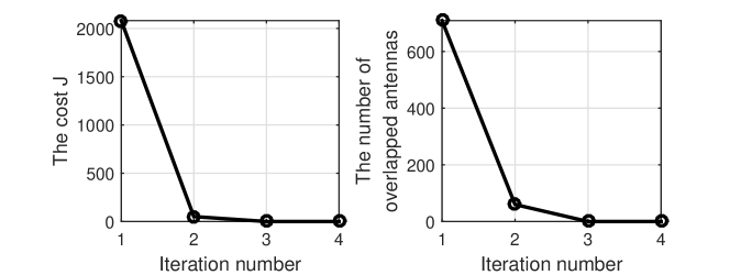
Then we take $10\times 2$ evenly spaced samples each, from $\Theta_{1a}$ and $\Theta_{2a}$, and $35\times 2$ evenly spaced samples each, from $\Theta_{1b}$ and $\Theta_{2b}$. Again Algorithm 1 with $\epsilon=10^{-5}$ finds three disjoint weight vectors; 301 weights for $F_{1}$, 233 weights for $F_{2}$ and 222 weights for $F_{3}$. See Figure 4(a). The computation time is $33.89$ minutes. The corresponding beam patterns, Figure 4(b), (c), and (d) meet the given specifications, and the convergence is shown in Figure 4(e). The $3{\rm dB}$ beamwidth of the sum beam is $4.2^{\circ}$ for both azimuth and elevation angles.

V Concluding Remarks

We have presented the argumentative reselection algorithm which partitions an antenna array into sparse sets, such that the sets of weights are disjoint and give independent desired beam patterns. Sparse subarrays with disjoint weights have a more degree of freedom, and therefore have better control on the beamshapes compared to common (i.e., shared) weight structure. As future work, it may be considered to include the crossing counts of the beamforming network into the objective function to reduce the complexity of the feeder structure.

References

- [1] U. Nickel, “Subarray configurations for digital beamforming with low sidelobes and adaptive interference suppression,” in Proceedings of IEEE International Radar Conference, Alexandria, VA, USA, May 1995, pp. 714–719.
- [2] P. Rocca, L. Manica, R. Azaro, and A. Massa, “A hybrid approach to the synthesis of subarrayed monopulse linear arrays,” IEEE Transactions on Antennas and Propagation, vol. 57, no. 1, pp. 280–283, 2009.
- [3] R. Haupt, “Interleaved thinned linear arrays,” IEEE transactions on antennas and propagation, vol. 53, no. 9, pp. 2858–2864, 2005.
- [4] P. Lopez, J. Rodriguez, F. Ares, and E. Moreno, “Subarray weighting for the difference patterns of monopulse antennas: joint optimization of subarray configurations and weights,” IEEE Transactions on Antennas and Propagation, vol. 49, no. 11, pp. 1606–1608, 2001.
- [5] M. D’Urso, T. Isernia, and E. F. Meliado, “An effective hybrid approach for the optimal synthesis of monopulse antennas,” IEEE transactions on antennas and propagation, vol. 55, no. 4, pp. 1059–1066, 2007.
- [6] L. Manica, P. Rocca, M. Benedetti, and A. Massa, “A fast graph-searching algorithm enabling the efficient synthesis of sub-arrayed planar monopulse antennas,” IEEE Transactions on Antennas and Propagation, vol. 57, no. 3, pp. 652–663, 2009.
- [7] O. M. Bucci, M. D’Urso, and T. Isernia, “Some facts and challegenes in array antenna synthesis problems,” Automatika, vol. 49, no. 1-2, pp. 13–20, 2008.
- [8] S. Caorsi, A. Massa, M. Pastorino, and A. Randazzo, “Optimization of the difference patterns for monopulse antennas by a hybrid real/integer-coded differential evolution method,” IEEE Transactions on Antenna and Propagation, vol. 53, no. 1, pp. 372–376, Jan 2005.
- [9] M. D’Urso and T. Isernia, “Solving some array synthesis problems by means of an effective hybrid approach,” IEEE Transactions on Antenna and Propagation, vol. 55, no. 3, pp. 750–759, Mar 2007.
- [10] S. Kwak, J. Chun, D. Park, Y. Ko, and B. Cho, “Asymmetric sum and difference beam pattern synthesis with a common weight vector,” IEEE Antennas and Wireless Propagation Letters, vol. 15, pp. 1622–1625, 2016.
- [11] A. F. Morabito and P. Rocca, “Optimal synthesis of sum and difference patterns with arbitrary sidelobes subject to common excitations constraints,” IEEE Antennas and Wireless Propagation Letters, vol. 9, pp. 623–626, 2010.
- [12] J. R. Mohammed, “Synthesizing sum and difference patterns with low complexity feeding network by sharing element excitations,” International Journal of Antennas and Propagation, vol. 2017, 2017.
- [13] O. M. Bucci, G. Franceschetti, G. Mazzarella, and G. Panariello, “Intersection approach to array pattern synthesis,” IEE Proceedings, vol. 137, no. 6, pp. 349–356, Dec 1990.
- [14] D. Trincia, L. Marcaccioli, R. Gatti, and R. Sorrentino, “Modified projection method for array pattern synthesis,” in 34th European Microwave Conferencen, 2004, pp. 1379–1400.
- [15] O. M. Bucci, D. Giuseppe, G. Mazzarella, and G. Panariello, “Antenna pattern synthesis: A new general approach,” Proceesings of the IEEE, vol. 82, no. 3, pp. 358–371, Mar 1994.
- [16] Y. Han, C. Wan, W. Sheng, B. Tian, and H. Yang, “Array synthesis using weighted alernating projection and proximal splitting,” IEEE Antenna and Wireless Propagation Letters, vol. 14, pp. 1006–1009, 2015.
- [17] J. Leonardo, A. Quijano, and G. Vecchi, “Alternating adaptive projections in antenna synthesis,” IEEE Transactions on Antenna and Propagation, vol. 58, no. 3, pp. 727–737, Mar 2010.
- [18] I. Ziskind and M. Wax, “Maximum likelihood localization of multiple sources by alternating projection,” IEEE Transactions on acoustics, speech and signal processing, vol. 36, no. 10, pp. 1553–1560, Oct 1988.
- [19] R. Varga, Matrix Iterative Analysis. Englewood Cliffs: Prentice-Hall, 1962.
- [20] T. Isernia, F. Ares Pena, O. M. Bucci, M. D’Urso, J. Gomez, and J. Rodriguez, “A hybrid approach for the optimal synthesis of pencil beams through array antennas,” IEEE Transactions on Antenna and Propagation, vol. 52, no. 11, pp. 2912–2918, Nov 2004.
- [21] J. Quijano and G. Vecchi, “Alternating adaptive projections in antenna synthesis,” IEEE Transactions on Antenna and Propagation, vol. 58, no. 3, pp. 727–737, Mar 2010.
- [22] S. Boyd and L. Vandenberghe, Convex Optimization. Cambridge: Cambridge University Press, 2004, vol. 25.
- [23] B. Friedlander and A. Weiss, “Direction finding in the presence of mutual coupling,” IEEE transactions on antennas and propagation, vol. 39, no. 3, pp. 273–284, 1991.