Key words: Modern Physics, Simulations, MBL.

PACS: 01.30Lb, 01.40R, 01.50H, 01.50J.

Abstract

Modern physics is now a regular course for non-physics majors who do not have to take the accompanying laboratory. This lack of an experimental component puts the engineering students at a disadvantage. A possible solution is the use of computer simulations to add a constructivist element to the class. In this work we present a set of computer simulations of fundamental experiments, key to the teaching of modern physics, as well as their in-class implementation and assessment. Preliminary results indicate that the use of these simulations produce a substantial increase of student comprehension.

1 Introduction

Most universities and colleges offer a regular course on modern physics to non-physics majors. Since in the majority of these cases, a laboratory is not required for this class, this puts engineering students at a disadvantage for understanding key concepts in the foundation of today’s technology. Solving this problem is a complicated issue, as engineering degree plans are already loaded with many courses and labs, and the equipment needed for many modern physics experiments is expensive and difficult to maintain.

This led us to explore different alternatives. Hands on activities have been developed for general physics courses, but not much for modern physics. A big exception is the project CUPS, Consortium for Upper-level Physics Software, which developed a series of computer exercises covering most of the undergraduate physics curriculum, including modern physics¹.

Although the core of the CUPS project provides instructors and students with a tool to teach physics and to develop physical intuition, the exercises lack definite goals, and end up being used mainly as in-class demonstrations and not as part of a constructivist environment. Some accompanying material has been developed to integrate CUPS simulations to student solo activities².

Generally speaking, the purpose of an experimental laboratory is to train the student in relating input variables with output signals, thus identifying physical concepts. If performed under a constructivist environment, the student also learns how to advance hypotheses, develop theories, etc. all under a group format. To have computer simulations helping with all these tasks, the simulations should mimic, as much as possible, a real experiment ³. Some of the problems of making a simulation as real as possible have been discussed in recent publications⁴.

Under this spirit, a project to design, develop, and assess computer versions of key modern physics experiments was initiated with support from the Division of Undergraduate Education of the National Science Foundation (Grant NSF DUE-9651026). This work is a report of the first in-class use and assessment of some of the simulations developed.

2 The simulations

Designing computer simulations as a supplement of a modern physics class imposes a number of limitations. First, to maintain the class structure, the simulations must be planned as one-hour activities to replace a lecture. The topic of each of the simulations has to be strongly correlated with the material covered in class. The simulations must mimic, as much as possible, the setup of the original experiment, including input and output variables. And, to add a constructivist touch, enough degrees of freedom had to be added to the simulations to allow the students to find their own way and to avoid a recipe-like format.

The simulations developed included the classical experiments of Rutherford, Compton, Frank-Hertz, Davisson-Germer, Stern-Gerlack, Zeeman Effect, as well as the determination of Planck’s constant. All simulations have a one-page introduction to the experiment and a two-page activity guide. A typical simulation consists of a full screen with controls and output devices. As an illustration, fig. 1 shows the control panel for the simulation of the Frank-Hertz experiment.

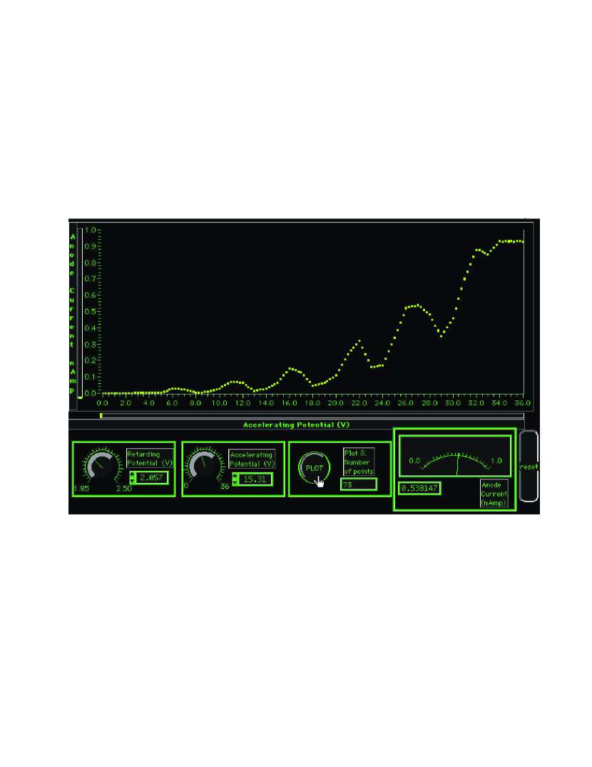
Figure 1: Control panel for the simulation of the Frank-Hertz experiment.

Along with the description of the experiment and activity guide, assessment instruments were developed for each of the simulations. Pre- and post- examinations were designed to measure the impact of the simulation taken.

The first application of the simulations to modern physics students took place in the Fall of 1997 and Spring of 1998 at the University of Texas at El Paso (UTEP), and at the University of Wisconsin-Oshkosh (UWO). In the following sections, as a case study, we describe one of the simulations in detail, and present assessment results of the use of several of these simulations.

3 A study case: Davisson-Germer

Davisson and Germer performed hundreds of experiments to demonstrate the wave-like properties of electrons scattering off a nickel crystal ^5-7. The electrons constituting an incident beam were thermally emitted from a tungsten ribbon and projected normally to a perfectly clean, gas-free, Ni target. The intensity of scattering of this homogeneous beam of incident electrons was detected by movable detector in the range of colatitude angles from 0 to 90 degrees. For a fixed voltage, maximum intensity peak appeared only at a certain colatitude angle.

Wavelengths associated with electrons using the De Broglie’s relation $\lambda~{}=~{}h~{}/~{}m_{e}~{}v_{e}$ (with $h$ being Planck’s constant, $m_{e}$ the electron mass and $v_{e}$ the experimentally set value for velocity) perfectly coincided, in a certain range of electrons’ kinetic energies, with the wavelength values obtained by using Bragg’s formula for maximum diffraction intensity $d\sin\theta=n\lambda$, where $\theta$ is the angle where maximum intensity is observed, $d$ is the interatomic spacing, and $n$ is the order of the diffraction maximum. Later on, experiments with different particles were performed and similar results were obtained. The general conclusion was that particles behave like waves.

3.1 Description of the simulation

The simulation was designed to reproduce the experiment using a black-box approach. Input and output variables, such as voltages, type of particles, etc. were identified, and relationships among them were included as the inner side of the black-box.

For the Davisson-Germer experiment, the input variables are the accelerating voltage, the type of particles (electrons), the diffracting crystal, and the detection angle. Most of these variables can be changed by the user. The only output variable is the scattering intensity which varies according to all input variables.

In the computer program, the connection between the final intensity and the input variables comes from fitting original data, and not from a real- time simulation. The data for the simulation was digitized from the original articles of Davisson and Germer ^5-7 using experimentally obtained curves for seven different values of voltages from the range of 40 to 68 Volts and for angles between 0 and 90 degrees. Interpolation between any two curves makes possible to cover a larger range of voltages and colatitude angles. In this way, the students have the same degrees of freedom that the original researchers had. On their own, students must realize that to obtain meaningful results, an specific voltage must be fixed first, and that the detection angle must be varied many times.

3.2 Assessment and data collection

The assessment of the activity was designed to test the student’s knowledge of the experiment before and after using the simulation. Again, taking the experiment as a black-box, elements of the experiment were identified to be included in the pre- and post-tests. The assessment exams and the simulation were taken by the students after covering the material in class. Two UTEP modern physics classes totalling over 50 students participated in this study. Due to the relatively small number of students, the possibility of using a control group was discarded.

The pre- and post-exams for the Davisson-Germer simulation are shown in figs. 2 and 3. Most of the questions refer to basic knowledge of the physical ingredients of the experiment, and not to the meaning of the physical concepts.

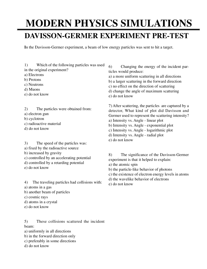
Figure 2: Pre-exam for the simulation of the Davisson-Germer experiment.

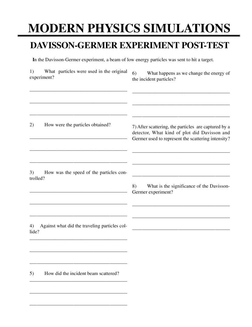
Figure 3: Post-exam for the simulation of the Davisson-Germer experiment.

The pre-test was administered in 10 minutes. Afterwards the students were given the activity guide which consisted of a series of steps to illustrate the use of the simulation, and a series of open-ended questions to guide the students. Working in groups of two, three or four, the students completed the simulation in about 45 minutes, and immediately after running the simulation the students completed the post-test in about 10 more minutes.

As seen in figs. 2 and 3, the pre- and post-examinations are much alike, except for the format. This was to facilitate the correlation between exams on a question-to-question basis. The grading of the essay-type post-exam took into account the depth of knowledge shown in the answers⁸.

3.3 Results

For the case of the Davisson-Germer experiment, the results regarding the student performance in the pre- and post-exams are displayed in figs. 4. The same information, in terms of the questions, is shown in fig. 5.

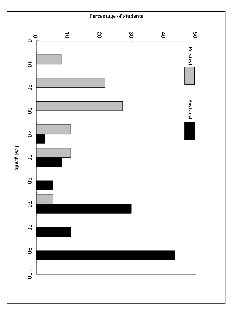
Figure 4: Student performance in the pre- and post-exams.

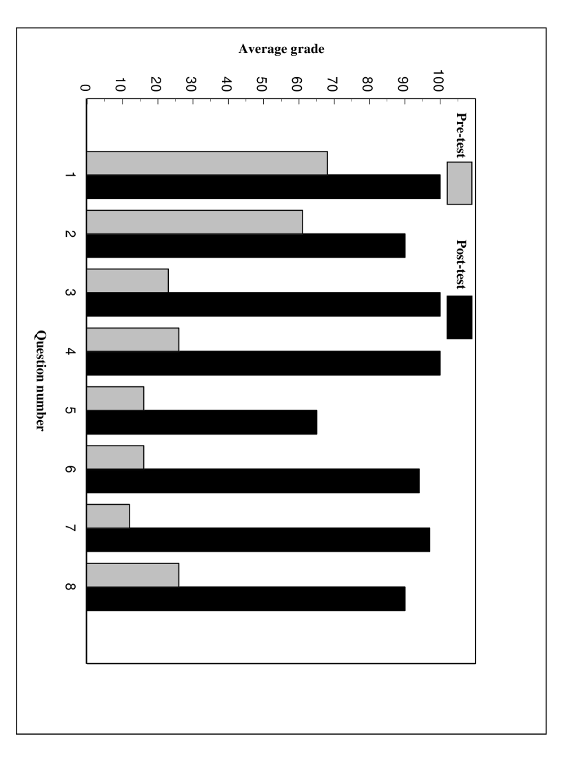
Figure 5: Student performance per questions in the pre- and post-exams.

4 Results from other simulations

Altogether, four simulations were used and tested with the UTEP students, and one with one UWO modern physics class. The simulations used at UTEP were the Rutherford, Compton, Frank-Hertz, and Davisson-Germer, and the one tested at UWO was the Frank-Hertz.

Assessment analyses similar to the one described before were performed for all the experiments. Results for the pre- and post-exams are presented in fig. 6. As before, the gain from the pre- to the post exams varied from 30% to 50%, much larger than the canonical $10$ to $20$% generally obtained with traditional teaching methods, and on the higher end of the percentages obtained with interactive engagement methods in introductory physics courses⁹.

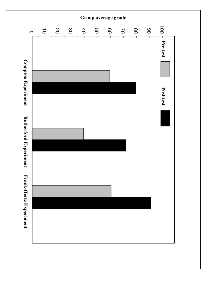
Figure 6: Results for the pre- and post-exams performed for all the experiments.

As an informal assessment, we collected anecdotal information from students, professors, and experts on the field. Common student comments were:

• “The labs were useful and successful”

• “The laboratories offered in the physics department were very useful to me. They gave me a more in-depth knowledge regarding the subject”

• “The class lecture gave me a good view behind the experiments, but the possibility of changing parameters and seeing the process of the experiment itself, gave me more details and helped me understand the material much better”

• “I feel more knowledgeable of the material for which I had the chance to run the experiments than those just presented in class. Also, it encouraged team discussion, and more ideas were brought up and shared among the group members”.

5 Conclusions and further directions

To add an interactive element to modern physics courses, we designed, developed, and assessed computer versions of several key modern physics experiments. Using the simulations as part of the class, students were tested before and after the use of the simulation. We presented, as a study-case, the simulation, and the pre- and post-exams for the Davisson-Germer experiment. Results for other simulations tested at UTEP and at UWO were also presented.

In conclusion, the use of the simulations appears to be very benefitial for the students. Aside from extremely positive feedback from the participant instructors and students, the pre- and post-exams showed a significant increase in the understanding of the basic physics ingredients of the experiments.

6 Acknowledgement

This work was partially supported by the National Science Foundation under grant NSF DUE-9651026, and UTEP’s NSF-MIE program. We thank Dr. R. Fitzgerald, G. Vandergrift, from UTEP, and Dr. C. Passow, from UWO, for allowing us to test the simulations in their modern physics classes. We acknowledge interesting discussions with Dr. R. Donangelo, from Universidad Federal do Rio de Janeiro, and Drs. Pat Heller and Ken Heller, from the University of Minnesota. We also thank students J. Correa and M. Cortés for helping with the programming and assessment of some of the simulations.

List of figures

• Control panel for the Frank-Hertz experiment.

• Davisson-Germer pre-test.

• Davisson-Germer post-test.

• Grade distributions for the pre- and post-tests of the Davisson-Germer simulation.

• Average grade distribution for the pre- and post-tests per question of the Davisson-Germer simulation.

• Group average grade distributions for the pre- and post-tests for other simulations.

References

- [1] D. Brandt, J.R. Hiller and M.J. Moloney, Modern Physics Simulations, Consortium for Upper-level Physics Software, (John Wiley and Sons, New York, 1995).
- [2] R. Ehrlick, M. Dworzecka, W. MacDonald, and J. Tuszynski, Computers in Physics Education 7, 508 (1993).
- [3] B. Hasson and A. Bug, The Physics Teacher 33, 230 (1995).
- [4] E.L. Lewis, J.L. Stern, M.C. Linn, Educational Technology 45, (Jan. 1993).
- [5] C. Davisson and L.H. Germer, The Physical Review 30, 705 (1927).
- [6] C. Davisson and L.H. Germer, Physics 14, 317 (1928).
- [7] C. Davisson and L.H. Germer, Physics 14, 619 (1928).
- [8] K. Worth, C. Matsumoto, J.O. Sandler, Insights: Lifting Heavy Things, (Education Development Center, Newton, Massachusets, 1994), p. 25.
- [9] R.R. Hake, American Journal of Physics 66, 64 (1998).