Efficient Structured Pruning and Architecture Searching for Group Convolution

Abstract

Efficient inference of Convolutional Neural Networks is a thriving topic recently. It is desirable to achieve the maximal test accuracy under given inference budget constraints when deploying a pre-trained model. Network pruning is a commonly used technique while it may produce irregular sparse models that can hardly gain actual speed-up. Group convolution is a promising pruning target due to its regular structure; however, incorporating such structure into the pruning procedure is challenging. It is because structural constraints are hard to describe and can make pruning intractable to solve. The need for configuring group convolution architecture, i.e., the number of groups, that maximises test accuracy also increases difficulty.

This paper presents an efficient method to address this challenge. We formulate group convolution pruning as finding the optimal channel permutation to impose structural constraints and solve it efficiently by heuristics. We also apply local search to exploring group configuration based on estimated pruning cost to maximise test accuracy. Compared to prior work, results show that our method produces competitive group convolution models for various tasks within a shorter pruning period and enables rapid group configuration exploration subject to inference budget constraints.

1 Introduction

Convolutional Neural Networks (CNNs) are being deployed on devices ranging from large servers to small edge systems that have various computing capability. While deploying pre-trained CNN models, we intend to maximise their test accuracy under inference budget constraints, e.g., maximum numbers of parameters and operations. Pruning is a workable solution that removes parameters contributing little to test accuracy, and its success has been demonstrated in numerous prior works [6, 5, 29, 24]. However, many pruned models can hardly achieve practical test-time speed-up due to irregular sparsity, which results in imbalanced workloads that only customised GPU kernels or specialised hardware [5] can handle. Therefore, we are motivated to prune pre-trained models into compact, accurate, and regular sparse models.

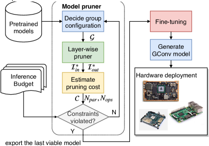
Figure 1: The overall work-flow. Symbols are explained in Section 3.

Group convolution (GConv) [17, 44, 15] is a promising pruning target. A GConv layer consists of multiple identically configured convolution layers, which as a whole can be considered as a regular sparse convolution layer with equivalent sparsity across its channels. GConv also has good learning capability as presented in [44, 15, 49]. Given these potential benefits, we expect that pruning pre-trained CNNs into GConv-based models can improve test-time performance regarding speed and accuracy.

However, pruning into GConv is a challenging structured pruning problem, i.e., pruned parameters should follow patterns of their positions on input and output channel axes. These structural constraints turn pruning into a hard-to-solve combinatorial optimisation problem. Meanwhile, the number of groups should be determined for all layers, which is not a trivial procedure as well. These two problems have not been properly resolved by prior works [50, 32, 12] yet: they may require training from scratch, manually determining group configuration, or adding overhead during inference. There is still room for improvement.

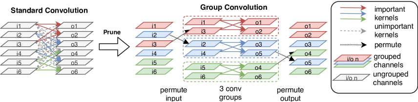
Figure 2: An overview of our pruning objective. The convolution layer has 6 input and output channels and we intend to prune it into a group convolution with 3 groups. Our method will figure out which channels should belong to which groups. The measurement of kernel importance is explained in Section 3.

This paper presents a novel GConv pruning method that addresses both challenges. For the structured pruning problem, we formulate it as finding the optimal channel permutation that implicitly imposes the structural constraints of GConv and solve it rapidly through heuristics. This solution is named as layer-wise pruner (Section 3.2). To determine the number of groups for each layer, we employ the layer-wise pruner to estimate the cost of pruning with different given numbers of groups, and apply local search to explore feasible solutions within limited time. This part is introduced as model pruner (Section 3.3). Finally, we prune the model by the best sparsity configuration that has been explored. We follow the spirit in [25] to either fine-tune the pruned model or train from scratch the topology. Empirically compared to prior papers, our method produces GConv models that run efficiently in test-time, requires shorter pruning period, and further allows the exploration of sparsity configurations subject to inference budget constraints (Section 4). Our code-base is publicly available.

2 Background and Related Work

Group Convolution.

A GConv layer works by partitioning its input channels into disjoint groups and separately convolving each with a group-specific set of filters. Concretely, given an input tensor shaped $(C_{\text{in}},H,W)$, we run $G$ convolution layers between each pair of $(C_{\text{in}}/G,H,W)$ input partition and $(C_{\text{out}}/G,C_{\text{in}}/G,K_{\text{h}},K_{\text{w}})$ weight group. $G$ denotes the number of groups and indicates the sparsity of the GConv layer. A GConv is sparser when $G$ is larger. $C_{\text{out}}$ is the number of output channels and $(K_{\text{h}},K_{\text{w}})$ is the kernel shape. Output from these convolution layers are concatenated along the channel axis to produce the final result.

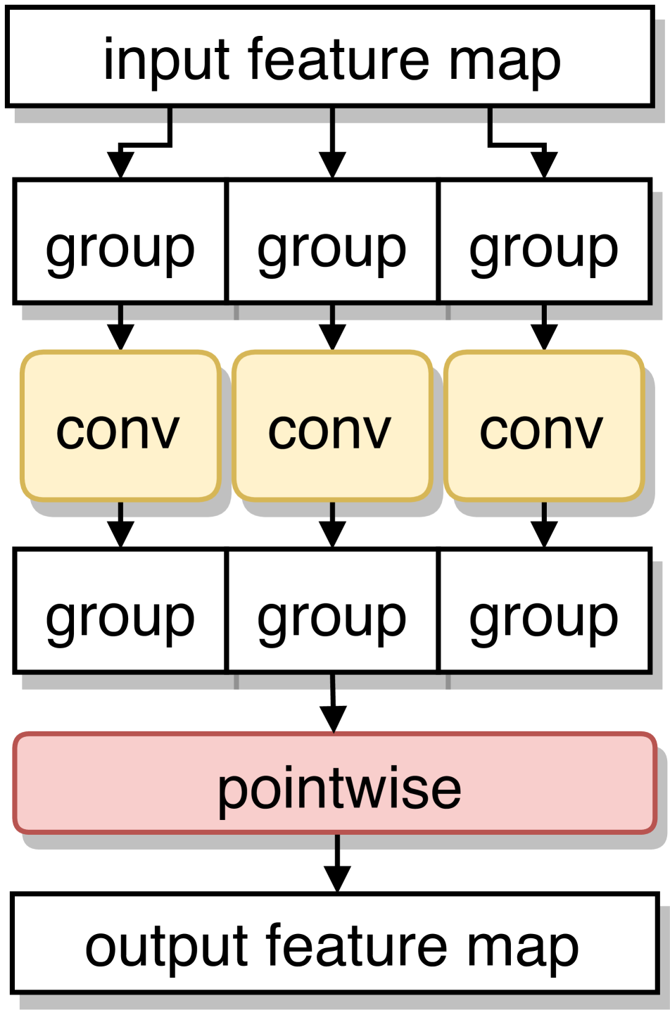
(a) Pointwise-based

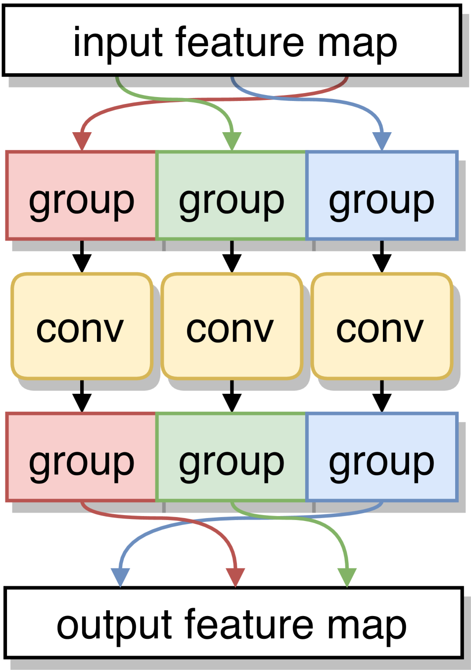
(b) Permutation-based

Figure 3: Two variants of GConv that are different in information exchange mechanism.

To improve the learning capacity, we need to encourage information exchange among groups [49]. [44, 15, 32] suggest using pointwise convolution, which applies $1\times 1$ kernels to correlate channels (Figure 3(a)). It is versatile while it can incur unbearable overhead: $C_{\text{in}}C_{\text{out}}$ additional parameters and $C_{\text{in}}C_{\text{out}}HW$ more FMA operations are required. Additionally, it cannot deal with $1\times 1$ group convolution, which is critical since recent efficient CNN heavily rely on them [10, 36, 49]. [50] applies block Hadamard transform, which is more efficient but still requires extra computation. On the other hand, permuting channels is a much simpler way to mingle groups (Figure 3(b)) since neither additional FMA nor parameter is required. [49, 48, 43] permute by interleaving channels from different groups, which is also called channel shuffle. We apply permutation as well for its efficiency and the optimisation purpose (Section 3).

To construct a CNN by GConv, one can build and train from scratch [49, 15, 44, 50, 42], or prune from pre-trained models. CondenseNet [12] prunes by a multi-stage, from-scratch training and regularisation procedure. FLGC [39] follows a similar approach to optimise the GConv topology while training from scratch. Peng et al. [32] consider a GConv layer as a low-rank approximation of a convolution layer. This approach produces models with high test accuracy but always needs to add pointwise layers.

Network Pruning.

Our method can be regarded as structural, sensitivity-based network pruning. Sensitivity pruning selects weights that contribute little to test accuracy and removes them directly based on specific criteria, including: magnitude, e.g., L1, L2 norms [27, 5, 20, 26], first-order [29, 3] or second-order [19, 7, 2] gradients, average percentage of zero [26, 11], singular values [32, 28]. [46] considers the importance as a global score. Each criterion has different computation efficiency and measurement accuracy on contribution from weights.

Alternatively, there are regularisation based methods that sparsify models through curated regularisers so that models can have enough time to adapt. L1 norm is studied for sparsifying CNN models in [24, 5], and it normally produces unstructured, irregular models. Some other methods use group LASSO [47] to encode specific structures during regularisation, such as channel or filter level pruning [30, 40, 18]. Specifically, CondenseNet [12] adapts this method to GConv pruning. Pruning by LASSO regularisers is more difficult due to non-differentiability around optimal points and hyperparameters are hard to tune.

Neural Architecture Search (NAS).

NAS is a recently developed technique that enables automatic exploration of neural network architectures under specific constraints. The core mechanism behind is normally the REINFORCE algorithm [41], specifically, [51, 52, 37, 38] consider searching architectures under different platform constraints. Evolutionary algorithm is another option [33, 1, 22]. To make NAS more efficient, using gradient-based method [23] or reducing the search space [21] is proposed as well. Parts of our method overlap the objective of NAS: we intend to search for the group configuration under inference budget. This is a novel objective and we provide an efficient solution based on our pruning method, and we are intrigued to see how mainstream NAS algorithms can be applied to this research question.

3 Method

Our objective is to prune a pre-trained CNN model into a GConv based model (Figure 2). The following sections formulate GConv pruning as an optimisation problem that searches for channel permutations, demonstrate the layer-wise heuristic pruning algorithm that efficiently solves this problem, and show how to explore model sparsity under inference budget constraints.

3.1 Group Convolution Pruning

$$\tilde{\textbf{{X}}}_{c}=\textbf{{X}}_{\mathcal{I}_{\text{in}}(c)}\quad\tilde{\textbf{{Y}}}^{g}=\textbf{{W}}^{g}*\tilde{\textbf{{X}}}^{g}\quad\textbf{{Y}}_{f}=\tilde{\textbf{{Y}}}_{\mathcal{I}_{\text{out}}(f)}$$ (1)

$$\forall\ 1\leq f\leq C_{\text{out}}\quad 1\leq c\leq C_{\text{in}}\quad 1\leq g\leq G$$

Group convolution.

We can formulate GConv by mapping from Figure 3(b) to (1). X and Y are both 3D tensors indicating input and output feature maps; $\textbf{{X}}_{c}$ and $\textbf{{Y}}_{f}$ are 2D images belong to input channel $c$ and output channel $f$ respectively; and $\textbf{{W}}\in\mathbb{R}^{C_{\text{out}}\times C_{\text{in}}\times K_{\text{h}}\times K_{\text{w}}}$ is a 4D tensor denoting weights. $\mathcal{I}_{\text{in}}$ and $\mathcal{I}_{\text{out}}$ are two sets of channel indices that specify permutation, e.g., $\mathcal{I}_{\text{in}}(c)$ is permuted to $c$. When performing GConv, we permute X into $\tilde{\textbf{{X}}}$ by input channel indices $\mathcal{I}_{\text{in}}$, partition $\tilde{\textbf{{X}}}$ into $G$ groups $\{\tilde{\textbf{{X}}}^{g}\in\mathbb{R}^{C_{\text{in}}/G\times H\times W}\}_{g=1}^{G}$ along channel, run a convolution layer ($*$) between $\textbf{{X}}^{g}$ and weight group $\textbf{{W}}^{g}\in\mathbb{R}^{C_{\text{out}}/G\times C_{\text{in}}/G\times K_{\text{h}}\times K_{\text{w}}}$ for each group $g$, concatenate their output $\{\tilde{\textbf{{Y}}}^{g}\}_{g=1}^{G}$ into a tensor $\tilde{\textbf{{Y}}}$ by channel, and permute $\tilde{\textbf{{Y}}}$ by output channel indices $\mathcal{I}_{\text{out}}$ to produce the result Y.

Alternatively, we can treat GConv as a sparse convolution. To illustrate this idea, we reshape W into a 6D tensor $\mathcal{W}\in\mathbb{R}^{G\times G\times C_{\text{out}}/G\times C_{\text{in}}/G\times K_{\text{h}}\times K_{\text{w}}}$ by partitioning the input and output channels of W into $G$ groups. Considering each $K_{\text{h}}\times K_{\text{w}}$ kernel as a single element, this representation can be viewed as a generalised block matrix with $G\times G$ number of $C_{\text{out}}/G\times C_{\text{in}}/G$ sized blocks. Similarly, we can partition X and Y into 4D tensors $\mathcal{X}\in\mathbb{R}^{G\times C_{\text{in}}/G\times H\times W}$ and $\mathcal{Y}\in\mathbb{R}^{G\times C_{\text{out}}/G\times H\times W}$ and view them as generalised block vectors. Note that 2D images are considered as elements in these block matrices.

$$\mathcal{Y}_{g_{f}}=\sum_{g_{c}=1}^{G}\mathcal{W}_{g_{f}g_{c}}*\mathcal{X}_{g_{c}}\quad\forall\ 1\leq g_{f}\leq G$$ (2)

$$\begin{aligned} \mathcal{Y}&=\operatorname*{\mathsf{diag}}(\{\mathcal{W}_{gg}\}_{g=1}^{G})*\mathcal{X}\\ &=\begin{bmatrix}\mathcal{W}_{11}&0&\cdots&0\\ 0&\mathcal{W}_{22}&\cdots&0\\ \vdots&\vdots&\ddots&\vdots\\ 0&0&\cdots&\mathcal{W}_{GG}\end{bmatrix}\begin{bmatrix}\mathcal{X}_{1}\\ \mathcal{X}_{2}\\ \vdots\\ \mathcal{X}_{G}\\ \end{bmatrix}=\begin{bmatrix}\mathcal{X}_{1}*\mathcal{W}_{11}\\ \mathcal{X}_{2}*\mathcal{W}_{22}\\ \vdots\\ \mathcal{X}_{G}*\mathcal{W}_{GG}\\ \end{bmatrix}\end{aligned}$$ (3)

We can define convolution among group partitioned tensors $\mathcal{Y}=\mathcal{W}*\mathcal{X}$ as a generalised block matrix-vector multiplication. Here, the multiplication between entries in $\mathcal{W}$ and $\mathcal{X}$ is interpreted as convolution. For example, (2) illustrates the dot-product routine that computes the convolution between two blocks in $\mathcal{W}$ and $\mathcal{X}$. Interestingly, if $\mathcal{W}$ is a generalised block-diagonal matrix, i.e, only $\mathcal{W}_{gg}$ are non-zero, then this convolution becomes a group convolution (3). Ignoring permutations in (1) and considering $\mathcal{W}_{gg}$ as $\textbf{{W}}^{g}$, $\mathcal{X}_{g}$ as $\textbf{{X}}^{g}$, and $\mathcal{Y}_{g}$ as $\textbf{{Y}}^{g}$, it is obvious that (1) is equivalent to (3). This is the basis of the following analysis.

$$\begin{bmatrix}w_{11}&w_{12}&w_{13}\\ w_{21}&w_{22}&w_{23}\\ w_{31}&w_{32}&w_{33}\end{bmatrix}\xrightarrow[\mathcal{I}_{\text{in}}=\{1,3,2\}]{\mathcal{I}_{\text{out}}=\{2,1,3\}}\begin{bmatrix}w_{21}&w_{23}&w_{22}\\ w_{11}&w_{13}&w_{12}\\ w_{31}&w_{33}&w_{32}\end{bmatrix}$$ (4)

Pruning and channel permutation.

Pruning means removing weights unimportant to model accuracy from a trained model based on a specific criterion. (3) shows that removing weights to form a block-diagonal matrix is equivalent to pruning into GConv. A straightforward approach to prune is just removing kernels outside the diagonal. It can hardly perform well since we cannot guarantee that kernels around the diagonal are important to the model accuracy. Since we allow channel permutation on both input and output, we can formulate pruning as an optimisation problem that targets at finding the channel permutation that can move most of the important kernels to diagonal blocks. To be specific on permutation, (4) shows an example result after applying a pair of permutation indices $\mathcal{I}_{\text{out}}$ and $\mathcal{I}_{\text{in}}$ on weights. $w_{ij}$ denotes a single kernel, and rows and columns represent output and input channel axes respectively.

Optimisation problem.

(5) formulates the optimisation problem of finding optimal permutations $\mathcal{I}_{\text{in}}^{*}$ and $\mathcal{I}_{\text{out}}^{*}$. We need to find the pair of permutations such that, after applying it on the original weights W, the importance reduction caused after removing weights outside the diagonal will be minimal. $\{\tilde{\mathcal{W}}_{gg}\}_{g=1}^{G}$ denotes all the diagonal-blocks of permuted weights. $\mathcal{C}$ is the criterion that measures the importance (Section 2). We choose a magnitude-base criterion that sums the L2 norm of all kernels, based on the assumption that kernels with greater magnitude contribute more to model accuracy.

$$\operatorname*{arg\,min}_{\mathcal{I}_{\text{in}}^{*},\mathcal{I}_{\text{out}}^{*}} \quad\mathcal{C}(\textbf{{W}})-\mathcal{C}\left(\operatorname*{\mathsf{diag}}(\{\tilde{\mathcal{W}}_{gg}\}_{g=1}^{G})\right)$$ (5)

$$\mathbf{s.t.} \quad\tilde{\mathcal{W}}_{g_{f}g_{c}}\equiv\tilde{\textbf{{W}}}^{g_{f}g_{c}}\quad\tilde{\textbf{{W}}}_{fc}=\textbf{{W}}_{\mathcal{I}_{\text{out}}^{*}(f)\mathcal{I}_{\text{in}}^{*}(c)}$$

We notice that solving this problem requires similar efforts as solving the Bottleneck Travelling Salesman Problem (BTSP) [4], which is known to be NP-complete. Since the number of channels can be hundreds or even thousands, directly solving this problem is computationally intractable. Next section presents a heuristic algorithm that produces satisfiable solutions within a limited time.

3.2 Prune a Layer

This section focuses on the layer-wise pruning problem: for a given sparsity, indicated by the number of groups $G$, we aim to find the pair of column-wise and row-wise permutations that minimise the pruning objective defined in (5). Column and row refer to input and output channel axes of weights respectively.

$$\max_{\mathcal{I}_{\text{out}},\mathcal{I}_{\text{in}}}\quad\sum_{g=1}^{G}\sum_{f=1}^{\nicefrac{{C_{\text{out}}}}{{G}}}\sum_{c=1}^{\nicefrac{{C_{\text{in}}}}{{G}}}\left\lVert\tilde{\mathcal{W}}_{ggfc}\right\rVert$$ (6)

We start from replacing $\mathcal{C}$ with L2 norm to convert the original problem to an equivalent maximisation problem that maximises the sum of L2 norm of weight kernels in diagonal blocks of $\tilde{\mathcal{W}}$, as shown in (6).

$$\sigma_{\mathrm{c}}(c,g) =\sum\nolimits_{f=\frac{g-1}{G}C_{\text{out}}+1}^{\frac{g}{G}C_{\text{out}}}\left\lVert\textbf{{W}}_{fc}\right\rVert$$ (7)

$$\sigma_{\mathrm{f}}(f,g) =\sum\nolimits_{c=\frac{g-1}{G}C_{\text{in}}+1}^{\frac{g}{G}C_{\text{in}}}\left\lVert\textbf{{W}}_{fc}\right\rVert$$

Sub-problem.

Suppose we only maximise the sum-of-norm for the $G$-th block diagonal component $\mathcal{W}_{G,G}$, and we are only allowed to permute input channels, an intuitive solution for this sub-problem is sorting input channels by $\sigma_{\mathrm{c}}(c,G)$ (7). Under the given restrictions, sorting by $\sigma_{\mathrm{c}}$ in an increasing order practically moves the most important weights to $\mathcal{W}_{GG}$. Similarly, if only output channels are permitted to permute, we can sort them by $\sigma_{\mathrm{f}}(f,G)$ as well to maximise the importance of $\mathcal{W}_{GG}$.

Heuristic Algorithm.

This intuition leads us to a heuristic algorithm that solves (6). Instead of considering this problem as a whole, we dissect it into sub-problems similar to the example above, which can be solved block by block through sorting with regards to $\sigma_{\mathrm{c}}$ and $\sigma_{\mathrm{f}}$. Specifically:

1. Our algorithm runs in $G$ iterations and the $g$-th iteration works on optimising block $\mathcal{W}_{G-g+1,G-g+1}$ only.

2. Each iteration sorts input and output channels by $\sigma_{\mathrm{c}}(c,g)$ and $\sigma_{\mathrm{f}}(f,g)$ respectively for $N_{S}$ rounds.

3. All channels related to previously resolved blocks remain frozen, i.e., the upper bounds for $f$ and $c$ that can be sorted are $(G-g+1)C_{\text{out}}/G$ and $(G-g+1)C_{\text{in}}/G$.

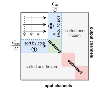
Figure 4: This figure shows $\mathcal{W}$ that is being sorted. It is running at the 3rd block (green). Kernels covered by previous blocks (red) are now frozen for further sorting (gray). When updating the 3rd block, input channels (columns) are sorted by $\sigma_{\mathrm{c}}(c,3)$ in range ① and output channels (rows) are sorted by $\sigma_{\mathrm{f}}(f,3)$ in range ②.

Figure 4 illustrates an intermediate step of this algorithm. $N_{S}$ is a hyperparameter that denotes the number of sorting rounds for each block. A sorting round means sorting input channels and then output channels. $N_{S}$ is necessary since we permit sorting both input and output channels: after finishing a sorting round, the increasing order of input channels regarding $\sigma_{\mathrm{c}}$ may be violated, and running a new round may fix it. For example, as shown in Figure 4, kernels in the white region are not covered in $\sigma_{\mathrm{c}}$ when sorting input channels at first, and after output channels are sorted, some may enter the blue region and affect the evaluation of $\sigma_{\mathrm{c}}$. What we present here is a polynomial time algorithm and its complexity is $\mathcal{O}(GN_{S}\times(\frac{C_{\text{in}}}{G}\log(\frac{C_{\text{in}}}{G})+\frac{C_{\text{out}}}{G}\log(\frac{C_{\text{out}}}{G})))$.

$$\text{recovery ratio}=\frac{\sum_{g,f,c}\left\lVert\tilde{\mathcal{W}}_{ggfc}^{*}\right\rVert}{\sum_{g,f,c}\left\lVert\mathcal{W}_{ggfc}\right\rVert}$$ (8)

Empirical Evaluation.

We empirically justify this algorithm by running it on randomly generate sample weights and real-world pre-trained models. We first create a block-diagonal matrix, then permute it by random indices, and try to recover the original permutation as much as possible. We measure the quality by the recovery ratio defined by (8), in which $\tilde{\mathcal{W}}^{*}$ denotes weights permuted by optimal permutations decided by our algorithm. We notice that the recovery ratio becomes higher for more samples when $N_{S}$ increases, and when $N_{S}=10$, most samples can achieve 100% recovery ratio. It shows that by using our heuristic algorithm with $N_{S}=10$ we can move most important weights to diagonal blocks, which implicitly guarantees our GConv pruning performance since we remove weights out of diagonal blocks.

We also measure the recovery ratio on weights from pre-trained ResNet-50: as shown on the right of Figure 5, compared with the baseline that does no sorting ($N_{S}=0$), our method can recover about 3% more for different numbers of groups. Besides the recovery ratio, we compare the final test accuracy between using and not using our heuristic method in Table 3. In the future, we will provide formal proof regarding the performance of this heuristic algorithm.

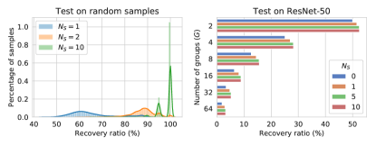
Figure 5: Evaluation results on the heuristic algorithm. Recovery ratio is the percentage of magnitude, measured by L2 norm, retained in the diagonal blocks after pruning.

Table 1: Evaluation on CIFAR-10 (C10) and CIFAR-100 (C100). Number of parameters (# Param.) and operations (# FLOPS) are measured on CIFAR-100. Note that we consider one FMA as two operations. The DenseNet-86 on the last line is named as CondenseNet-86 in its original paper [12].

	Test Error (%)
Model	C10	C100	# Param.	Pruned	# FLOPS	Pruned
ResNet-164 (Baseline)	4.81	22.83	1.73M	—	504M	—
ResNet-164 (40% pruned)	4.91	22.71	1.46M	15.5%	462M	8.4%
ResNet-164 (60% pruned)	5.08	23.66	1.21M	29.7%	430M	14.7%
ResNet-164 (40% pruned) [24]	5.08	22.87	1.46M	15.5%	333M	33.3%
ResNet-164 (60% pruned) [24]	5.27	23.91	1.21M	29.7%	247M	50.6%
DenseNet-86 (Baseline) [12]	4.44	20.57	2.03M	—	506.1M	—
DenseNet-86 ($G=4$)	5.94	25.96	0.59M	70.94%	132.7M	73.77%
DenseNet-86 (opt. for 50% budget)	4.98	22.41	1.00M	50.74%	256.5M	49.33%
CondenseNet-86 ($G=4$) [12]	5.00	23.64	0.59M	70.94%	132.7M	73.77%

3.3 Optimise Group Configuration

To prune a whole CNN model into one that uses GConv, we need to determine the group configuration, which is a combination of all layers’ numbers of groups. Group configuration can affect both the model accuracy and the inference budget, and therefore, finding an optimal group configuration is an optimisation problem that maximises accuracy under budget constraints. Prior papers use some ad-hoc rules to decide group configuration, e.g., using a uniform group number for all layers [12] or scaling the number of groups by the number of channels [32, 50]. When using these methods, the only way to find the configuration that gives the highest model accuracy is by trial-and-error, i.e., manually picking a group configuration and fine-tuning from it, which is cumbersome. To address this problem, we propose a group configuration optimisation algorithm, which finds near-optimal configuration regarding model accuracy by utilising pre-trained weights through our GConv pruning algorithm.

$$\operatorname*{arg\,min}_{\mathcal{G}} \ \sum_{l=1}^{L}\mathsf{cost}(\mathcal{W}^{(l)},\mathcal{G}_{l})$$ (9)

$$\mathbf{s.t.} \ \sum_{l=1}^{L}\frac{N_{\text{par}}^{(l)}}{\mathcal{G}_{l}}\leq N_{\text{par}}^{\text{max}}\quad\sum_{l=1}^{L}\frac{N_{\text{ops}}^{(l)}}{\mathcal{G}_{l}}\leq N_{\text{ops}}^{\text{max}}$$

This method is formulated as (9). The variable $\mathcal{G}$ is a vector that specifies the number of groups of each layer $l$. The function $\mathsf{cost}$ denotes the minimal pruning cost returned from solving (5). We assume that the lower the pruning cost, the higher the accuracy of a pruned model. The objective is to minimise the sum of estimated pruning cost of all layers subject to constraints on the maximum numbers of parameters $N_{\text{par}}^{\text{max}}$ and operations $N_{\text{ops}}^{\text{max}}$.

Our approach is a local search algorithm [35]. We notice that by adding the number of groups of a layer, the total cost increases and the numbers of parameters and operations decrease. Based on this observation, we devise this local search algorithm by starting with a $\mathcal{G}$ that sets $G$ to 1 for all layers, and in each of the following iterations, selecting one layer that minimally increases the cost when its number of groups is changed to the nearest larger candidate. The whole procedure terminates when the resource constraints are satisfied. To estimate pruning cost more precisely, we can optionally prune and fine-tune the model by the current $\mathcal{G}$ at the end of each iteration. This algorithm is summarised in Algorithm 1.

1 $\mathcal{G}\leftarrow\text{maximal numbers of groups of all layers}$;

2 while $\text{budget of }\mathcal{G}\text{ is under constraints}$ do

3       $i\leftarrow\text{layer that reduces cost the most}$;

4       $\mathcal{G}(i)\leftarrow\text{next larger number of groups for }i$;

5       (optional) prune model by $\mathcal{G}$ and then fine tune;

6      

7return $\mathcal{G}$;

Algorithm 1 The local search algorithm to solve (9)

As a final step, based on the optimised $\mathcal{G}$, we prune and fine-tune the given model again to improve its model accuracy as much as possible. Empirically we find this algorithm works well. As shown in the next section (Figure 6), we can explore configurations within given budget and the explored models perform competitively compared to ad-hoc configurations.

4 Experiments

This section presents various experiments to empirically evaluate our method.

4.1 Experiment Setup

Datasets and models.

Our method is evaluated on CIFAR-10/100 [16] and ImageNet [34]. [45] is used to build and train CIFAR-10/100 baseline models. Regarding ImageNet, we evaluate on ILSVRC2012 and augment data by random cropping and then random horizontal flipping and the validation accuracy is evaluated by center-cropping.

We choose various CNN models for evaluation: ResNet-110 [8], ResNet-164 [9], and DenseNet-86 [13] for CIFAR-10/100; ResNet-18/34/50/101 [8] for ImageNet. Our models are all implemented by PyTorch [31] v1.1.

Pruning and fine-tuning.

When deciding group configuration $\mathcal{G}$, we may use a uniform $G$ value for all layers, a configuration borrowed from a prior work, or one generated by solving (9). Once $\mathcal{G}$ is settled, we run the heuristic layer-wise pruning algorithm (Section 3.2) to get channel permutation, which indicates which weights should be pruned and how to permute input and output channels. The hyperparameter $N_{S}$ is normally set to $10$ based on Figure 5.

After pruning the model, in the fine-tuning phase, we normally choose a relatively small learning rate to train the pruned model for a few more epochs. The fine-tuning period could be around one third of the original training from scratch time. We will tune training hyperparameters further in the future to see at least how much workload is required to recover the accuracy of a pruned model.

4.2 Results

ResNet-164 on CIFAR.

We list our results on CIFAR-10 and 100 in Table 1. We first compare ResNet-164 with network slimming [24], a state-of-the-art channel-wise structured pruning method based on regularisation. Their models are pruned with respect to the percentage of removed channels, which are quite different from our GConv-based results. To compare our method with them at a similar pruning level, we set the number of parameters of their models as constraints for our group configuration optimisation, and use optimised configurations to prune ResNet-164. As shown in Table 1, our models have much smaller test error than their counterparts with the same number of parameters. Considering model topology, our resulting models are also easier to process: convolution layers with arbitrary amount of channels produced by [24] may not be friendly to low-level accelerator, while ours are basically GConv, which runs efficiently on modern hardware.

One drawback of our method on this ResNet-164 case is the relatively higher FLOP number, which is caused by the fact that layers closer to the output normally have lower pruning cost but less contribution to FLOP. Our method tends to give these layers higher pruning priority. This issue will be mitigated by introducing FLOP into the pruning cost measurement in our future work.

Comparison with CondenseNet.

CondenseNet [12] introduces a multi-staged, group-lasso regularisation based GConv pruning procedure. With a given group configuration, this paper provides the state-of-the-art GConv pruning results on variants of DenseNet [14]. For the comparison purpose, we select DenseNet-86, a variant of DenseNet and is pruned to CondenseNet-86 in [12], as a baseline model.

Since they put more efforts in training and regularisation, it is hard for our post-training pruning method to surpass their level of accuracy. Table 1 shows that our $G=4$ result is around 1-2% worse on CIFAR-10/100 validation accuracy than the CondenseNet counterpart. This accuracy loss can be explained by the additional regularisation effect introduced while training CondenseNet.

Even though using our method is still beneficial in some scenarios. CondenseNet can only be trained by a fixed, manually picked group configuration, while we can explore the group configuration from pre-trained DenseNet models. We can find more accurate models under different inference budget, e.g., in Table 1 we show a better option under a looser budget of 50%. Performing similar exploration in CondenseNet will take much longer time due to the need to train from scratch.

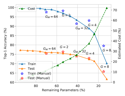
Figure 6: Change in ResNet-164 on CIFAR-100 accuracy while reducing number of parameters. Each sample point is collected from the model found by our model pruning algorithm under the given number of parameters constraint. Manually configured models either use uniform group size $G$ or set a maximum channel number $G_{M}$. The latter approach assigns each layer a group number that ensures $\max(C_{\text{in}}/G,C_{\text{out}}/G)\leq G_{M}$. We also list the estimated pruning cost for each explored sparsity configuration. Accuracy numbers listed here are collected from fine-tuning.

Group Configuration Exploration.

One of our major benefits is that we can explore group configuration under given inference budget constraints, as mentioned earlier. To evaluate the quality of the exploration, we gradually reduce the upper bound of number of parameters and run the model pruner. Results for ResNet-164 on CIFAR-100 are in Figure 6. The granularity of exploration here is 0.1M and we use the same training schedule for each sparsity configuration. Results demonstrate that explored models can perform on par with manually selected configurations.

ImageNet.

We evaluate various pre-trained ResNet models on ImageNet [8] . The fine-tuning phase has 30 epochs (1/3 of what [8] uses) with learning rate starting at $1e^{-3}$ and being multiplied by 0.1 every 10 epochs. Limited by hardware resources, we only select uniform numbers of groups.

Table 2: ImageNet evaluation results. The first sample in each section is the baseline.

Model	# Params.	# FLOPS	Top-1 Error
ResNet-18	11.69M	3.64G	30.24%
ResNet-18 $G$=8	1.91M	0.20G	44.71%
ResNet-18 $G$=8 [50]	1.91M	0.33G	44.60%
ResNet-34	21.80M	7.34G	26.70%
ResNet-34/A	17.36M	3.48G	28.42%
ResNet-34/B	9.05M	1.89G	32.44%
ResNet-34/A[32]	18.2M	3.98G	27.05%
ResNet-34/B[32]	11.1M	2.62G	27.75%
ResNet-50	25.56M	8.21G	23.85%
ResNet-50 $G$=2	13.82M	3.77G	25.90%
ResNet-101	44.55M	15.7G	22.63%
ResNet-101 $G$=2	23.34M	7.50G	24.22%

Results are listed in Table 2. Since models for ImageNet are rarely sparse, removing many parameters in one-shot normally degrades the accuracy significantly. For ResNet-18, we can reduce 83% parameters and 95% FLOPS with an increase of 14.5% in test error. It is not promising regarding the high test error, but this performance is on par with [50], even if they have higher budget in both training and inference phases: their ResNet-18 example is trained from scratch and the Hadamard transform adds overhead.

We also compare ResNet-34 to [32], which uses low-rank approximation to perform GConv pruning. This method requires adding pointwise $1\times 1$ convolution after each GConv. Since they use more parameters that potentially increase learning capacity, their accuracy can be higher. For the two configurations from [32], ResNet-34/A and /B, models produced by us are smaller but less accurate. However, as mentioned before, their GConv is always appended by a pointwise convolution, which means with the same number of groups they use more resources, and they cannot deal with $1\times 1$ group convolution. Specifically, for ResNet-50/101 that heavily uses $1\times 1$ kernels, our method can still reduce around 50% budget without increasing much test error.

4.3 Ablation Study

This section investigates the effect of different design choices that may appear while using our method.

Table 3: Comparison of the top-1 test error (%) between using the heuristic algorithm and not using (plain). ResNet-50 results are collected on ImageNet.

	heuristic		plain
Model	C10	C100	C10	C100
ResNet-110 ($G=2$)	6.69	27.63	7.13	28.08
ResNet-110 ($G=8$)	9.39	33.28	11.17	37.29
ResNet-50 ($G=2$)	25.90		28.04

Effect from heuristic algorithm.

We compare our algorithm with a plain algorithm, which tries to perform GConv pruning without sorting channels. Referring to Section 3.2, this plain algorithm simply sets $N_{S}$ to 0. This comparison is performed under the same group configuration to see whether our heuristic algorithm can improve the resulting accuracy. Table 3 presents the comparison between both approaches on ResNet-110 (CIFAR-10/100) and ResNet-50 (ImageNet) with uniform $G$. All experiments use the same training scheme (learning rate, number of epochs, etc.).

We notice that by using the heuristic algorithm, the test error of all variants on all datasets is reduced. This result is also in line with the relative order of recovery ratio as shown in Figure 5: $N_{S}$=0 has less recovery ratio than $N_{S}$=10 that is used by our heuristic algorithm, and it performs worse regarding the model accuracy. It can provide a concrete evidence that maximising recovery ratio, or equivalently minimising pruned magnitude, is an effective approach to conduct GConv pruning.

Table 4: Comparison between pruning and training from scratch for ResNet-164 on CIFAR-100 regarding top-1 train and test error.

	Train Err. (%)		Test Err. (%)
Method	$G$=2	$G$=4	$G$=2	$G$=4
Pruning	1.75	10.50	23.66	27.15
Shuffle	0.81	3.55	23.77	26.60
None	2.58	16.28	26.63	32.00

Compare with training from scratch.

Inspired by [25], we try to investigate that besides the reduction in training budget whether pruning can also achieve higher test accuracy than training from scratch. We focus on training GConv variants of ResNet-164 on CIFAR-100 by the same training from scratch schedule as [45]. These variants use uniform $G$ numbers 2 and 4, and they may use channel shuffle [49] to exchange information among groups or not. We also provide models with the same $G$ number produced by our pruning method.

Table 4 shows that overall training from scratch with channel shuffle performs better than other methods. Comparing pruning with channel shuffle, we notice that the difference in train error is much larger than test error, which implies that the worse performance from the pruning method may due to its improper training setup, e.g., the number of training epochs is too limited. But still, pruned models perform much better than their counterparts that are trained from scratch without channel permutation. It shows that the permutation of channels after GConv is indeed an important architectural choice.

4.4 Discussion

We show that our method can balance the trade-off between accuracy and workload size induced by group configuration through our efficient pruning algorithm, and improve the trade-off by rapid exploration of configurations under given constraints. Large and small models, small and large datasets are all covered. Compared with the state-of-the-art structured pruning methods [24, 12, 32], our approach is significantly better regarding its exploration ability and efficiency. Regarding model accuracy, we already perform on par with listed prior works, and we will try to surpass their results by tuning hyperparameters harder.

5 Conclusion

This paper proposes a novel pruning method that prunes a trained CNN model into one that is built on GConv. We formulate the layer-wise pruning problem as finding optimal permutations to incorporate the structural constraints imposed by GConv, and we efficiently solve it through our heuristic algorithm. We can further explore the best sparsity configuration of a whole model under specific inference budget constraints. Empirical results show that with given sparsity, our pruning algorithm can achieve competitive accuracy as other prior work with a shorter pruning period; and the sparsity configuration exploration, which used to be intractable, can be efficiently performed by our method.

Future work includes exploring different importance criteria to improve the quality of explored models, tuning the pruning hyperparameters to achieve higher model accuracy after the fine-tuning phase, and investigating the contribution of the regularisation effect on the better accuracy from CondenseNet. It is also possible to utilise NAS to improve our group configuration optimisation solution, since each group configuration basically determines an architecture.

References

- [1] Y. Chen, T. Yang, X. Zhang, G. Meng, C. Pan, and J. Sun. DetNAS: Neural Architecture Search on Object Detection. pages 1–11, 2019.
- [2] X. Dong, S. Chen, and S. J. Pan. Learning to Prune Deep Neural Networks via Layer-wise Optimal Brain Surgeon. In NeurIPS, 2017.
- [3] M. Figurnov, A. Ibraimova, D. Vetrov, and P. Kohli. PerforatedCNNs: Acceleration through Elimination of Redundant Convolutions. In NeurIPS, 2015.
- [4] R. S. Garfinkel and K. C. Gilbert. The Bottleneck Traveling Salesman Problem: Algorithms and Probabilistic Analysis. Journal of the ACM, 25(3):435–448, 1978.
- [5] S. Han, H. Mao, and W. J. Dally. Deep Compression - Compressing Deep Neural Networks with Pruning, Trained Quantization and Huffman Coding. In ICLR, 2016.
- [6] S. Han, J. Pool, J. Tran, and W. J. Dally. Learning Both Weights and Connections for Efficient Neural Networks. In NeurIPS, 2015.
- [7] B. Hassibi, D. G. Stork, and G. J. Wolff. Optimal brain surgeon and general network pruning. In IEEE International Conference on Neural Networks, 1993.
- [8] K. He, X. Zhang, S. Ren, and J. Sun. Deep Residual Learning for Image Recognition. In CVPR, 2016.
- [9] K. He, X. Zhang, S. Ren, and J. Sun. Identity Mappings in Deep Residual Networks. In ECCV, 2016.
- [10] A. G. Howard, M. Zhu, B. Chen, D. Kalenichenko, W. Wang, T. Weyand, M. Andreetto, and H. Adam. MobileNets: Efficient Convolutional Neural Networks for Mobile Vision Applications. CoRR, 2017.
- [11] H. Hu, R. Peng, Y.-W. Tai, and C.-K. Tang. Network Trimming: A Data-Driven Neuron Pruning Approach towards Efficient Deep Architectures. 2016.
- [12] G. Huang, S. Liu, L. van der Maaten, and K. Q. Weinberger. CondenseNet: An Efficient DenseNet using Learned Group Convolutions. CoRR, abs/1711.0, 2017.
- [13] G. Huang, Z. Liu, L. van der Maaten, and K. Q. Weinberger. Densely Connected Convolutional Networks. CoRR, abs/1608.0, 2016.
- [14] J. Huang, V. Rathod, C. Sun, M. Zhu, A. Korattikara, A. Fathi, I. Fischer, Z. Wojna, Y. Song, S. Guadarrama, and K. Murphy. Speed/accuracy trade-offs for modern convolutional object detectors. 2016.
- [15] Y. Ioannou, D. Robertson, R. Cipolla, and A. Criminisi. Deep Roots: Improving CNN Efficiency with Hierarchical Filter Groups. In CVPR, 2017.
- [16] A. Krizhevsky. Learning Multiple Layers of Features from Tiny Images. Technical report, 2009.
- [17] A. Krizhevsky, I. Sutskever, and G. E. Hinton. ImageNet Classification with Deep Convolutional Neural Networks. In NeurIPS, 2012.
- [18] V. Lebedev and V. Lempitsky. Fast ConvNets Using Group-Wise Brain Damage. In CVPR, pages 2554–2564, 2016.
- [19] Y. LeCun, J. S. Denker, and S. a. Solla. Optimal Brain Damage. In NeurIPS, pages 598–605, 1990.
- [20] H. Li, A. Kadav, I. Durdanovic, H. Samet, and H. P. Graf. Pruning Filters for Efficient Convnets. In ICLR, 2017.
- [21] C. Liu, B. Zoph, M. Neumann, J. Shlens, W. Hua, L. J. Li, L. Fei-Fei, A. Yuille, J. Huang, and K. Murphy. Progressive Neural Architecture Search. Lecture Notes in Computer Science (including subseries Lecture Notes in Artificial Intelligence and Lecture Notes in Bioinformatics), 11205 LNCS:19–35, 2018.
- [22] H. Liu, K. Simonyan, O. Vinyals, C. Fernando, and K. Kavukcuoglu. Hierarchical Representations for Efficient Architecture Search. In ICLR, 2018.
- [23] H. Liu, K. Simonyan, and Y. Yang. DARTS: Differentiable Architecture Search. In ICLR, 2019.
- [24] Z. Liu, J. Li, Z. Shen, G. Huang, S. Yan, and C. Zhang. Learning Efficient Convolutional Networks through Network Slimming. In ICCV, pages 2755–2763, 2017.
- [25] Z. Liu, M. Sun, T. Zhou, G. Huang, and T. Darrell. Rethinking the Value of Network Pruning. In ICLR, 2019.
- [26] J. H. Luo, J. Wu, and W. Lin. ThiNet: A Filter Level Pruning Method for Deep Neural Network Compression. In ICCV, 2017.
- [27] H. Mao, S. Han, J. Pool, W. Li, X. Liu, Y. Wang, and W. J. Dally. Exploring the Regularity of Sparse Structure in Convolutional Neural Networks. In NeurIPS, 2017.
- [28] M. Masana, J. V. D. Weijer, L. Herranz, A. D. Bagdanov, and J. M. Alvarez. Domain-Adaptive Deep Network Compression. In ICCV, pages 4299–4307, 2017.
- [29] P. Molchanov, S. Tyree, T. Karras, T. Aila, and J. Kautz. Pruning Convolutional Neural Networks for Resource Efficient Transfer Learning. In ICLR, 2017.
- [30] W. Pan, H. Dong, and Y. Guo. DropNeuron: Simplifying the Structure of Deep Neural Networks. In NeurIPS, 2016.
- [31] A. Paszke, G. Chanan, Z. Lin, S. Gross, E. Yang, L. Antiga, and Z. Devito. Automatic differentiation in PyTorch. In NeurIPS, 2017.
- [32] B. Peng, W. Tan, Z. Li, S. Zhang, D. Xie, and S. Pu. Extreme Network Compression via Filter Group Approximation. In ECCV, 2018.
- [33] E. Real, A. Aggarwal, Y. Huang, and Q. V. Le. Regularized Evolution for Image Classifier Architecture Search. pages 52–54, 2018.
- [34] O. Russakovsky, J. Deng, H. Su, J. Krause, S. Satheesh, S. Ma, Z. Huang, A. Karpathy, A. Khosla, M. Bernstein, A. C. Berg, and L. Fei-Fei. ImageNet Large Scale Visual Recognition Challenge. International Journal of Computer Vision, 115(3):211–252, 2015.
- [35] S. J. Russell and P. Norvig. Artificial Intelligence: A Modern Approach.
- [36] M. Sandler, A. Howard, M. Zhu, A. Zhmoginov, and L.-C. Chen. Inverted Residuals and Linear Bottlenecks: Mobile Networks for Classification, Detection and Segmentation. CoRR, 2018.
- [37] M. Tan, B. Chen, R. Pang, V. Vasudevan, M. Sandler, A. Howard, and Q. V. Le. MnasNet: Platform-Aware Neural Architecture Search for Mobile. 2018.
- [38] M. Tan and Q. V. Le. EfficientNet: Rethinking Model Scaling for Convolutional Neural Networks. In ICML, 2019.
- [39] X. Wang, M. Kan, S. Shan, and X. Chen. Fully Learnable Group Convolution for Acceleration of Deep Neural Networks. In CVPR, pages 9049–9058, 2019.
- [40] W. Wen, C. Wu, Y. Wang, Y. Chen, and H. Li. Learning Structured Sparsity in Deep Neural Networks. In NeurIPS, 2016.
- [41] R. J. Williams. Simple statistical gradient-following algorithms for connectionist reinforcement learning. Machine Learning, 8(3-4):229–256, 1992.
- [42] G. Xie, J. Wang, T. Zhang, J. Lai, R. Hong, and G.-J. Qi. IGCV$2$: Interleaved Structured Sparse Convolutional Neural Networks. 2018.
- [43] G. Xie, J. Wang, T. Zhang, J. Lai, R. Hong, and G.-J. Qi. Interleaved Structured Sparse Convolutional Neural Networks. In CVPR, 2018.
- [44] S. Xie, R. Girshick, P. Dollár, Z. Tu, and K. He. Aggregated Residual Transformations for Deep Neural Networks. In CVPR, 2017.
- [45] W. Yang. Pytorch classification. https://github.com/bearpaw/pytorch-classification.
- [46] R. Yu, A. Li, C.-F. Chen, J.-H. Lai, V. I. Morariu, X. Han, M. Gao, C.-Y. Lin, and L. S. Davis. NISP: Pruning Networks using Neuron Importance Score Propagation. In CVPR, 2018.
- [47] M. Yuan and Y. Lin. Model selection and estimation in regression with grouped variables. Journal of the Royal Statistical Society. Series B: Statistical Methodology, 68(1):49–67, 2006.
- [48] T. Zhang, G.-J. Qi, B. Xiao, and J. Wang. Interleaved Group Convolutions for Deep Neural Networks. In ICCV, 2017.
- [49] X. Zhang, X. Zhou, M. Lin, and J. Sun. ShuffleNet: An Extremely Efficient Convolutional Neural Network for Mobile Devices. CoRR, 2017.
- [50] R. Zhao, Y. Hu, J. Dotzel, C. De Sa, and Z. Zhang. Building Efficient Deep Neural Networks with Unitary Group Convolutions. 2018.
- [51] B. Zoph and Q. V. Le. Neural Architecture Search with Reinforcement Learning. CoRR, pages 1–16, 2016.
- [52] B. Zoph, V. Vasudevan, J. Shlens, and Q. V. Le. Learning Transferable Architectures for Scalable Image Recognition. 2017.