Ladder operators and coherent states for multi-step supersymmetric rational extensions of the truncated oscillator

Abstract

We construct ladder operators, $\tilde{C}$ and $\tilde{C}^{\dagger},$ for a multi-step rational extension of the harmonic oscillator on the half plane, $x\geq 0.$ These ladder operators connect all states of the spectrum in only infinite-dimensional representations of their polynomial Heisenberg algebra. For comparison, we also construct two different classes of ladder operator acting on this system that form finite-dimensional as well as infinite-dimensional representations of their respective polynomial Heisenberg algebras. For the rational extension, we construct the position wavefunctions in terms of exceptional orthogonal polynomials. For a particular choice of parameters, we construct the coherent states, eigenvectors of $\tilde{C}$ with generally complex eigenvalues, $z,$ as superpositions of a subset of the energy eigenvectors. Then we calculate the properties of these coherent states, looking for classical or non-classical behaviour. We calculate the energy expectation as a function of $|z|.$ We plot position probability densities for the coherent states and for the even and odd cat states formed from these coherent states. We plot the Wigner function for a particular choice of $z.$ For these coherent states on one arm of a beamsplitter, we calculate the two excitation number distribution and the linear entropy of the output state. We plot the standard deviations in $x$ and $p$ and find no squeezing in the regime considered. By plotting the Mandel $Q$ parameter for the coherent states as a function of $|z|,$ we find that the number statistics is sub-Poissonian.

I Introduction

Supersymmetric quantum mechanics Witten1981 ; Witten1982 ; Mielnik1984 ; Adrianov1993 ; Adrianov1995 ; Cooper1995 ; Fernandez1998a ; Fernandez1998b ; Samsonov1999 ; Mielnick2000 ; Carinena2001 ; Aoyama2001 ; Carballo2004 ; Marquette2009 ; Fernandez2010 ; Quesne2011 ; Marquette2012 ; GomezUllate2014 has been widely used to create partner Hamiltonians for a given, exactly solvable, Hamiltonian that have at least part of the spectrum in common with the original. Typically there are one or more energy levels of the partner Hamiltonian below the ground state energy of the original Hamiltonian.

In this paper, following Marquette2014b , we consider multi-step rational extensions of the harmonic oscillator. The novel aspect of this paper is that we consider multi-step rational extensions of the truncated oscillator, confined to the half plane $x\geq 0,$ with the potential being infinite for $x<0.$ This potential has been considered by other authors Fernandez2014 ; Fernandez2016 , but not with multi-step rational extensions. Fernández C. et al. Fernandez2018b considered the truncated oscillator with the same rational extension that we use. They constructed coherent states associated with linearized versions of the ladder operators we label $\widetilde{L}$ and $\widetilde{L}^{\dagger}$ in Section II below.

In Section II, we review the construction of the partner Hamiltonian in the untruncated case and the construction of three types of ladder operator that connect the energy levels. Then we consider the truncated case, which eliminates all states with position wavefunctions even in $x.$ We construct three types of ladder operator that connect the energy levels of the truncated system. We will find, below, that there is significant structure to the energy levels, such that some of the levels are singlets or doublets under the action of the various ladder operators. In every case there are also infinite dimensional representations of the polynomial Heisenberg algebras.

We note that the potential we are considering is singular, taking an infinite value for all $x<0.$ Other work has been done on potentials with singularities Marquez1998 .

In Section III we construct coherent states associated with the ladder operators we label $(\tilde{C},\tilde{C}^{\dagger}).$ Coherent states are of widespread interest Glauber1963a ; Glauber1963b ; Klauder1963a ; Klauder1963b ; Barut1971 ; Perelomov1986 ; Gazeau1999 ; Quesne2001 ; Fernandez1995 ; Fernandez1999 ; GomezUllate2014 ; Ali2014 because they can, in some cases, be the quantum-mechanical states with the most classical behaviour. Then we systematically investigate properties of these coherent states, looking for classical or non-classical behaviour. We calculate the energy expectation as a function of $|z|,$ where $z$ is the generally complex coherent state parameter. We calculate position probability densities for a particular choice of parameters. A similar calculation is done for even and odd cat states. We plot the Wigner function, an accepted measure of classicality, for a particular choice of parameters. For our coherent state on one arm of a beamsplitter, we calculate the two excitation (“photon”) number distribution and look for factorizability. We calculate the linear entropy of the output state as a measure of entanglement. We calculate the standard deviations in position and momentum over a range of $z$ values to look for squeezing and to confirm the Heisenberg uncertainty principle. Lastly, we calculate the Mandel $Q$ parameter for these coherent states as a function of $|z|$ to characterize the number statistics.

In Section IV, we compare our results with those of Fernández C. et al. Fernandez2018b .

Conclusions follow in Section IV.

II Theory of multi-step rational extensions of the harmonic oscillator

II.1 The untruncated oscillator

We scale the harmonic oscillator Hamiltonian,

$$H_{HO}=-\frac{\hbar^{2}}{2m}\frac{d^{2}}{dx^{2}}+\frac{1}{2}m\omega^{2}x^{2},$$ (II.1)

according to $\hbar=1,$ $m=1/2,$ $\omega=2,$ to give the (1) Hamiltonian

$$H^{(1)}=-\frac{d^{2}}{dx^{2}}+x^{2},$$ (II.2)

with energy levels $E_{\nu}^{(1)}=2\nu+1$ for $\nu=0,1,2,\dots.$ The annihilation and creation operators are, respectively,

$$a=\frac{d}{dx}+x,\quad a^{\dagger}=-\frac{d}{dx}+x$$ (II.3)

satisfying the Heisenberg algebra

$$[H^{(1)},a^{\dagger}]=2a^{\dagger},\quad[H^{(1)},a]=-2a,\quad[a,a^{\dagger}]=2.$$ (II.4)

We first present the $k$-step construction for the untruncated oscillator, for $x$ on the entire real axis, following the results of Marquette2014b on Darboux-Crum (state adding) and Krein-Adler (state deleting) SUSY QM. The class of example chains we will consider in this paper is given by consecutive values of $m:$

$$\{m_{1},m_{2},\dots,m_{k-1},m_{k}\}=\{2,3,\dots,k,k+1\},$$ (II.5)

with $k$ even.

We choose for the state adding case the following seed solutions

$$\phi_{m_{1}}(x)=\mathcal{H}_{m_{1}}(x)\,e^{x^{2}/2},\dots,\phi_{m_{k}}(x)=\mathcal{H}_{m_{k}}(x)\,e^{x^{2}/2},$$ (II.6)

where

$$\mathcal{H}_{m}(x)=(-i)^{m}H_{m}(ix)$$ (II.7)

are the modified Hermite polynomials in terms of the standard Hermite polynomials $H_{m}(x)$ Gradsteyn1980 . First we define

$$Q^{(1)} =\phi_{m_{1}},$$

$$Q^{(i)} =\frac{\mathcal{W}(\phi_{m_{1}},\dots,\phi_{m_{i}})}{\mathcal{W}(\phi_{m_{1}},\dots,\phi_{m_{i-1}})}\quad\mathrm{for}\ i=2,\dots,k,$$ (II.8)

where $\mathcal{W}$ indicates the Wronskian determinant

$$\mathcal{W}(\phi_{1},\phi_{2},\dots,\phi_{n})=\det\begin{pmatrix}\phi_{1}&\phi_{2}&\dots&\phi_{n}\\ \phi_{1}^{(1)}&\phi_{2}^{(1)}&\dots&\phi_{n}^{(1)}\\ \dots&\dots&\dots&\dots\\ \phi_{1}^{(n-1)}&\phi_{2}^{(n-1)}&\dots&\phi_{n}^{(n-1)}\end{pmatrix}.$$ (II.9)

The supercharges, $A^{(i)},$ are given by

$$A^{(i)} =\frac{d}{dx}+W^{(i)}\quad\mathrm{for}\ i=1,\dots,k,$$ (II.10)

with

$$W^{(i)}=-\frac{d}{dx}\ln Q^{(i)}\quad\mathrm{for}\ i=1,\dots,k.$$ (II.11)

The product of these supercharges is

$$A =A^{(k)}A^{(k-1)}\dots A^{(1)}.$$ (II.12)

It is not the case here that $H^{(1)}=A^{\dagger}A,H^{(2)}=AA^{\dagger},$ as in simpler examples of supersymmetry with first-order supercharges. However we require that the intertwining relation,

$$A\,H^{(1)}=H^{(2)}\,A,$$ (II.13)

hold and relate the initial Hamiltonian $H^{(1)}$ (the harmonic oscillator) to a final Hamiltonian $H^{(2)}$ through a chain of Hamiltonians, alternately regular and singular. We solve this relation to give

$$H^{(1)} =-\frac{d^{2}}{dx^{2}}+x^{2},\quad H^{(2)}=-\frac{d^{2}}{dx^{2}}+V^{(2)},$$

$$V^{(2)} =x^{2}-2\frac{d^{2}}{dx^{2}}\ln\mathcal{W}(\phi_{m_{1}},\dots,\phi_{m_{k}})+\Delta E.$$ (II.14)

We know the wavefunctions of $H^{(1)}$

$$\psi_{\nu}=H_{\nu}\,e^{-x^{2}/2},$$ (II.15)

with energies $E_{\nu}^{(1)}=2\nu+1,\ \mathrm{for}\ \nu=0,1,2,\dots.$ The partner Hamiltonian wavefunctions can be written in terms of the seed solutions

$$\psi_{\nu}^{(2)} \propto\mathcal{W}(\phi_{m_{1}},\dots,\phi_{m_{k}},\psi_{\nu})\quad\mathrm{for}\ \nu=0,1,2,\dots,$$

$$\psi_{-m_{i}-1}^{(2)} \propto\mathcal{W}(\phi_{m_{1}},\dots,\check{\phi}_{m_{i}},\dots,\phi_{m_{k}})\quad\mathrm{for}\ i=1,2,\dots,k,$$ (II.16)

where $\mathcal{W}(\phi_{m_{1}},\dots,\check{\phi}_{m_{i}},\dots,\phi_{m_{k}})$ means $\phi_{m_{i}}$ is missing from the sequence. Here $\psi_{\nu}^{(2)}$ are the states obtained from $\psi_{\nu}^{(1)}$ by $A\psi_{\nu}^{(1)}.$ The other states, $\psi_{-m_{i}-1}^{(2)},$ are obtained via the constraint $A^{\dagger}\psi=0.$ Here $A^{\dagger}$ is a $k-$th order differential operator and there is more than one zero mode.

The energy levels are $E_{\nu}^{(2)}=2\nu+1$ for $\nu=-m_{k}-1,-m_{k-1}-1,\dots,-m_{1}-1,0,1,2,\dots.$

The other construction (state deleting) uses only the seed solutions $\{\psi_{k},\psi_{k+1}\},$ with the other states having been deleted.

We construct the supercharges and superpotentials in a similar way to what was done in the first construction, starting with

$$\bar{Q}^{(k)} =\psi_{k},$$

$$\bar{Q}^{(k+1)} =\frac{\mathcal{W}(\psi_{k},\psi_{k+1})}{\psi_{k}}.$$ (II.17)

Then

$$\overline{W}^{(i)}=-\frac{d}{dx}\ln\overline{Q}^{(i)}\quad\mathrm{for}\ i=k,k+1,$$ (II.18)

$$\overline{A}^{(i)} =\frac{d}{dx}+\overline{W}^{(i)}\quad\mathrm{for}\ i=k,k+1,$$ (II.19)

and

$$\overline{A}=\overline{A}^{(k+1)}\overline{A}^{(k)}.$$ (II.20)

The partner Hamiltonian is again equal to $H^{(2)}$ as in Eq. (II.14), found by solving the intertwining relation

$$\overline{A}\,H^{(1)}=H^{(2)}\,\overline{A}$$ (II.21)

with an appropriate energy shift. The wavefunctions and energy levels are then the same as in the previous construction Marquette2014b .

Two types of standard ladder operators can be generated, $(L^{\dagger},L)$ and $(\bar{L}^{\dagger},\bar{L}),$ given by

$$L^{\dagger} =Aa^{\dagger}A^{\dagger},\quad L=AaA^{\dagger},$$ (II.22)

and

$$\bar{L}^{\dagger} =\bar{A}a^{\dagger}\bar{A}^{\dagger},\quad\bar{L}=\bar{A}a\bar{A}^{\dagger}.$$ (II.23)

We find that the commutators for $(L^{\dagger},L)$ are

$$[H^{(2)},L^{\dagger}] =2L^{\dagger},\quad[H^{(2)},L]=-2L,\quad[L,L^{\dagger}]=P(H^{(2)}+2)-P(H^{(2)}),$$ (II.24)

with

$$P(H^{(2)})=\prod_{i=1}^{k}(H^{(2)}+2m_{i}-1)(H^{(2)}-1)\prod_{j=1}^{k}(H^{(2)}+2m_{j}+1).$$ (II.25)

We find that the commutators for $(\bar{L}^{\dagger},\bar{L})$ are

$$[H^{(2)},\bar{L}^{\dagger}] =2\bar{L}^{\dagger},\quad[H^{(2)},\bar{L}]=-2\bar{L},\quad[\bar{L},\bar{L}^{\dagger}]=\bar{P}(H^{(2)}+2)-\bar{P}(H^{(2)}),$$ (II.26)

with

$$\bar{P}(H^{(2)})=\prod_{i=1}^{m_{k}}(H^{(2)}+2m_{k}-2i-1)(H^{(2)}+2m_{k}+1)\prod_{j=1}^{m_{k}}(H^{(2)}+2m_{k}-2j+1),$$ (II.27)

for $j\neq m_{k}-m_{k-1},\dots,m_{k}-m_{1}.$

The combination of both Darboux-Crum and Krein-Adler paths can be exploited to generate a different type of ladder operator, the type we will focus on in this paper,

$$C =\bar{A}A^{\dagger},\quad C^{\dagger}=A\bar{A}^{\dagger}.$$ (II.28)

We find that the commutators are

$$[H^{(2)},C^{\dagger}] =(2m_{k}+2)C^{\dagger},\quad[H^{(2)},C]=-(2m_{k}+2)C,\quad[C,C^{\dagger}]=Q(H^{(2)}+2m_{k}+2)-Q(H^{(2)}),$$ (II.29)

with

$$Q(H^{(2)})=\prod_{i=1}^{k}(H^{(2)}+2m_{i}+1)\prod_{j\neq m_{k}-m_{k-1},\dots,m_{k}-m_{1}}^{m_{k}}(H^{(2)}-2j-1).$$ (II.30)

The zero modes of $(C,C^{\dagger}),(L,L^{\dagger})$ and $(\bar{L},\bar{L}^{\dagger})$ are associated with the energies for which $Q,P$ and $\bar{P}$ and $Q(H^{(2)}+2m_{k}+2),P(H^{(2)}+2)$ and $\bar{P}(H^{(2)}+2)$ vanish.

In this paper we will consider the untruncated and truncated oscillators and their supersymmetric partners for the particular choice

$$\{m_{1},m_{2},m_{3},m_{4}\}=\{2,3,4,5\}.$$ (II.31)

We find that the partner potential is

$$V^{(2)} =-8+x^{2}-\frac{1024(-315+90x^{2}-1020x^{4}+328x^{6})}{(45+120x^{4}-64x^{6}+16x^{8})^{2}}+$$

$$\quad+\frac{64(-112-13x^{2}-4x^{4}+4x^{6})}{45+120x^{4}-64x^{6}+16x^{8}}.$$ (II.32)

This is in full agreement with Fernandez2018 , after noting that their Hamiltonians are one half of ours.

The first (state adding) path uses

$$Q^{(1)} =e^{x^{2}/2}(2+4x^{2}),$$

$$Q^{(2)} =8e^{x^{2}/2}\frac{3+4x^{2}}{2+4x^{2}},$$

$$Q^{(3)} =16e^{x^{2}/2}\frac{9+18x^{2}-12x^{4}+8x^{6}}{3+4x^{4}},$$

$$Q^{(4)} =96e^{x^{2}/2}\frac{9+18x^{2}(15-8x^{2}+2x^{4})}{9+18x^{2}-12x^{4}+8x^{6}}.$$ (II.33)

The second (state deleting) path uses

$$\bar{Q}^{(4)} =e^{-x^{2}/2}(12-48x^{2}+16x^{4}),$$

$$\bar{Q}^{(5)} =8e^{-x^{2}/2}\frac{(45+8x^{4}(15-8x^{2}+2x^{4}))}{3-12x^{2}+4x^{4}}.$$ (II.34)

We can form the $C,L$ and $\bar{L}$ ladder operators from

$$C =\bar{A}^{(5)}\bar{A}^{(4)}A^{(1)\dagger}A^{(2)\dagger}A^{(3)\dagger}A^{(4)\dagger},$$

$$L =A^{(4)}A^{(3)}A^{(2)}A^{(1)}aA^{(1)\dagger}A^{(2)\dagger}A^{(3)\dagger}A^{(4)\dagger},$$

$$\bar{L} =\bar{A}^{(5)}\bar{A}^{(4)}a\bar{A}^{(4)\dagger}\bar{A}^{(5)\dagger}.$$ (II.35)

Then $C^{\dagger},L^{\dagger}$ and $\bar{L^{\dagger}}$ are just the respective Hermitian conjugates. For $\{l_{1},l_{2},l_{3}\}=\{C,L,\bar{L}\},$ the polynomial Heisenberg algebras that they satisfy take the forms for our particular model

$$[H^{(2)},l_{n}]=-\lambda_{n}l_{n},\quad[H^{(2)},l_{n}^{\dagger}]=+\lambda_{n}l_{n}^{\dagger},\quad[l_{n},l_{n}^{\dagger}]=P_{n}(H^{(2)}+\lambda_{n})-P_{n}(H^{(2)}),$$ (II.36)

with

$$\{\lambda_{1},\lambda_{2},\lambda_{3}\}=\{2,2,12\},$$ (II.37)

and

$$P_{1}(H^{(2)}) =(H^{(2)}-11)(H^{(2)}-9)(H^{(2)}+5)(H^{(2)}+7)(H^{(2)}+9)(H^{(2)}+11),$$

$$P_{2}(H^{(2)}) =(H^{(2)}+3)(H^{(2)}+5)(H^{(2)}+7)(H^{(2)}+9)(H^{(2)}-1)(H^{(2)}+5)(H^{(2)}+7)(H^{(2)}+9)(H^{(2)}+11),$$

$$P_{3}(H^{(2)}) =(H^{(2)}+11)(H^{(2)}+1)(H^{(2)}-1)(H^{(2)}+3)(H^{(2)}+1).$$ (II.38)

The zero modes of the ladder operators are given in Table 1.

Ladder operator	Zero modes
$C$	$\psi_{-6}^{(2)},\psi_{-5}^{(2)},\psi_{-4}^{(2)},\psi_{-3}^{(2)},\psi_{4}^{(2)},\psi_{5}^{(2)}$
$C^{\dagger}$	No physical states
$L$	$\psi_{-6}^{(2)},\psi_{-5}^{(2)},\psi_{-4}^{(2)},\psi_{-3}^{(2)},\psi_{0}^{(2)}$
$L^{\dagger}$	$\psi_{-6}^{(2)},\psi_{-5}^{(2)},\psi_{-4}^{(2)},\psi_{-3}^{(2)}$
$\bar{L}$	$\psi_{-6}^{(2)},\psi_{0}^{(2)}$
$\bar{L}^{\dagger}$	$\psi_{-3}^{(2)}$

Table 1: Zero modes of the six ladder operators for the untruncated system.

The energy levels of $H^{(2)}$ are given by $E_{\nu}^{(2)}=2\nu+1\quad\mathrm{for}\ \nu=-6,-5,-4,-3,0,1,2,\dots.$ (Note we do not apply an energy shift here to make all energies positive).

In Figure 1 we show the physical states and the actions of the three types of ladder operator for the untruncated case we are considering. We note that $(L,L^{\dagger})$ and $(\bar{L},\bar{L}^{\dagger})$ have finite-dimensional as well as infinite-dimension representations of their respective polynomial Heisenberg algebras, while $(C,C^{\dagger})$ have only infinite-dimensional representations.

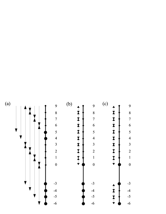
Figure 1: Physical states and actions of the ladder operators (a) $C,C^{\dagger},$ (b) $L,L^{\dagger}$ and (c) $\bar{L},\bar{L}^{\dagger}.$ The large dots represent zero modes of either raising or lowering operators in each case.

II.2 The truncated oscillator

The truncated oscillator has Hamiltonian

$$\tilde{H}^{(1)}=\begin{cases}-\frac{d^{2}}{dx^{2}}+x^{2}&0\leq x<\infty,\\ \infty&x<0.\end{cases}$$ (II.39)

In this case only the odd states from the previous derivation (Section II. A) are the physical states with wavefunctions satisfying the boundary condition of vanishing at the origin. To obtain the truncated supersymmetric partner we also select the physical states which satisfy the boundary condition. SUSY QM might only be formal if the boundary condition of the Hamiltonian and superpartner are not the same.

The physical state wavefunctions of $\tilde{H}^{(1)}$ are

$$\tilde{\psi}_{1}^{(1)} =2x\,e^{-x^{2}/2},$$

$$\tilde{\psi}_{3}^{(1)} =(-12x+8x^{3})\,e^{-x^{2}/2},$$

$$\tilde{\psi}_{5}^{(1)} =(120x-160x^{3}+32x^{5})\,e^{-x^{2}/2},$$ (II.40)

$$\dots$$

with energies $\tilde{E}_{\nu}^{(1)}=2\nu+1,\ \mathrm{for}\ \nu=1,3,5,\dots.$ For the superpartner, they are

$$\psi_{-5}^{(2)},\quad\tilde{E}_{-5}^{(2)} =-9,$$

$$\psi_{-3}^{(2)},\quad\tilde{E}_{-3}^{(2)} =-5,$$

$$\psi_{1}^{(2)},\quad E_{1}^{(2)} =3,$$

$$\psi_{3}^{(2)},\quad\tilde{E}_{3}^{(2)} =7,$$

$$\dots$$ (II.41)

with the $\psi_{\nu}^{(2)}$ wavefunctions given by Eq. (II.16).

The ladder operators $C^{\dagger}$ and $C$ change the index by $\pm 6,$ respectively, an even number, so they transform odd states into odd states and even states into even states. Thus they split the state space into two distinct, irreducible representations. Hence the ladder operators $\tilde{C}$ and $\tilde{C}^{\dagger}$ for the truncated oscillator can be taken as $C$ and $C^{\dagger},$ respectively, restricted to the odd subspace.

The ladder operators $L^{\dagger},L,\bar{L}^{\dagger}$ and $\bar{L}$ change the index by $\pm 1,$ mixing odd states and even states. Thus we construct new lowering operators for the truncated oscillator that change the index by $-2$:

$$\widetilde{L} =Aa^{2}A^{\dagger},$$

$$\widetilde{\bar{L}} =\bar{A}a^{2}\bar{A}^{\dagger},$$ (II.42)

with the raising operators given by the Hermitian conjugates, which change the index by $+2$. The polynomial Heisenberg algebras take the forms

$$[\widetilde{H}^{(2)},\widetilde{L}] =-4\widetilde{L},\quad[\widetilde{H}^{(2)},\widetilde{L}^{\dagger}]=4\widetilde{L}^{\dagger},$$

$${}[\widetilde{L},\widetilde{L}^{\dagger}] =\widetilde{P(}\widetilde{H}^{(2)}+4)-\widetilde{P(}\widetilde{H}^{(2)})$$ (II.43)

and

$$[\widetilde{H}^{(2)},\widetilde{\bar{L}}] =-4\widetilde{\bar{L}},\quad[\widetilde{H}^{(2)},\widetilde{\bar{L}}^{\dagger}]=4\widetilde{\bar{L}}^{\dagger},$$

$${}[\widetilde{\bar{L}},\widetilde{\bar{L}}^{\dagger}] =\widetilde{\bar{P}(}\widetilde{H}^{(2)}+4)-\widetilde{\bar{P}(}\widetilde{H}^{(2)}).$$ (II.44)

In these expressions

$$\widetilde{P(}\widetilde{H}^{(2)}) =(\widetilde{H}^{(2)}+1)(\widetilde{H}^{(2)}+3)(\widetilde{H}^{(2)}+5)(\widetilde{H}^{(2)}+7)(\widetilde{H}^{(2)}-5)\times$$

$$\quad\times(\widetilde{H}^{(2)}-3)(\widetilde{H}^{(2)}+5)(\widetilde{H}^{(2)}+7)(\widetilde{H}^{(2)}+9)(\widetilde{H}^{(2)}+11),$$

$$\widetilde{\bar{P}(}\widetilde{H}^{(2)}) =(\widetilde{H}^{(2)}+9)(\widetilde{H}^{(2)}-1)(\widetilde{H}^{(2)}+11)(\widetilde{H}^{(2)}-3)(\widetilde{H}^{(2)}+3)(\widetilde{H}^{(2)}+1).$$ (II.45)

The zero modes are shown in Table 2.

Ladder operator	Zero modes
$\tilde{C}$	$\psi_{-5}^{(2)},\psi_{-3}^{(2)},\psi_{5}^{(2)}$
$\tilde{C}^{\dagger}$	No physical states
$\tilde{L}$	$\psi_{-5}^{(2)},\psi_{-3}^{(2)},\psi_{1}^{(2)}$
$\tilde{L}^{\dagger}$	$\psi_{-5}^{(2)},\psi_{-3}^{(2)}$
$\widetilde{\bar{L}}$	$\psi_{-5}^{(2)},\psi_{1}^{(2)}$
$\widetilde{\bar{L}}^{\dagger}$	$\psi_{-3}^{(2)}$

Table 2: Zero modes of four ladder operators for the truncated system.

In Figure 2 we show the physical states and the actions of the three types of ladder operator for the truncated case we are considering. We see that only the ladder operators $(\tilde{C},\tilde{C}^{\dagger})$ have only infinite-dimensional representations.

Figure 2: Physical states and actions of the ladder operators (a) $\tilde{C},\tilde{C}^{\dagger},$ (b) $\tilde{L},\tilde{L}^{\dagger}$ and (c) $\widetilde{\bar{L}},\widetilde{\bar{L}}^{\dagger}.$ The large dots represent zero modes of either raising or lowering operators in each case.

III Construction and properties of coherent states

We construct the coherent states associated with the ladder operators $(\tilde{C},\tilde{C}^{\dagger})$ for the particular case of lowest weight $\mu=5.$

For $\mu=5,$ the matrix elements of $\tilde{C},$ as given in Marquette2014b , are

$$\langle\,5+6i-6\,|\,\tilde{C}\,|\,5+6i\,\rangle=a_{5+6i}=[2^{6}(11+6i)\frac{(4+6i)!}{(6i-1)!}\frac{8+6i}{2+6i}\frac{9+6i}{3+6i}\frac{10+6i}{4+6i}]^{\frac{1}{2}},\quad\mathrm{for}\ i=1,2,3,\dots.$$ (III.1)

Using similar results from Hoffmann2018c , the coherent states with the Barut-Girardello definition Barut1971 as eigenvectors of the lowering operator with generally complex eigenvalues,

$$\tilde{C}\,|\,z;c,5\,\rangle=z\,|\,z;c,5\,\rangle,$$ (III.2)

are given by

$$|\,z;c,5\,\rangle=\sum_{k=0}^{\infty}|\,5+6k\,\rangle\alpha_{k}^{(5)}$$ (III.3)

with

$$\alpha_{k}^{(5)}(z)=\frac{1}{\sqrt{F^{(5)}(z)}}\frac{z^{k}}{D_{k}^{(5)}}.$$ (III.4)

Here

$$D_{0}^{(5)}=1,\quad D_{k}^{(5)}=\prod_{i=1}^{k}a_{5+6i}\quad\mathrm{for}\ k\geq 1$$ (III.5)

and

$$F^{(5)}(z)=\sum_{k=0}^{\infty}\frac{|z|^{2k}}{D_{k}^{(5)2}}.$$ (III.6)

III.1 Energy expectation

We first calculate the energy expectation as a function of $|z|$ for this coherent state. This is

$$\langle\,E^{(5)}(|z|)\,\rangle=\langle\,z;c,5\,|\,H^{(2)}\,|\,z;c,5\,\rangle=11+\frac{12}{F^{(5)}(z)}\sum_{k=0}^{\infty}k\frac{|z|^{2k}}{D_{k}^{(5)2}}.$$ (III.7)

The denominators grow very rapidly: $D_{k}^{(5)2}=1,1.5\times 10^{8},3.3\times 10^{17},4.1\times 10^{27}$ for $k=0,1,2,3.$ We take the sum to $k=6$ with negligible remainder. As a consequence, $F^{(5)}(z)$ and $\langle\,E^{(5)}(z)\,\rangle$ grow very slowly for low values of $|z|.$ We find the following profile up to $|z|=10^{5},$ as shown in Fig. 3. Fernández C. et al. Fernandez2018b did not calculate the energy expectation.

Figure 3: Energy expectation for the coherent states with $\mu=5.$

III.2 Position probability densities

According to Marquette and Quesne Marquette2014b , the unnormalized wavefunctions are

$$\Psi_{\nu}^{(2)}(x)=\frac{\mathcal{W}(\phi_{2},\phi_{3},\phi_{4},\phi_{5},\psi_{\nu})}{\mathcal{W}(\phi_{2},\phi_{3},\phi_{4},\phi_{5})},\quad\mathrm{where}\ \psi_{\nu}(x)=H_{\nu}(x)\,e^{-x^{2}/2}.$$ (III.8)

We need to calculate

$$\mathcal{N}_{\nu}=\int_{0}^{\infty}dx\,|\Psi_{\nu}^{(-)}(x)|^{2}$$ (III.9)

(for normalization on the half line) and then form the normalized wavefunctions

$$\psi_{\nu}^{(-)}(x)=\frac{\Psi_{\nu}^{(-)}(x)}{\sqrt{\mathcal{N}_{\nu}}}.$$ (III.10)

Then the probability density for the coherent state is

$$\rho(x,t;z,5)=|\langle\,x\,|\,e^{-iH^{(2)}t}\,|\,z;c,5\,\rangle|^{2}=\left|\sum_{k=0}^{\infty}\psi_{5+6k}^{(-)}(x)\frac{1}{\sqrt{F^{(5)}(z)}}\frac{(z\,e^{-i12t})^{k}}{D_{k}^{(5)}}\right|^{2}.$$ (III.11)

For $|z|\leq 10^{5},$ we can take the sum to $k=11.$ The density plot over one period is shown in Figure 4. We see considerable structure, with individual wavepackets diminishing and reforming.

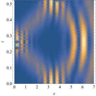
Figure 4: Density plot of $\rho(x,t;10^{5},5)$ over one period.

III.3 Even and odd cat states

The distinguishability measure in this case is

$$D^{(5)}(z) =\langle\,-z;c,5\,|\,+z;c,5\,\rangle=\frac{1}{F^{(5)}(z)}\sum_{k=0}^{\infty}(-)^{k}\frac{|z|^{2k}}{D_{k}^{(5)2}}.$$ (III.12)

This function is plotted in Figure 5. We see that the distinguishability falls to zero as $|z|\rightarrow\infty,$ but there are also two other zeros at finite values of $|z|.$

Figure 5: Distinguishability measure $D^{(5)}(|z|).$

We form the cat states (approximately normalized)

$$|\,z;+,c,5\,\rangle =\frac{1}{\sqrt{2}}\{|\,+z;c,5\,\rangle+|\,-z;c,5\,\rangle\},\quad|\,z;-,c,5\,\rangle=\frac{1}{\sqrt{2}}\{|\,+z;c,5\,\rangle-|\,-z;c,5\,\rangle\},$$ (III.13)

and plot their time-dependent probability densities for $z=10^{5}$ (to ensure distinguishability) in Figure 6. (Again, we take the sum over $k$ to $k=11.$) Here, too, we see a great deal of structure.

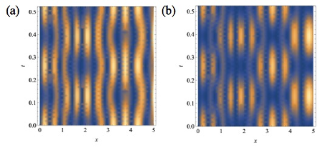
Figure 6: Time-dependent densities for (a) the + and (b) the - cat states, with $z=10^{5}$.

III.4 Wigner function

We use the formula for the Wigner function Hoffmann2018c

$$W(x,p;z,5)=\sum_{k_{1}=0}^{\infty}\sum_{k_{2}=0}^{\infty}\alpha_{k_{1}}^{(5)*}(z)w_{k_{1}k_{2}}(x,p)\alpha_{k_{2}}^{(5)}(z)$$ (III.14)

with

$$w_{k_{1}k_{2}}(x,p)=\begin{cases}\frac{1}{\pi}\int_{-x}^{x}dy\,\psi_{5+6k_{1}}^{(-)*}(x-y)\psi_{5+6k_{2}}^{(-)}(x+y)e^{-i2py}&x>0,\\ 0&x<0\end{cases}$$ (III.15)

in this truncated case. The integrand can only be nonzero for $x-y>0$ and $x+y>0.$ This gives $-x<y<x$ for positive $x$ and no region of nonzero integrand for negative $x.$

For $z=500,$ we assume the $k_{1}=k_{2}=0$ contribution is sufficient because of the rapid decrease with $k$ of the coefficients $\alpha_{k}^{(5)}(500)$. We find the Wigner function displayed in Figure 7, vanishing for negative $x$. Closer inspection shows only small areas of small negative Wigner function $(W(1.9,0.8;500,5)=-0.036)$, which may disappear if we improve our approximation. We conclude that there is no clear signature of non-classical behaviour.

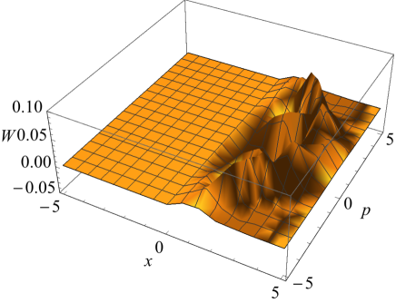
Figure 7: Wigner function for $z=500$.

III.5 Coherent state on a beamsplitter

For our coherent state placed on one arm of a beamsplitter, the probability of measuring $n_{1}$ “photons” in the first output arm and $n_{2}$ “photons” in the second output arm is Hoffmann2018c

$$P^{(5)}(n_{1},n_{2};z) =\left|\alpha_{n_{1}+n_{2}}^{(5)}(z)\frac{1}{2^{\frac{n_{1}+n_{2}}{2}}}\binom{n_{1}+n_{2}}{n_{2}}^{\frac{1}{2}}i^{n_{2}}\right|^{2}$$

$$=\frac{(n_{1}+n_{2})!}{n_{1}!n_{2}!}\frac{1}{F^{(5)}(z)}\frac{1}{|D_{n_{1}+n_{2}}^{(5)}|^{2}}(\frac{|z|^{2}}{2})^{n_{1}+n_{2}}.$$ (III.16)

Clearly this does not factorize, as seen by the presence of functions of $n_{1}+n_{2}$. We plot this in Figure 8 compared to the harmonic oscillator case.

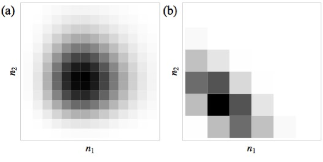
Figure 8: Two-photon-number probability density for (a) the harmonic oscillator case with $z=3.5$ and (b) the case $\mu=5$ with $z=10^{5}.$

The linear entropy for our coherent state on a beamsplitter will be (see Hoffmann2018c )

$$S(|z|)=1-\sum_{r_{1}=0}^{\infty}\sum_{r_{2}=0}^{\infty}|M(r_{1},r_{2};z)|^{2}.$$ (III.17)

with

$$M(r_{1},r_{2};z)=\sum_{\kappa=0}^{\infty}G(\kappa+r_{1},r_{1};z)G^{*}(\kappa+r_{2},r_{2};z).$$ (III.18)

and

$$G(k,r;z) =\alpha_{k}^{(5)}(z)\frac{1}{2^{\frac{k}{2}}}\binom{k}{r}^{\frac{1}{2}}=\frac{1}{\sqrt{F^{(5)}(z)}}\frac{z^{k}}{D_{k}^{(5)}}\frac{1}{2^{\frac{k}{2}}}\binom{k}{r}^{\frac{1}{2}}.$$ (III.19)

We take the sums to $\kappa=10$ and $r_{1}=r_{2}=10.$

We plot the linear entropy to $|z|=10^{5}$ in Figure 9. We see that it remains small, indicating a low degree of entanglement.

Figure 9: Linear entropy for $\mu=5$ on a beamsplitter.

III.6 Heisenberg uncertainty principle

We use results from Hoffmann2018c (with $\alpha_{k}=\alpha_{k}^{(5)}(z)$)

$$\langle\,z\,|\,\hat{x}\,|\,z\,\rangle = \sum_{k_{1}=0}^{\infty}\sum_{k_{2}=0}^{\infty}\alpha_{k_{1}}^{*}M_{k_{1}k_{2}}^{(x)}\alpha_{k_{2}},$$

$$\langle\,z\,|\,\hat{x}^{2}\,|\,z\,\rangle = \sum_{k_{1}=0}^{\infty}\sum_{k_{2}=0}^{\infty}\alpha_{k_{1}}^{*}M_{k_{1}k_{2}}^{(x^{2})}\alpha_{k_{2}},$$

$$\langle\,z\,|\,\hat{p}\,|\,z\,\rangle = \sum_{k_{1}=0}^{\infty}\sum_{k_{2}=0}^{\infty}\alpha_{k_{1}}^{*}M_{k_{1}k_{2}}^{(p)}\alpha_{k_{2}},$$

$$\langle\,z\,|\,\hat{p}^{2}\,|\,z\,\rangle = \sum_{k_{1}=0}^{\infty}\sum_{k_{2}=0}^{\infty}\alpha_{k_{1}}^{*}M_{k_{1}k_{2}}^{(p^{2})}\alpha_{k_{2}},$$ (III.20)

with

$$M_{k_{1}k_{2}}^{(x)} = \int_{0}^{\infty}dx\,\langle\,5+6k_{1}\,|\,x\,\rangle x\langle\,x\,|\,5+6k_{2}\,\rangle,$$

$$M_{k_{1}k_{2}}^{(x^{2})} = \int_{0}^{\infty}dx\,\langle\,5+6k_{1}\,|\,x\,\rangle x^{2}\langle\,x\,|\,5+6k_{2}\,\rangle,$$

$$M_{k_{1}k_{2}}^{(p)} = \int_{0}^{\infty}dx\,\langle\,5+6k_{1}\,|\,x\,\rangle(-i\frac{d}{dx})\langle\,x\,|\,5+6k_{2}\,\rangle,$$

$$M_{k_{1}k_{2}}^{(p^{2})} = \int_{0}^{\infty}dx\,\langle\,5+6k_{1}\,|\,x\,\rangle(-\frac{d^{2}}{dx^{2}})\langle\,x\,|\,5+6k_{2}\,\rangle,$$ (III.21)

all integrated only on the right half-plane. With the range of $|z|$ considered, we may cut off the sums at $k_{1}=k_{2}=6$ with negligible error. Once these expectations are calculated, we use

$$\sigma_{x} =\sqrt{\langle\,x^{2}\,\rangle-\langle\,x\,\rangle^{2}},$$

$$\sigma_{p} =\sqrt{\langle\,p^{2}\,\rangle-\langle\,p\,\rangle^{2}}.$$ (III.22)

The functions $\sigma_{x}(z)$ and $\sigma_{p}(z)$ and their product are plotted in Figure 10 for real values of $z.$ We see no squeezing in this regime, as the standard deviations remain larger than $1/\sqrt{2}$. The product $\sigma_{x}\sigma_{p}$ remains greater than $1/2.$

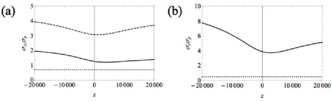
Figure 10: The spreads $\sigma_{x}(z)$ (solid) and $\sigma_{p}(z)$ (dashed) are plotted in (a), compared to $1/\sqrt{2}$ (dotted) for real $z$. Their product is plotted in (b) for real $z$ (solid) compared to $1/2$ (dotted).

III.7 Number statistics: Mandel $Q$ parameter

As in Hoffmann2018c , we define a number of excitations operator by

$$N\,|\,5+6k\,\rangle=k\,|\,5+6k\,\rangle.$$ (III.23)

The Mandel $Q$ parameter, defined by

$$Q=\frac{\Delta N^{2}-\langle\,N\,\rangle}{\langle\,N\,\rangle}=\frac{\langle\,N^{2}\,\rangle-\langle\,N\,\rangle^{2}-\langle\,N\,\rangle}{\langle\,N\,\rangle},$$ (III.24)

is zero for Poissonian statistics, positive for super-Poissonian statistics and negative for sub-Poissonian statistics.

We calculate the expectations by

$$\langle\,N\,\rangle =\sum_{k=0}^{\infty}|\alpha_{k}^{(5)}(z)|^{2}\,k,$$

$$\langle\,N^{2}\,\rangle =\sum_{k=0}^{\infty}|\alpha_{k}^{(5)}(z)|^{2}\,k^{2}.$$ (III.25)

The results are plotted in Figure 11, showing Poissonian statistics only for $z=0$ and sub-Poissonian statistics for greater values of $|z|.$

Figure 11: Mandel $Q$ parameter for $\mu=5.$

IV Comparison with other work

Fernández C. et al. Fernandez2018b considered the same 4-step construction, with the choices in Eq. (II.31), that we have used in this paper. They constructed coherent states for linear ladder operators defined by

$$\mathcal{L}^{-}\,|\,\nu\,\rangle=\sqrt{\nu-1}\,|\,\nu-2\,\rangle,\quad\mathcal{L}^{+}\,|\,\nu\,\rangle=\sqrt{\nu+1}\,|\,\nu+2\,\rangle,\quad\mathrm{for}\ \nu=1,3,\dots,$$ (IV.1)

when acting only on the part of the spectrum isospectral with the truncated harmonic oscillator. Since they lower or raise the index by 2, they can be considered linearized versions of our ladder operators $\tilde{L}$ and $\tilde{L}^{\dagger},$ respectively. These authors use the displacement operator to define their coherent states, but since the structure is just that of the harmonic oscillator, this gives the same result as the Barut-Girardello definition Barut1971 . Of course it is the fact that the position wavefunctions differ from those of the harmonic oscillator that leads to new and interesting results.

These authors find squeezing in $p,$ whereas we found no squeezing for real $z.$ For their coherent state on one arm of a beamsplitter, they found a linear entropy that was largely flat as a function of $|z|,$ with values close to $0.5,$ whereas we found a function at first decreasing, then flat, close to 0.2 asymptotically. Thus the degree of entanglement was low for both cases. Our variation was over a much larger scale of $|z|,$ understood from the presence of large denominators, as explained for energy expectations in Section III A.

Two coherent states of completely different construction, as we have here, are not expected to have similar physical properties at equal $z$ values. Instead, the energy expectation allows a more meaningful comparison. The energy expectation for the coherent states constructed by Fernández C. et al. Fernandez2018b would be

$$E_{F}(|z|)=3+2|z|^{2}.$$

They consider $|z|$ values as large as 3, giving a maximum energy of 21. This, from Figure 3, is comparable to the energies we were considering.

We did not expect close agreement with Fernández C. et al. Fernandez2018b , as the structure of the coherent states differed (our ladder operators change the index by 6 rather than 2) and the coefficients in the superpositions are distinctly different.

V Conclusions

We constructed the coherent states that are eigenvectors of the $\tilde{C}$ ladder operator with complex eigenvalue $z$ and lowest weight $\mu=5.$

The energy expectation was found to vary slowly with $|z|.$ Thus we chose to consider coherent states for the other tests with $z$ values sufficiently large to make the energy expectation sufficiently different from the ground state energy. We plotted the time-dependent position probability density over one period for $z=10^{5}$ and found a great deal of structure. Such was also the case for the even and odd cat state densities.

The Wigner function for $z=500$ displayed a great deal of structure and showed no definitive regions of negative value. So we could not claim to have seen the signature of nonclassical behaviour.

For the coherent states on one arm of a beamsplitter, the two “photon” probability distribution was seen to not factorize and was plotted for $z=10^{5}.$ The linear entropy was found to be significantly low compared to unity up to $z=10^{5},$ indicating a low degree of entanglement.

Calculation of the standard deviations in position and momentum for real $z$ with $|z|\leq 20\,000$ showed no squeezing. The Heisenberg uncertainty principle was satisfied as a check on our calculations.

Calculation of the Mandel $Q$ parameter showed the number statistics of our coherent states to be sub-Poissonian up to $z=10^{5},$ Poissonian only for $z=0.$

We conclude that the majority of these indicators suggested non-classical behaviour for these coherent states.

We compared our results with those of Fernández C. et al. Fernandez2018b for the same basis states and position wavefunctions but quite different coherent states. As expected, our results differed from theirs.

- (1) Witten E. Dynamical breaking of supersymmetry. Nucl Phys B. 1981;188:513.
- (2) Witten E. Constraints on supersymmetry breaking. Nucl Phys B. 1982;202:253.
- (3) Mielnik B. Factorization method and new potentials with the oscillator spectrum. J Math Phys. 1984;25:3387.
- (4) Andrianov AA, Ioffe MV, Spiridonov VP. Higher-derivative supersymmetry and the Witten index. Phys Lett A. 1993;174:273.
- (5) Andrianov AA, Ioffe MV, Cannata F, Dedonder JP. Second order derivative supersymmetry, q deformations and the scattering problem. Int J Mod Phys A. 1995;10:2683.
- (6) Cooper F, Khare A, Sukhatme U. Supersymmetry and quantum mechanics. Phys Rep. 1995;251:267.
- (7) Fernández C DJ, Glasser ML, Nieto LM. New isospectral oscillator potentials. Phys Lett A. 1998;240:15.
- (8) Fernández C DJ, Hussin V, Mielnik B. A simple generation of exactly solvable anharmonic oscillators. Phys Lett A. 1998;244:309.
- (9) Samsonov BF. New possibilities for supersymmetry breakdown in quantum mechanics and second-order irreducible Darboux transformations. Phys Lett A. 1999;263:274.
- (10) Mielnik B, Nieto LM, Rosas-Ortiz O. The finite difference algorithm for higher order supersymmetry. Phys Lett A. 2000;269:70.
- (11) Cariñena JF, Ramos A, Fernández C DJ. Group theoretical approach to the intertwined Hamiltonians. Ann Phys (NY). 2001;292:42.
- (12) Aoyama H, Sato M, Tanaka T. N-fold supersymmetry in quantum mechanics: general formalism. Nucl Phys B. 2001;619:105.
- (13) Carballo JM, Fernández C DJ, Negro J, Nieto LM. Polynomial Heisenberg algebras. J Phys A Math Gen. 2004;37:10349.
- (14) Marquette I. Superintegrability with third order integrals of motion, cubic algebras, and supersymmetric quantum mechanics. II. Painlevé transcendent potentials. J Math Phys. 2009;50:095202.
- (15) Fernández C DJ. Supersymmetric Quantum Mechanics. In: Garcia Rocha M, Lopez Fernandez R, Rojas Ochoa LF, Torres Vega G, editors. AIP Conf. Ser.. vol. 1287; 2010. p. 3.
- (16) Quesne C. Higher-order SUSY, exactly solvable potentials, and exceptional orthogonal polynomials. Mod Phys Lett A. 2011;26:1843.
- (17) Marquette I. Classical ladder operators, polynomial Poisson algebras, and classification of superintegrable systems. J Math Phys. 2012;53:012901.
- (18) D Gómez-Ullate YG, Milson R. Rational extensions of the quantum harmonic oscillator and exceptional Hermite polynomials. J Phys A: Math Theor. 2014;47:015203.
- (19) Marquette I, Quesne C. Combined state-adding and state-deleting approaches to type III multi-step rationally extended potentials: Applications to ladder operators and superintegrability. J Math Phys. 2014;55:112103.
- (20) Fernández C DJ, Morales-Salgado VS. Supersymmetric partners of the harmonic oscillator with an infinite potential barrier. J Phys A Math Gen. 2014;47:035304.
- (21) Fernández C DJ, Morales-Salgado VS. SUSY partners of the truncated oscillator, Painlevé transcendents and Bäcklund transformations. J Phys A Math Gen. 2016;49:195202.
- (22) Fernandez C DJ, Hussin V, Morales-Salgado V. Coherent states for the supersymmetric partners of the truncated oscillator. arXiv:170808010v2, to be published in EPJ Plus. 2018;.
- (23) Márquez IF, Negro J, Nieto LM. Factorization method and singular Hamiltonians. J Phys A Math Gen. 1998;31:4115.
- (24) Glauber RJ. The quantum theory of optical coherence. Phys Rev. 1963;130:2529.
- (25) Glauber RJ. Coherent and incoherent states of the radiation field. Phys Rev. 1963;131:2766.
- (26) Klauder JR. Continuous representation theory. I. Postulates of continuous representation theory. J Math Phys. 1963;4:1055.
- (27) Klauder JR. Continuous representation theory. II. Generalized relation between quantum and classical dynamics. J Math Phys. 1963;4:1058.
- (28) Barut AO, Girardello L. New ”coherent” states associated with non compact groups. Commun Math Phys. 1971;21:41.
- (29) Perelomov A. Generalized coherent states and their applications. Springer-Verlag, Berlin, Heidelberg; 1986.
- (30) Gazeau JP, Klauder JR. Coherent states for systems with discrete and continuous spectrum. J Phys A: Math Gen. 1999;32:123.
- (31) Quesne C. Generalized coherent states associated with the Cv-extended oscillator. Ann Phys (NY). 2001;293:147.
- (32) Fernández DJ, Nieto LM, Rosas-Ortiz O. Distorted Heisenberg algebra and coherent states for isospectral oscillator Hamiltonians. J Phys A: Math Gen. 1995;28:2693.
- (33) Fernández DJ, Hussin V. Higher-order SUSY, linearized nonlinear Heisenberg algebras and coherent states. J Phys A: Math Gen. 1999;32:3603.
- (34) Ali ST, Antoine JP, Gazeau JP. Coherent states, wavelets and their generalizations. 2nd ed. Springer-Verlag, New York; 2014.
- (35) Gradsteyn IS, Ryzhik IM. Tables of Integrals, Series and Products. Corrected and enlarged ed. Academic Press, Inc., San Diego, CA; 1980.
- (36) Fernández C DJ, Morales-Salgado VS. Higher order supersymmetric truncated oscillators. Ann Phys (NY). 2018 Jan;388:122–134.
- (37) Hoffmann SE, Hussin V, Marquette I, Zhang YZ. Coherent states for ladder operators of general order related to exceptional orthogonal polynomials. J Phys A: Math Theor. 2018;51:315203.