Structured Pruning of Neural Networks with Budget-Aware Regularization

Abstract

Pruning methods have shown to be effective at reducing the size of deep neural networks while keeping accuracy almost intact. Among the most effective methods are those that prune a network while training it with a sparsity prior loss and learnable dropout parameters. A shortcoming of these approaches however is that neither the size nor the inference speed of the pruned network can be controlled directly; yet this is a key feature for targeting deployment of CNNs on low-power hardware. To overcome this, we introduce a budgeted regularized pruning framework for deep CNNs. Our approach naturally fits into traditional neural network training as it consists of a learnable masking layer, a novel budget-aware objective function, and the use of knowledge distillation. We also provide insights on how to prune a residual network and how this can lead to new architectures. Experimental results reveal that CNNs pruned with our method are more accurate and less compute-hungry than state-of-the-art methods. Also, our approach is more effective at preventing accuracy collapse in case of severe pruning; this allows pruning factors of up to $16\times$ without significant accuracy drop.

1 Introduction

Convolutional Neural Networks (CNN) have proven to be effective feature extractors for many computer vision tasks [12, 15, 18, 30]. The design of several CNNs involve many heuristics, such as using increasing powers of two as the number of feature maps, or width, of each layer. While such heuristics allow achieving excellent results, they may be too crude in situations where the amount of compute power and memory is restricted, such as with mobile platforms. Thus arises the problem of finding the right number of layers that solve a given task while respecting a budget. Since the number of layers depends highly on the effectiveness of the learned filters (and their combination), one cannot determine these hyper-parameters a priori.

Convolution operations constitute the main computational burden of a CNN. The execution of these operations benefit from a high degree of parallelism, which requires them to have regular structures. This implies that one cannot remove isolated neurons from a CNN filter as they must be full grids. To achieve the same effect as removing a neuron, one can zero-out its weights. While doing this reduces the theoretical size of the model, it does not reduce the computational demands of the model nor the amount of feature map memory. Therefore, to accelerate a CNN and reduce its memory footprint, one has to rely on structured sparsity pruning methods that aim at reducing the number of feature maps and not just individual neurons.

By removing unimportant filters from a network and retraining it, one can shrink it while maintaining good performance [10, 19]. This can be explained by the following hypothesis: the initial value of a filter’s weights is not guaranteed to allow the learning of a useful feature; thus, a trained network might contain many expendable features [7].

Among the structured pruning methods, those that implement a sparsity learning (SL) framework have shown to be effective as pruning and training are done simultaneously [4, 17, 21, 22, 24, 26]. Unfortunately, most SL methods cannot prune a network while respecting a neuron budget imposed by the very nature of a device on which the network shall be deployed. As of today, pruning a network while respecting a budget can only be done by trial-and-error, typically by training multiple times a network with various pruning hyperparameters.

In this paper, we present a SL framework which allows learning and selecting filters of a CNN while respecting a neuron budget. Our main contributions are:

• We present a novel objective function which includes a variant of the log-barrier [1] function for simultaneously training and pruning a CNN while respecting a total neuron budget;

• We propose a variant of the barrier method [1] for optimizing a CNN;

• We demonstrate the effectiveness of combining SL and knowledge distillation [14];

• We empirically confirm the existence of the automatic depth determination property of residual networks pruned with filter-wise methods, and give insights on how to ensure the viability of the pruned network by preventing “fatal pruning”;

• We propose a new mixed-connectivity block which roughly doubles the effective pruning factors attainable with our method.

2 Previous Works

Compressing neural networks without affecting too much their accuracy implies that networks are often over-parametrized. Denil et al. [5] have shown that typical neural networks are over-parametrized; in the best case of their experiments, they could predict 95% of the network weights from the others. Recent work by Frankle et al. [7] support the hypothesis that a large proportion (typically 90%) of weights in standard neural networks are initialized to a value that will lead to an expendable feature. In this section, we review six categories of methods for reducing the size of a neural network.

Neural network compression aims to reduce the storage requirements of the network’s weights. In [6, 16], low-rank approximation through matrix factorization, such as singular-value decomposition, is used to factorize the weight matrices. The factors’ rank is reduced by keeping only the leading eigenvalues and their associated eigenvectors. In [8], quantization is used to reduce the storage taken by the model; both scalar quantization and vector quantization (VQ) have been considered. Using VQ, a weight matrix can be reconstructed from a list of indices and a dictionary of vectors. Thus, practical computation savings can be obtained. Unfortunately, most network compression methods do not decrease the memory and compute usage during inference.

Neural network pruning consists of identifying and removing neurons that are not necessary for achieving high performance. Some of the first approaches used the second-order derivative to determine the sensitivity of the network to the value of each weight [19, 11]. A more recent, very simple and effective approach selects which neurons to remove by thresholding the magnitude of their weights; smaller magnitudes are associated with unimportant neurons [10]. The resulting network is then finetuned for better performance. Nonetheless, experimental results (c.f. [sec:experiments]Section 5) show that variational pruning methods (discussed below) outperform the previously mentioned works.

Sparsity Learning (SL) methods aim at pruning a network while training it. Some methods add to the training loss a regularization function such as $L_{1}$ [21], Group LASSO [33], or an approximation of the $L_{0}$ norm [22, 27]. Several variational methods have also been proposed [4, 17, 26, 24]. These methods formalize the problem of network pruning as a problem of learning the parameters of a dropout probability density function (PDF) via the reparametrization trick [17]. Pruning is enforced via a sparsity prior that derives from a variational evidence lower bound (ELBO). In general, SL methods do not apply an explicit constraint to limit the number of neurons used. To enforce a budget, one has to turn towards budgeted pruning.

Budgeted pruning is an approach that provides a direct control on the size of the pruned network via some “network size” hyper-parameter. MorphNet [9] alternates between training with a $L_{1}$ sparsifying regularizer and applying a width multiplier to the layer widths to enforce the budget. Contrary to our method, this work does not leverage dropout-based SL. Budgeted Super Networks [32] is a method that finds an architecture satisfying a resource budget by sparsifying a super network at the module level. This method is less convenient to use than ours, as it requires “neural fabric” training through reinforcement learning. Another budgeted pruning approach is “Learning-Compression” [3], which uses the method of auxiliary coordinates [2] instead of back-propagation. Contrary to this method, our approach adopts a usual gradient descent optimization scheme, and does not rely on the magnitude of the weights as a surrogate of their importance.

Architecture search (AS) is an approach that led to efficient neural networks in terms of performance and parameterization. Using reinforcement learning and vast amounts of processing power, NAS [35] have learned novel architectures; some that advanced the state-of-the-art, others that had relatively few parameters compared to similarly effective hand-crafted models. PNAS [20] and ENAS [29] have extended this work by cutting the necessary compute resources. These works have been aggregated by EPNAS [28]. AS is orthogonal to our line of work as the learned architectures could be pruned by our method. In addition, AS is more complicated to implement as it requires learning a controller model by reinforcement learning. In contrast, our method features tools widely used in CNN training.

3 Our Approach

3.1 Dropout Sparsity Learning

Before we introduce the specifics of our approach, let us first summarize the fundamental concepts of Dropout Sparsity Learning (DSL).

Let $\mathbf{h}_{l}$ be the output of the $l$-th hidden layer of a CNN computed by $f_{l}(\mathbf{h}_{l-1})$, a transformation of the previous layer, typically a convolution followed by a batch norm and a non-linearity. As mentioned before, one way of reducing the size of a network is by shutting down neurons with an element-wise product $\odot$ between the output of layer $\mathbf{h}_{l-1}$ and a binary tensor $\mathbf{z}_{l-1}$:

$$\mathbf{h}_{l}=f_{l}(\mathbf{h}_{l-1}\odot\mathbf{z}_{l-1}).$$ (1)

To enforce structured pruning and shutdown feature maps (not just individual neurons), one can redefine $\mathbf{z}_{l-1}$ as a vector of size $d_{l-1}$ where $d_{l-1}$ is the number of feature maps in $\mathbf{h}_{l-1}$. Then, $\mathbf{z}_{l-1}$ is applied over the spatial dimensions by performing an element-wise product with $\mathbf{h}_{l-1}$.

As one might notice, [eq:dropout]Eq. (1) is the same as that of dropout [31] for which $\mathbf{z}_{l-1}$ is a tensor of independent random variables i.i.d. of a Bernoulli distribution $q(z)$. To prune a network, DSL redefines $\mathbf{z}_{l-1}$ as random variables sampled from a distribution $q(z|\Phi)$ whose parameters $\Phi$ can be learned while training the model. In this way, the network can learn which feature maps to drop and which ones to keep.

Since the operation of sampling $\mathbf{z}_{l-1}$ from a distribution is not differentiable, it is common practice to redefine it with the reparametrization trick [17]:

$$\mathbf{h}_{l}=f_{l}(\mathbf{h}_{l-1}\odot g(\Phi_{l-1},\epsilon))$$ (2)

where $g$ is a continuous function differentiable with respect to $\Phi$ and stochastic with respect to $\epsilon$, a random variable typically sampled from $\mathcal{N}(0,1)$ or $\mathcal{U}(0,1)$.

In order to enforce network pruning, one usually incorporates a two-term loss :

$$L(W,\Phi)=L_{D}(W,\Phi)+\lambda L_{S}(\Phi)$$ (3)

where $\lambda$ is the prior’s weight, $W$ are the parameters of the network, $L_{D}(W,\Phi)$ is a data loss that measures how well the model fits the training data (e.g. the cross-entropy loss) and $L_{S}$ is a sparsity loss that measures how sparse the model is. While $L_{S}$ varies from one method to another, the KL divergence between $q(z|\Phi)$ and some prior distribution is typically used by variational approaches [17, 24]. Note that during inference, one can make the network deterministic by replacing the random variable $\epsilon$ by its mean.

3.2 Soft and hard pruning

As mentioned before, $g(\Phi_{l-1},\epsilon)$ is a continuous function differentiable with respect to $\Phi_{l-1}$. Thus, instead of being binary, the pruning of [eq:dropout2]Eq. (2) becomes continuous (soft pruning), so there is always a non-zero probability that a feature map will be activated during training. However, to achieve practical speedups, one eventually needs to “hard-prune” filters. To do so, once training is over, the values of $\Phi$ are thresholded to select which filters to remove completely. Then, the network may be fine-tuned for several epochs with the $L_{D}$ loss only, to let the network adapt to hard-pruning. We call this the “fine-tuning phase”, and the earlier epochs constitute the “training phase”.

3.3 Budget-Aware Regularization (BAR)

In our implementation, a budget is the maximum number of neurons a “hard-pruned” network is allowed to have. To compute this metric, one may replace $z\sim q(z|\Phi)$ by its mean so feature maps with $\mathbb{E}[z|\Phi]=0$ have no effect and can be removed, while the others are kept. The network size is thus the total activation volume of the structurally “hard-pruned” network :

$$V=\sum_{l}\sum_{i}\mathds{1}(\mathbb{E}[z_{l,i}|\Phi]>0)\times A_{l}$$ (4)

where $A_{l}$ is the area of the output feature maps of layer $l$ and $\mathds{1}$ is the indicator function. Our training process is described in Algorithm 1.

Data: $W$: network weights; $\Phi$: r.v. parametrization; TeacherLogits: the class-wise scores for all samples of the dataset; $\boldsymbol{\lambda}$: all the hyperparameters of the method (including the budget); Prog $\in[0,1]$: progress of the training process; $g(\cdot)$: function introduced in Eq. (2) of the paper; $\mathbf{\hat{y}}$: predicted class-wise logits.

Result: PrunedNet: the pruned neural network object including its weights.

1

2$W^{\prime}\Leftarrow$ TrainUnprunedNetwork()

3 TeacherLogits $\Leftarrow$ PredictWholeDataset($W^{\prime}$)

4 for $b\in\mbox{Minibatches}$ do

5       $(\mathbf{x},\mathbf{y})\Leftarrow b$

6       $\mathbf{z}\Leftarrow g(\Phi,\boldsymbol{\epsilon}),\boldsymbol{\epsilon}\sim\mathcal{U}(0,1)$

7       $\mathbf{\hat{y}}\Leftarrow$ ForwardPass($\mathbf{x},W,\mathbf{z}$)

8       $l\Leftarrow$ BARLoss($\mathbf{y},\mathbf{\hat{y}},\mathbf{z},\boldsymbol{\lambda},\mbox{TeacherLogits},\textnormal{{Prog}}$)

9       $(\nabla W,\nabla\Phi)\Leftarrow$ BackwardPass($l$)

10       $(W,\Phi)\Leftarrow$ OptimizationStep($\nabla W,\nabla\Phi$)

11      

12PruningMasks $\Leftarrow g(\Phi,\mathbb{E}[\epsilon])$

13 PrunedNet $\Leftarrow$ ConvertNet($W$, PruningMasks)

Algorithm 1 BAR Training

A budget constraint imposes on $V$ to be smaller than the allowed budget $b$. If embedded in a sparsity loss, that constraint makes the loss go to infinity when $V>b$, and zero otherwise. This is a typical inequality constrained minimization problem whose binary (and yet non-differentiable) behavior is not suited to gradient descent optimization. One typical solution to such problem is the log-barrier method [1]. The idea of this barrier method is to approximate the zero-to-infinity constraint by a differentiable logarithmic function : $-(1/t)\log(b-V)$ where $t>0$ is a parameter that adjusts the accuracy of the approximation and whose value increases at each optimization iteration (c.f. Algo 11.1 in [1]).

Unfortunately, the log-barrier method requires beginning optimization with a feasible solution (i.e. $V<b$), and this brings two major problems. First, we need to compute $\Phi$ such that $V<b$, which is no trivial task. Second, this induces a setting similar to training an ensemble of pruned networks, as the probability that a feature map is “turned on” is very low. This means that filters will receive little gradient and will train very slowly. To avoid this, we need to start training with a $V$ larger than the budget.

We thus implemented a modified version of the barrier algorithm. First, as will be shown in the rest of this section, we propose a barrier function $f(V,a,b)$ as a replacement for the log barrier function (c.f. [fig:barrier]Fig. 1). Second, instead of having a fixed budget $b$ and a parameter $t$ that grows at each iteration as required by the barrier method, we eliminate the hardness parameter $t$ and instead decrease the budget constraint at each iteration. This budget updating schedule is discussed in [pruningtargettrans]Section 3.4.

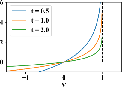
(a) Logarithmic barrier function

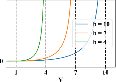
(b) Our barrier function

Figure 1: Comparing barrier functions. (a) Common barrier function $-(1/t)\log(b-V)$ with $b=1$. (b) Our barrier function $f(V,a,b)$ with $a=1$.

Our barrier function $f(V,a,b)$ is designed such that:

• it has an infinite value when the volume used by a network exceeds the budget, i.e. $V>b$;

• it has a value of zero when the budget is comfortably respected, i.e. $V<a$;

• it has $C^{1}$ continuity.

Instead of having a jump from zero to infinity at the point where $V>b$, we define a range where a smooth transition occurs. To do so, we first perform a linear mapping of $V$ :

$$c=\frac{V-a}{b-a}$$

such that $V=a\Rightarrow c=0$ (the budget is comfortably respected), and $V=b\Rightarrow c=1$ (our constraint $V<b$ is violated). Then, we use the following function:

$$g(c)=\frac{c^{2}}{1-c}$$

which has three useful properties: ($i$) $g(0)=0$ and $g(0)^{\prime}=0$, ($ii$) $\lim_{c\to 1^{-}}g(c)=\infty$ and ($iii$) it has a $C^{1}$ continuity. Those properties correspond to the ones mentioned before. To obtain the desired function, we substitute $c$ in $g(c)$ and simplify:

$$f(V,a,b)=\begin{cases}0&V\leq a\\ \frac{(V-a)^{2}}{(b-V)(b-a)}&a<V<b\\ \infty&V\geq b.\end{cases}$$ (5)

As shown in [fig:barrier]Fig. 1, like for log barrier, $V=b$ is an asymptote, as we require $V<b$. However, $a<V<b$ corresponds to a respected budget and for $V\leq a$, the budget is respected with a comfortable margin, and this corresponds to a penalty of zero.

Our proposed prior loss is as follows:

$$L_{\text{BAR}}(\Phi,V,a,b)=L_{S}(\Phi)f(V,a,b)$$ (6)

where $(a,b)$ are the lower and upper budget margins, $V$ is the current “hard-pruned” volume as computed by [eq:omega]Eq. (4), and $L_{S}(\Phi)$ is a differentiable approximation of $V$. Note that since $V$ is not differentiable w.r.t to $\Phi$, we cannot solely optimize $f(V,a,b)$.

The content of $L_{S}(\Phi)$ is bound to $q(z|\Phi)$. In our case, we use the Hard-Concrete distribution (which is a smoothed version of the Bernoulli distribution), as well as its corresponding prior loss, both introduced in [22]. This prior loss measures the expectation of the number of feature maps currently unpruned. To account for the spatial dimensions of the output tensors of convolutions, we use:

$$L_{S}(\Phi)=\sum_{l}L_{S}(\Phi_{l})=\sum_{l}L_{HC}(\Phi_{l})\times A_{l}$$

where $L_{HC}$ is the hard-concrete prior loss [22] and $A_{l}$ is the area of the output feature maps of layer $l$. Thus, $L_{S}(\Phi)$ measures the expectation of the activation volume of all convolution operations in the network.

Note that $V$ could also be replaced by another metric, such as the total FLOPs used by the network. In this case, $L_{S}(\Phi_{l})$ should also include the expectation of the number of feature maps of the preceding layer.

3.4 Setting the budget margins $(a,b)$

As mentioned earlier, initializing the network with a volume that respects the budget (as required by the barrier method) leads to severe optimization issues. Instead, we iteratively shift the pruning target $b$ during training. Specifically, we shift it from $b=V_{F}$ at the beginning, to $b=B$ at the end (where $V_{F}$ is the unpruned network’s volume and $B$ the maximum allowed budget).

As shown in [fig:barrier]Fig. 1b, doing so induces a lateral shift to the “barrier”. This is unlike the barrier method in which the hardness parameter $t$ evolves in time (c.f. [fig:barrier]Fig. 1a). Mathematically, the budget $b$ evolves as follows:

$$\begin{split}b&=(1-T(i))\ V_{F}+T(i)\ B,\\ i&=\frac{\mathrm{iteration\ index}}{\mathrm{num.\ training\ iterations}}\end{split}$$ (7)

while $a=B-10^{-4}\ V_{F}$ is fixed. Here $T(i)$ is a transition function which goes from zero at the first iteration all the way to one at the last iteration. While $T(i)$ could be a linear transition schedule, experimental results reveal that when $b$ approaches $B$, some gradients suffers from extreme spikes due to the nature of $f(V,a,b)$. This leads to erratic behavior towards the end of the training phase that can hurt performance. One may also implement an exponential transition schedule. This could compensate for the shape of $f(V,a,b)$ by having $b$ change quickly during the first epochs and slowly towards the end of training. While this gives good results for severe pruning (up to $16\times$), the increased stress at the beginning yields sub-optimal performance for low pruning factors.

For our method, we propose a sigmoidal schedule, where $b$ changes slowly at the beginning and at the end of the training phase, but quickly in the middle. This puts most of the “pruning stress” in the middle of the training phase, which accounts for the difficulty of pruning (1) during the first epochs, where the filters’ relevance is still unknown, and (2) during the last epochs, where more compromises might have to be made. The sigmoidal transition function is illustrated in [fig:sigmoid]Fig. 2 (c.f. Supp. materials for details).

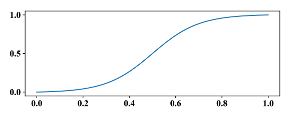
Figure 2: Sigmoidal transition function.

3.5 Knowledge Distillation

Knowledge Distillation (KD) [14] is a method for facilitating the training of a small neural network (the student) by having it reproduce the output of a larger network (the teacher). The loss proposed by Hinton et al [14] is :

$$L_{D}(W)=(1-\alpha)L_{CE}(P_{s},Y_{gt})+\alpha T^{2}L_{CE}(P_{s},P_{t})$$

where $L_{CE}$ is a cross-entropy, $Y_{gt}$ is the groundtruth, $P_{s}$ and $P_{t}$ are the output logits of the student and teacher networks, $\alpha\in[0,1]$, and $T\geq 1$ is a temperature parameter used to smooth the softmax output : $p_{i}=\frac{\exp(z_{i}/T)}{\sum_{j}\exp(z_{j}/T)}$.

In our case, the unpruned network is the teacher and the pruned network is the student. As such, our final loss is:

$$(1-\alpha)L_{CE}(P_{s},Y_{gt})+\alpha T^{2}L_{CE}(P_{s},P_{t})+\lambda L_{\text{BAR}}(\Phi,V,a,b).$$

where $\lambda$, $\alpha$ and $T$ are fixed parameters.

4 Pruning Residual Networks

While our method can prune any CNN, pruning a CNN without residual connections does not affect the connectivity patterns of the architecture, and simply selects the width at each layer [9]. In this paper, we are interested in allowing any feature map of a residual network to be pruned. This pruning regime can reduce the depth of the network, and generally results in architectures with atypical connectivity that require special care in their implementation to obtain maximum efficiency.

4.1 Automatic Depth Determination

We found, as in [9], that filter-wise pruning can successfully prune entire ResBlocks and change the network depth. This effect was named Automatic Depth Determination in [25]. Since a ResBlock computes a delta that is aggregated with the main (residual) signal by addition (c.f. [fig:resblock]Fig. 3a), such block can generally be removed without preventing the flow of signal through the network. This is because the main signal’s identity connections cannot be pruned as they lack prunable filters.

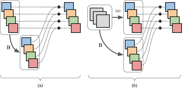
Figure 3: Typical ResBlock vs. pooling block. (a) A typical ResBlock. The “B” arrow is the sequence of convolutions done inside the block. (b) A pooling block at the beginning of a ResNet Layer, that deals with the change in spatial dimensions and number of feature maps. Notice that it breaks the continuity of the residual signal. The arrow labeled “${1}\times{1}$” is a ${1}\times{1}$ convolution with stride 2; the first convolution of “B” also has stride 2. If all convolutions (arrows) are removed, no signal can pass.

However, some ResBlocks, which we call “pooling blocks”, change the spatial dimensions and feature dimensionality of the signal. This type of block breaks the continuity of the residual signal (c.f. [fig:resblock]Fig. 3b). As such, the convolutions inside this block cannot be completely pruned, as this would prevent any signal from flowing through it (a situation we call “fatal pruning”). As a solution, we clamp the highest value of $\Phi$ to ensure that at least one feature map is kept in the ${1}\times{1}$ conv operation.

4.2 Atypical connectivity of pruned ResNets

Our method allows any feature map in the output of a convolution to be pruned (except for the ${1}\times{1}$ conv of the pooling block). This produces three types of atypical residual connectivity that requires special care (see [fig:exotic]Fig. 4). For example, there could be a feature from the residual signal that would pass through without another signal being added to it ([fig:exotic]Fig. 4b). New feature maps can also be created and concatenated ([fig:exotic]Fig. 4c). Furthermore, new feature maps could be created while others could pass through ([fig:exotic]Fig. 4d).

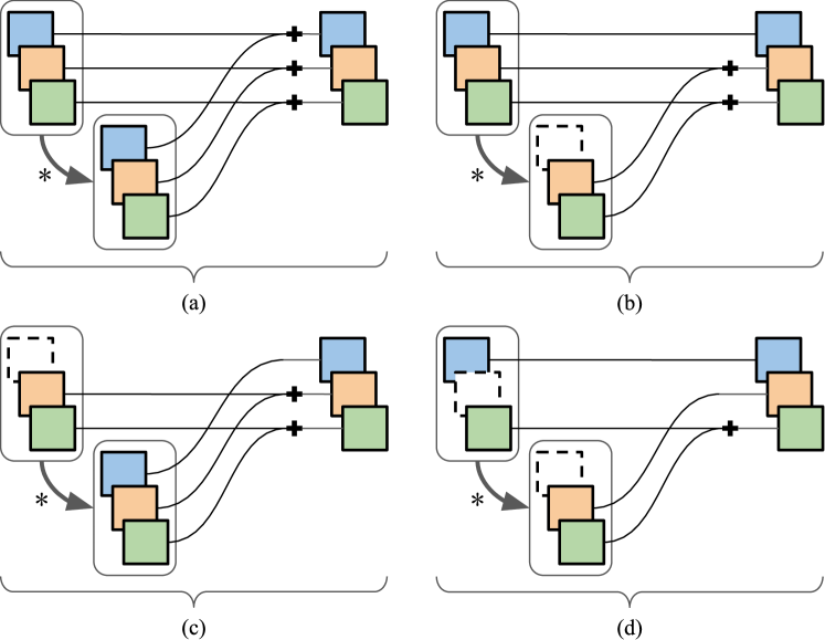
Figure 4: Connectivity allowed by our approach. (a) A 3-feature ResBlock with typical connectivity. Arrows represent one or more convolutions. (b) With one feature map pruned, only two features are computed and added to the residual signal; one feature from the residual signal is left unchanged. (c) a new feature is created and concatenated to the residual signal. (d) a combination of (b) and (c) as a new feature is concatenated to the residual signal, one feature from the residual is left unchanged, and a third feature has typical connectivity (best viewed in color).

To leverage the speedup incurred by a pruned feature map, the three cases in [fig:exotic]Fig. 4 must be taken into account through a mixed-connectivity block which allows these unorthodox configurations. Without this special implementation, some zeroed-out feature maps would still be computed because the summations of residual and refinement signals must have the same number of feature maps. In fact, a naive implementation does not allow refining only a subset of the features of the main signal (as in [fig:exotic]Fig. 4b), nor does it allow having a varying number of features in the main signal (as in [fig:exotic]Fig. 4c).

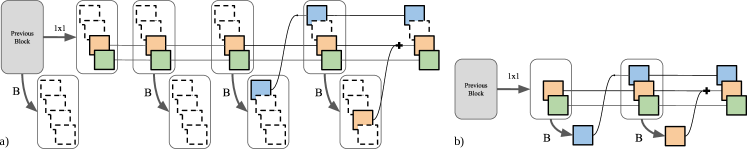
Figure 5: (a) A 4-feature chunk of a ResNet Layer pruned by our method. Dotted feature maps are zeroed-out by their associated mask. An arrow labeled B represents a Block operation, which consist of a sequence of convolutions. Inner convolutions of the Block can be pruned, but only the output of the last convolution is shown (for clarity). (b) The same pruned subgraph, illustrated without the pruned feature maps. The resulting subgraph is shallower and narrower than its “full” counterpart (best viewed in color).

[fig:example]Fig. 5 shows the benefit of a mixed-connectivity block. In (a) is a ResNet Layer pruned by our method. Using a regular ResBlock implementation, all feature maps in pairs of tensors that are summed together need to have matching width. This means that, in [fig:example]Fig. 5, all feature maps of the first, third and fourth rows (features) are computed, even if they are dotted. Only the second row can be fully removed.On the other hand, by using mixed-connectivity, only unpruned feature maps are computed, yielding architectures such as in [fig:example]Fig. 5b, that saves substantial compute (c.f. [sec:experiments]Section 5).

Technical details on our mixed-connectivity block are provided in the Supplementary materials.

5 Experiments

5.1 Experimental Setup

We tested our pruning framework on two residual architectures and report results on four datasets. We pruned Wide-ResNet [34] on CIFAR-10, CIFAR-100 and TinyImageNet (with a width multiplier of 12 as per [34]), and ResNet50 [13] on Mio-TCD [23], a larger and more complex dataset devoted to traffic analysis. TinyImageNet and Mio-TCD samples are resized to ${64}\times{64}$ and ${128}\times{128}$, respectively. Since this ResNet50 has a larger input and is deeper than its CIFAR counterpart, we do not opt for the “wide” version and thus save significant training time. Both network architectures have approximately the same volume.

For all experiments, we use the Adam optimizer with an initial learning rate of $10^{-3}$ and a weight decay of $5\times 10^{-4}$. For CIFAR and TinyImageNet, we use a batch size of 64. For our objective function, we use $\alpha=0.9$, $T=4$, and $\lambda=10^{-5}$. We use PyTorch and its standard image preprocessing. For experiments on Mio-TCD, we start training/pruning with the weights of the unpruned network whereas we initialize with random values for CIFAR and TinyImageNet. Please refer to the Supplementary materials for the number of epochs used in each training phase.

We compare our approach to the following methods:

• Random. This approach randomly selects feature maps to be removed.

• Weight Magnitude (WM) [10]. This method uses the absolute sum of the weights in a filter as a surrogate of its importance. Lower magnitude filters are removed.

• Vector Quantization (VQ) [8] This approach vectorizes the filters and quantizes them into $N$ clusters, where $N$ is the target width for the layer. The clusters’ center are used as the new filters.

• Interpolative Decomposition (ID). This method is based on low-rank approximation for network compression [6, 16]. This algorithm factorizes each filters $W$ into $UV$, where $U$ has a specific number of rows corresponding to the budget. $U$ replaces $W$, and $V$ is multiplied at the next layer (i.e. $W_{l+1}\leftarrow V_{l}W_{l+1}$) to approximate the original sequence of transformations.

• $L_{0}$ regularization (LZR) [22]. This DSL method is the closest to our method. However, it incorporates no budget, penalizes layer width instead of activation tensor volume, and does not use Knowledge Distillation.

• Information Bottleneck (IB) [4]. This DSL method uses a factorized Gaussian distribution (with parameters $\mu,\sigma$) to mask the feature maps as well as the following prior loss : $L_{S}=\log(1-\mu^{2}/\sigma^{2})$.

• MorphNet [9]. This approach uses the $\gamma$ scaling parameter of Batch Norm modules as a learnable mask over features. The said $\gamma$ parameters are driven to zero by a $L_{1}$ objective that considers the resources used by a filter (e.g. FLOPs). This method computes a new width for each layer by counting the non-zero $\gamma$ parameters. We set the sparsity trade-off parameter $\lambda$ after an hyperparameter search, with $16\times$ as the target pruning factor for CIFAR-10.

For every method, we set a budget of tensor activation volume corresponding to $1/2,1/4,1/8,1/16$ of the unpruned volume $V_{F}$. Since LZR and IB do not allow setting a budget, we went through trial-and-error to find the hyperparameter value that yield the desired resource usage. For Random, WM, VQ, and ID we scale the width of all layers uniformly to satisfy the budget and implement a pruning scheme which revealed to be the most effective (c.f. Supplementary materials). We also apply our mixed-connectivity block to the output of every method for a fair comparison.

5.2 Results

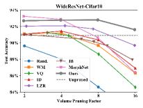
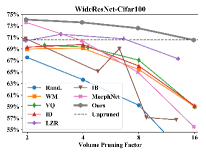
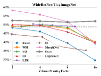
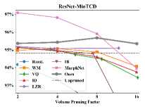
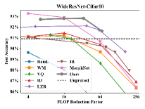
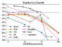
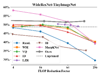
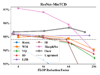
Figure 6: Pruning results. Plots showing test accuracy w.r.t. volume and FLOP reduction factor (best viewed in color).

Results for every method executed on all four datasets are shown in [fig:results_plot]Fig. 6. The first row shows test accuracies w.r.t. the network volume reduction factor for CIFAR-10, CIFAR-100, TinyImageNet and Mio-TCD. As one can see, our method is above the others (or competitive) for CIFAR-10 and CIFAR-100. It is also above every other method on TinyImageNet and Mio-TCD except for MorphNet which is better for pruning factors of 2 and 4. However, MorphNet gets a severe drop of accuracy at 16x, a phenomena we observed as well on CIFAR-10 and CIFAR-100. Our method is also always better than IB and LZR, the other two DSL methods. Overall, our method is resilient to severe (16x) pruning ratios.

Furthermore, for every dataset, networks pruned with our method (as well as some others) get better results than the initial unpruned network. This illustrates the fact that Wide-ResNet and ResNet-50 are overparameterized for certain tasks and that decreasing their number of feature maps reduces overfitting and thus improves test accuracy.

We then took every pruned network and computed their FLOP reduction factor (we considered operations from convolutions only). This is illustrated in the second row of [fig:results_plot]Fig. 6. There again, our method outperforms (or is competitive with) the others for CIFAR-10 and CIFAR-100. Our method reduces FLOPs by up to a factor of $\sim\!64$x on CIFAR-10, $\sim\!60$x on CIFAR-100 and $\sim\!200$x on Mio-TCD without decreasing test accuracy. We get similar results as LZR for pruning ratios around $60$x on CIFAR-10 and CIFAR-100 and $200$x on Mio-TCD. MorphNet gets better accuracy for pruning ratios of $4$x and $16$x on Mio-TCD, but then drops significantly around $256$x. Results are similar for TinyImageNet.

In [tab:ablation]Table 1, we report results of an ablation study on WideResNet-CIFAR-10 with two pruning factors. We replaced the Knowledge Distillation data loss (c.f. [kds]Section 3.5) by a cross-entropy loss, and changed the Sigmoid pruning schedule (c.f. [pruningtargettrans]Section 3.4) by a linear one. As can be seen, removing either of those reduces accuracy, thus showing their efficiency. We also studied the impact of not using the mixed-connectivity block introduced in [atypical]Section 4.2. As shown in [tab:mixtConnBl]Table 2, when replacing our mixed-connectivity blocks by regular ResBlocks, we get a drop of the effective pruned volume of more than 50% for 16x (even up to 58% for CIFAR-10).

Table 1: Test Accuracy for different configurations of our method (using WideResNet-CIFAR-10). The test accuracy of the unpruned network is $90.90\%$.

Configuration	Pruning factor
	2x	16x
Our method	92.70%	91.62%
w/o Knowledge Distillation	-1.37%	-0.40%
w/o Sigmoid pruning schedule	-0.87%	-0.92%

Table 2: Reduction of the effective pruned volume when removing the mixed-connectivity block.

Dataset	2x	4x	8x	16x
CIFAR-10	12%	43%	53%	58%
CIFAR-100	14%	49%	55%	57%
MIO-TCD	32%	37%	40%	52%

We illustrate in [fig:layerpruning]Fig. 7 results of our pruning method for CIFAR-10 (for the other datasets, see supplementary materials). The figure shows the number of neurons per residual block for the full network, and for the networks pruned with varying pruning factors. These plots show that our method has the capability of eliminating entire residual blocks (especially around 1.3 and 1.4). Also, the pruning configurations follow no obvious trend thus showing the inherent plasticity of a DSL method such as ours.

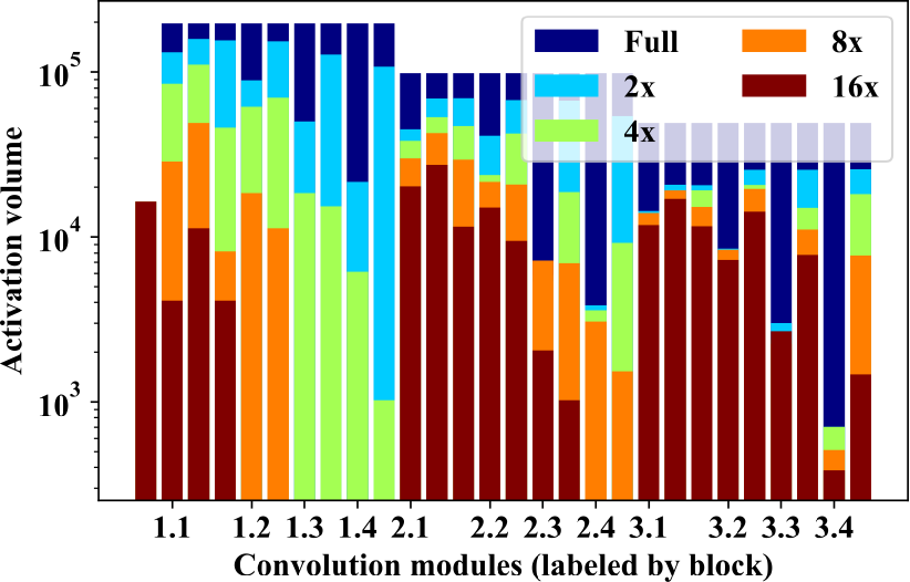
Figure 7: Result of pruning with our method on WideResNet-CIFAR-10. Total number of active neurons in the full networks and with four different pruning rates. Sections without an orange (8x) or red (16x) bar are those for which a res-Block has been eliminated.

As mentioned in [bar]Section 3.3, instead of the volume metric ([eq:omega]Eq. (4)) the budget could be set w.r.t a FLOP metric by accounting for the expectation of the number of feature maps in the preceding layer. We compare in [fig:vftrained]Fig. 8 the results given by these two budget metrics for WideResnet-CIFAR-10. As one might expect, pruning a network with a volume metric (V-Trained) yields significantly better performances w.r.t. the volume pruning factor whereas pruning a network with a FLOP metric (F-Trained) yields better performances w.r.t. to the FLOP reduction factor, although by a slight margin. In light of these results, we conclude that the volume metric ([eq:omega]Eq. (4)) is overall a better choice.

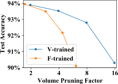
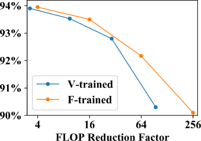
Figure 8: Comparison of objective metrics. Test accuracy versus the volume pruning factor and the FLOP reduction factor for our method with a Volume metric (V-trained) and a FLOP metric (F-trained).

6 Conclusion

We presented a structured budgeted pruning method based on a dropout sparsity learning framework. We proposed a knowledge distillation loss function combined with a budget-constrained sparsity loss whose formulation is that of a barrier function. Since the log-barrier solution is ill-suited for pruning a CNN, we proposed a novel barrier function as well as a novel optimization schedule. We provided concrete insights on how to prune residual networks and used a novel mixed-connectivity block. Results obtained on two ResNets architecture and four datasets reveal that our method outperforms (or is competitive to) 7 other pruning methods.

References

- [1] Stephen Boyd and Lieven Vandenberghe. Convex Optimization. Cambridge University Press, 2004.
- [2] Miguel Carreira-Perpinan and Weiran Wang. Distributed optimization of deeply nested systems. In AI and Stats, pages 10–19, 2014.
- [3] Miguel A Carreira-Perpinán and Yerlan Idelbayev. Learning-compression algorithms for neural net pruning. In Proc. of CVPR, pages 8532–8541, 2018.
- [4] Bin Dai, Chen Zhu, and David P. Wipf. Compressing neural networks using the variational information bottleneck. proc. of ICML, 2018.
- [5] Misha Denil, Babak Shakibi, Laurent Dinh, Nando De Freitas, et al. Predicting parameters in deep learning. In proc of NIPS, pages 2148–2156, 2013.
- [6] Emily L Denton, Wojciech Zaremba, Joan Bruna, Yann LeCun, and Rob Fergus. Exploiting linear structure within convolutional networks for efficient evaluation. In proc of NIPS, pages 1269–1277, 2014.
- [7] Jonathan Frankle and Michael Carbin. The lottery ticket hypothesis: Training pruned neural networks. arXiv preprint arXiv:1803.03635, 2018.
- [8] Yunchao Gong, Liu Liu, Ming Yang, and Lubomir Bourdev. Compressing deep convolutional networks using vector quantization. arXiv preprint arXiv:1412.6115, 2014.
- [9] Ariel Gordon, Elad Eban, Ofir Nachum, Bo Chen, Hao Wu, Tien-Ju Yang, and Edward Choi. Morphnet: Fast & simple resource-constrained structure learning of deep networks. In Proc. of CVPR, 2018.
- [10] Song Han, Jeff Pool, John Tran, and William Dally. Learning both weights and connections for efficient neural network. In proc of NIPS, pages 1135–1143, 2015.
- [11] Babak Hassibi and David G Stork. Second order derivatives for network pruning: Optimal brain surgeon. In proc of NIPS, pages 164–171, 1993.
- [12] Kaiming He, Georgia Gkioxari, Piotr Dollár, and Ross Girshick. Mask r-cnn. In proc. of ICCV, pages 2980–2988, 2017.
- [13] Kaiming He, Xiangyu Zhang, Shaoqing Ren, and Jian Sun. Deep residual learning for image recognition. In Proc. of CVPR, June 2016.
- [14] Geoffrey Hinton, Oriol Vinyals, and Jeff Dean. Distilling the knowledge in a neural network. proc of NIPS DLRL Workshop, 2015.
- [15] Gao Huang, Zhuang Liu, Laurens Van Der Maaten, and Kilian Q Weinberger. Densely connected convolutional networks. In proc. of CVPR, 2017.
- [16] Max Jaderberg, Andrea Vedaldi, and Andrew Zisserman. Speeding up convolutional neural networks with low rank expansions. proc of BMVC, 2014.
- [17] Diederik P Kingma, Tim Salimans, and Max Welling. Variational dropout and the local reparameterization trick. In proc of NIPS, pages 2575–2583, 2015.
- [18] Alex Krizhevsky, Ilya Sutskever, and Geoffrey E Hinton. Imagenet classification with deep convolutional neural networks. In Advances in neural information processing systems, pages 1097–1105, 2012.
- [19] Yann LeCun, John S Denker, and Sara A Solla. Optimal brain damage. In proc of NIPS, pages 598–605, 1990.
- [20] Chenxi Liu, Barret Zoph, Jonathon Shlens, Wei Hua, Li-Jia Li, Li Fei-Fei, Alan Yuille, Jonathan Huang, and Kevin Murphy. Progressive neural architecture search. arXiv preprint arXiv:1712.00559, 2017.
- [21] Z. Liu, J. Li, Z. Shen, G.Huang, S. Yan, and C.Zhang. Learning efficient convolutional networks through network slimming. In proc of ICCV, 2017.
- [22] Christos Louizos, Max Welling, and Diederik P. Kingma. Learning sparse neural networks through regularization. In proc. of ICLR, 2018.
- [23] Z. Luo, F. B-Charron, C. Lemaire, J. Konrad, S. Li, A. Mishra, A. Achkar, J. Eichel, and P-M Jodoin. Mio-tcd: A new benchmark dataset for vehicle classification and localization. IEEE TIP, 27(10):5129–5141, 2018.
- [24] Dmitry Molchanov, Arsenii Ashukha, and Dmitry Vetrov. Variational dropout sparsifies deep neural networks. proc of ICML, 2017.
- [25] Eric Nalisnick and Padhraic Smyth. Unifying the dropout family through structured shrinkage priors. arXiv preprint arXiv:1810.04045, 2018.
- [26] Kirill Neklyudov, Dmitry Molchanov, Arsenii Ashukha, and Dmitry P Vetrov. Structured bayesian pruning via log-normal multiplicative noise. In proc of NIPS, 2017.
- [27] W. Pan, H. Dong, and Y. Guo. Dropneuron: Simplifying the structure of deep neural networks. In arXiv preprint arXiv:1606.07326, 2016.
- [28] Juan-Manuel Pérez-Rúa, Moez Baccouche, and Stephane Pateux. Efficient progressive neural architecture search. arXiv preprint arXiv:1808.00391, 2018.
- [29] Hieu Pham, Melody Y Guan, Barret Zoph, Quoc V Le, and Jeff Dean. Efficient neural architecture search via parameter sharing. arXiv preprint arXiv:1802.03268, 2018.
- [30] Olaf Ronneberger, Philipp Fischer, and Thomas Brox. U-net: Convolutional networks for biomedical image segmentation. In proc of MICCAI, pages 234–241, 2015.
- [31] N. Srivastava, J. Hinton, A. Krizhevsky, I. Sutskever, and R. Salakhutdinov. Dropout: A simple way to prevent neural networks from overfitting. Journal of ML Research, 15:1929–1958, 2014.
- [32] Tom Veniat and Ludovic Denoyer. Learning time-efficient deep architectures with budgeted super networks. In Proc. of CVPR, 2018.
- [33] W.Wen, C Wu, Y.Wang, Y Chen, and H.Li. Learning structured sparsity in deep neural networks. In proc of NIPS, 2016.
- [34] Sergey Zagoruyko and Nikos Komodakis. Wide residual networks. In proc. of BMVC, 2016.
- [35] Barret Zoph and Quoc V Le. Neural architecture search with reinforcement learning. proc of ICLR, 2017.