Asymptotic theory of charged particle transfer reactions at low energies and nuclear astrophysics
R. Yarmukhamedov,1, 4, K. I. Tursunmakhatov,2 and N. Burtebayev3, 4Corresponding author, E-mail:
rakhim@inp.uz
Abstract
A new asymptotic theory is proposed for the peripheral sub- and above-barrier transfer (, ) reaction within the three-body (, and ) model, where = + , = + and is a transferred particle. In the asymptotic theory, the allowance of the contribution of the three-body (, and ) Coulomb dynamics of the transfer mechanism to the peripheral partial amplitudes for the partial wave 1 and of the Coulomb-nuclear distorted effects in the entrance and exit channels is done in a correct manner within the framework of the dispersion theory and the conventional distorted-wave Born approximation (DWBA), respectively. It is shown that the proposed asymptotic theory makes it possible to test the accuracy of taking into account the the three-body Coulomb dynamics of the transfer mechanism in the modified DWBA. The results of the analysis of the differential cross sections of the specific proton and triton transfer reactions at above- and sub-barrier energies are
presented. New estimates and their uncertainties are obtained for values of the asymptotic normalization coefficients for , , and as well as for the direct astrophysical factors at stellar energy of the radiative capture , and reactions.
1Institute of Nuclear Physics, Uzbekistan Academy of Sciences,
Tashkent 100214, Uzbekistan
2 Physical and Mathematical Department of Gulistan State University,
120100 Gulistan city, Uzbekistan
3Institute of Nuclear Physics, 050032 Almaty, Kazakhstan
4 Al Farabi Kazakh National University,
Almaty, 050040, Kazakhstan
PACS: 25.60 Je; 26.65.+t
I. INTRODUCTION
In the last two decades, a number of methods of analysis of experimental data for different nuclear processes were proposed to obtain information on the ‘‘indirect determined’’ (‘‘experimental’’) values of the specific asymptotic normalization coefficients (or respective nuclear vertex constants) with the aim of their application to nuclear astrophysics (see, for example, Refs. [1–5] and the available references therein). One of such methods uses the modified DWBA [6, 7] for nuclear transfer reactions of manifest peripheral character in which the differential cross sections are expressed in the terms of the asymptotic normalization coefficients. One notes that an asymptotic normalization coefficient (ANC), which is proportional to the nuclear vertex constant (NVC) for the virtual decay , determines the amplitude of the tail of the overlap function corresponding to the wave function of nucleus in the binary () channel (denoted by everywhere below) [8]. As the ANC for determines the probability of the configuration in nucleus at distances greater than the radius of nuclear interaction, the ANC arises naturally in expressions for the cross sections of the peripheral nuclear reactions between charged particles at low energies, in particular, of the peripheral exchange , transfer (, ) and astrophysical nuclear reactions.
In the present work, the peripheral charged particle transfer reaction
(1)
is considered in the framework of the three-body (, and ) model, where =() is a projectile, =() and is a transferred particle. The main idea is based on the following two assumptions: i) the peripheral reaction (1) is governed by the singularity of the reaction amplitude at 1, where is the nearest to physical (-1 1) region singularity generated by the pole mechanism
(Fig. 1) [9] and is the scattering angle in the center of mass; ii) the dominant pole played by this nearest singularity is the result of the peripheral nature of the considered reaction at least in the main peak of the angular distribution [10]. Consequently, it is necessary to know the behavior of the reaction amplitude at the nearest singularity [11, 12], which in turn defines the behavior of the true peripheral partial amplitudes at 1
( with ) [13] giving the dominant contribution to the reaction amplitude at least in the main peak of the angular distribution [10, 14], where , , and are a partial wave, a number wave (or a relative momentum), a channel radius, and the radius of the nuclear interaction of the colliding nuclei, respectively.
In practice, the ‘‘post’’-approximation and the ‘‘post’’ form of the modified DWBA [6, 7] are used for the analysis of the specific peripheral proton transfer reactions. They are restricted by the zero- and first-order terms of the perturbation theory over the optical Coulomb polarization operator (or ) in the transition operator, respectively, which are sandwiched by the initial and final state wave functions in the matrix element of the reaction (1). At this, it is assumed that the contribution of the first-order term over (or )
to the matrix element is small [7]. But it was shown in Refs. [2, 12, 15, 16] that, when the residual nuclei are formed in
weakly bound states being astrophysical interest, this assumption is not guaranteed for the peripheral
charged particle transfer reactions and, so,
the extracted ‘‘experimental’’ ANC values may not have
the necessary accuracy for their astrophysical application (see, for example, [16] and Table 1 in [2]). In this case, in
the transition operator an inclusion of all other orders (the second and higher orders) of the power expansion in a series over (or ) is required for the DWBA cross section calculations since they strongly change the power of the peripheral partial amplitudes at 1 [12, 16].
For these reasons, it is of great interest to derive the expressions for the amplitude and the differential cross section (DCS) of the peripheral reaction (1) within the so-called hybrid theory: the DWBA approach and the dispersion peripheral model [10, 11]. The main advantage of the hybrid theory as compared to the modified DWBA is that, first, it allows one to derive the expression for the part of the reaction amplitude having only the contribution from the nearest singularity in which the influence of the three-body Coulomb dynamics of the transfer mechanism on the peripheral partial amplitudes at 1 is taken into account in a correct manner within the dispersion theory. Second, it accounts for the distorted effects in the initial and final states within the DWBA approach, which is more accurate than as it was done in [17] in the dispersion peripheral model [10]. They allow one to treat the important issue: to what extent does a correct taking into account of the three-body Coulomb effects in the initial, intermediate and final states of the peripheral reaction (1), firstly, influence the spectroscopic information deduced from the analysis of the experimental DCSs and, secondly, improve the accuracy of the modified DWBA analysis used for obtaining the ‘‘experimental’’ ANC values of astrophysical interest. Besides, the proposed asymptotic theory can also be applied to strong sub-barrier transfer reactions for which the main contribution to the reaction amplitude comes to several lowest partial waves ( =0, 1,…, where 0 and ) and the contribution of peripheral partial waves ( 1) is strongly suppressed.
It is worth noting that the similar theory was proposed earlier in [14] for the peripheral neutron transfer reaction induced by the heavy ions at above-barrier energies, which was also implemented successfully for the specific reactions. However, for peripheral charged particle transfer reactions this task requires a special consideration. This is connected with the considerable complication occurring in the main mechanisms of the reaction reaction (1) because of correct taking into account of the three-body Coulomb dynamics of the transfer mechanism [11, 12].
Below, we use the system of units = = 1 everywhere, except where they are specially pointed out.
II. THREE-BODY COULOMB DYNAMICS OF THE TRANSFER MECHANISM AND THE GENERALIZED DWBA
We consider the reaction (1) within the framework of the three (, and ) structureless charged particles.
In strict three-body Schrödinger approach, the amplitude for the reaction (1) is given by [18, 19]
(2)
and
(3)
Here and are the optical Coulomb–nuclear distorted wave functions in the entrance and exit channels with the relative momentum and , respectively ( and ); ()(()) is the overlap integral of the bound-state , and (, and ) wave functions [20, 21]; ; ;
= ()-1 is the operator of the three-body (, and ) Green’s function and is the spin projections of the transferred particle , where , () is the nuclear (Coulomb) interaction potential between the centers of mass of the particles and , which does not depend on the coordinates of the constituent nucleus;
and are the optical Coulomb–nuclear potentials in the entrance and exit states, respectively;
in which is the binding energy of the bound () system in respect to the () channel; , is the radius-vector of the center of mass of the particle and = is the reduced mass of the and particles in which is the mass of the particle.
The operator of the three-body Green’s function can be presented as
(4)
where = ()-1 is the operator of the three-body
(, and ) Coulomb Green’s functions; is the kinetic energy operator for the three-body
(, and ) system; and .
Here is the spin
(its projection) of the particle ; , and
( and ) are the total (orbital) angular momentum and its projection of the particle in the nucleus [= ()], respectively;
is the Clebsch-Gordan coefficient, and
is the factor taking into account the nucleons’ identity [8], which
is absorbed in the radial overlap function being not normalized to unity [20]. In the matrix element (5), the integration is taken over all the internal relative coordinates and for the and nuclei.
The asymptotic
behavior of at is given by the relation
(6)
where
is the
Whittaker function, is
the Coulomb parameter for the
bound state, ,
is the nuclear interaction
radius between and particles in the bound () state
and is the ANC for , which is related to the nuclear vertex constant for the virtual decay as [8]
(7)
Eqs. (5)–(6) and the expression for the matrix element for the virtual decay , which is given by Eq. (A1) in Appendix and related to the overlap function , hold for the matrix element of the virtual decay and the overlap function .
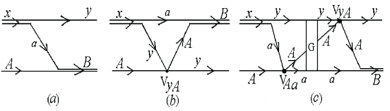
The first () and second () terms, entering the first term of the right-hand side (r.h.s.) of (3), correspond to the mechanisms described by the pole and triangle diagrams in Figs. 1 and 1, respectively, where the Coulomb-nuclear core-core () scattering in the four-ray vertex in the diagram in Fig. 1 is taken in the Born approximation. The term in the r.h.s. of (3) corresponds to more complex mechanisms than the pole and triangle ones. This term is described by a sum of nine diagrams obtained from the basic diagrams presented in Figs. 1 and 1, which take into account all possible subsequent mutual Coulomb-nuclear rescattering of the particles , and in the intermediate state. One of the nine diagrams corresponding to the term is plotted in Fig. 1, where the Coulomb-nuclear ( and ) scatterings in the four-ray vertices, including in all four-ray vertices for the others of eight diagrams, are taken in the Born approximation. This term corresponds to the mechanism of subsequent Coulomb-nuclear rescattering of the and particles, virtually emitted by the projectile , on the target in the intermediate state. In particular, it corresponds to the mechanism of the subsequent rescatterings of the proton () and neutron (), virtually emitted by the deuteron in the field of the target in the nucleon transfer (, ) reaction, where is a nucleon, the transferred particle is either or and = + .
If the reaction (1) is peripheral, then its dominant mechanism, at least in the main peak of the angular distribution, corresponds to the pole diagram in Fig. 1 [10, 14]. The amplitude of this diagram has the singularity at , which is the nearest one to the physical (-1 1) region [9, 10] and is given by the expression
(8)
where and .
However, if we ignore nuclear interactions in the second () and the third () terms of the first term of the r.h.s. of (3) as well as in the one with the help of the corresponding replacement
where and ,
then the amplitude can be presented in the form
(9)
Here
(10)
and
(11)
In Eqs (9)–(11), the contribution of the three-body (, and ) Coulomb dynamics of the transfer mechanism in the intermediate state involves all orders of the perturbation theory over the optical Coulomb polarization potential , whereas the Coulomb-nuclear distortions ( and ) in the entrance and exit channels are taken into account within the framework of the optical model. The amplitude can be considered as generalization of the ‘‘post’’ form of the DWBA amplitude () [22] in which the three-body Coulomb dynamics of the main transfer mechanism are taken into account in a correct manner. One notes that the amplitude passes to the amplitude of the so-called ‘‘post’’-approximation of the DWBA if all the terms of contained in the transition operators of Eqs. (10) and (11) are ignored.
III. DISPERSION APPROACH AND DWBA
The amplitudes given by Eqs. (10) and (11) have the nearest singularity (the type of branch point), which defines the behavior both of the amplitude at = [12] and of the true peripheral partial amplitudes at 1 [13]. Besides, owing to the presence of nuclear distortions in the entrance and exit states, these amplitudes have also the singularities located farther from the physical region than . Nevertheless, the behavior of the near , denoted by below, can be presented as:
(12)
(13)
Here is the behavior of the amplitude near [12], which corresponds to the mechanism described by the diagram in Fig. 1 and is determined from Eq. (10) if the term in the transition operator is ignored. In (13), is the Coulomb renormalized factor (CRF) for the pole-approximation of the DWBA amplitude and is the CRF for the amplitude. The explicit forms of the CRFs and are given in Eqs. (14) and (26) of [12]. As for, the behavior of the singular part of the amplitude at = , as is pointed out in [12], it has the identical behaviour as that for
the
amplitude. But, the task of directly finding the CRF explicit form of the amplitude is fairly difficult because of the presence of the three-body Coulomb operator in the transition operator and, so, it requires a special consideration, especially, in the so-called ‘‘dramatic’’ case [12]. In this case, the partial wave amplitudes with 1 generating the behavior of the amplitude at = provide the essential contribution to the amplitude [12]. For example, as it is noted in [16], the peripheral and reactions considered in [23, 24, 25] within the ‘‘post’’ form of the MDWBA are related in the ‘‘dramatic’’ case. Perhaps, that is one of the possible reasons why the ANC value for recommended in [25] is underestimated, which lead in turn to the underestimated astrophysical factor for the direct radiative capture reaction at solar energies [26]. The analogous case occurs for the peripheral reaction, which was analyzied in [27] within the same MDWBA. This fact dictates the further updating of the asymptotic theory proposed in the present work, where the ‘‘dramatic’’ case will also be included. At present such work is in progress.
Nevertheless, in the ‘‘non-dramatic’’ case, the accuracy of the amplitude can be defined by the extent of proximity of the CRF and the true CRF corresponding to the amplitude [12] (see Table 2 in [12]). The explicit form of has been obtained in [11] from the exact (in the framework of the three-body (, and ) charged particle model) amplitude of the sub-barrier reaction (1) and is given in Refs. [11, 12]. Then the behavior of the exact amplitude, denoted by below, near the singularity at = takes the form as
(14)
where
(15)
One can see that the , and amplitudes
have the same behaviour near the singular point at = . But, they differ from each other only by the power. These amplitudes define the corresponding peripheral partial amplitudes for 1, which differ also from each other by their power [13].
Therefore, below we will first show how to obtain the singular part of the by separating the contribution from the nearest singularity to it. Then, from the expression derived for this amplitude we obtain the generalized DWBA amplitude in which the contribution of the three-body (, and ) Coulomb dynamics of the main transfer mechanism to the peripheral partial amplitudes for 1 are taken into account in a correct manner.
IV. DISTORTED-WAVE POLE APPROXIMATION
The pole-approximation of the DWBA amplitude can be obtained from Eq.
(10). It has the form as
(16)
Here , and
(17)
where = , = , = and = .
To obtain the explicit singular behavior of at , the integral (16) should be rewritten in the momentum representation making use of Eq. (A1) from Appendix. It takes the form
(18)
(19)
Here is the off-shell of the Born (pole) amplitude; (), () and are the Fourier components of the distorted wave function in the entrance (exit) channel, the overlap function for the bound ( + ) (( + )) state and the Coulomb-nuclear potential, respectively; and , where and . The explicit form of is similar to that for the virtual decay given by Eq. (A1) in Appendix.
Using Eq. (A1) from Appendix and the corresponding expression for , the amplitude can be presented in the form
(20)
Here
and
(21)
where ; ; () is the set of and () and
(22)
are the reduced vertex functions for the virtual decays and , respectively.
In the presence of the long-range Coulomb interactions between particles and ( and ), the reduced vertex function for the virtual decay () can be described by the sum of the nonrelativistic diagrams plotted in Fig. 2. The diagram in Fig. 2 corresponds to the Coulomb part of the corresponding vertex function, which has a branch point singularity at the point =0 ( = 0) and generates the singularity of the amplitude at = . The sum in Fig. 2 involves more complicated diagrams and this part of the vertex function corresponds to the Coulomb-nuclear vertex function, which is regular at the point (). Then, the vertex functions and can be presented in the forms [28]
(23)
Here and
( and ) are the Coulomb part and the regular function at the point (), respectively.
All terms of the sum in Fig. 2 have dynamic singularities, which are generated by internuclear interactions being responsible for taking into account of the so-called dynamic recoil effects [19, 22]. These singularities are located at the points and [29, 30], where , , and . They generate the singularities and of the amplitude, which are determined by
and
As a rule, they are located farther from the physical (-1 1) region than ( and ) [28, 29]. For illustration of the fact, the position of these singularities (, and ), , and calculated for the specific peripheral reactions considered in the present work are presented in Table 1. As can be seen from Table 1, the singularities and are located farther from the physical (-1 1) region than the singularity .
For the surface reaction (1), the contribution of the interior nuclear range to the amplitude, which is generated by the singularities of the and functions, can be ignored at least in the main peak of the angular distribution [10, 14]. Therefore, the vertex functions for the virtual decays and given by Eq. (22) can be replaced by their Coulomb parts in the vicinity of nearest singularities (the branch points) located at
and , respectively. They behave as [28]
(24)
for , where ) is the NVC for the virtual decay ; = ; = and = for the virtual decay , whereas = and = for the virtual decay .
As is seen from Eqs. (20), (21) and (24), the off-shell Born amplitude at = and = has the nearest dynamic singularity at = .
Besides, has also kinematic singularities generated by the factors
and in
(20) [10]. Nevertheless, we take into account the contribution generated by the kinematic singularities to the amplitude. Then given by (20) in the approximation (24) takes the form
(25)
where
(26)
(27)
We now rewrite the integral (18) taking into account
Eqs. (25) – (27) in the coordinate representation. First, we consider this presentation for the Fourier components of the and functions:
(28)
and
(29)
Substituting Eq. (26) in Eq. (28) and Eq. (27) in Eq. (29), the integration over the angular variables can immediately be performed making use of the expansion
where is a spherical Bessel function [31]. The remaining integrals in and can be done with the use of formula 6.565(4) and Eq. (91) from Refs. [32] and [8], respectively. As a result, one obtains
(30)
for and
(31)
for . Here is a modified Hankel function [31] and is the radius of nucleus, where is a mass number of the nucleus. Using formula 9.235 (2) from [32] and the relation (7), the leading asymptotic terms of Eqs. (30) and (31) can be reduced to the forms
(32)
for and
(33)
for . In (32), is the Coulomb interaction potential between the centers of mass of particles and , and
(34)
which coincides with the leading term of the asymptotic behavior of the radial component of the overlap function for .
Following by the way of [30], it can be shown that the leading terms of the asymptotic expressions for
the radial components of the Coulomb-nuclear parts of and (Fig.2), which are generated by the singularities of and , respectively, behave as
(35)
Here
(36)
(37)
Explicit expressions for and can be obtained from Eqs. (A.4) and (A.5) of [30], which are expressed in the terms of the product of the ANCs for the tri-rays vertices of the diagrams in Fig. 2. As is seen from the expressions (35), (36) and (37), if and
, which occur for the peripheral reactions presented in Table 1, then the asymptotic terms generated by the singularities and of the amplitude decrease more rapidly with increasing and , respectively, than those of (32) and (33) generated by the singularity .
Therefore, the use of the pole approximation is reasonable in calculations of the leading terms of the peripheral partial wave amplitudes at 1. They correctly give the dominant contribution to the at least in the main peak of the angular distribution and are correctly determined by only the nearest singularity [13].
Thus, usage of the pole approximation in the amplitude (16) is equivalent to the replacements of and by and in the integrand of Eq. (16), respectively. In this case, in the coordinate representation,
the amplitude can be reduced to the form as
(38)
where
(39)
One notes that the expression (30) for is valid for and becomes identically zero for = 0. In this case, the Fourier component of the function in (28) is given only by the kinematic function for 0 and, so, the Fourier integral becomes singular [14]. Therefore, according to [14], for = 0 this case should be considered specially by putting = 0 in the integrand of Eq. (28) a priori. Then, for = 0 one obtains
(40)
where is given by Eq. (17) and = . This expression corresponds to the well-known zero-range approximation [14] and can be used jointly with Eq. (31) in the amplitude, for example, for the peripheral (, ) reaction.
We now expand the amplitude in partial waves. To this end, in (39) we use the partial-waves expansions (A2) given in Appendix and the expansion
(41)
Here
(42)
where = [()2 + ()2 - 2]1/2, = [()2 + ()2 - 2]1/2 and = . The integration over the angular variables and in Eq. (39) can easily be done by using Eqs. (A3) and (A4) from Appendix. After some simple, but cumbersome algebra, one finds that the pole amplitude in the system has the form
(43)
where the explicit form of is given by Eqs. (A7) -(A10) in Appendix.
It should be noted that just neglecting the dynamic recoil effect mentioned above, which is caused by using the pole approximation in the matrix elements for the virtual decays and
, results in the fact that the radial integral (A8) of the amplitude does not contain the and potentials in contrast to that of the conventional DWBA with recoil effects [19, 22]. That is the reason why the amplitude is parametrized directly in the terms of the ANCs but not in those of the spectroscopic factors as it occurs for the conventional DWBA [19, 22].
V. THREE-PARTICLE COULOMB DYNAMICS OF THE TRANSFER MECHANISM AND THE GENERALIZED DWBA
We now consider how to accurately take into account the contribution of the three-body Coulomb dynamics of the transfer mechanism to the and amplitudes by using Eqs. (14), (15) and (43) as well as Eqs. (A7) and (A8) from Appendix. To this end, we should compare partial wave amplitudes
and for 1 determined from the corresponding expressions for the and amplitudes [11, 12].
According to [13], from Eq. (14) and (15), the peripheral partial amplitudes at 1 and 1 can be presented in the form as
(44)
Here is the
peripheral partial amplitude corresponding to the pole approximation of the DWBA amplitude and , where
,
and is -Euler’s function. One notes that the CRF is complex number and depends on the energy , the binding energies and as well as the Coulomb parameters (, , and ), where and are the Coulomb parameters for the entrance and exit channels, respectively. The expression for given by (44) can be considered as the peripheral partial amplitude of the generalized DWBA in which the contribution of the three-body Coulomb dynamics of the main transfer mechanism is correctly taken into account.
As is seen from here, for 1 and 1 the asymptotics of the pole approximation () of the DWBA and the exact three-body partial amplitudes () have the same dependence on and . Nevertheless, they differ only in their powers.
Therefore, if the main contribution to the amplitude comes from the peripheral partial waves with 1 and 1, then the expression (44) makes it possible to obtain the amplitude of the generated DWBA. For this aim, the expression , which enters the pole approximation of the DWBA amplitude given by Eq. (43) as well as Eqs. (A7) and (A8),
has to be renormalized by the replacement
(45)
Here
(46)
where (or ).
From Eqs. (43), (45) and (46), we can now derive the expression for the differential cross section for the generalized three-body DWBA. It has the form as
(47)
where the expression for is obtained from Eq. (A7) of Appendix by the substitution of the by given by (45). Herein, the ANCs ’s , and are in fm-1/2, fm-1 and mb/sr, respectively. One notes that Eqs. (47) and (A8) given in Appendix contain the cutoff parameters and , which are determined by only the free parameter . Similar to how it was done in Ref. [14], the value can be determined by best fitting the calculated angular distributions to the experimental ones corresponding to the minimum of at least in the angular region of the main peak.
One notes that the expression (47) can be considered as a generalization of the dispersion theory proposed in Ref. [14] for the peripheral neutron transfer reactions at above-barrier energies. Nevertheless, the expression (47) can also be applied for peripheral strong sub-barrier charged particle transfer reactions for which the dominant contribution comes to rather low partial waves with (or )= 0,1, 2,… In this case, the influence of the three-body Coulomb dynamics of the transfer mechanism on the DCS is also taken into account via the interference term between the low and peripheral partial amplitudes entering Eq. (47) via Eq. (46).
VI. RESULTS OF APPLICATIONS TO THE SPECIFIC SUB- AND ABOVE-BARRIER REACTIONS
A. Asymptotic normalization coefficients
In order to verify predictions of the asymptotic theory proposed in the present work and the influence of the three-body Coulomb dynamics of the transfer mechanism on the specific ANC values, we have calculated the differential cross sections of the proton and triton transfer reactions: at the bombarding energy = 100 MeV
[7]; at = 87 MeV [22]; at = 29.75 MeV [34] and
at sub-barrier energies = 250; 350 and 450 keV [35, 36] (denoted by EXP-1978 below) as well as = 327; 387 and 486 keV [37] (denoted by EXP-2015 below). One notes that all these reactions are related to the ‘‘non-dramatic’’ case.
Calculations were performed using Eq. (47) and the optical potentials in the initial and final states, which were taken from Refs. [7, 22, 34, 36]. For these reactions the orbital ( and ) and total ( and ) angular momentums of the transfer particle (proton or triton) are taken equal to == 1, = 2 and == 0, whereas == 3/2, = 5/2 and = = 1/2.
The results of the calculations of the CRFs for the considered reactions, which take into account the influence of the three-body Coulomb dynamics on the peripheral partial amplitudes, are listed in Table 2. There, the calculated values of correspond to the CRF for the ‘‘post’’ form of DWBA [22], and is determined by the ratio of the CRF to that
(=
),
where = and the explicit form of the CRF is determined from the expressions (14), (24)–(26) of Ref. [12]. As is seen from Table 2, the differences between the calculated CRFs and are fairly larger than that between the calculated CRFs and . This fact indicates that the terms and of the transition operator, which enter the right-hand side of the amplitudes Eqs. (10) and (11), respectively, give a fairly large contribution to the peripheral partial amplitudes at 1 and 1 of the
amplitude (9). For an estimate of the influence of the CRFs on the calculated peripheral partial amplitudes,
we have analyzed the contribution of the different partial wave amplitudes to the amplitude both for the sub-barrier reactions and for the above-barrier one mentioned above. Fig. 3 shows the dependence of the modulus of the partial amplitudes, which are renormalized on the product of the ANCs for the bound states of the nuclei in the entrance and exit channels. As is seen from Figs. 3 and 3, the contribution to the amplitude of the and reactions from lower partial amplitudes with 14 and 15, respectively, is strongly suppressed due to the strong absorption in the entrance and exit channels. Nevertheless, for the transferred angular momentum = 0 the contributions of the three-body Coulomb effects to the modulus of the partial amplitudes () change from 55% to 7% for the reaction at 16 and from 23% to 5% for the one at 21 (see the inset in Fig.3). It should be noted that the orbital angular momenta for these reactions are 16 and 21 for the channel radius 5.3 and 5.6 fm, respectively. The analogous contribution is found to be about 20–30% for the (g.s.) reaction for which 8 for the channel radius 5 fm (see the inset in Fig.3). For the (0.495 MeV) reaction the influence of the three-body Coulomb effects on the peripheral partial amplitudes is extremely larger as compared with that for the (g.s.) reaction. For example, the ratio of the calculated with taking into account of the CRF of (see Eqs. (45) and (46)) to that calculated without taking into account of the CRF (= 1) in the peripheral partial amplitudes changes about from 1.3x10⁻⁷ to 2.2x10⁻⁷ for 13.
This is the result of the strong difference between the ratio calculated for the ground and fist exited states of the residual nucleus (see Table 2). In Fig. 3, as an illustration, the same dependence is displayed for the sub-barrier reaction at the energy = 0.250 MeV for which 1 corresponding to the channel radius 5 fm. As is seen from Fig. 3, the contribution of the peripheral partial wave to the reaction amplitude is strong suppressed, whereas the main contribution to the amplitude comes to the low partial waves in the vicinity of 1. The analogous dependence occurs for other considered energies .
As is seen from here, the influence of the three-body Coulomb effects in the initial, intermediate and final states of the considered above-barrier reactions on the peripheral partial amplitudes of the reaction amplitude can not be ignored. One notes that this influence is ignored in the calculations of
the‘‘post’’-approximation and the ‘‘post’’ form of the DWBA performed in [6] and [7, 22], respectively. In this connection, it should be noted that this assertion is related also to the calculations of the dispersion peripheral model performed in [28] for the peripheral proton transfer reactions with taking into account only the mechanism described by the pole diagram in Fig. 1. Perhaps that is one of the possible reasons why the NVC (ANC) values for the specific virtual decay , derived in [28] with and without taking into account the Coulomb effects in the vertices of the pole diagram in Fig. 1, differ strongly from each other (see Table in [28]).
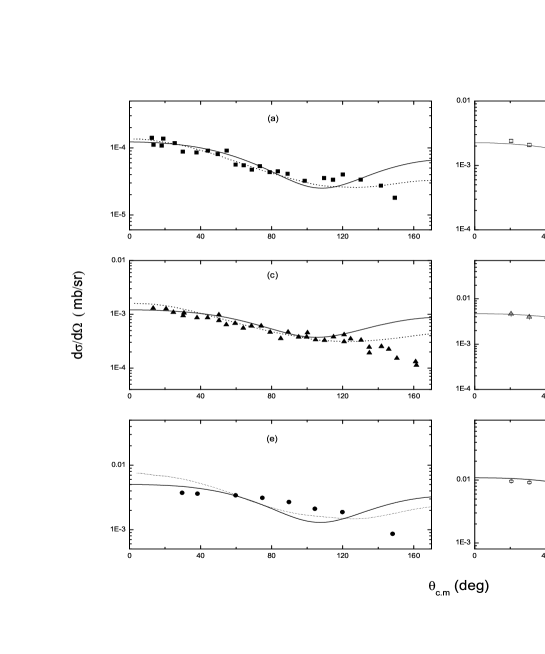
The results of the calculations and of the comparison between the differential cross sections obtained in the present work (the solid curves), the DWBA obtained in Refs. [7, 22, 36, 37] by other authors (the dash curves) and experimental data are shown in Figs. 4 – 6 and summarised in Table 3. In the calculations we made use of the two different optical potentials (the sets 1 and 2) taken from Refs. [7, 34] and the optical potentials taken from [22, 36]. The results of the present work correspond to the standard value for the parameter, which is taken equal to 1.25 fm and leads also to the minimum of in the vicinity of the main peak of the angular distribution. It is seen that the angular distributions given by the asymptotic theory and the conventional DWBA practically coincide and reproduce equally well the experimental ones. The ANCs (NVCs) values obtained in the present work, which are presented in Table 3, are found by normalizing the calculated cross sections to the corresponding experimental ones at the forward angles by using the ANCs =4.200.32 fm-1 [26] (= 1.320.10 fm) for and = 54.24.5 fm-1[39] (= 13.41.1 fm ) for . There, the theoretical and experimental uncertainties are the result of variation (up to 2.5%) of the cutoff and (or ) parameters relative to the standard and ( = = 1.25 fm) values and the experimental errors in .
But, the experimental uncertainties pointed out in the ANC (NVC) values for and correspond to the mean squared errors, which includes both the experimental errors in and the above-mentioned uncertainty of the ANC (NVC) for and , respectively.
As is seen from Table 3, the squared ANC value for obtained in the present work differs noticeably from that of [7] derived from the analysis of the same reaction performed within the framework of the ‘‘post’’ form of the modified DWBA. Besides, as can be seen from Table 3, the difference between the squared ANC values obtained in the present work for the set 1 and the set 2 of the optical potentials (the second and fifth lines) does not exceed overall the experimental errors (= 7% [7]) for the differential cross section, whereas such the difference for the squared ANC values derived in [7] (the third and sixth lines) exceeds noticeably and is of about 9%.
The ANC for recommended in the present work is presented in the seventh and eighth lines of Table 3, which has overall the uncertainty of about 4%. An analogous situation occurs when we compare the results for the ANC for (g.s) and (0.429 MeV) between the present work (the 19th and 30th lines), Ref. [34] ( the 20th and 31th lines) and Ref. [6] ( the 21th and 32th lines).
Besides, it is seen that the discrepancy between the ANC values of the present work and Ref. [6] is larger than that of [34]. One notes once more that the ‘‘post’’-approximation and the ‘‘post’’ form of the modified DWBA were used in [6] and [34], respectively. Nevertheless, the ANCs derived in the present work are in a good agreement within the uncertainties with the results recommended in [38](see the 22th and 33th lines of Table 3).
It is seen that the asymptotic theory proposed in the present work provides better accuracy for the ANC values for and than that obtained in Refs. [7, 34, 38].
The ANC values for
and obtained in the present work are presented the eleventh and 34th – 43th lines of Table 3, respectively. As is seen from there, the ANC values obtained separately from the analysis of the experimental data taken from Refs.[35] (EXP-1978) and [37](EXP-2015) differ from each other on the average by a factor of about 2.2. This is the result of the discrepancy between the absolute values of the experimental DCSs of the EXP-1978 and the EXP-2015 measured independently each other. Because of a presence of such the discrepancy, we recommended decisive measurement of the experimental DCSs of the reaction in the same energy region. Nevertheless, one notes that the ANCs obtained separately from the independent experimental data of the EXP-1978 and EXP-2015
at the different projectile energies are stable, although the absolute values of the corresponding experimental DCSs depend strongly on the projectile energy (see Fig. 6). To best of our knowledge, the ANC values for and presented in Table 3 are obtained for the first time.
B. Astrophysical factors at stellar energies
Here the weighted means of the ANCs obtained for (g.s.) and (0.429 MeV), (g.s.) and (g.s.) are used to calculate the astrophysical factors for the radiative capture (g.s.), (0.429 MeV), (g.s.) and (g.s. ) reactions at stellar energies. The calculations are performed using the modified two-body potential method [40] for the direct radiative capture reaction and the modified -matrix method only for the direct component of astrophysical factors for the radiative capture (g.s.) and (g.s.) (see Ref. [41] for example).
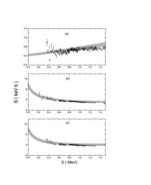
Fig. 7 shows the results of comparison between the astrophysical factors calculated for the radiative capture reaction and the experimental data [42]. There, the solid curves in () and () present the results obtained in the present work for the ground and first excited (= 0.429 MeV) states of the residual nucleus, respectively, whereas the solid curve in () corresponds to their sum
(g.s. + 0.429 MeV). There, the bands are the corresponding uncertainties arising because of the uncertainties of the ANCs. The dashed lines in Fig. 7 are taken from Ref. [38]. As is seen from figure, the ANC values obtained in the present work for (g.s.) and (0.429 MeV), firstly, reproduce well the experimental data and, secondly, allow extrapolation of the astrophysical factors (()) at stellar energies. In a particular, ()= 0.440.04 and 0.450.05 keVb, ()= 9.891.01 and 9.200.94 keVb and ()= 10.341.06 and 9.750.98 keVb are obtained for = 0 and 25 keV, respectively. One notes that our result for = 0 agrees with that of (0)=9.450.4 keVb recommended in [38] as well as with the results of 10.2 and 11.0 keVb obtained in [43] within the framework of the microscopic model for the effective V2 and MN potentials of the NN potential, respectively.
The results obtained in the present work for the direct component of direct astrophysical factors (()) for the (g.s.) are equal to ()=0.1730.0076 and 0.1710.0075 keVb at =0 and 25 keV, respectively. Whereas, for the (g.s.) reaction they are equal to ()=0.1900.008 and 0.1870.008 keVb at =0 and 25 keV, respectively. We note that our result for (0) for the (g.s.) is in a good agreement with that of [44] (within about 2) and larger (by about 4.7) than that recommended in [45]. This is a result of the discrepancy between the ANC values recommended in the present work and Ref. [7] (see Table 3).
VII. CONCLUSION
Within the strong three-body Schrödinger formalism combined with the dispersion theory, a new asymptotic theory is proposed for the peripheral sub- and above-barrier charged-particle transfer (, ) reaction, where =( + ), =( + ) and is the transferred particle. There, the contribution of the three-body (, and ) Coulomb dynamics of the transfer mechanism to the reaction amplitude is taken into account in a correct manner, similar to how it is done in the dispersion theory. Whereas, an influence of the distorted effects in the entrance and exit channels are kept in mind as it is done in the conventional DWBA. The proposed asymptotic theory can be considered as a generalization of the ’’post’’-approximation and the ‘‘post’’ form of the conventional DWBA in which the contributions of the three-body Coulomb effects in the initial, intermediate and final states to the main pole mechanism is taken correctly into account in all orders of the parameter of the perturbation theory over the Coulomb polarization potential .
The explicit form for the differential cross section (DCS) of the reaction under consideration is obtained, which is directly parametrized in the terms of the product of the squared ANCs for + and + being adequate to the physics of the surface reaction. In the DCS, the contributions both of the rather low partial waves and of the peripheral partial ones are taken into account in a correct manner, which makes it possible to consider both the sub-barrier transfer reaction and the above-barrier one simultaneously.
The asymptotic theory proposed in the present work has been applied to the analysis of the experimental differential cross sections of the specific above- and sub-barrier peripheral reactions corresponding to the proton and triton transfer mechanisms, respectively. It is demonstrated that it gives an adequate description of both angular distributions in the corresponding main peaks of the angular distributions and the absolute values of the specific ANCs (NVCs). The ANCs were also applied to calculations of the specific nuclear-astrophysical radiative proton capture reactions and new values of the astrophysical factors extrapolated at stellar energies were obtained.
ACKNOWLEDGEMENT
This work has been support in part by the Ministry of Innovations and Technologies of the Republic of Uzbekistan (grant No. HE F2-14) and by the Ministry of Education and Science of the Republic of Kazakhstan (grant No. AP05132062).
APPENDIX: Formulae and expressions
Here we present the necessary formulae and expressions.
The matrix element of the virtual decay is related to the overlap function as [8]
where is the vertex formfactor for the virtual decay , is the relative momentum of the and particles and , i.e., the NVC coincides with the vertex formfactor
when all the , and particles are on-shell ().
The same relations similar to Eq. (A1) hold for the matrix element of the virtual decay and the overlap function .
The partial-waves expansions for the distorted wave functions of relative motion of the nuclei in the initial and exit states of the reaction under consideration have the form as [19]
where is the partial wave functions in the initial state or the final one.
The expansions of the and functions on the bipolar harmonics of the rank and the one have the forms as
The explicit form of entering Eq. (43) is given by
where and are Rakah and Fano coefficients [33], respectively; () is the cutoff radius in the entrance (exit) channel; is the binomial coefficient and = .
References
[1]
L. D. Blokhintsev, R. Yarmukhamedov, S. V. Artemov, I. Boztosun, S. B. Igamov, Q. I. Tursunmakhtov, and M. K. Ubaydullaeva, Uzb. J. Phys. 12, 217 (2010).
[2]
R. Yarmukhamedov, and Q. I. Tursunmahatov, The Universe Evolution: Astrophysical and nuclear aspects. Edit. I. Strakovsky and L. D. Blokhintsev.
(New York, NOVA publishers, 2013), pp.219–270.
[3]
R. E. Tribble, C. A. Bertulani, M La Cognata, A. M. Mukhamedzhanov, and C. Spitaleri, Rep. Prog. Phys. 77, 901 (2014).
[4]
L. D. Blokhintsev, V. I. Kukulin, A. A. Sakharuk, D. A. Savin, and E. V. Kuznetsova, Phys. Rev. C 48, (1993).
S. B. Igamov, and R. Yarmukhamedov, Nucl. Phys. A 781, 247
(2007).
[5]
R. Yarmukhamedov and D. Baye, Phys. Rev. C 84, 024603 (2011).
[6]
S. V. Artemov, I. R. Gulamov, E. A. Zaparov, I. Yu. Zotov, and G. K. Nie,
Yad. Fiz. 59, 454 (1996)[Phys. At. Nucl. 59, 428 (1996)].
[7]
A. M. Mukhamedzhanov, H. L. Clark, C. A. Gagliardi, Y.-W. Lui, L. Thache,
R. E. Thibble, H. M. Xu, X. G. Zhoú, V. Burjan, J. Cejpek, V. Kroha, and F. Carstoiu, Phys. Rev. C 56, 1302 (1997).
[16]
S.B. Igamov, M.C. Nadyrbekov and R. Yarmukhamedov, Phys.At.Nucl. 70, 1694 (2007).
[17]
E.I. Dolinskii, A.M. Mukhamedzhanov, R. Yarmukhamedov, Direct Nuclear Reactions on Light Nuclei With Detected
Neutrons (FAN, Tashkent, 1978), pp. 7–49 (in Russian).
[18]
K. R. Greider, L. R. Dodd, Phys.Rev. 146, 671 (1966).
[19]
N. Austern, R. M. Drisko, E. C. Halbert, G. R. Satchler, Phys.Rev. 133, B3 (1964).
[20]
T. Berggren, Nucl. Phys. 72, 337 (1965).
[21]
W. T. Pinkston, and G. R. Satchler, Nucl. Phys. 72, 642 (1965).
[22]
R. M. DeVries, Phys. Rev. C 8, 951 (1973).
[23]
A. Azhari, V. Burjan, F. Carstoiu, H. Dejbakhsh, C.A. Gagliardi, V. Kroha, A.M. Mukhamedzhanov, L. Trache and R. E. Tribble, Phys.Rev. Lett. 82, 3960 (1999).
[24]
A. Azhari, V. Burjan, F. Carstoiu, C. A. Gagliardi, V. Kroha, A. M. Mukhamedzhanov, X. Tang, L. Trache and R. E. Tribble, Phys.Rev. 60, 055803 (1999).
[25]
G. Tabacaru, A. Azhari, J. Brinkley, V. Burjan, F. Carstoiu, Changbo Fu, C. A. Gagliardi, V. Kroha, A.M. Mukhamedzhanov, X. Tang, L. Trache, R. E. Trible and S. Zhou, Phys.Rev. C 73, 025908 (2006).
[26]
R. Yarmukhamedov, L. D. Blokhintsev, Phys. At. Nucl. 81, 616 (2018).
[27]
X. Tang, A. Azhari, Changbo Fu, C. A. Gagliardi, A. M. Mukhamedzhanov, F. Pirlepesov, L. Trache, R. E. Tribble, V. Burjan, V. Kroha, F. Carstoiu, and B.F. Irgaziev, Phys.Rev.C 69, 55807 (2004).
[28]
P. O. Dzhamalov, and E. I. Dolinskii, Yad. Fiz. 14, 753 (1971) [Sov. J. Nucl. Phys. 14, 453 (1971)].
[30]
L. D. Blokhintsev, A. M. Mukhamedzhanov, R. Yarmukhamedov, Eur. Phys. J. A 49, 108 (2013).
[31]
M. Abramowitz, I.A. Stegun, Handbook of Mathematical Functions
(Dover, New York, 1970).
[32]
I.S. Gradshteyn, I.M. Ryzhik, Tables of Integrals, Series, and
Products(Academic Press, New-York, 1980).
[33]
D.A. Varshalovich, A.N. Moskalev, and V.K. Hersonskii,
Kvantovaya teoriya uglovogo momenta (Quantum theory of the angular
momentum)(Nauka, Leningrad, 1973)(in Russian).
[34] C.A. Gagliardi,
R.E. Tribble, A. Azhari, H.L. Clark, Y.-W. Lui, A.M Mukhamedzhanov, A.
Sattorov, L. Trache, V. Burjan, J. Cejpek, V. Kroha, S. Piskor, and J.
Vincour, Phys. Rev. C 59, 1149 (1999).
[35]
H. Lorenz-Wirzha, Ph.D. thesis, Universität, Müster, 1978.
[36]
H. Herndl, H. Abele, G. Staudt, B. Bach, K. Grün, H. Scsribany, H. Oberhummer, G. Raimann, Phys. Rev. C 44, R952 (1991).
[37]
I. Lombardo, D. Dell’Aquila, A.Di Leva, I. Indelicato, M. La Cognata, M. La Commara, A. Ordine, V. Rigato, M. Romoli, F. Rosalo, G. Spadaccini, C. Spitareli, A. Tumino and M. Viliance, Phys. Lett. B 778, 178 (2015).
[39]
G. R. Plattner, R. D. Viollier, D. Trautmann, K. Alder, Nucl. Phys. A 206, 513 (1973).
[40]
S.B. Igamov, and R. Yarmukhamedov, Nucl.Phys.A 781, 247
(2007);A 832, 346 (2010).
[41]
S. V. Artemov, S. B. Igamov, Q. I. Tursunmakhatov, and R. Yarmukhamedov, Phus. Atom. Nucl. 75, 291 (2012).
[42]
R. Morlock, R. Kuns, A. Maye, et al. Phys. Rev. Lett. 79, 3837 (1997).
[43]
D. Baye, P. Descouvemont, and M. Hesse, Phys. Rev. C 58 (1998) 545.
[44]
E. A. Wulf, M. A. Godwin, J. F. Guillemette, C. M. Laymon, R.M. Prier, B.J. Rice, V. Spraker, D.R. Tilley, H.R. Weller, Phys. Rev. C 58, (1998) 517.
[45]
A. Sattarov, A. M. Mukhamedzhanov, A. Azhari, C. A. Gagliardi, L. Trache, and R. E. Trible, Phys. Rev. C 60, 035801 (1999).
Figure 1: Diagrams describing transfer of the particle and taking into account possible subsequent Coulomb-nuclear rescattering of particles (, and ) in the intermediate state.Figure 2: Diagrams describing the matrix element for the virtual decay ().Figure 3: The dependence of the modulus of the partial wave amplitudes () for the (), (), (g.s.) () and () reactions at projectile energies of = 100 MeV, = 87 MeV, = 29.75 MeV and =250 keV. Here and are the relative orbital momenta in the entrance and exits channels of the considered reaction, respectively, and is the transferred angular momentum. In () and (), the solid line is for = 0 and , the dashed line is for = 1 and and the dotted line is for = 2 and . In (), the solid line is for = 2 (). In (), the solid line is for = 0 (). The inserts are the ratio of the calculated with taking into account of the CRF of (see Eqs. (45) and (46)) in the peripheral partial waves to that calculated with = 1 in the peripheral partial amplitudes. Figure 4: The differential cross sections for the () and () reactions at = 100 MeV and = 87 MeV, respectively. The solid curves are the results of the present work, whereas the dashed
lines are the results of Refs. [22] and [7] derived in the conventional and modified DWBA, respectively.
The experimental data are taken from Refs. [7, 22].Figure 5: The differential cross sections for the reaction corresponding to the ground () and first excited (0.429 MeV ()) states of at = 29.75 MeV. The solid and dashed curves are the results of the present work and those of Ref. [34] derived in the ‘‘post’’ form of the modified DWBA.
The experimental data are taken from Refs. [34]. Figure 6: The differential cross sections for the reaction at = 450 (), 350 () and 250 keV () (the left side) as well as = 327 (), 387 () and 486 keV () (the right side). The solid curves are the results of the present work, whereas the dashed lines are the results of Ref. [36] derived in the zero-range of the ‘‘post’’-approximation of DWBA. The experimental data are taken from Refs. [35] (the EXP-1978:(), () and (), see [36] too) and [37] (the EXP-2015:(), () and ()).Figure 7: The
astrophysical factors for the direct radiative capture reaction. The curves of () and () correspond to the ground and first excited (0.429 MeV) states of the residual nucleus, respectively, whereas that of () corresponds to their sum
(g.s. + 0.429 MeV).
The solid and the band are the results of
the present work, whereas the dashed line is the result of Ref. [38]. The experimental data are from [42].
Table 1: The specific reactions and the corresponding to them vertices described by the triangle diagram Fig. 2, the positions of singularities and () in () as well as and () in the -plane of the reaction amplitude, where is related either to the vertex B A+ ( = ) or to the vertex x y+ (= ) .
The vertex
Reaction
(),
(, )
MeV
()
(, fm-1)
()
()
()
fm-1
()
(, )
100
1.020(0.534)
0.940
1.064
2.024
1.479
0.802
4.169
(, )
87
1.037(0.840)
2.131
1.264
2.059
1.384
1.618
16.020
(, )(g.s.)
29.7
1.065(0.165)
2.696
3.253
2.645
3.508
0.905
49.551
()
1.065( 0.420)
()
()
()
(0.652)
(1.562)
(, )
0.250
13.648(1.194)
1.522
19.720
0.350
11.544(1.194)
1.522
16.647
0.450
10.190(1.194)
1.522
14.665
Table 2: Reaction (, ), incident energy , values of CRFs and as well as in the pole-approximation and the ’’post’’ form of DWBA as well as the three-body model, respectively, and quantities = , = and .
Table 3: Reaction, energy , set of the optical potentials (set), virtual decay , orbital and total angular momentums (, ), square modulus of the nuclear vertex constant ( ) for the virtual decay and the corresponding ANC () . Figures in brackets are experimental and theoretical uncertainty, respectively, whereas those in square brackets are weighed mean derived from the ANCs (NVCs) values for the sets 1 and 2.