Ideal Quantum Nondemolition Readout of a Flux Qubit Without Purcell Limitations

Abstract

Dispersive coupling based on the Rabi model with large detuning is widely used for quantum nondemolition (QND) qubit readout in quantum computation. However, the measurement speed and fidelity are usually significantly limited by the Purcell effects, i.e.: Purcell decay, critical photon numbers, and qubit-dependent Kerr nonlinearity. To avoid these effects, we propose how to realize an ideal QND readout of a gradiometric flux qubit with a tunable gap via its non-perturbative dispersive coupling (NPDC) to a frequency-tunable measurement resonator. We show that this NPDC-based readout mechanism is free of dipole-field interactions, and that the qubit-QND measurement is not deteriorated by intracavity photons. Both qubit-readout speed and fidelity can avoid the Purcell limitations. Moreover, NPDC can be conveniently turned on and off via an external control flux. We show how to extend this proposal to a multi-qubit architecture for a joint qubit readout.

I Introduction

Performing large-scale quantum computation requires fast and high-fidelity qubit-readout to compete with the decoherence of fragile quantum states DiVincenzo (2009); Ashhab et al. (2009); Kelly et al. (2015); Terhal (2015). For some robust error-correction proposals (like surface codes Raussendorf and Harrington (2007); Barends et al. (2014)), the qubit measurement also has to be repeated many times to give an accurate diagnosis of the corrections within a given coherence time Fowler et al. (2012). In quantum computing, based on circuit quantum electrodynamics You and Nori (2003); Gu et al. (2017), a superconducting qubit is often readout by its dispersive coupling with an auxiliary cavity Blais et al. (2004); Mallet et al. (2009); Kockum et al. (2012); Gustavsson et al. (2013); Diniz et al. (2013); Wallraff et al. (2005); Bultink et al. (2018). The cavity frequency depends on the qubit state Gu et al. (2017). Applying a coherent drive to the initially empty cavity near its resonance frequency, the qubit state is encoded in the output field, and obtained by distinguishing two pointer states in phase-space  Didier et al. (2015a).

Recently, a number of studies were devoted to quantum information processing with flux qubits, showing the increasing usefulness of these circuits Wu et al. (2018); Rosenberg et al. (2017); Yan et al. (2018); Goetz et al. (2018); Orgiazzi et al. (2016); Peltonen et al. (2018); Armata et al. (2017). However, the dispersive coupling of a flux qubit is usually based on the dipole-field interaction between a resonator and a qubit, described by $H_{x}=g_{x}(a+a^{{\dagger}})\sigma_{x}$ Blais et al. (2004), with $a$ ($a^{\dagger}$) being the annihilation (creation) operator of the cavity, and $\sigma_{x,z}$ the Pauli operators of the qubit. In the large-detuning regime, the system Hamiltonian can be written as (hereafter we set $\hbar=1$) Boissonneault et al. (2008); Zueco et al. (2009); Boissonneault et al. (2009):

$$H_{\text{d}}=\omega_{r}a^{{\dagger}}a+\frac{\omega_{q}}{2}\sigma_{z}+\chi_{z}^{I}\sigma_{z}a^{{\dagger}}a+K_{I}(a^{{\dagger}}a^{{\dagger}}aa)\,\sigma_{z},$$ (1)

where $\omega_{q}$ ($\omega_{r}$) is the qubit (resonator) frequency, and $\chi_{z}^{I}\simeq\lambda g_{x}$ is the induced dispersive coupling (IDC) strength with

$$\lambda=g_{x}/(\omega_{q}-\omega_{r})\ll 1.$$

The Kerr nonlinearity $K_{I}=-\lambda^{3}g_{x}$ depends on the qubit state. The original Hamiltonian $H_{x}$ does not commute with the Pauli operator $\sigma_{z}$, and therefore, the qubit readout via $H_{\text{d}}$ is not an ideal quantum nondemolition (QND) measurement Didier et al. (2015b).

The IDC sets limitations to both qubit measurement fidelity and speed. First, the homodyne-detection speed relies on a high value of the photon-escape rate $\kappa$ Houck et al. (2008); Jeffrey et al. (2014). However, due to virtual excitation exchange, this strong dissipation channel leads to an additional qubit Purcell decay at rate $\Gamma_{p}=\lambda^{2}\kappa$ Houck et al. (2008); De Liberato (2014); Govia and Clerk (2017); B. T. Gard (2018), which might destroy both gate-operation and readout fidelities (see Appendix A). One can suppress this additional decay by employing a Purcell filter Jeffrey et al. (2014); Sete et al. (2015); Walter et al. (2017); which, however, increases experimental complexity. Second, to suppress the qubit error transitions induced by the dipole-field interaction, the intracavity photon number $\langle a^{{\dagger}}a\rangle$ should be lower than the critical photon number $n_{c}=1/(4\lambda^{2})$ (i.e., in the quasi-QND regime) Blais et al. (2004), which can lead to a poor pointer-state separation with a long measurement time.

All these trade-off relations result from the dipole-field interaction, which reduces the fidelity of a QND measurement. We present here a method for measuring a gradiometric flux qubit via its non-perturbative dispersive coupling (NPDC) with a frequency-tunable resonator. This mechanism results from the dispersive coupling via a longitudinal degree of freedom of the qubit, rather than from perturbation theory in the dipole-field interaction. Therefore, The intracavity photons cannot deteriorate the QND qubit readout, and the Purcell effects are effectively avoided. We prove that both readout fidelity and speed can go beyond the Purcell limitations. Note that the recent preprint B. T. Gard (2018) has also discussed the problem how to realize a QND measurement by using transverse couplings. However, to avoid Purcell effects, the method of Ref. B. T. Gard (2018) requires numerical optimization of various system parameters, including designing time-dependent coupling pulses of ultra-short durations. The readout channel of that method also needs to be rapidly switched on and off. All these requirements might be challenging in experiments. In contrast to that method, our proposal is based on the NPDC readout mechanism and, thus, it does not suffer from such limitations.

II Non-perturbative dispersive coupling

As demonstrated in Fig. 1, we consider a gradiometric four-Josephson-junction (JJ) flux qubit with a tunable gap Fedorov et al. (2010); You et al. (2008); Paauw et al. (2009); Paauw (2009); Schwarz et al. (2013) interacting with a frequency tunable transmission line resonator. There are two kinds of circulating currents in the qubit: (i) the conventional persistent current $I_{p}$ (red arrows) in the main loop You et al. (2007a, b); You and Nori (2011); Xiang et al. (2013); Mooij et al. (1999); Orlando et al. (1999), and (ii) the circulating current $I_{\text{cir},\alpha}$ (blue arrow) in the $\alpha$-loop Paauw (2009); Wang et al. (2011), which is related to the longitudinal degree of freedom and much less discussed in previous studies Stassi and Nori (2018); Schwarz (2015); Lambert et al. (2018). At the optimal point, the qubit frequency $\omega_{q}$ is tuned by the flux $\Phi_{\alpha}$ through the $\alpha$-loop. As discussed in Appendix C, in the Pauli-operator notation of the qubit ground and excited state basis, the main loop current operator is $I_{p}\sigma_{x}$, he $\alpha$-loop current operator is $I_{\text{cir},\alpha}=I_{+}I_{0}+I_{-}\sigma_{z}$ , where $I_{0}$ is the identity operator. Note that $I_{-}$ is the difference of the $\alpha$-loop circulating currents, which depend on the ground and excited qubit states. This mechanism enables a $\sigma_{z}-$type interaction (i.e., the longitudinal coupling).

As shown in Refs. Johnson et al. (2011); Kakuyanagi et al. (2013), if there is a mutual inductance $M_{p}$ between the main loop and the superconducting quantum interference device (SQUID) of the resonator, one can also couple the $\sigma_{x}$ operator with the resonator via the persistent current $I_{p}$. The corresponding coupling is

$$H_{p}=\chi_{x}^{D}\sigma_{x}a^{{\dagger}}a,\quad\chi_{x}^{D}=RM_{p}I_{p}.$$ (2)

A similar type of interaction has been discussed in Refs. Nakano et al. (2009); Kakuyanagi et al. (2013, 2015), where quantum Zeno effects and qubit-projective measurements were demonstrated with a flux qubit based on three Josephson junctions. Note that $H_{p}$ does not commute with $\sigma_{z}$, and, therefore, cannot be employed for QND measurements at the degeneracy point. To readout a given qubit state, one should adiabatically tune the main-loop flux far away from the degeneracy point without damaging the qubit state Fedorov et al. (2010); Schwarz (2015). However, this method suffers from a quick qubit dephasing (away from the degeneracy point) and extra adiabatic operating steps. In our discussions, we focus on the QND measurement based on $H_{\alpha}$.

As shown in Fig. 1, we employ a resonator terminated by a SQUID Wallquist et al. (2006); Sandberg et al. (2008); Johansson et al. (2010, 2009); Wilson et al. (2011); Johansson et al. (2014); Eichler and Wallraff (2014); Pogorzalek et al. (2017) to detect the quantized current $\hat{I}_{\text{cir},\alpha}$. The resonator is open ended on its left side, while is terminated to ground via the SQUID on its right side. The two JJs of the SQUID are symmetric with identical Josephson energy $E_{s0}$ and capacitance $C_{s}$, and the effective Josephson energy of the SQUID is tuned by the external flux $\Phi_{\text{ext}}$ according to $E_{s}=2E_{s0}\cos(\pi\Phi_{\text{ext}}/\Phi_{0})$, where $\Phi_{0}$ is the flux quantum. The SQUID has a tunable nonlinear inductance $L_{s}(\Phi_{\text{ext}})=\Phi_{0}^{2}/[4\pi^{2}E_{s}(\Phi_{\text{ext}})]$ Johansson et al. (2010, 2009); Wilson et al. (2011); Johansson et al. (2014); Eichler and Petta (2018).

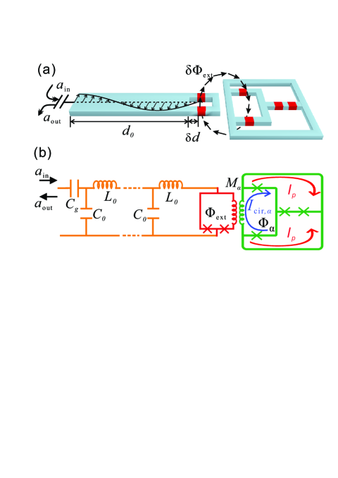
Figure 1: (a) Schematic and (b) lumped circuit diagrams of a SQUID-terminated $\lambda/4$ resonator interacting with a gradiometric four-Josephson-junction flux qubit Paauw et al. (2009) via the mutual inductance $M_{\alpha}$. This interaction is due to NPDC as follows: $I_{\text{cir},\alpha}$ (related to the qubit operator $\sigma_{z}$) generates a flux perturbation on the bias flux $\delta\Phi_{\text{ext}}$, which in turn changes the effective length $d_{0}$ of the resonator by an amount $\delta d$. The result is a dispersive interaction where the photon-number operator $a^{\dagger}a$ couples to the qubit-state operator $\sigma_{z}$. The resonator capacitance and inductance per unit length are $C_{0}$ and $L_{0}$, respectively. The red bars in (a) and crosses in (b) represent the Josephson junctions. To dispersively readout the qubit state, one can apply an input field $a_{\text{in}}$ via the capacitance $C_{g}$. The output field is denoted by $a_{\text{out}}$.

Both the SQUID nonlinear inductance $L_{s}(\Phi_{\text{ext}})$ and the capacitance $C_{s}$ are much smaller than the total capacitance $C_{t}=d_{0}C_{0}$ and inductance $L_{t}=d_{0}L_{0}$ of the resonator. Based on a distributed-element model and its boundary conditions (see Appendix B), the resonator fundamental mode is of quarter-wavelength ($\lambda/4$) and its eigenfrequency depends on the SQUID nonlinear inductance $L_{s}(\Phi_{\text{ext}})$, and can be tuned via $\Phi_{\text{ext}}$ according to the following relations:

$$\omega_{r0}=\omega_{0}\left[1-\frac{L_{s}(\Phi_{\text{ext}}^{0})}{L_{t}}\right],$$ (3a)

$$R=\frac{\partial\omega_{r}}{\partial\Phi_{\text{ext}}}\Big{|}_{\Phi_{\text{ext}}^{0}}=-\frac{\pi\omega_{0}L_{s}(\Phi_{\text{ext}}^{0})}{\Phi_{0}L_{t}}\tan\left(\frac{\pi\Phi_{\text{ext}}^{0}}{\Phi_{0}}\right),$$ (3b)

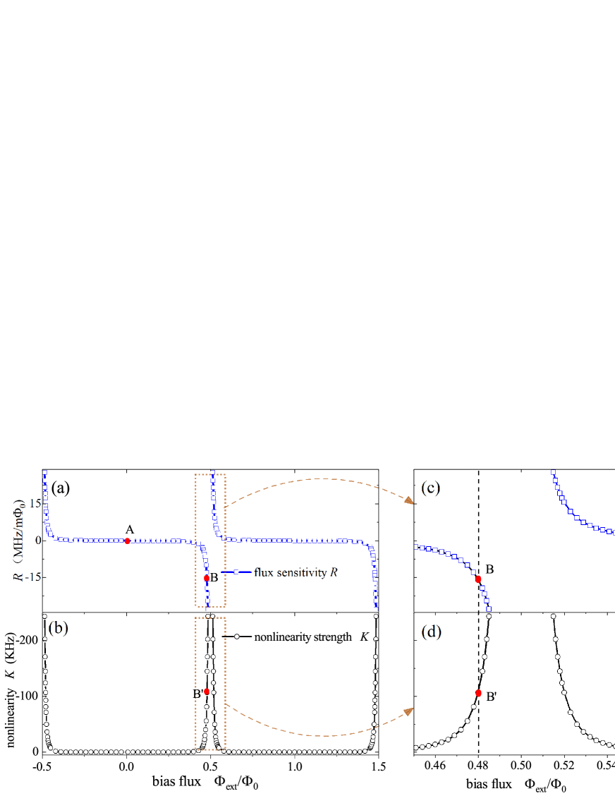
Figure 2: (a) Resonator flux sensitivity $R$ and (b) its Kerr nonlinearity $K$ versus the SQUID flux bias $\Phi_{\text{ext}}$. Parameters are adopted from the experiments in Ref. Pogorzalek et al. (2017); Eichler and Petta (2018): $\omega_{0}/(2\pi)=6~{}\text{GHz}$, $E_{s}/(2\pi)=2.5~{}\text{THz}$ and $L_{r}=10~{}\text{nH}$. Point A (B) corresponds to the qubit-resonator decoupling (coupling) regime. (c) and (d) are, respectively, the local enlarged plots of (a) and (b) in the range $\Phi_{\text{ext}}\in[0.45,0.55]$.

where we assume that the external flux $\Phi_{\text{ext}}$ is composed of a prebiased static part $\Phi_{\text{ext}}^{0}$ and a small deviation part $\delta\Phi_{\text{ext}}\ll\Phi_{\text{ext}}^{0}$. Similar to the discussions in Ref. Johansson et al. (2014) and its experimental realization in Ref. Eichler and Petta (2018), this parametric boundary condition changes the resonator effective length $d_{0}$ slightly, which is akin to a moving mirror for modulating the effective wavelength in the optomechanical system. Note that $R$ is the sensitivity of the frequency $\omega_{r}$ tuned by the external flux $\Phi_{\text{ext}}$, and $\omega_{r0}$ is the renormalized mode frequency. As discussed in Refs. Wallquist et al. (2006); Bourassa et al. (2012); Eichler and Wallraff (2014), the attached SQUID introduces a Kerr nonlinearity ($K_{D}$) to the whole circuit, which is proportional to $[L_{s}(\Phi_{\text{ext}})/L_{t}]^{3}$, and approximately given as Eichler and Petta (2018):

$$K_{D}\approx-\frac{\pi e^{2}\omega_{r0}^{2}L_{t}}{8}\left[\frac{\pi L_{s}(\Phi_{\text{ext}})}{2L_{t}}\right]^{3}.$$ (4)

Figure 2 shows the flux sensitivity $R$ and the Kerr nonlinearity $K_{D}$ versus the applied flux $\Phi_{\text{ext}}$. One finds that, when biasing $\Phi_{\text{ext}}$ from zero to $\approx\Phi_{0}/2$, both $|R|$ and $K_{D}$ increase rapidly from zero. This indicates that the SQUID is a highly nonlinear element and can be exploited for enhancing nonlinear couplings. In our proposal, the static flux bias $\Phi_{\text{ext}}^{0}$ is prebiased by an external field, while the flux deviation $\delta\Phi_{\text{ext}}$ is generated by the circulating current $I_{\text{cir},\alpha}$ of the flux qubit. As shown in Appendix D, one can employ the SQUID-terminated resonator to detect the qubit state, and the Hamiltonian for this system becomes

$$H_{\alpha}=\omega_{r}^{\prime}a^{{\dagger}}a+\frac{\omega_{q}}{2}\sigma_{z}+\chi_{z}^{D}\sigma_{z}a^{{\dagger}}a+K_{D}(a^{{\dagger}}a^{{\dagger}}aa),$$ (5)

where $\chi_{z}^{D}=RM_{\alpha}I_{-}$ is the NPDC strength. The identity matrix term in $I_{\text{cir},\alpha}$ only slightly renormalizes the mode frequency as $\omega_{r}^{\prime}=\omega_{r0}+RM_{\alpha}I_{+}$. Note that $H_{\alpha}$ commutes with $\sigma_{z}$, indicating that a qubit readout via $H_{\alpha}$ is not deteriorated by intracavity photons. Apparently, compared with $H_{\text{d}}$ [Eq. (1)] based on the Rabi model, $H_{\alpha}$ has no relation to the dipole-field coupling but results from the circulating current $I_{\text{cir},\alpha}$ of the flux qubit affecting the effective length of the resonator. The Purcell decay and critical measuring photon-number limitation is effectively eliminated. Moreover, we can neglect higher-energy-level transitions, because the described NPDC is induced without dipole-field interactions. As a result, both quantum information processing and qubit-readout fidelities can be improved compared to other methods affected by higher-energy-level transitions. In fact, this is the core mechanism and advantage of the QND readout based on $H_{\alpha}$ in our proposal.

However, in the dispersive-readout experiments, because the readout resonator is a nonlinear circuit element, one cannot inject plenty of photons without any limitation. As discussed in Appendix B, we have assumed that the attached SQUID is approximately a harmonic element, which corresponds to adopting the quadratic approximation for the SQUID potential. We have expanded its cosine potential as a quartic function. This approximation leads to the following critical intracavity photon number:

$$n_{c}=|\alpha_{c}|^{2},\qquad\alpha_{c}=\frac{\Phi_{0}\sqrt{{2\omega_{r}C_{t}}}}{4\pi\cos(\frac{\pi\omega_{r}}{2\omega_{0}})},$$ (6)

above which the dispersive readout process cannot be realized effectively. In Fig. 3, we plotted $n_{c}$ versus the bias flux $\Phi_{\text{ext}}$. The red point corresponds to that in Fig. 2. We find that the critical number decreases quickly when $\Phi_{\text{ext}}\rightarrow 0.5$. This sets an upper bound when employing this circuit layout for the flux qubit readout, as will be discussed in the next section.

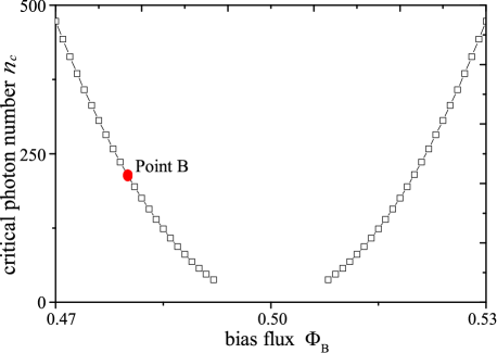
Figure 3: Critical photon number $n_{c}$ versus the bias flux $\Phi_{\text{ext}}$. The red point corresponds to the point B in Fig. 2. The parameters assumed here are the same as those in Fig. 2.

Another advantage of this NPDC-based layout is that the dispersive coupling $\chi_{z}^{I}$ can be switched on/off by tuning $\Phi_{\text{ext}}$. When implementing a gate operation to the qubit, one can bias the flux at $\Phi_{\text{ext}}=N\Phi_{0}$ (where $N$ is an integer, see point A in Fig. 2(a), the flux sensitivity $R$ is zero so $\chi_{z}^{D}=0$. The readout resonator decouples from the qubit and does not disturb quantum information processing. Once a qubit readout is required, one can reset $\Phi_{\text{ext}}$ around $N\Phi_{0}/2$ (point B) to reestablish the coupling, which is fast and only takes several nanoseconds according to Sandberg et al. (2008).

The longitudinal degree of freedom of a flux qubit for quantum information processing was analyzed in, e.g., Richer and DiVincenzo (2016); Richer et al. (2017); Billangeon et al. (2015a, b), including gate operations without Purcell limitations. Another related work Didier et al. (2015a) achieved fast qubit readout via parametric modulation of the longitudinal coupling. Compared with our methods, parametric modulation shifts the qubit frequency in a time-dependent manner with a large amplitude. Moreover, higher-order effects, which are induced by the modulation process, might also destroy the readout fidelity of the system in Didier et al. (2015a). Other two recent papers Ikonen et al. (2019); Touzard et al. (2019) on dispersive coupling are based on a Jaynes-Cummings-type Hamiltonian. Therefore, the Purcell effects (although could be suppressed by the Purcell filters) still exist and limit the qubit-readout fidelity of the systems of Ikonen et al. (2019); Touzard et al. (2019). Compared with these works, our methods can avoid the Purcell effects effectively.

For the qubit, the circulating current difference $I_{-}$ in the $\alpha$-loop is about one order lower than $I_{p}$. At point B in Fig. 2(c) and (d), the flux sensitivity is $|R|/(2\pi)\simeq 16~{}\text{MHz}/(\text{m}\Phi_{0})$ (point B) with a nonlinearity $K_{D}/(2\pi)\simeq 110~{}\text{kHz}$ (point $\rm{B}^{\prime}$). To avoid this Kerr nonlinear effect, one must ensure that $\chi_{z}^{D}\gg K_{D}$.

The mutual inductance between two circuit elements can be (1) geometric, (2) kinetic, and (3) nonlinear Josephson inductance. Usually the geometric inductance is very small. However, the kinetic inductance can be very large by sharing a nanowire between two circuit elements Zhang et al. (2019); Grünhaupt et al. (2018); Niepce et al. (2019). The kinetic inductance increases when decreasing the cross-section area of a nanowire made from aluminum films. To achieve stronger $\chi_{z}^{D}$, one can employ the kinetic mutual inductance $M_{\alpha}$ by sharing a branch of the $\alpha$-loop with the resonator SQUID Paauw (2009); Meservey and Tedrow (1969); Annunziata et al. (2010); Natarajan et al. (2012); Doerner et al. (2018). As discussed in the experimental paper Schwarz (2015), the kinetic inductance per unit length can be $L_{k}=5$ pH/$\mu$m for the cross-sectional area $S=100\times 90\,$nm². Therefore, the value of 15pH can be easily achieved and the NPDC strength is about $\chi_{z}^{D}/(2\pi)\backsimeq 7~{}\text{MHz}$, which is of the same order as the IDC strength reported in experiments Majer et al. (2007); Jeffrey et al. (2014), and strong enough for a qubit QND readout.

Another method is to employ a Josephson junction as a mutual inductance. In Ref. Grajcar et al. (2006), the Josephson inductance was reported as large as 40 pH. In an experimental realization, one can employ a much larger inductance to achieve even much stronger NPDC than that estimated in our paper. Note that the coupling strength $\chi_{z}^{D}$ can still be enhanced by reducing the wire cross-section area of the kinetic inductance, or by inserting a nonlinear JJ inductance at the connecting position Grajcar et al. (2005, 2006).

III Non-perturbative dispersive qubit readout

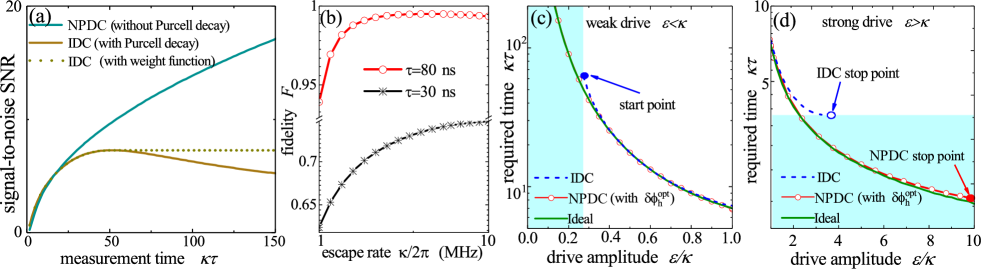
Figure 4: (a) Signal-to-noise ratio for the NPDC- and IDC-based readout mechanisms versus the integrated measurement time $\kappa\tau$. (b) Measurement fidelity $F_{s}$ versus photon escape rate $\kappa$ at $\tau=30~{}\text{ns}$ and $\tau=80~{}\text{ns}$. In (a) and (b) we set $\epsilon=\chi_{z}$. (c, d) The measurement time $\kappa\tau$ required to reach the fidelity $99.99\%$ versus the drive amplitude $\epsilon$ for: (c) weak ($\epsilon/\kappa<1$) and (d) strong ($\epsilon/\kappa\geq 1$) drives. In the IDC readout, the solid (empty) circle marks the start (stop) point, indicating the lower (upper) bound of $\epsilon$. In the NPDC readout, we employ the optimal shifted homodyne angle $\delta\phi_{h}^{\text{opt}}$ for different drive strengths, as discussed in Appendix E. The red solid point is the NPDC stop point due to the nonlinear effects. We set the parameters as: $\lambda=0.1$, $K/(2\pi)=100~{}\text{kHz}$, $\chi_{z}/(2\pi)=8~{}\text{MHz}$, and $\kappa/(2\pi)=16~{}\text{MHz}$. The cyan areas are the regimes that cannot be reached in the IDC-based readout mechanism due to the Purcell effects.

Based on the layout in Fig. 1, one can realize an ideal QND readout of the flux qubit via the coupling Hamiltonian $H_{\alpha}$ without being disturbed by the Purcell effects. To compare the IDC and NPDC readouts of the qubit, below we assume

$$\chi_{z}^{I}=\chi_{z}^{D}=\chi_{z},\quad K_{D}=K_{I}=K.$$ (7)

Applying an incident field $a_{\text{in}}$ in the left port of the resonator at the resonator frequency $\omega_{r}^{\prime}$, the quantum nonlinear Langevin equation for the resonator operator reads

$$\frac{da(t)}{dt}=-i\chi_{z}\sigma_{z}a(t)-2iK\langle N(t)\rangle a(t)-\frac{1}{2}\kappa a(t)-\sqrt{\kappa}a_{\text{in}}(t).$$ (8)

For the IDC readout, $\langle N(t)\rangle=\langle n(t)\rangle\sigma_{z}$ is due to the qubit-dependent Kerr nonlinearity, where $\langle n(t)\rangle=\langle a^{{\dagger}}(t)a(t)\rangle$ is the average intracavity photon number. For the NPDC-based readout mechanism, $\langle N(t)\rangle=\langle n(t)\rangle$ results from the standard Kerr term. This input field $a_{\text{in}}(t)=\alpha_{\text{in}}+d_{\text{in}}(t)$ is characterized by its mean value (a coherent drive) $\alpha_{\text{in}}=-\epsilon e^{i\theta_{d}}/\sqrt{\kappa}$ and fluctuation $d_{\text{in}}(t)$. Due to the dispersive coupling, the qubit state is encoded in the output quadrature $Y(\phi_{h})=a_{\text{out}}^{{\dagger}}e^{i\phi_{h}}+a_{\text{out}}e^{-i\phi_{h}}$. The measurement corresponds to a homodyne detection of $Y(\phi_{h})$ with an integration time $\tau$, i.e.,

$$M(\tau)=\sqrt{\kappa}\int_{0}^{\tau}Y(\phi_{h})dt.$$ (9)

We first consider an ideal readout with $K=0$. By formally integrating Eq. (8) and using the input-output relation $a_{\text{out}}=\sqrt{\kappa}a+a_{\text{in}}$, we obtain the separation signal $M_{s}=\langle M_{s}\rangle_{|e\rangle}-M_{s,|g\rangle}$ (with $\langle\sigma_{z}\rangle=\pm 1$) as

$$M_{s}(\tau)=4\epsilon\sin{2\theta_{q}}\sin(\theta_{d}-\phi_{h})$$

$$\times\left[\tau-\frac{4\cos^{2}(\theta_{q})}{\kappa}\left(1-\frac{\sin(\chi_{z}\tau+2\theta_{q})}{\sin(2\theta_{q})}e^{-\frac{1}{2}\kappa\tau}\right)\right],$$ (10)

where $\theta_{q}=\arctan({2\chi_{z}/\kappa})$ is the rotating angle of the output field. We integrated the Langevin equation in (E2), to obtain Eq. (E3), which shows the coherent amplitudes $\alpha$ of the intracavity field. In our derivation, we approximately used the classical part of the intracavity field operator to describe the photon number, i.e., $\langle n(t)\rangle=|\alpha(t)|^{2}$. As derived in Appendix E, $\langle n(t)\rangle$ is given by

$$\langle n(t)\rangle = \left(\frac{2\epsilon}{\kappa}\right)^{2}\cos(\theta_{q})\bigg{[}1+\exp(-\kappa t)$$ (11)

$$- 2\cos(\chi_{z}\langle\sigma_{z}\rangle t)\exp\left(-\frac{1}{2}\kappa t\right)\bigg{]}.$$

In the steady state ($\kappa t\gg 1$), the intracavity photon number is $n\backsimeq(2\epsilon/\kappa)^{2}\cos(\theta_{q})$. The fluctuation $d_{\text{out}}(t)$ introduces noise into the measurement signal. For the vacuum input, the noise reads Didier et al. (2015b)

$$M_{N}^{2}(\tau)=[\langle M_{N}^{2}(\tau)\rangle_{|e\rangle}+\langle M_{N}^{2}(\tau)\rangle_{|g\rangle}]=2\kappa\tau.$$ (12)

In the long-time limit $\kappa\tau\gg 1$, the signal-to-noise-ratio $\mathcal{R}=M_{s}(\tau)/M_{N}(\tau)$ is optimized by setting $\theta_{d}-\phi_{h}=\pi/2$ and $\theta_{q}=\pi/4$ (i.e., $\chi_{z}=\kappa/2$). The measurement fidelity is defined as

$$F_{m}=\frac{1+\text{erf}(\mathcal{R}/2)}{2},$$ (13)

where $\text{erf}(x)$ is the error function.

As discussed in Appendix E, the effects of the nonlinearities in the IDC and NPDC readouts are different: the Kerr nonlinearity in the IDC readout is qubit-dependent, and symmetrically reduces the effective cavity pull Boissonneault et al. (2008), which causes a poor signal separation if $\langle a^{{\dagger}}(t)a(t)\rangle$ is large. For the NPDC readout, $K$ leads to asymmetric rotation angles of the cavity field in the phase space. However, the signal-separation distance is still high, even for large $\langle a^{{\dagger}}(t)a(t)\rangle$. Moreover, for the IDC-based readout mechanism, because $[H_{x},\sigma_{z}]\neq 0$, $H_{\text{d}}$ is not an ideal QND readout Hamiltonian. There is a qubit Purcell decay channel $\Gamma_{p}$ via the readout resonator, which is proportional to the photon escape rate $\kappa$. Assuming the qubit relaxation is limited by the Purcell decay, the readout $\mathcal{R}$ can be numerically derived by replacing $\sigma_{z}$ by

$$\langle\sigma_{z}\rangle(t)=[1+\langle\sigma_{z}\rangle(0)]\exp(-\Gamma_{p}t)-1$$ (14)

in Eq. (8). It is hard to obtain analytical results of Eq. (8) by including both $K$ and $\Gamma_{p}$. Thus, below we present only numerical results Johansson et al. (2012, 2013). We first plot the signal-to-noise-ratio versus time in Fig. 4(a). In the IDC readout, due to the Purcell decay, the signal-to-noise-ratio decreases after reaching its maximum. In our simulations, the separation signal $M_{s}$ indeed saturates at a constant level when increasing the measurement time. However, in Fig. 4(a), we plot the signal-to-noise-ratio, which is defined as $\mathcal{R}=M_{s}/\sqrt{2\kappa\tau}$. By increasing the measurement time $\tau$, the signal separation $M_{s}$ finally reaches its steady value, while a homodyne detector continuously collects the input noise. Therefore, in our discussions, $\mathcal{R}$ decreases with time as shown in Fig. 4(a). Note that our definition is different from that in the experimental works Gambetta et al. (2007); Bultink et al. (2018); Heinsoo et al. (2018). The weight function $W(t)$ determines how much of the signal power is integrated at time $t$. This function $W(t)$ can, in principle, be chosen a square (boxcar) function or can be optimized based on certain experimental implementations Bultink et al. (2018). In Fig. 4(a), we use a simple square function, which leads to a constant value of $\mathcal{R}$ after reaching its highest point.

For the NPDC readout, the escaping photon does not lead to the decay of the qubit states, and $\mathcal{R}$ is proportional to $\sqrt{2\kappa\tau}$ in the long-time limit $\kappa\tau\gg 1$ Didier et al. (2015a, b). One may try to suppress $\Gamma_{p}$ by reducing $\kappa$. However, to achieve a fast qubit readout, $\kappa$ should be large enough to allow readout photons to escape quickly. The relation can be clearly found in Fig. 4(b): for a certain integrated time $\tau$, the readout fidelity increases with $\kappa$. Therefore, to reduce the Purcell decay, one should decrease the measurement speed with a relatively low $\kappa$ in the IDC readout. However, this trade-off relation does not exist in the NPDC readout: it is without dipole-field coupling, and the qubit QND readout is not disturbed by the Purcell decay. One can employ a large $\kappa$ to speed up the readout.

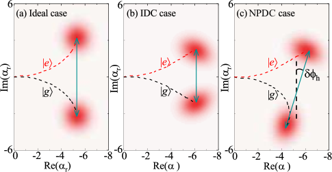
Figure 5: The Wigner distributions of the intracavity field for (a) the ideal, (b) IDC, and (c) NPDC readouts for the same measurement time $\kappa\tau=3$. The red (black) curves are the time-dependent evolution trajectories in phase space, and the upper (lower) signals correspond to the qubit being in its excited (ground) state. The arrows represent signal separation distances and directions. The parameters adopted here are the same as those in Fig. 4(d), and the drive strength is assumed to be the same as for the stop point. For the NPDC readout in (a), the signal separation direction is rotated by an angle $\delta\phi_{h}$.

As shown in Fig. 5 (with the same measurement time $\kappa\tau=3$), one can find that the Wigner functions for the IDC- and NPDC-based readout mechanisms are not perfectly symmetric Gaussian functions. This is due to the Kerr nonlinearity, which modifies the coherent state of the resonator field. Consequently, the collected noise in the homodyne measurement for a given quadrature direction in phase space can be different from the ideal result given in Eq. (12) assuming a classical resonator field. Nevertheless, we employ the Heisenberg-Langevin equation and treat the resonator field to be classical in Fig. 4. Precise numerical calculations of the evolution of our system, including the quantized resonator field with many injected photons, require to assume the Hilbert-space dimension of the order of about hundreds and, thus, require time-consuming numerical calculations. However, for the parameters considered in our manuscript, treating the resonator field to be coherent leads only to very small difference, compared to the fully quantum treatment of the entire system.

To verify this classical approximation of the resonator field, we plotted Fig. 6 by applying the quantum treatment of the resonator field for the parameters at the IDC stop point in Fig. 4(d). This figure shows the effect of the quantum noise $M_{N}(\tau)$ changing with the measurement time for the ideal, NPDC, and IDC readouts. The vertical lines correspond to the required time for the IDC and NPDC readouts in Fig. 4(d), respectively, where the noise shift, which is induced by the Kerr effect, is negligible compared to the ideal readout and one can employ our analytical results given in Eq. (12) to calculate $\mathcal{R}$. If one insists on achieving a higher fidelity, the required time becomes longer and, thus, one should calculate the input quantum noise changing with the measurement time for different methods in the fully quantum treatment of the resonator field. Moreover, by comparing the IDC and NPDC results in the long-measurement-time limit ($\kappa\tau\gg 1$), we find that the noise for the NPDC readout increases more slowly compared to the noise in the IDC readout. This is another advantage of our proposal.

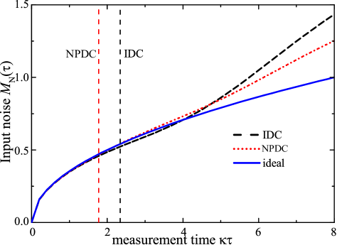
Figure 6: The measurement noise $M_{N}(\tau)$ for the ideal, IDC, and NPDC readouts obtained by quantum simulations. The dashed lines correspond to the required measurement time for the IDC and NPDC proposals. Parameters assumed here are the same as those for the stop point of the IDC readout shown in Fig. 4(d).

In Figs. 4(c) and 4(d), we plot the time $\kappa\tau$ required to reach the fidelity $99.99\%$ as a function of the drive strength $\epsilon$. Figure 4(c) corresponds to the weak-drive limit ($\epsilon<\kappa$). Due to the qubit Purcell decay, there is a lower limit of $\epsilon_{\text{min}}$ (start point) for the drive amplitude in the IDC readout. If $\epsilon<\epsilon_{\text{min}}$ (cyan area), the measurement can never reach the desired fidelity even if taking an infinitely-long time. However, for the NPDC readout (red dotted curve) based on our proposal, the ideal fidelity can be reached in principle for $\epsilon<\epsilon_{\text{min}}$.

We should recall that for the NPDC-based readout mechanism, we cannot increase the photon number due to some limitations of Eq. (6). In Fig. 4(d), we marked the corresponding stop point (due to $n_{c}$) for the NPDC readout (red solid point), which is around $\epsilon/\kappa\simeq 10$ and far from the stop point of the IDC readout. Note that the critical photon number $n_{c}$ decreases when the flux bias $\Phi_{\text{ext}}$ is close to $\Phi_{0}/2$. As shown in Fig. 2, there is a trade-off relation between the flux sensitivity $R$ (i.e., the NPDC coupling strength) and $n_{c}$, which might be one of the obstacles for achieving much shorter readout times. In future studies, to reach the minimum readout time, one can optimize the parameters of the whole readout circuits.

In the strong-drive limit, $\epsilon>\kappa$ [Fig. 4(d)], for both two readout mechanisms, the required time $\kappa\tau$ is significantly reduced. Unfortunately, the IDC-based readout mechanism encounters another two Purcell limitations: First, the effective cavity pull is significantly reduced as

$$|\xi_{I}|=\left|\chi_{z}\left(1-\frac{\langle n(t)\rangle}{2n_{c}}\right)\right|,\\$$ (15)

which leads to a reduction of the signal separation. By comparing Fig. 5(a) and (b), it can be found that, for the IDC readout, the signal separation distance (oliver arrows) in phase space is much smaller than that in the ideal readout. Consequently, the required time becomes much longer than that for the ideal readout. Second, to avoid photon-induced qubit-error transitions, the intracavity photon number should be much smaller than the critical photon number $n_{c}=1/(4\lambda^{2})$. This sets another upper bound limitation $\epsilon_{\text{max}}=\kappa/(2\sqrt{2}\lambda)$ for the drive strength Blais et al. (2004). The measurement time $\tau$ cannot be shortened below the stop point.

For large $\langle n(t)\rangle$, the Kerr nonlinearity in the NPDC-based readout mechanism also induce apparent effects. However, as shown in Fig. 5, its main effect is to change the signal separation direction with a small angle $\delta\phi_{h}$ Eichler and Wallraff (2014), while the signal separation distance is still large compared with the IDC readout. Moreover, intracavity photons do not cause qubit-state error flips and, therefore, in principle, there is no such a stop point due to the Purcell effects. To minimize the Kerr effects, we can slightly shift the homodyne angle $\phi_{h}$ by an optimized small angle $\delta\phi_{h}^{\text{opt}}$. The detailed method about how to shift the measurement angle can be found in Appendix E. As seen in Fig. 4(d), the required time can be quite close to the ideal readout. Therefore, by injecting many photons, the measurement time can go far below the Purcell-effect regime.

IV Discussions

IV.1 Multiqubit readout via a single resonator

It is also possible to employ an array of SQUIDs to terminate the measurement resonator (see Ref. Sandberg et al. (2008)). As discussed in Appendix B, the effective nonlinear inductance of each SQUID can be tuned independently via the flux $\Phi_{\text{ext},j}$ produced by an individual flux-bias line. Considering the $j$th SQUID interacting with the $j$th flux qubit ($\sigma_{z,j}$) via its circulating current $I_{\text{cir},\alpha j}$, the interaction Hamiltonian is

$$H_{\alpha,\Sigma}=\sum_{j}\chi_{z,i}\sigma_{z,j}a^{{\dagger}}a,\quad\chi_{z,i}=R(\Phi_{\text{ext},j})I_{\text{cir},\alpha j}M_{j},$$ (16)

with $M_{j}$ being the mutual inductance. To readout the $m$th qubit without being disturbed by other qubit-resonator couplings, one can tune $R(\Phi_{\text{ext},j})$ to zero with $\Phi_{\text{ext},j}=0$ for $j\neq m$, while keeping $R(\Phi_{\text{ext},m})$ around point B (see Fig. 2). In this case, the resonator is employed as a shared readout resonator for each individual qubit. Moreover, we could realize a joint readout of multiqubit states Majer et al. (2007). For the example of two qubits, we set $\chi_{z,1}/2=\chi_{z,2}=\chi_{0}$. The two-qubit basis $\{|e,e\rangle,|e,g\rangle,|g,e\rangle,|g,g\rangle\}$ corresponds to four different rotation angles (in phase space) $\theta_{qN}=\arctan({N\chi_{0}/\kappa})$, with $N=\pm 1,\pm 3$ for the output field, which represents four separated pointer states. This multi-SQUID layout enables scalability for an ideal qubit-joint QND readout.

By assuming similar values of the flux sensitivity $R(\Phi_{\text{ext},j})$ of all the SQUIDs (labeled by the index $j$), the phase drops across each SQUID are also similar Eichler and Wallraff (2014). Due to this property, the Kerr nonlinearity $K^{\prime}_{D}$ increases linearly with the SQUID number $n$, i.e., $K^{\prime}_{D}=nK_{D}$. In all our discussions, the Kerr nonlinearity always decreases the readout fidelity. Therefore, this scalable proposal works well when considering only several SQUIDs and a weak drive field. Beyond these regimes, we should find better proposals for such a qubit-QND readout.

IV.2 Dynamical range of the SQUID-terminated resonator

Finally, we want to discuss the dynamical range of the measurement SQUID-terminated resonator. The differential equation (8) for NPDC readout is nonlinear, and the steady-state solution for the intracavity-photon number can be solved from a cubic equation. To analyze this problem, we need to define the dimensionless effective detuning as

$$\delta^{s}=\frac{\chi_{z}^{D}}{\kappa}\langle\sigma_{z}\rangle,\qquad\delta^{s}\in\left[-\left|\frac{\chi_{z}^{D}}{\kappa}\right|,\left|\frac{\chi_{z}^{D}}{\kappa}\right|\right].$$ (17)

As derived in Ref. Eichler and Wallraff (2014), the critical detuning is $\delta^{s}_{\text{crt}}=-\sqrt{3}/2$, below which the cubic equation might have three solutions for the intracavity-field intensity. Both, the smallest and the largest solutions, are stable for the whole system. However, the intermediate one is unstable, around which the field in the readout resonator might bifurcate. During the dispersive readout, better for the system to avoid this highly nonlinear regime.

As shown Fig. 4(b), a rapid photon escaping rate $\kappa$ improves the readout fidelity. In an experimental implementation, by adopting a large $\kappa$, the dimensionless detuning $|\delta^{s}|$ is a small parameter. For example, in Figs. 4(c) and (d), we adopt $\delta^{s}\in[-1/2,1/2]$, which is out of the bistable regime. Therefore, our proposal can effectively avoid bistability problems induced by the Kerr nonlinearity.

V Conclusions

We showed how to realize an ideal QND readout of a flux qubit via its non-perturbative dispersive coupling with a SQUID-terminated measurement qubit. The coupling can be conveniently switched on and off via an external flux control. Compared with the conventional induced dispersive coupling based on the Rabi model, this mechanism is free of dipole-field interactions and, therefore, it is not deteriorated by the Purcell effects. We can employ a strong drive field and a quick photon escape rate. Thus, both measurement fidelity and speed can avoid the Purcell limitations. Considering a single resonator, which is terminated by a series of SQUIDs, this proposal is scalable and tunable to realize a multi-qubit joint QND readout. In future studies, this proposed method might be developed to include a weak continuous measurement to monitor the superconducting flux qubit Groen et al. (2013); Tan et al. (2015). Moreover, this method can be applied to other weak-signal measurements, such as detecting virtual photons or qubit-excited states in the ultrastrong light-matter coupling regime Cirio et al. (2017); Kockum et al. (2018).

VI acknowledgments

The authors acknowledge fruitful discussions with Xiu Gu, Yu-Xi Liu, Zhi-Rong Lin, and Wei Qin. X.W. thanks Yun-Long Wang for helping to depict the schematic diagrams. X.W. is supported by China Postdoctoral Science Foundation No. 2018M631136, and the Natural Science Foundation of China under Grant No. 11804270. A.M. and F.N. acknowledge the support of a grant from the John Templeton Foundation. F.N. is supported in part by the: MURI Center for Dynamic Magneto-Optics via the Air Force Office of Scientific Research (AFOSR) (FA9550-14-1-0040), Army Research Office (ARO) (Grant No. Grant No. W911NF-18-1-0358), Asian Office of Aerospace Research and Development (AOARD) (Grant No. FA2386-18-1-4045), Japan Science and Technology Agency (JST) (via the Q-LEAP program, and the CREST Grant No. JPMJCR1676), Japan Society for the Promotion of Science (JSPS) (JSPS-RFBR Grant No. 17-52-50023, and JSPS-FWO Grant No. VS.059.18N), and the RIKEN-AIST Challenge Research Fund.

Note added: After posting the e-print of this work in the arXiv Wang et al. (2018), the work by Dassonneville et al. on the same topic was posted in the arXiv R. Dassonneville (2019). That paper describes a protocol very similar to ours, but for a different type of a superconducting qubit, which can be viewed as an experimental realization of the QND measurements of superconducting qubit via non-perturbative dispersive coupling. Those studies indicate that the concept of a QND readout via the NPDC mechanism is experimentally feasible and can receive much more attention, both theoretical and experimental, in the near future.

APPENDICES

Appendix A Induced dispersive coupling and Purcell decay

In a typical system based on superconducting quantum circuits, the conventional light-matter dispersive coupling is based on dipole-field interactions. In the large-detuning regime $g_{x}\ll\Delta_{d}=\omega_{q}-\omega_{a}$ (where $\omega_{q}$ and $\omega_{r}$ are the qubit and resonator frequency, respectively), the system Hamiltonian is approximately described by the Jaynes-Cummings (JC) Hamiltonian

$$H_{R0}=\frac{\omega_{q}}{2}\sigma_{z}+\omega_{r}a^{{\dagger}}a+g_{x}(a\sigma_{+}+a^{{\dagger}}\sigma_{-}).$$ (A1)

In a qubit dispersive readout, one often injects many photons into the resonator to speed up such measurement. Once the photon number is large, it is necessary to push the dispersive coupling into higher-order nonlinear terms. Here we follow the approaches in Refs. Boissonneault et al. (2008, 2009), and derive a more exact nonlinear dispersive coupling Hamiltonian. We first define the unitary transformation $U_{D}$ as Boissonneault et al. (2009):

$$U_{D} = \exp\left\{-\Theta(N_{J})(a^{{\dagger}}\sigma_{-}-a\sigma_{+})\right\},\qquad$$

$$\Theta(N_{J}) = -\frac{\arctan(2\lambda\sqrt{N_{J}})}{2\sqrt{N_{J}}},$$ (A2)

where

$$\lambda=g_{x}/(\Delta_{d}),\quad\Delta_{d}=\omega_{q}-\omega_{r},$$

and

$$N_{J}=a^{{\dagger}}a+|e\rangle\langle e|$$

is a function of the total excitation number operator of the system. Applying the transformation $U_{D}$ to the JC Hamiltonian $H_{R0}$, the off-diagonal terms can be eliminated, and yielding

$$H_{R0}=\frac{\omega_{q}}{2}\sigma_{z}+\omega_{r}a^{{\dagger}}a-\frac{\Delta_{d}}{2}\left(1-\sqrt{1+4\lambda^{2}N_{J}}\right)\sigma_{z}.$$ (A3)

This equation is still the exact diagonalized solution for the system Hamiltonian without any approximation. To obtain the dispersive coupling, we can expand $\sqrt{1+4\lambda^{2}N_{J}}$ to second order in $4\lambda^{2}N_{J}$ to find Boissonneault et al. (2009)

$$H_{R0} = \omega_{r}^{\prime}a^{{\dagger}}a+\frac{\omega_{q}}{2}\sigma_{z}$$ (A4)

$$+\chi_{z}^{I}a^{{\dagger}}a\sigma_{z}+K_{I}(a^{{\dagger}}a^{{\dagger}}aa)\sigma_{z},$$

where $\omega_{r}^{\prime}$ is the shifted resonator frequency,

$$\chi_{z}^{I}=g_{x}^{2}(1-2\lambda^{2})/\Delta_{d}\backsimeq g_{x}^{2}/\Delta_{d}$$

is the IDC strength, and

$$K_{I}=-g_{x}^{4}/\Delta_{d}^{3}$$

is the qubit-dependent Kerr nonlinearity strength. Note that the validation of this perturbation result requires that Eq. (A4) does not only depend on a small parameter $\lambda\ll 1$, but also requires that the total excitation number satisfies $\langle N_{J}\rangle\ll 1/(4\lambda^{2})$, which results in a critical photon $n_{c}=1/(4\lambda^{2})$ Blais et al. (2004). In a qubit measurement, the intracavity photon number should be much smaller than $n_{c}$.

The coupling Hamiltonian between the measurement and the environment is

$$H_{\kappa}=\int_{0}^{\infty}\sqrt{\kappa(\omega)}[b^{{\dagger}}(\omega)+b(\omega)](a+a^{{\dagger}})d\omega,$$

where $b(\omega)$ is the annihilation operator of the environmental mode $\omega$. Applying the unitary transformation $U_{D}$ to the field operators $(a+a^{{\dagger}})$, we obtain

$$U_{D}^{{\dagger}}(a+a^{{\dagger}})U_{D}\simeq(a+a^{{\dagger}})+\lambda(\sigma_{-}+\sigma_{+})+O^{\prime}(\lambda^{2}).$$ (A5)

One can find that the field operator acquires an extra part related to the qubit operators $\sigma_{\pm}$ in the dressed basis. In the interaction picture and applying the rotating-wave approximation to the Hamiltonian $H_{\kappa}$, we obtain

$$H_{\kappa} = \int_{0}^{\infty}d\omega\sqrt{\kappa(\omega)}[b(\omega)a^{{\dagger}}e^{-i(\omega-\omega_{r})t}+\text{H.c.}]$$ (A6)

$$+ \!\lambda\!\int_{0}^{\infty}d\omega\sqrt{\kappa(\omega)}[b(\omega)\sigma_{+}e^{-i(\omega-\omega_{q})t}+\text{H.c.}],$$

where the last term describes an additional Purcell decay channel for the qubit. The cavity is assumed to couple with a thermal environment with zero average boson number. Following the standard steps of deriving the master equation, we find that the last term adds an extra qubit decay with rate $\Gamma_{p}=\lambda^{2}\kappa(\omega_{q})$. In this work, we assume that $\kappa(\omega_{q})$ is not frequency dependent and equals to the photon escape rate $\kappa$.

Appendix B SQUID-terminated transmission line resonator

B.1 Tuning the resonator frequency via SQUID: Linear approximation

As shown in Fig. 1, we consider a transmission line resonator (TLR) (along the $x$ axis with length $d_{0}$) short-circuited to ground by terminating its right side with a dc SQUID (at the position $x=d_{0}$) Wallquist et al. (2006); Johansson et al. (2009). The two Josephson junctions of the SQUID are assumed to be symmetric with identical Josephson energy $E_{s0}$ and capacitance $C_{s}$. The effective Josephson energy of the SQUID is tuned with the external flux $\Phi_{\text{ext}}$, according to the relation $E_{s}=2E_{s0}|\cos(\pi\Phi_{\text{ext}}/\Phi_{0})|$ ($\Phi_{0}$ is the flux quantum). For an asymmetric SQUID with two different Josephson energies $E_{s1}$ and $E_{s2}$, the effective Josephson energy of the SQUID is given by

$$E^{\prime}_{s}=E_{\Sigma}\sqrt{\cos^{2}\left(\frac{\pi\Phi_{\text{ext}}}{\Phi_{0}}\right)+d_{0}\sin^{2}\left(\frac{\pi\Phi_{\text{ext}}}{\Phi_{0}}\right)},$$ (B1)

where

$$d_{0}=\frac{E_{s1}-E_{s2}}{E_{s1}+E_{s2}},$$ (B2)

is the junction asymmetric parameter. From Eq. (B1), the asymmetric effects can be neglected under the condition

$$d_{0}<\cot\left(\frac{\pi\Phi_{\text{ext}}}{\Phi_{0}}\right).$$ (B3)

In our work, we consider $\Phi_{\text{ext}}/\Phi_{0}\in[0.46,0.48]$, which results $d_{0}<7\%$. The present fabrication technology can control the junction asymmetric parameter within $d_{0}<2\%$. Therefore, the condition in Eq. (B3) is within reach of current experiments Gu et al. (2017).

Note that the SQUID has a nonlinear inductance

$$L_{s}(\Phi_{\text{ext}})=\frac{\Phi_{0}^{2}}{(2\pi)^{2}E_{s}(\Phi_{\text{ext}})}$$

and its Lagrangian is written as Sandberg et al. (2008); Wallquist et al. (2006)

$$\mathcal{L}=\sum_{i=1,2}\left(\frac{\Phi_{0}^{2}C_{s}}{2(2\pi)^{2}}\dot{\phi_{i}}^{2}+E_{s0}\cos{\phi_{i}}\right).$$ (B4)

Setting $\phi_{+}=(\phi_{1}+\phi_{2})/2$ and $\phi_{-}=(\phi_{1}-\phi_{2})/2=\pi\Phi_{\text{ext}}/\Phi_{0}$, we rewrite Eq. (B4) as

$$\mathcal{L}=\frac{\Phi_{0}^{2}C_{s}}{(2\pi)^{2}}\dot{\phi}_{+}^{2}+E_{s}\cos{\phi_{+}}.$$ (B5)

Given that $E_{s}\gg(2e)^{2}/(2C)$, the zero-point fluctuation in the plasma oscillation is of small amplitude with $\phi_{z0}=\sqrt[4]{4e^{2}/(2C_{s}E_{s})}\ll 1$, the SQUID is around its quantum ground state Johansson et al. (2014). The SQUID can be seen as a harmonic oscillator with Lagrangian Wallquist et al. (2006)

$$\mathcal{L}\simeq\frac{\Phi_{0}^{2}C_{s}}{(2\pi)^{2}}\dot{\phi}_{+}^{2}-\frac{E_{s}}{2}\phi_{+}^{2}.$$ (B6)

Let us denote the transmission-line capacitance and inductance per unit length as $C_{0}$ and $L_{0}$, respectively. The dynamics of the field along the transmission-line direction (denoted as the $x$ axis) is described by the Helmholtz wave equation

$$\frac{\partial^{2}\psi(x,t)}{\partial t^{2}}-v^{2}\frac{\partial^{2}\psi(x,t)}{\partial x^{2}}=0,$$ (B7)

where $v=1/\sqrt{L_{0}C_{0}}$ is the wave velocity. At $x=0$ with a large capacitance $C_{g}$, the bound condition is $\partial_{x}\psi(0,t)=0,$ which requires that the wavefunction solutions of Eq. (B7) for a mode $k$ have the form $\psi(x,t)=\psi_{0}\sin(kvt)\cos(kx)$. At $x=d_{0}$, the boundary conditions are Wallquist et al. (2006); Johansson et al. (2010):

$$\psi(d_{0},t)=\phi_{+}(t),$$

$$2C_{s}\ddot{\psi}(d_{0},t)+\frac{(2\pi)^{2}}{\Phi_{0}^{2}}E_{s}\psi(d_{0},t)+\frac{\partial_{x}\psi(d_{0},t)}{L_{0}}=0.$$ (B8)

By substituting the wave function into Eq. (B8), one can find that the mode frequency $\omega_{r}=vk$ of the resonator can be derived from the following transcendental equation Pogorzalek et al. (2017):

$$\frac{\pi\omega_{r}}{2\omega_{0}}\tan\!\!\bigg{(}\frac{\pi\omega_{r}}{2\omega_{0}}\bigg{)}=\frac{(2\pi)^{2}}{\Phi_{0}^{2}}L_{t}E_{s}(\Phi_{\text{ext}})-\frac{2C_{s}}{C_{t}}\bigg{(}\frac{\pi\omega_{r}}{2\omega_{0}}\bigg{)}^{2},$$ (B9)

where $L_{t}=d_{0}L_{0}$ and $C_{t}=d_{0}C_{0}$ are the total inductance and capacitance of the resonator, respectively. The fundamental frequency of the quarter-wavelength resonator is $\omega_{0}=\pi v/(2d_{0})$. By assuming that the capacitances of the Josephson junctions $C_{s}$ are much smaller compared with the total capacitance $C_{t}$, we neglect the last term in Eq. (B9). Because the total inductance $L_{t}$ strongly exceeds that of the SQUID nonlinear inductance $L_{s}(\Phi_{\text{ext}})$, we find $\omega_{r}/\omega_{0}\simeq 1$, and rewrite Eq. (B9) as

$$\left[\frac{\pi\omega_{r}}{2\omega_{0}}\tan\bigg{(}\frac{\pi\omega_{r}}{2\omega_{0}}\bigg{)}\right]^{-1}=\frac{L_{s}(\Phi_{\text{ext}})}{L_{t}}.$$ (B10)

By expanding the left-hand side of Eq. (B10) with $(\pi\omega_{r})/(2\omega_{0})$ around $\pi/2$ to first order, we obtain

$$\omega_{r}=\omega_{0}\left[1-\frac{L_{s}(\Phi_{\text{ext}})}{L_{t}}\right].$$ (B11)

From this equation, we find that the external flux $\Phi_{\text{ext}}$ through the SQUID determines its nonlinear inductance, which eventually shifts the mode frequency $\omega_{r}$. Similar to the discussions in Ref. Johansson et al. (2010), this parametric bound condition changes the resonator effective length only slightly, which is akin to a moving mirror for modulating the effective wavelength in the optomechanical system. We assume that the external flux is composed of a prebiased static part $\Phi_{\text{ext}}^{0}$ and a small deviation part $\delta\Phi_{\text{ext}}\ll\Phi_{\text{ext}}^{0}$, and write the mode frequency as

$$\omega_{r}=\omega_{r0}+\frac{\partial\omega_{r}}{\partial\Phi_{\text{ext}}}\Big{|}_{\Phi_{\text{ext}}^{0}}\delta\Phi_{\text{ext}},$$ (B12)

where the shifted mode frequency $\omega_{r0}$ and its flux sensitivity $R$ are expressed in Eq. (3). Note that in our discussions we assume that the dc-SQUID loop inductance can be neglected when compared with $L_{s}$, which can be easily satisfied in experiments Eichler and Petta (2018). Therefore, the frequency jump effects of the mode frequency due to its hysteretic flux response can also be neglected Pogorzalek et al. (2017).

B.2 Resonator self-Kerr nonlinearity

Because the SQUID is a nonlinear element, attaching it at the end of the resonator makes the entire system nonlinear. Here we want to estimate the amount of such nonlinearity. In Eq. (B6), we approximately viewed the SQUID as a linear circuit element by neglecting the higher-order terms. To obtain the nonlinear terms of this system, we expand the SQUID cosine potential to include non-quadratic corrections. Because $\phi_{+}\ll 1$, it is enough to consider its forth-order terms in the Lagrangian

$$\mathcal{L}=\frac{\Phi^{2}C_{s}}{(2\pi)^{2}}\dot{\phi}_{+}^{2}-\frac{E_{s}}{2}\phi_{+}^{2}+\frac{E_{s}}{24}\phi_{+}^{4}+\cdots.$$ (B13)

The boundary condition in Eq. (B8) now contains the cubic term,

$$2 C_{s}\ddot{\psi}(d_{0},t)+\frac{\partial_{x}\psi(d_{0},t)}{L_{0}}$$ (B14)

$$+ \frac{(2\pi)^{2}}{\Phi_{0}^{2}}E_{s}(\Phi_{\text{ext}})\left[\psi(d_{0},t)-\frac{1}{6}\psi^{3}(d_{0},t)\right]\!=0.$$

The cubic term not only relates the boundary equation with both first and third-harmonic modes, but also produces a shift of the resonant frequency, which depends on the photon number of the resonator mode. Comparing Eq. (B14) with Eq. (B8), we can roughly view the Josephson energy $E_{1}(\Phi_{\text{ext}})$ to be slightly modified as

$$E_{1}(\Phi_{\text{ext}})\rightarrow E_{1}(\Phi_{\text{ext}})[1-\frac{1}{6}\psi^{2}(d_{0},t)],$$

which indicates that the nonlinear inductance $L_{s1}(\Phi_{\text{ext}})$ now depends on the intracavity field intensity $\psi^{2}(d_{0},t)$. Employing Eq. (B11), and similar with the deviation in Ref. Eichler and Wallraff (2014), the quantized Hamiltonian of the fundamental mode with the self Kerr nonlinearity can be approximately written as

$$H=\omega_{r0}a^{{\dagger}}a+K_{D}a^{{\dagger}}a^{{\dagger}}aa,$$ (B15)

with the Kerr nonlinearity strength

$$K_{D} = -\frac{\cos^{4}(\frac{\pi\omega_{r}}{2\omega_{0}})}{4L_{s}(\Phi_{\text{ext}})}\left(\frac{2\pi\phi_{zpf}^{2}}{\Phi_{0}}\right)^{2}$$ (B16)

$$\approx -\frac{\pi e^{2}\omega_{r0}^{2}L_{t}}{8}\left[\frac{\pi L_{s}(\Phi_{\text{ext}})}{2L_{t}}\right]^{3},$$

where the quantized form of the field amplitude is

$$\psi_{1}(t)=\phi_{\text{zpf}}\left[a\exp(-i\omega_{r0}t)+a^{\dagger}\exp(i\omega_{r0}t)\right],$$

with

$$\phi_{\text{zpf}}=\frac{2\pi}{\Phi_{0}}\sqrt{\frac{1}{2\omega_{r0}C_{t}}}$$

being the zero-point fluctuations of the flux field Wallquist et al. (2006). The self-Kerr nonlinearity is due to attaching the SQUID at the end the resonator. In our discussion, the condition $L_{s}(\Phi_{\text{ext}})/L_{t}\ll 1$ is always valid, and the Kerr strength $K_{D}$ is proportional to the cubic-order of the small parameter $L_{s}(\Phi_{\text{ext}})/L_{t}$, which is much weaker than the first-order effects [Eq. (B11)]. In the following discussions, we consider this Kerr nonlinearity effects on the qubit readout process.

We also need to check the validity of the quartic expansion approximation in Eq. (B13), which requires $\phi_{+}<1$. Considering the boundary condition in Eq. (B8), one finds that the amplitude of the intracavity field at the position $d_{0}$ satisfies

$$\phi_{+}=\psi(d_{0},t)=2\phi_{\text{zpf}}\alpha_{c}\cos(kd_{0})<1,$$ (B17)

where $\alpha_{c}=\langle a\rangle$. Employing the relation $kd_{0}=(\pi\omega_{r})/(2\omega_{0})$ and according to the transcendental equation (B10), one finds the critical amplitudes given in Eq. (6). In our discussions, we assume that $\omega_{r}$ is approximately around $\omega_{0}$, which results in a large critical photon number $n_{c}=|\alpha_{c}|^{2}$.

B.3 Resonator pure dephasing due to tunable boundary conditions

Different from a frequency-fixed resonator, the mode frequency of the SQUID-terminated resonator now depends on external parameters. The bias noise of these control parameters leads to dephasing processes of the resonator, which is similar to the qubit case Martinis et al. (2003); Ithier et al. (2005); Deppe et al. (2007). In our proposal, the mode frequency is tuned via the flux bias through the SQUID and the Josephson energy. The bias flux noise might come from the external control lines, and the most important part is the $1/f$ noise. Moreover, the noise in the critical current $I_{c}$ of each junction may result in fluctuations of the Josephson energy via the relation $E_{s0}=I_{c}\Phi_{0}/(2\pi)$ Koch et al. (2007). Consequently, the resonator Hamiltonian can be formally written as

$$H_{r}=\omega_{r0}a^{\dagger}a+\left[\frac{\partial\omega_{r}}{\partial\Phi_{\text{ext}}}\delta\Phi_{N}(t)+\frac{\partial\omega_{r}}{\partial I_{c}}\delta\!I_{N}(t)\right]a^{\dagger}a,$$ (B18)

where $\delta\Phi_{N}(t)$ and $\delta\!I_{N}(t)$ are the flux and critical current fluctuations around the static biases. For convenience we set

$$f_{1}(t)=\frac{\partial\omega_{r}}{\partial\Phi_{\text{ext}}}\delta\Phi_{N}(t),\qquad f_{2}(t)=\frac{\partial\omega_{r}}{\partial I_{c}}\delta\!I_{N}(t).$$

In the shifted frame of frequency $\omega_{r0}$, decoherence processes can be defined via the time-dependent off–diagonal operator

$$a(t)=\exp(-i\omega_{r0}t)\left\langle\exp{\left[-i\int_{0}^{t}dt^{\prime}\sum_{i=1,2}f_{i}(t^{\prime})\right]}\right\rangle.$$ (B19)

The phase of the off-diagonal terms of $\langle a(t)\rangle$ acquires a random term $-i\int_{0}^{t}dt^{\prime}\sum_{i=1,2}f_{i}(t^{\prime})$. The time average of the fluctuation correlation function is defined by its noise power, which is expressed as

$$\langle f_{i}(t)f_{i}(0)\rangle=\frac{1}{2\pi}\int_{-\infty}^{\infty}d\omega S_{i}(\omega)\exp(i\omega t).$$ (B20)

Usually, the integrated noise is given by a Gaussian distribution, and there is no correlation between these two different noise sources. Similar to the discussions in Refs. Martinis et al. (2003); Ithier et al. (2005); Deppe et al. (2007), we obtain the following relation

$$\left\langle\exp{\left[-i\int_{0}^{t}dt^{\prime}\sum_{i=1,2}f_{i}(t^{\prime})\right]}\right\rangle$$

$$=\exp{\left[-\frac{1}{2}\sum_{i=1,2}\left\langle\int_{0}^{t}dt^{\prime}f_{i}(t^{\prime})\int_{0}^{t}dt^{\prime\prime}f_{i}(t^{\prime\prime})\right\rangle\right]}$$

$$=\exp{\left[-\frac{1}{2}\int_{-\infty}^{\infty}\frac{d\omega}{2\pi}W(\omega)\sum_{i=1,2}S_{i}(\omega)\right]}.$$ (B21)

where $W(\omega)$ is the spectral weight function (see, e.g., Ref. Martinis et al. (2003)) given by

$$W(\omega)=\frac{\sin^{2}(\omega t/2)}{(\omega/2)^{2}}.$$ (B22)

The noise correlation function $S_{i}(\omega)$ determines the decoherence behavior of the off-diagonal matrix elements. Given that the correlation time of the noise is extremely short, $S_{i}(\omega)$ is almost flat in the frequency domain, and the corresponding line shape is Lorentzian with homogeneous broadening Koch et al. (2007). However, for the $1/f$ noise, its correlation function is approximately described as $S_{i}(\omega)\propto 2\pi A_{i}^{2}/|\omega|$ with a singularity around $\omega=0$ Martinis et al. (2003), where $A_{i}$ is the noise amplitude. For simplification, we assume that the $1/f$ frequency ranges of both flux and critical current noises are limited by the same infrared ($\omega_{\text{ir}}$) and ultraviolet ($\omega_{\text{uv}}$) cutoff. In this case, we solve the decoherence rate by substituting $S_{i}(\omega)$ into Eq. (B21) to obtain Ithier et al. (2005):

$$a(t) \backsimeq \exp\Bigg{\{}-i\omega_{r0}t-\frac{1}{2}\bigg{[}\left(A_{1}\frac{\partial\omega_{r}}{\partial\Phi_{\text{ext}}}t\right)^{2}$$ (B23)

$$+A_{2}\left(\frac{\partial\omega_{r}}{\partial I_{c}}t\right)^{2}\bigg{]}|\ln(\omega_{\text{ir}}t)|\Bigg{\}}.$$

We can roughly treat $\ln(\omega_{\text{ir}}t)$ as a constant, and find that $\langle a(t)\rangle$ decays with time as $t^{2}$. From Eq. (B23), the estimated dephasing rate $\Gamma_{f,\Phi}$ and $\Gamma_{f,I}$ induced by the $1/f$ flux and critical current noise are written as

$$\Gamma_{f,\Phi}=A_{1}\left(\frac{\partial\omega_{r}}{\partial\Phi_{\text{ext}}}\right),\qquad\Gamma_{f,I}=A_{2}\left(\frac{\partial\omega_{r}}{\partial I_{c}}\right),$$ (B24)

respectively. In the following discussions, we evaluate the decoherence effects induced by these bias noises.

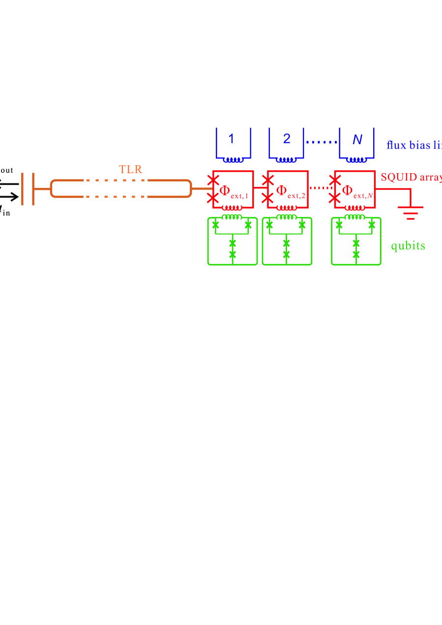
Figure A1: Schematics of a quarter-wavelength transmission-line resonator (TLR) terminated by an array of $N$ SQUIDs. The effective nonlinear inductance of the $j$th SQUID is controlled via the external flux $\Phi_{\text{ext},j}$, which contains a static part (produced by the $j$th bias line) and a perturbation part (produced by the circulating current of the $j$th flux qubit).

B.4 Multi-SQUID terminated resonator

As shown in Fig. A1, the one-dimensional transmission line resonator (TLR) can also be terminated in its right side by a series of $N$ dc SQUID Sandberg et al. (2008); Eichler and Wallraff (2014). Each SQUID can be tuned by via an independent external flux bias. The two Josephson junctions of the $j$th SQUID are symmetric with identical Josephson energy $E_{sj}$ and capacitance $C_{sj}$. The effective Josephson energy is tuned with the external flux $\Phi_{\text{ext},j}$ according to the relation $E_{j}=2E_{sj}\cos(\pi\Phi_{\text{ext},j}/\Phi_{0})$, and the nonlinear inductance is $L_{sj}(\Phi_{\text{ext},j})=\Phi_{0}^{2}/[(2\pi)^{2}E_{j}]$. The Lagrangian of the $j$th SQUID is

$$\mathcal{L}_{j}=\sum_{i=1,2}\left[\frac{\Phi_{0}^{2}}{2(2\pi)^{2}}C_{sj}(\dot{\phi_{ji}})^{2}-E_{sj}\cos{\phi_{ji}}\right],$$

where $\phi_{ji}$ is the phase difference of the $i$th junction in the $j$th SQUID. Similar to the single SQUID case, we obtain the boundary equation at the right-hand side of Eq. (B8) Sandberg et al. (2008):

$$\psi(d_{0},t)=\sum_{j}^{N}\phi_{j+}(t),$$ (B25a)

$$2C_{s}\ddot{\psi}(d_{0},t)+\frac{(2\pi)^{2}}{\Phi_{0}^{2}}E_{j}(\Phi_{\text{ext},j})\phi_{j+}(t)+\frac{\partial_{x}\psi(d_{0},t)}{L_{0}}=0,$$ (B25b)

where $\phi_{j+}=(\phi_{j1}+\phi_{j2})/2$. By expanding the left-hand side of Eq. (B25b) with $\omega_{r}/\omega_{0}$ around $\pi/2$ to first order, we obtain

$$\omega_{r}=\omega_{0}\left[1-\frac{\sum_{j}^{N}L_{sj}(\Phi_{\text{ext},j})}{L_{t}}\right],$$ (B26)

from which we can find that the external flux $\Phi_{\text{ext},j}$ through the $j$th SQUID determines its nonlinear inductance independently. Their joint effect eventually shifts the mode frequency to $\omega_{r}$. Similar to the discussions of the single-SQUID case, we obtain the resonator frequency $\omega_{r0}$ and the flux sensitivity $R_{j}$ of the $j$th SQUID as

$$\omega_{r0}=\omega_{0}\left[1-\sum_{j=1}^{N}\frac{L_{s}(\Phi_{\text{ext},j}^{0})}{L_{t}}\right],$$ (B27a)

$$R_{j}=\frac{\partial\omega_{r}}{\partial\Phi_{\text{ext},j}}\Big{|}_{\Phi_{\text{ext},j0}^{0}}=-\;\frac{\pi\omega_{0}L_{s}(\Phi_{\text{ext},j}^{0})}{\Phi_{0}L_{t}}\tan\!\left(\frac{\pi\Phi_{\text{ext},j}^{0}}{\Phi_{0}}\right).$$ (B27b)

Note that the above discussions can also be applied to the single-SQUID case by setting $N=1$. Assuming that the flux perturbations of the $j$th SQUID are produced by the circulating current of a single flux qubit as a quantum bus, then it is possible to dispersively couple multiple qubits with a single resonator. Employing this layout, we can achieve a multi-qubit QND readout.

Appendix C Circulating currents in the gradiometric flux qubit

As shown in Fig. A2(a), the gap-tunable flux qubit has a gradiometric topology by adopting an eight-shaped design, and the small $\alpha$-junction is replaced by a SQUID (the $\alpha$-loop). The gradiometric structure splits the persistent current symmetrically. This special geometric arrangement allows one to control the gap value $\alpha$ via the external flux $f_{\alpha}$ without disturbing the energy bias Paauw et al. (2009); Fedorov et al. (2010); Schwarz et al. (2013). We assume that the two junctions (with a gauge-invariant phase difference $\varphi_{1,2}$) in the main loop have the same Josephson energy $E_{J}$ and capacitance $C$. The other two junctions in the SQUID loop (with a gauge-invariant phase difference $\varphi_{3,4}$), are also identical but with smaller Josephson energies and capacitances by a factor $\alpha_{0}$ compared to the junctions in the main loop. Because the loop inductance is usually much smaller than the effective nonlinear junction, we neglect the phase accumulated along each loop circumference. Therefore, the fluxoid quantization conditions of the $f_{\alpha}$, $f_{\epsilon 1}$ and $f_{\epsilon 2}$ loop are Paauw (2009); Schwarz (2015):

$$\varphi_{3}-\varphi_{4}+2\pi f_{\alpha}=2\pi N_{\alpha},$$ (C1a)

$$\varphi_{3}+\varphi_{1}+\varphi_{2}+2\pi f_{\epsilon 1}=2\pi N_{\epsilon 1},$$ (C1b)

$$-\varphi_{4}-\varphi_{1}-\varphi_{2}+2\pi f_{\epsilon 2}=2\pi N_{\epsilon 2},$$ (C1c)

where $N_{\alpha}$ and $N_{\epsilon 1,\epsilon 2}$ are the integer numbers of the trapped fluxoids, and $f_{\alpha,\epsilon 1(2)}=\Phi_{\alpha,\epsilon 1(2)}/\Phi_{0}$ with $\Phi_{\alpha}$ ($\Phi_{\epsilon 1(2)}$) being the external flux through the $f_{\alpha}$ ($f_{\epsilon 1,2}$) loop. We assume $N_{\alpha}=0$. By setting $n=N_{\epsilon 2}-N_{\epsilon 1}$ and $f_{\epsilon}=\Phi_{\epsilon}/\Phi_{0}=f_{\epsilon 1}-f_{\epsilon 2}$, the above boundary conditions reduce the freedom of the systems and, thus, $\varphi_{3,4}$ can be given in terms of $\varphi_{1,2}$

$$\varphi_{3,4}=-\pi(n+f_{\epsilon})-(\varphi_{1}+\varphi_{2})\mp\pi f_{\alpha}.$$ (C2)

The Josephson energy (or the potential energy) for this four-junction system as a function of $\varphi_{1}$ and $\varphi_{2}$ is expressed as:

$$U/E_{J} = 2+2\alpha_{0}-\cos{\varphi_{1}}-\cos{\varphi_{2}}$$ (C3)

$$- 2\alpha_{0}\cos(\pi f_{\alpha})\cos{[\varphi_{1}+\varphi_{2}+\pi(n+f_{\epsilon})]}.$$

We now consider the charging energy stored in the capacitances of the four junctions in this circuit, and the kinetic energy has the form

$$T = \frac{1}{2}\left(\frac{\Phi_{0}}{2\pi}\right)^{2}\sum_{i=1}^{4}C_{i}\dot{\varphi}_{i}^{2}$$ (C4)

$$= \left(\frac{\Phi_{0}}{2\pi}\right)^{2}\!C\!\left[\frac{(1+2\alpha_{0})}{4}(\dot{\varphi}_{1}^{2}+\dot{\varphi}_{2}^{2})+\alpha_{0}\dot{\varphi}_{1}\dot{\varphi}_{2}\right],$$

where we have employed the relation $\dot{\varphi}_{3,4}=-(\dot{\varphi}_{1}+\dot{\varphi}_{2})$. The Lagrangian for the whole circuit is $\mathcal{L}=T-U$, from which we obtain the canonical momentum $p_{i}=\partial\mathcal{L}/(\partial\dot{\varphi}_{i})$ as the conjugate to the coordinate $\varphi_{i}$. Therefore, by employing a Legendre transformation, the corresponding Hamiltonian is written as

$$H = \sum_{i=1,2}p_{i}\dot{\varphi}_{i}-\mathcal{L}$$ (C5)

$$= \frac{4E_{c}}{1+4\alpha_{0}}[(1+2\alpha_{0})(p_{1}^{2}+p_{2}^{2})-4\alpha_{0}p_{1}p_{2})]$$

$$+E_{J}\big{\{}2+2\alpha_{0}-\cos{\varphi_{1}}-\cos{\varphi_{2}}$$

$$-2\alpha_{0}\cos(\pi f_{\alpha})\cos{[\varphi_{1}+\varphi_{2}+\pi(n+f_{\epsilon})]}\big{\}}.$$

To quantize the above Hamiltonian, we introduce the commutation relation $[\varphi_{i},p_{j}]=i\delta_{ij}$ with $p_{i}=-i\partial/\partial\varphi_{i}$.

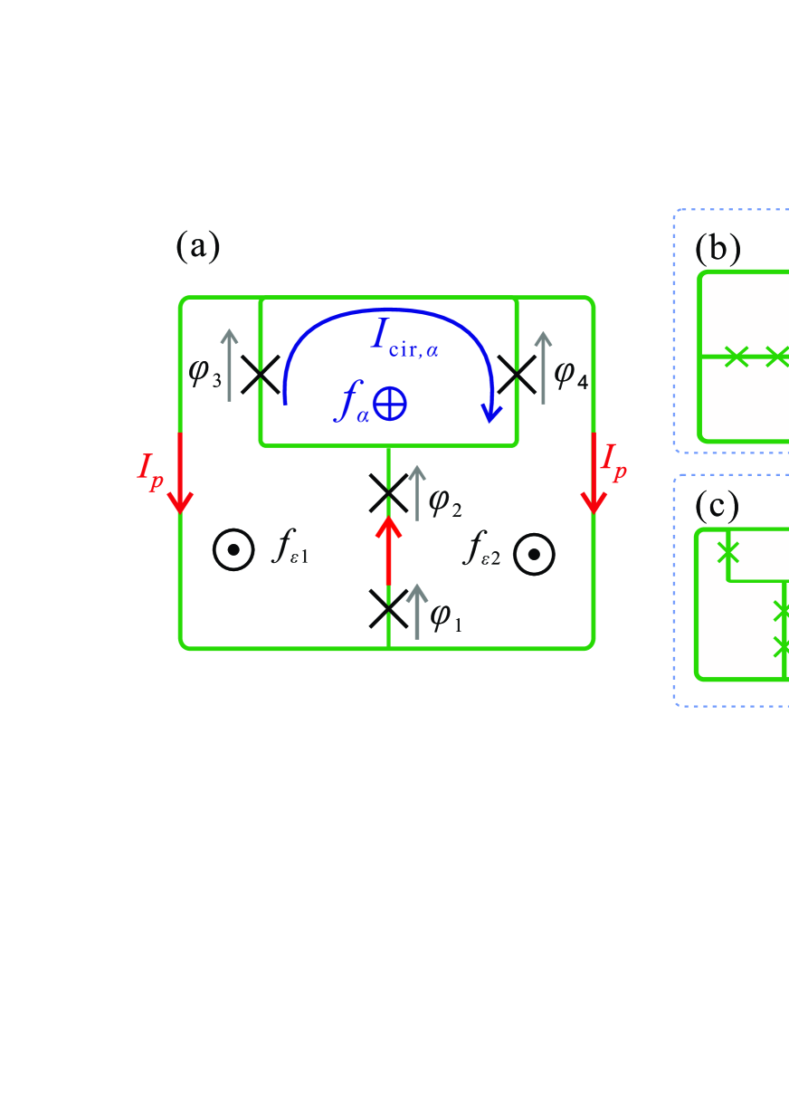
Figure A2: (a) Schematic diagram for a gradiometric flux qubit. The Josephson junctions are represented by the crosses. The phase difference across the $i$th junction is denoted by $\varphi_{i}$. The energy bias (energy gap) of the flux qubit is controlled via the reduced magnetic flux $f_{\epsilon 1(2)}=\Phi_{\epsilon 1(2)}/\Phi_{0}$ ($f_{\alpha}=\Phi_{\alpha}/\Phi_{0}$) through the two gradiometric loops ($\alpha$-loop). The persistent current $I_{p}$ (red arrows) is split into two symmetrical parts, which circulate around two identical gradiometric loops. Another quantized super-current $I_{\text{cir},\alpha}$ circulates in the $\alpha$-loop, which is usually employed to create the longitudinal coupling. (b,c) Schematics of a flux qubit interacting with a SQUID-terminated resonator via mutual inductance $M$ and circulating current $I$: (b) $M_{\alpha}$ and $I_{\text{cir},\alpha}$, (c) $M_{p}$ and $I_{p}$.

For a flux qubit, to minimize the dephasing induced by the flux noise in the main-loop, one usually operates the flux qubit at its degeneracy point with $f_{\epsilon}=0$. Moreover, under the condition $0<2\alpha_{0}\cos(\pi f_{\alpha})<1$, the potential $U$ has a double-well shape. The eigenproblem described by Eq. (C5) can be numerically solved in the plane-wave basis Orlando et al. (1999). As discussed in Ref. Paauw (2009), the two lowest energy-levels are well-separated from all the higher ones. The ground state $|g\rangle$ and the first excited state $|e\rangle$ are, respectively, symmetric and anti-symmetric along the axis $\varphi_{+}=\varphi_{1}+\varphi_{2}$, and can be approximately expressed as Schwarz (2015):

$$|g\rangle=\frac{1}{\sqrt{2}}(|+I_{p}\rangle+|-I_{p}\rangle),$$ (C6a)

$$|e\rangle=\frac{1}{\sqrt{2}}(|+I_{p}\rangle-|-I_{p}\rangle),$$ (C6b)

where $|\pm I_{p}\rangle$ are the two persistent-current states of the opposite directions in the main-loop Orlando et al. (1999); Mooij et al. (1999). To calculate the circulating current in the $\alpha$-loop, we focus our attention on the supercurrent through the junctions 3 and 4, which is expressed as

$$I_{3,4}=\frac{2\pi\alpha_{0}E_{J}}{\Phi_{0}}\sin(\varphi_{3,4})=I_{c}\sin(\varphi_{3,4}).$$ (C7)

Employing the relation in Eq. (C2) and expanding $I_{3,4}$ in the basis of $|g\rangle$ and $|e\rangle$, we obtain the current operator for the junctions 3 and 4 as follows

$$I_{3(4)}=\left(\begin{matrix}I_{3(4),ee}&I_{3(4),eg}\\ I_{3(4),ge}&I_{3(4),gg}\\ \end{matrix}\right)$$

$$\!=I_{c}\!\left(\begin{matrix}\langle e|\sin(\varphi_{+}\!\pm\!\pi f_{\alpha})|e\rangle&\langle e|\sin(\varphi_{+}\!\pm\!\pi f_{\alpha})|g\rangle\\ \langle g|\sin(\varphi_{+}\!\pm\!\pi f_{\alpha})|e\rangle&\langle g|\sin(\varphi_{+}\!\pm\!\pi f_{\alpha})|g\rangle\\ \end{matrix}\right)\!,$$ (C8)

Because $|g\rangle$ ($|e\rangle$) is of even (odd) parity with respect to $\varphi_{+}$ at the degeneracy point, it is easy to verify that

$$I_{3,ii}=-I_{4,ii}=\sin(\pi f_{\alpha})I_{c}\langle i|\cos(\varphi_{+})|i\rangle$$ (C9)

for $i=e,\,g$. Therefore, given that the qubit is in its excited (ground) state, the average current of the junctions 3 and 4 are of opposite signs, and they generate a circulating current with amplitude $I_{3,ee}$ ($I_{3,gg}$) in the $\alpha$-loop. For the off-diagonal terms, it can be easily verified that

$$I_{3,eg}=I_{4,eg}=\cos(\pi f_{\alpha})I_{c}\langle e|\sin(\varphi_{+})|g\rangle,$$ (C10)

which is, in fact, equal to the persistent-current $I_{p}$ of the main loop (related to the $\sigma_{x}$ operator). Therefore, the circulating current operator in the $\alpha$-loop and persistent current operator in the main-loop is expressed as

$$I_{\text{cir},\alpha}=\frac{I_{3}-I_{4}}{2}=I_{+}I_{0}+I_{-}\sigma_{z},$$ (C11a)

$$I_{p}^{\prime}=I_{3}+I_{4}=2I_{3,eg}\left(|e\rangle\langle g|+|g\rangle\langle e|\right)=I_{p}^{\prime}\sigma_{x},$$ (C11b)

where

$$I_{+}=(I_{3,ee}+I_{3,gg})/2,\quad I_{-}=(I_{3,ee}-I_{3,gg})/2,$$

and $I_{0}$ is the identity operator. The standard definition of the SQUID circulating current in Refs. Paauw (2009); Wang et al. (2011) also gives the same form for $I_{\text{cir},\alpha}$. From Eq. (C5) we find that the flux qubit is controlled by the external fluxes $f_{\alpha}$ and $f_{\epsilon}$. Assuming that $n=1$ and the flux qubit is prebiased at the optimal point $\{f_{\alpha},f_{\epsilon}\}=\{f_{\alpha 0},0\}$, the circulating currents $I_{p}^{\prime}$ and $I_{\text{cir},\alpha}$ can also be derived via a thermodynamic relation Orlando et al. (1999); Paauw (2009). Specifically, by considering the flux perturbations $\delta\!f_{\alpha}$ and $\delta\!f_{\epsilon}$, we can rewrite the Hamiltonian in Eq. (C5) as

$$H(f_{\alpha},f_{\epsilon})=H(f_{\alpha 0},f_{\epsilon 0})+\frac{\partial H}{\partial f_{\alpha}}\delta\!f_{\alpha}+\frac{\partial H}{\partial f_{\epsilon}}\delta\!f_{\epsilon}.$$ (C12)

In the basis of $|e\rangle$ and $|g\rangle$, it can be easily verified that the following thermodynamic relations hold Orlando et al. (1999); Paauw (2009)

$$\frac{\partial H}{\partial f_{\alpha}}=I_{\text{cir},\alpha}\Phi_{0};\qquad\frac{\partial H}{\partial f_{\epsilon}}=\frac{I_{p}^{\prime}}{2}\Phi_{0}.$$ (C13)

Therefore, we can rewrite Eq. (C12) as

$$H=\frac{1}{2}\omega_{q}\sigma_{z}+\frac{I_{p}^{\prime}}{2}\sigma_{x}\delta\Phi_{\epsilon}+(I_{+}I_{0}+I_{-}\sigma_{z})\delta\Phi_{\alpha}.$$ (C14)

where $\delta\Phi_{\alpha}=\delta\!f_{\alpha}\Phi_{0}$ and $\delta\Phi_{\epsilon}=\delta\!f_{\epsilon}\Phi_{0}$. The circulating currents $I_{\text{cir},\alpha}$ and $I^{\prime}_{p}$, obtained from the thermodynamic relation Eq. (C13) and the definitions in Eq. (C11b) lead to the same results. For the flux qubit working at its degeneracy point, the qubit transition frequency $\omega_{q}$ between $|e\rangle$ and $|g\rangle$ is determined by the control flux $f_{\alpha}$, and the dephasing resulting from the flux noise in $f_{\epsilon}$ vanishes to first-order. The effective persistent-current circulating in each symmetric main loop is divided by two due to the gradiometric topology, i.e., $I_{p}=I_{p}^{\prime}/2$.

In this gap-tunable flux qubit, the persistent current $I_{p}$ of the flux qubit is widely employed to create ($\sigma_{x}-$type) dipole couplings. The circulating current difference $I_{-}$ in the $\alpha$-loop, can be employed to induce longitudinal coupling ($\sigma_{z}-$type) Schwarz et al. (2013). As shown in Fig. A2(a) and A2(b), the circulating currents $I_{\text{cir},\alpha}$ and $I_{p}$ can produce a flux perturbation through the SQUID of the resonator via the mutual inductances $M_{\alpha}$ and $M_{p}$, respectively, which changes the effective length of the resonator. Specifically, in the basis of $|e\rangle$ and $|g\rangle$, the interaction between $I_{\text{cir},\alpha}$ and the SQUID-terminated resonator corresponds to NPDC.

Note that both circulating currents $I_{\text{cir},\alpha}$ and $I_{p}$ naturally enhance the qubit sensitivity to flux noises. The $1/f$-type flux noise of the $\alpha$-loop leads to the broadening of the qubit transition frequency $\omega_{q}$, which corresponds to a pure dephasing process ($T_{2}$). The flux noise through two gradiometric loops affects the qubit via the persistent-current operator $I_{p}\sigma_{x}$, which results in the energy-relaxation process ($T_{1}$). Similar to discussion in Ref. Martinis et al. (2003); Ithier et al. (2005); Koch et al. (2007), the relaxation and dephasing rates can be approximately written as

$$\Gamma_{1} = \frac{1}{T_{1}}\backsimeq\left(\frac{\partial H}{\partial f_{\epsilon}}\right)^{2}S_{\bot}(\omega_{q})=\left(I^{\prime}_{p}\Phi_{0}\right)^{2}S_{\bot}(\omega_{q}),$$

$$\Gamma_{f} = \frac{1}{T_{2}}\backsimeq\left(\frac{\partial H}{\partial f_{\alpha}}\right)A_{\alpha}=A_{\alpha}\left(I_{-}\Phi_{0}\right),$$ (C15)

where $S_{\bot}(\omega_{q})$ is the noise power at the qubit frequency, and $A_{\alpha}$ is the amplitude of the $1/f$-type flux noise in the $\alpha$-loop. Note that the nonzero current difference $I_{-}$ makes the qubit sensitive to the $1/f$ noise in the $\alpha$-loop. As in the following discussion, for the flux qubit, the amplitude of $I_{-}$ is usually lower than the persistent current $I_{p}$ by about one order of magnitude. Moreover, the experimental results reported in Ref. Fedorov et al. (2010) indicate that the flux noise $A_{\alpha}$ might be much smaller than that of the main loop. Therefore the dephasing rate induced by $I_{-}$ is possibly much slower than that in the case when the qubit is operating far away from its optimal point.

Appendix D Numerical results on coupling strength, nonlinearity, and decoherence

We now discuss a set of possible parameters for the SQUID-terminated nonlinear resonator. Our discussions are mainly based on the experimental parameters in Refs. Pogorzalek et al. (2017); Eichler and Petta (2018). We first consider a $\lambda/4$ resonator with fixed frequency $\omega_{0}\simeq 2\pi\times 6~{}\text{GHz}$ and total inductance $L_{t}=10~{}\text{nH}$. A rapid photon escape rate $\kappa$ enhances the speed of the qubit readout, and we set $\kappa/(2\pi)\simeq 16~{}\text{MHz}$ in the following discussion. By assuming $E_{s0}=2\pi\times 2.5~{}\text{THz}$, the flux sensitivity and the self-Kerr nonlinearity strength changing with the control flux have been shown in Fig. 2. The flux sensitivity is about $R/(2\pi)\simeq 16~{}\text{MHz}/(\text{m}\Phi_{0})$ with the Kerr nonlinearity $K_{D}/(2\pi)\simeq 110~{}\text{kHz}$ at $\Phi_{\text{ext}}\simeq 0.48\Phi_{0}$.

The flux (critical current) noise amplitude of the SQUID attached to the resonator can be set as $A_{1}=5\times 10^{-6}\Phi_{0}$ ($A_{2}=5\times 10^{-6}I_{c}$) Koch et al. (2007). Employing these parameters, the dephasing rates in Eq. (B24) are calculated as $\Gamma_{f,\Phi}/(2\pi)\simeq 75~{}\text{kHz}$ and $\Gamma_{f,I}/(2\pi)\simeq 30~{}\text{kHz}$. Therefore the reduction of $T_{2}$ due to these two dephasing processes can be neglected when compared with $\kappa$ in our discussions.

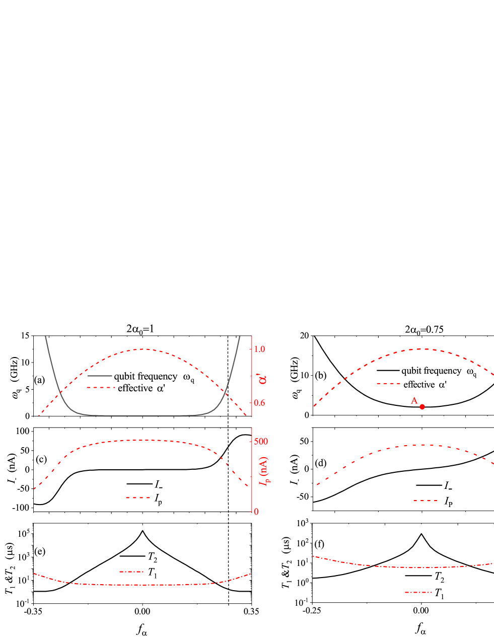
Figure A3: Flux-qubit parameters versus the external control flux $f_{\alpha}$ for $2\alpha_{0}=1$ (left panels) and $2\alpha_{0}=0.75$ (right panels). These parameters include: (a,b) the effective gap value $\alpha^{\prime}$, given in Eq. (D1), (red dashed curve) and the qubit frequency $\omega_{q}$ (black solid curve); (c,d) Circulating-current amplitudes $I_{-}$ (red dashed curve) and $I_{-}$ (black solid curve); and (e,f) the energy-relaxation times $T_{1}$ (red dash-dotted curve) and decoherence $T_{2}$ (black curve). In the left panels, the vertical line is at position $f_{\alpha}\simeq 0.27$. In (b), the points A and B correspond to $f_{\alpha}\simeq 0$ and $f_{\alpha}\simeq 0.22$, respectively. Here we assume $E_{J}/(2\pi)=320~{}\text{GHz}$ and $E_{J}/E_{C}=70$. The flux-noise amplitudes are set as $S_{\bot}(\omega_{q})=5\times 10^{-10}~{}\text{s}$ and $A_{\alpha}=5\times 10^{-6}$ according to Refs. Ithier et al. (2005); Koch et al. (2007).

To view the whole circuit in Fig. A2(a) as a flux qubit, the effective gap value

$$\alpha^{\prime}=2\alpha_{0}\cos(\pi f_{\alpha})$$ (D1)

should be in the range $0.5<\alpha^{\prime}<1$ Orlando et al. (1999), so that the double-well potential approximation is valid. In Fig. A3, we plot the qubit parameters changing with the external control flux $f_{\alpha}$ by setting $2\alpha_{0}=1$ (left panel) and $2\alpha_{0}=0.75$ (right panel), respectively. As shown in Fig. A3(a) and (b), the qubit frequency $\omega_{q}$ can be tuned in a wide range, when $f_{\alpha}$ is biased to be nonzero. The slope of $\omega_{q}$ changing with $f_{\alpha}$ is proportional to the circulating-current difference $I_{-}$ in the $\alpha$-loop [Eq. (C13)].

As shown in Fig. A3(a), the two-energy-level structure vanishes (i.e., $\omega_{q}=0$) at $f_{\alpha}=0$ for $2\alpha_{0}=1$. To obtain a qubit energy-level structure, we need to bias $f_{\alpha}$ far away from zero, for example, to the dashed-line position, where there is an effectively nonzero circulating current $I_{-}\simeq 60~{}\text{nA}$ [Fig. A3(c)]. When we keep on biasing $f_{\alpha}$, $I_{-}$ becomes larger. As described by Eq. (C15), increasing $I_{-}$ leads to a reduction of the pure dephasing time $T_{2}$. In Fig. A3(e), we find that the pure dephasing time $T_{2}$ decreases to about $1~{}\mu\text{s}$ at the dashed line position. In a gate operation, one may need a much longer qubit dephasing time. The experimental results in Ref. Fedorov et al. (2010) indicate that the flux noise in the $\alpha$-loop has a much lower amplitude than that in the main loop, and it is possible to obtain longer $T_{2}$ in experiments by reducing the $(1/f)$ noise amplitude $A_{\alpha}$.

Here we discuss another approach to increase $T_{2}$. In fact, by setting $2\alpha_{0}<1$, the qubit is insensitive to the first order of the flux noise in the $\alpha$-loop at $f_{\alpha}=0$, and the examples with $2\alpha_{0}=0.75$ are plotted in the right panel of Fig. A3. At $f_{\alpha}=0$ (point A), the qubit frequency is $\omega_{q}/(2\pi)\backsimeq 2~{}\text{GHz}$ with $I_{-}=0$. Because $I_{-}=0$, the qubit is insensitive, to first order of the $1/f$ flux noise, and $T_{2}$ is much longer than $1~{}\mu\text{s}$. When employing this qubit for quantum-information processing, one can operate it at the point A with much longer dephasing time. Once the qubit state is to be measured, the flux $f_{\alpha}$ is adiabatically biased away from zero without damping a given qubit state. As shown in Fig. A3(d), the circulating current $I_{\text{cir},\alpha}$ increases with $|f_{\alpha}|$. At $f_{\alpha}\backsimeq 0.22$ (Point B), $I_{\text{cir},\alpha}\backsimeq 50~{}\text{nA}$ and the dephasing time is about $T_{2}\sim 1~{}\mu\text{s}$. As discussed in Ref. Jeffrey et al. (2014), the qubit-readout time can be finished in tens of ns and therefore it is possible to perform several measurements within $T_{2}$. After finishing the measurements, one can adiabatically reset the flux bias $f_{\alpha}=0$ with a longer dephasing time for further quantum information processing. When considering the readout via changing the qubit frequency over such a large range, we should reconsider the parameters of the flux qubit carefully, e.g., the transition effects to higher-energy levels, and the degradation of the relaxation time $T_{1}$ and coherence time $T_{2}$. The breakdown of the adiabatic approximation, which indicates the coherence loss of the flux qubit, leads to a significantly lower readout fidelity.

As shown in Fig. A2(b), assuming that the qubit interacts with the resonator via mutual inductance $M_{\alpha}$, the circulating current $I_{\text{cir},\alpha}$ produces a small deviation part $\delta\Phi_{\text{ext}}=M_{\alpha}I_{\text{cir},\alpha}$, which can be detected by the resonator with a flux sensitivity $R$. Thus, the flux qubit can be coupled to the SQUID-terminated resonator. To enhance their coupling strength, we should employ a large mutual inductance to sense the circulating current. Assuming the mutual inductance between the $\alpha$-loop and the SQUID of the resonator is $M_{\alpha}$, the Hamiltonian for the whole system can be written as

$$H_{D} = \frac{\omega}{2}\sigma_{z}+\omega_{r0}a^{{\dagger}}a$$ (D2)

$$+ RM_{\alpha}(I_{+}I_{0}+I_{-}\sigma_{z})a^{{\dagger}}a+K_{D}a^{{\dagger}}a^{{\dagger}}aa$$

$$= \frac{\omega}{2}\sigma_{z}+\omega_{r}^{\prime}a^{{\dagger}}a+\chi_{z}^{D}\sigma_{z}a^{{\dagger}}a+K_{D}a^{{\dagger}}a^{{\dagger}}aa,$$

where $\chi_{z}^{D}=RM_{\alpha}I_{-}$ is the NPDC strength, and $\omega_{r}^{{}^{\prime}}=\omega_{r0}+RM_{\alpha}I_{+}$ is the renormalized mode frequency. One can find that this coupling has no relation to the dipole-field interactions. This qubit readout based on the Hamiltonian (D2) can be denoted as ideal QND measurement because $H_{D}$ commutes with the qubit operator $\sigma_{z}$.

As depicted in Fig. A3, we set $I_{\text{cir},\alpha}\backsimeq 60~{}\text{nA}$ and $I_{p}\backsimeq 300~{}\text{nA}$ in our discussion. To obtain strong coupling strengths, we can employ the kinetic inductance by sharing a qubit loop branch with the resonator SQUID. The kinetic mutual inductance is about $1\sim 3~{}\text{pH}/\mu\text{m}$, and can still be enhanced by reducing the wires cross-section area Meservey and Tedrow (1969); Paauw (2009); Schwarz (2015). The mutual inductance is about $15~{}\text{pH}$ with a shared loop length $\sim 5~{}\mu\text{m}$. Employing these parameters, we find that the coupling strengths are $\chi_{z}^{D}\backsimeq 7~{}\text{MHz}$ and $\chi_{x}^{D}\backsimeq 35~{}\text{MHz}$, respectively.

In the readout experiment with the IDC in Ref. Jeffrey et al. (2014), the Jaynes-Cummings coupling strength is about $g_{x}/(2\pi)=90~{}\text{MHz}$ with detuning $\Delta_{d}\simeq 1~{}\text{GHz}$, and the calculated IDC strength is about $\chi_{z}^{I}/(2\pi)\simeq 8~{}\text{MHz}$ with the qubit-state dependent Kerr nonlinearity $K_{I}/(2\pi)\simeq 65~{}\text{kHz}$. We find that it is reasonable to assume that $\chi_{z}^{I}=\chi_{z}^{D}$ and $K_{D}\simeq K_{I}$ in our discussions.

Moreover, we have plotted the energy relaxation time $T_{1}$ changing with $f_{\alpha}$. It can be found that $T_{1}$ varies over a much smaller scale that $T_{2}$. By assuming the noise power spectrum at the qubit frequency $S_{\bot}(\omega_{q})=(5\times 10^{-10})^{2}~{}\text{s}$ Ithier et al. (2005), the relaxation time is around $\Gamma_{1}^{-1}\backsimeq 9~{}\mu\text{s}$, which is of the same order as the experimental results Stern et al. (2014). In a qubit readout proposal based on IDC, the resonator usually has a quick decay rate. By setting the photon escaping rate $\kappa/(2\pi)=16~{}\text{MHz}$ and $\lambda=0.1$, the energy relaxation time due to the Purcell effect $T_{p}=\Gamma_{p}^{-1}$ is approximately $1~{}\mu\text{s}$. Because $\Gamma_{p}\gg\Gamma_{1}$, and it is reasonable to assume that the qubit decay is mainly limited by Purcell effects.

Appendix E Dispersive qubit readout without Purcell decay

From the discussions above, we find that the Kerr nonlinearity is involved in a qubit readout for both the IDC and NPDC readouts. However, these two nonlinearities are due to two different mechanisms: $K_{D}$ is due to attaching a nonlinear SQUID in the measurement resonator, while $K_{I}$ results from qubit dressing effects via the dipole-field coupling.

As shown in Fig. 1, at $t=0$ we apply an incident field $a_{\text{in}}$ in the left port at the shifted frequency of the resonator. In the interaction picture, the Langevin equations of the resonator operator, governed by Eq. (A4) (the IDC readout) and Eq. (D2) (the NPDC readout) can, respectively, be written as

$$\frac{da(t)}{dt} = -i\chi_{z}^{I}\sigma_{z}a(t)-2iK_{I}\langle n(t)\rangle\sigma_{z}a(t)$$ (E1)

$$- \frac{1}{2}\kappa a(t)-\sqrt{\kappa}a_{\text{in}}(t),$$

$$\frac{da(t)}{dt} = -i\chi_{z}^{D}\sigma_{z}a(t)-2iK_{D}\langle n(t)\rangle a(t)$$ (E2)

$$- \frac{1}{2}\kappa a(t)-\sqrt{\kappa}a_{\text{in}}(t),$$

where $\langle n(t)\rangle=\langle a^{{\dagger}}(t)a(t)\rangle$ is the time-dependent photon number in the resonator. The Kerr term $K_{I}$ in Eq. (E1) is dependent on the qubit state, i.e., is related to the Pauli operator $\sigma_{z}$; while the Kerr nonlinearity $K_{D}$ in Eq. (E2) is a standard Kerr term. This input field $a_{\text{in}}(t)=\alpha_{\text{in}}-d_{\text{in}}(t)$ is assumed to be characterized by its mean value (a coherent drive) $\alpha_{\text{in}}=-\epsilon\exp(i\theta_{d})/\sqrt{\kappa}$ and a fluctuation part $d_{\text{in}}(t)$. To compare the qubit readout process for these two different mechanisms, we assume $\chi_{z}^{I}=\chi_{z}^{D}=\chi_{z}$ and $K_{D}=K_{I}=K$ in the following discussion.

Below we start from the ideal readout without the Kerr nonlinearity, i.e., $K=0$, and give an analytical form for the measurement fidelity. After that, we reconsider the nonlinear effects in these two cases.

E.1 Ideal readout: Measurement without Kerr nonlinearity

By setting $K_{D}=K_{I}=K=0$, we obtain the same linear Langevin differential equation from both Eqs. (E1) and (E2). The average part of the output field is obtained from the input-output boundary condition

$$\alpha_{\text{out}}=\sqrt{\kappa}\alpha_{r}(t)-\epsilon\exp(i\theta_{d})/\sqrt{\kappa},$$

where $\alpha_{r}(t)$ is the average field of the resonator, and is derived by formally integrating the Langevin differential equation Didier et al. (2015b):

$$\alpha_{r}(t) = \frac{\epsilon\sqrt{\kappa}\exp\left[i(\theta_{d}-\langle\sigma_{z}\rangle\theta_{q})\right]}{\sqrt{\frac{1}{4}\kappa^{2}+(\chi_{z}\langle\sigma_{z}\rangle)^{2}}}$$ (E3)

$$\times\left\{1-\exp\left[-(i\chi_{z}\langle\sigma_{z}\rangle+\frac{1}{2}\kappa)t\right]\right\},$$

where $\theta_{q}=\arctan({2\chi_{z}/\kappa})$ is the rotating angle of the output field due to the dispersive coupling. The average intracavity photon number is written as in Eq. (11). The output fluctuation part $d_{\text{out}}(\omega)$ in Fourier space can also be obtained from the Langevin differential equation, and is expressed as

$$d_{\text{out}}(\omega)=\left[1-\frac{\kappa}{i(\omega+\chi_{z}\langle\sigma_{z}\rangle)+\frac{1}{2}\kappa}\right]d_{\text{in}}(\omega)$$ (E4)

One find that Eq. (E4) leads to completely different expressions for different types of input noise $d_{\text{in}}(\omega)$, (e.g., the vacuum, single-, and multi-mode squeezed vacuum). For simplicity, we assume that $d_{\text{in}}(t)$ is the vacuum without squeezing, and satisfies the correlation relation $\langle d_{\text{in}}(\omega)d_{\text{in}}^{{\dagger}}(\omega^{\prime})\rangle=\delta(\omega+\omega^{\prime})$.

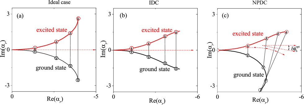
Figure A4: Evolutions in the phase space of the intracavity field for (a) the ideal [(Eq. E3)], (b) IDC [(Eq. E1)], and (c) NPDC [(Eq. E2)] readouts. The red (black) curves correspond to the qubit being in its excited (ground) state, and the black solid arrows connecting two circles represent the separations between two signals at the same time $t$. In (c), $\delta\phi_{h}^{\text{opt}}$ indicates the rotated optimal homodyne angle for a homodyne measurement. In these plots, both Kerr nonlinearity and Purcell effects are considered. The parameters used here are the same as those in Fig. 4(d), and the drive strength is assumed to be the same as for the stop point.

Due to the dispersive coupling, the qubit in its ground or excited states corresponds to rotating the output field in phase space with two different angles. The qubit state is encoded in the output quadrature $Y(\phi_{h})=a_{\text{out}}^{{\dagger}}e^{i\phi_{h}}+a_{\text{out}}e^{-i\phi_{h}}$ with $\phi_{h}$ being the homodyne-measurement angle. The output signal corresponds to a standard homodyne detection of the quadrature $Y(\phi_{h})$, with an integration time $\tau$, and has the following form

$$M(\tau)=\sqrt{\kappa}\int_{0}^{\tau}dt\left[a_{\text{out}}^{{\dagger}}(t)\exp(i\phi_{h})+a_{\text{out}}(t)\exp(-i\phi_{h})\right],$$ (E5)

By setting $\langle\sigma_{z}\rangle=\pm 1$ in Eq. (E3), respectively, one obtains the expression for the separation signal given in Eq. (10). On the other hand, the fluctuations $d_{\text{out}}(t)$ brings noise into the measurement signal. The integrated imprecision noise $M_{N}(\tau)$ is identical for the qubit ground and excited states, and is expressed as Didier et al. (2015b)

$$M_{N}^{2}(\tau) = [\langle M_{N}^{2}(\tau)\rangle_{|e\rangle}+\langle M_{N}^{2}(\tau)\rangle_{|g\rangle}]$$ (E6)

$$= 2\kappa\left\{\int_{0}^{\tau}\!\!dt[d_{\text{out}}^{{\dagger}}(t)e^{i\phi_{h}}\!+\text{H.c.}]\right\}^{2}\!=\!2\kappa\tau.$$

According to Eq. (10), the signal $M_{s}(\tau)$ is optimized by setting $\phi_{h}^{\prime}=\theta_{d}-\phi_{h}=\pi/2$ and $\theta_{q}=\pi/4$ (i.e., $\chi_{z}=\kappa/2$) in the long-time limit with $\kappa\tau\gg 1$. In Fig. A4(a), by adopting the same parameters as those in Fig. 3(d) in the main article (the drive strength is assumed at the stop point), we plot the evolution of the intracavity fields in phase space. The red and black curves represent the qubit in its excited and ground states, respectively. The two circles connected by the same black arrow correspond to the same time $t$. We find that the separation direction between these two signals in phase space is along the black solid arrows and is always vertical to the red dashed arrow, which corresponds to the optimal relative angle $\phi_{h}^{\prime}=\theta_{d}-\phi_{h}=\pi/2$ of a homodyne measurement. The signal-to-noise-ratio (SNR) becomes

$$\mathcal{R} = \frac{M_{s}(\tau)}{M_{N}(\tau)}$$ (E7)

$$= \frac{2\epsilon\sqrt{2\kappa\tau}}{\kappa}\!\left[\!1\!-\!\frac{2}{\kappa\tau}\left(1-e^{-\frac{1}{2}\kappa\tau}\cos\frac{1}{2}\kappa\tau\right)\right].$$

In the following discussion, we discuss the IDC and NPDC readouts. We find that the optimal measurement signal described in Eq. (E7) can be destroyed by both the Kerr and Purcell effects.

E.2 Kerr nonlinearity for the IDC- and NPDC-based readout mechanisms

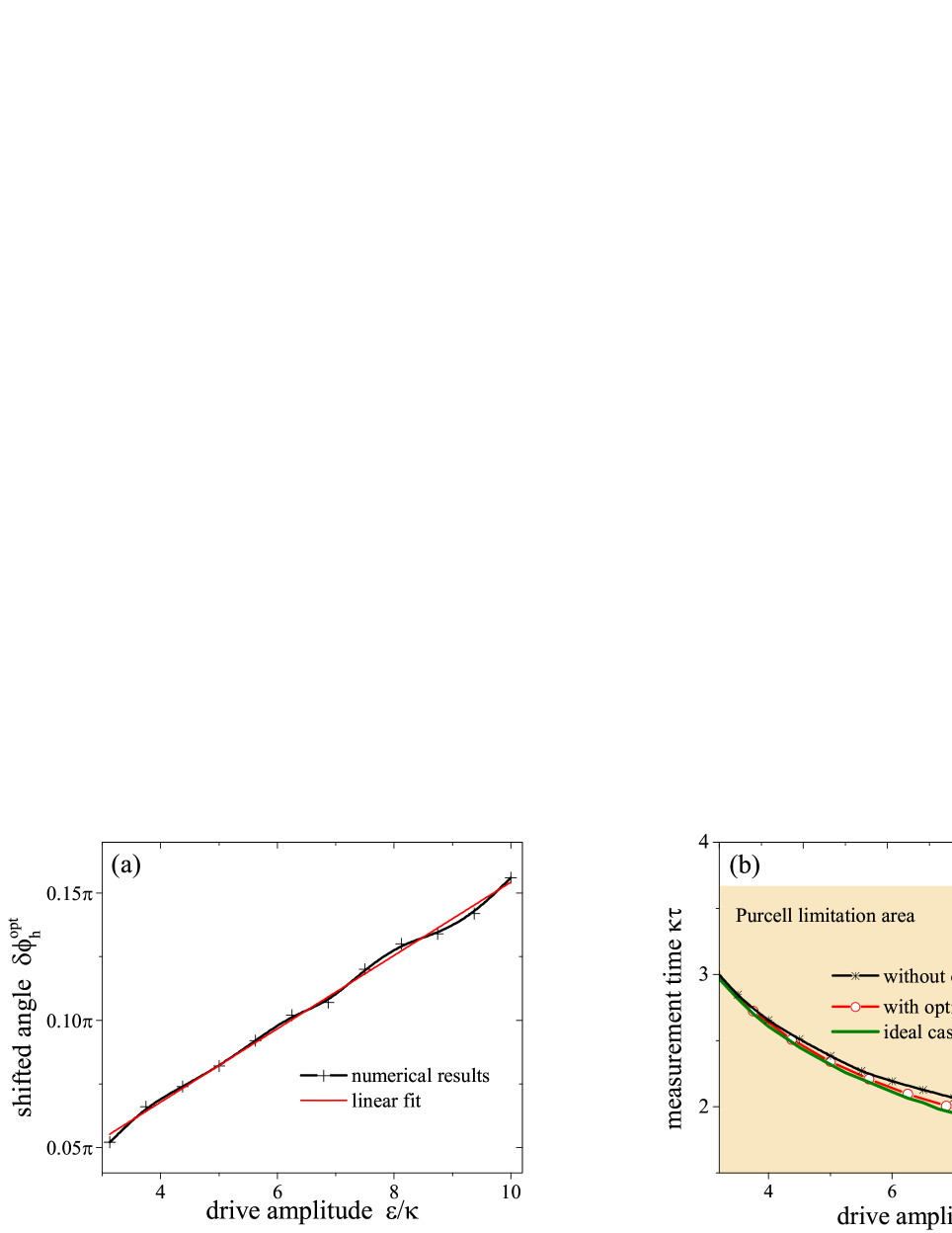
Figure A5: (a) Optimal shifted homodyne angle $\delta\phi_{h}^{\text{opt}}$ (corresponding to the shortest measurement time to reach $F=99.99\%$) versus the drive strength $\epsilon$ (in units of $\kappa$). The curve with crosses shows the numerical results, and the red curves show our linear fit according to the relation $\epsilon/\kappa=a\delta\phi_{h}^{\text{opt}}+b$. Here we set $a\simeq 0.144$ and $b\simeq 0.01$. (b) Required measurement time to reach the fidelity $F=99.99\%$ for the ideal readout [Eq. (E7)], the NPDC readouts with and without the shifted optimal angle $\delta\phi_{h}^{\text{opt}}$. The cyan area corresponds to the Purcell limitation area. The parameters here are the same as those in Fig. 4.

In the IDC readout, according to the nonlinear Langevin equation (E1), the effective cavity frequency pull $\xi_{g}(t)$ is reduced by the photon number due to the qubit-dependent Kerr terms, which can be written as:

$$\xi_{g}(t) = -\chi_{z}-2Kn_{g}(t)=-\chi_{z}\left[1-\frac{\langle n_{g}(t)\rangle}{2n_{c}}\right],$$ (E8)

$$\xi_{e}(t) = \chi_{z}+2Kn_{e}(t)=\chi_{z}\left[1-\frac{\langle n_{e}(t)\rangle}{2n_{c}}\right],$$ (E9)

where $\langle n_{g,e}(t)\rangle=\langle a^{\dagger}(t)a(t)\rangle\Big{|}_{g,e}$ is the mean photon number when the qubit is in its ground and excited states, respectively. As discussed in Ref. Boissonneault et al. (2009), Eq. (E9) indicates that with increasing the measuring photon number, the effective cavity pull $\xi$ is decreased. Specifically, when the intracavity number reaches $\langle n_{g,e}(t)\rangle=n_{c}$, the cavity pull is reduced as $\xi_{g,e}(t)=\chi_{z}/2$.

Because the qubit-dependent Kerr nonlinearity is symmetric for the ground and excited states, it can be easily verified that $\langle n_{g}(t)\rangle\simeq\langle n_{e}(t)\rangle$ and $\xi_{g}(t)\simeq-\xi_{e}(t)$. The reduction of the cavity pull $\xi_{g,e}(t)$ reduces the signal separation in phase space, which can be clearly found by comparing the numerical results in Figs. A4(b) and A4(a). With increasing time $t$, the separation distances (the black arrows) are significantly reduced compared with those in the ideal readout. Consequently, the required measurement time becomes longer. Therefore, for the IDC readout, increasing the intracavity photon number does not only enhance the qubit-error-transition probability (Purcell photon number limitations), but also reduces the measurement fidelity due to the Kerr nonlinearity $K$.

For the NPDC readout without the dipole-field coupling, because the intracavity photons do not deteriorate the qubit states, there is no qubit-error-transition due to the Purcell effects. However, when $\langle n(t)\rangle$ is large, the Kerr nonlinearity (introduced by the SQUID) induces apparent effects. Different from the IDC readout, the nonlinearity is not qubit-dependent, and the changing of the cavity pull for the two qubit states is not symmetric. For $K<0$, the cavity pulls for the qubit being in its ground and excited state are, respectively,

$$\xi_{g}(t)=-\chi_{z}+2Kn_{g}(t),\quad\xi_{e}(t)=\chi_{z}+2Kn_{e}(t),$$ (E10)

from which we can find that, by increasing the photon number, the effective cavity pull $|\xi_{g}|$ ($|\xi_{e}|$) increases (decreases). This leads to asymmetric rotation angles of the cavity field for the qubit in the ground and excited states, which can be clearly found from Fig. A4(c). The evolutions for the ground and excited states in phase space are asymmetric. The signal separation direction (black arrows) is now time-dependent and rotates in phase space. However, the signal separation distance is still large compared with the NPDC readout, and almost equal to that in the ideal readout.

In a homodyne experiment, one can tune the measurement angle $\phi_{h}^{\prime}$ for the NPDC readout, to maximize the total signal separation $M_{s}(\tau)$ during the integrating time $\tau$. As sketched in Fig. A4(c), $\phi_{h}^{\prime}$ can only be slightly shifted with an amount $\delta\phi_{h}^{\prime}$. For a certain drive strength $\epsilon$, there exists an optimal shifted angle $\delta\phi_{h}^{\text{opt}}$, which corresponds to the shortest measurement time for a certain fidelity. In Fig. A5(a), by adopting the same parameters as those in Fig. 3 of the main article (with $F=99.99\%$), we plot $\delta\phi_{h}^{\text{opt}}$ changing with $\epsilon$. It can be found that, with a stronger drive strength $\epsilon$, we need a larger optimal shifted angle $\delta\phi_{h}^{\text{opt}}$. Their relation can be approximately described by a simple linear function $\epsilon/\kappa=a\delta\phi_{h}^{\text{opt}}+b$ (red curve). In Fig. A5(b), we plot the required measurement time to reach the fidelity $F=99.99\%$ for the ideal readout, the NPDC readout with and without shifted optimal angle $\delta\phi_{h}^{\text{opt}}$. We find that, even without shifted optimal angle (curve with asterisks), the measurement can still go into the Purcell limitation area of the IDC readout (yellow area, below the stop point in Fig. 4). If we choose the optimal shifted angle $\delta\phi_{h}^{\text{opt}}$, the required time can still be shortened (curve with circles), and it is close to that of the ideal readout (green solid curve). Therefore, by slightly rotating the measurement angle, the measurement time can go far below the Purcell limitation area compared with the IDC readout.

References

- DiVincenzo (2009) D. P. DiVincenzo, “Fault-tolerant architectures for superconducting qubits,” Phys. Scr. T137, 014020 (2009).
- Ashhab et al. (2009) S. Ashhab, J. Q. You, and F. Nori, “Weak and strong measurement of a qubit using a switching-based detector,” Phys. Rev. A 79, 032317 (2009).
- Kelly et al. (2015) J. Kelly, R. Barends, A. G. Fowler, A. Megrant, E. Jeffrey, T. C. White, D. Sank, J. Y. Mutus, B. Campbell, Y. Chen, Z. Chen, B. Chiaro, A. Dunsworth, I.-C. Hoi, C. Neill, P. J. J. O’Malley, C. Quintana, P. Roushan, A. Vainsencher, J. Wenner, A. N. Cleland, and J. M. Martinis, “State preservation by repetitive error detection in a superconducting quantum circuit,” Nature (London) 519, 66–69 (2015).
- Terhal (2015) B. M. Terhal, “Quantum error correction for quantum memories,” Rev. Mod. Phys. 87, 307–346 (2015).
- Raussendorf and Harrington (2007) R. Raussendorf and J. Harrington, “Fault-tolerant quantum computation with high threshold in two dimensions,” Phys. Rev. Lett. 98, 190504 (2007).
- Barends et al. (2014) R. Barends, J. Kelly, A. Megrant, A. Veitia, D. Sank, E. Jeffrey, T. C. White, J. Mutus, A. G. Fowler, B. Campbell, Y. Chen, Z. Chen, B. Chiaro, A. Dunsworth, C. Neill, P. O’Malley, P. Roushan, A. Vainsencher, J. Wenner, A. N. Korotkov, A. N. Cleland, and J. M. Martinis, “Superconducting quantum circuits at the surface code threshold for fault tolerance,” Nature (London) 508, 500–503 (2014).
- Fowler et al. (2012) A. G. Fowler, M. Mariantoni, J. M. Martinis, and A. N. Cleland, “Surface codes: Towards practical large-scale quantum computation,” Phys. Rev. A 86, 032324 (2012).
- You and Nori (2003) J. Q. You and F. Nori, “Quantum information processing with superconducting qubits in a microwave field,” Phys. Rev. B 68, 064509 (2003).
- Gu et al. (2017) X. Gu, A. F. Kockum, A. Miranowicz, Y.-X. Liu, and F. Nori, “Microwave photonics with superconducting quantum circuits,” Phys. Rep. 718-719, 1–102 (2017).
- Blais et al. (2004) A. Blais, R.-S. Huang, A. Wallraff, S. M. Girvin, and R. J. Schoelkopf, “Cavity quantum electrodynamics for superconducting electrical circuits: An architecture for quantum computation,” Phys. Rev. A 69, 062320 (2004).
- Mallet et al. (2009) F. Mallet, F. R. Ong, A. Palacios-Laloy, F. Nguyen, P. Bertet, D. Vion, and D. Esteve, “Single-shot qubit readout in circuit quantum electrodynamics,” Nat. Phys. 5, 791 (2009).
- Kockum et al. (2012) A. F. Kockum, L. Tornberg, and G. Johansson, “Undoing measurement-induced dephasing in circuit QED,” Phys. Rev. A 85, 052318 (2012).
- Gustavsson et al. (2013) S. Gustavsson, O. Zwier, J. Bylander, F. Yan, F. Yoshihara, Y. Nakamura, T. P. Orlando, and W. D. Oliver, “Improving quantum gate fidelities by using a qubit to measure microwave pulse distortions,” Phys. Rev. Lett. 110, 040502 (2013).
- Diniz et al. (2013) I. Diniz, E. Dumur, O. Buisson, and A. Auffèves, “Ultrafast quantum nondemolition measurements based on a diamond-shaped artificial atom,” Phys. Rev. A 87, 033837 (2013).
- Wallraff et al. (2005) A. Wallraff, D. I. Schuster, A. Blais, L. Frunzio, J. Majer, M. H. Devoret, S. M. Girvin, and R. J. Schoelkopf, “Approaching unit visibility for control of a superconducting qubit with dispersive readout,” Phys. Rev. Lett. 95, 060501 (2005).
- Bultink et al. (2018) C. C. Bultink, B. Tarasinski, N. Haandbæk, S. Poletto, N. Haider, D. J. Michalak, A. Bruno, and L. DiCarlo, “General method for extracting the quantum efficiency of dispersive qubit readout in circuit QED,” Appl. Phys. Lett. 112, 092601 (2018).
- Didier et al. (2015a) N. Didier, A。 Kamal, W。 D. Oliver, A。 Blais, and A。 A. Clerk, “Heisenberg-limited qubit read-out with two-mode squeezed light,” Phys. Rev. Lett. 115, 093604 (2015a).
- Wu et al. (2018) Y. L. Wu, L. P. Yang, M. Gong, Y. R. Zheng, H. Deng, Z. G. Yan, Y. J. Zhao, K. Q. Huang, A. D. Castellano, W. J. Munro, K. Nemoto, D. N. Zheng, C. P. Sun, Y. X. Liu, X. B. Zhu, and L. Lu, “An efficient and compact switch for quantum circuits,” Npj Quantum Information 4, 50 (2018).
- Rosenberg et al. (2017) D. Rosenberg, D. Kim, R. Das, D. Yost, S. Gustavsson, D. Hover, P. Krantz, A. Melville, L. Racz, G. O. Samach, S. J. Weber, F. Yan, J. L. Yoder, A. J. Kerman, and W. D. Oliver, “3D integrated superconducting qubits,” Npj Quantum Information 3, 42 (2017).
- Yan et al. (2018) F. Yan, P. Krantz, Y. Sung, M. Kjaergaard, D. L. Campbell, T. P. Orlando, S. Gustavsson, and W. D. Oliver, “Tunable coupling scheme for implementing high-fidelity two-qubit gates,” Phys. Rev. Applied 10, 054062 (2018).
- Goetz et al. (2018) J. Goetz, F. Deppe, K. G. Fedorov, P. Eder, M. Fischer, S. Pogorzalek, E. Xie, A. Marx, and R. Gross, “Parity-engineered light-matter interaction,” Phys. Rev. Lett. 121, 060503 (2018).
- Orgiazzi et al. (2016) J.-L. Orgiazzi, C. Deng, D. Layden, R. Marchildon, F. Kitapli, F. Shen, M. Bal, F. R. Ong, and A. Lupascu, “Flux qubits in a planar circuit quantum electrodynamics architecture: Quantum control and decoherence,” Phys. Rev. B 93, 104518 (2016).
- Peltonen et al. (2018) J. T. Peltonen, P. C. J. J. Coumou, Z. H. Peng, T. M. Klapwijk, J. S. Tsai, and O. V. Astafiev, “Hybrid rf SQUID qubit based on high kinetic inductance,” Sci. Rep. 8 (2018), 10.1038/s41598-018-27154-1.
- Armata et al. (2017) F. Armata, G. Calajo, T. Jaako, M. S. Kim, and P. Rabl, “Harvesting multiqubit entanglement from ultrastrong interactions in circuit quantum electrodynamics,” Phys. Rev. Lett. 119, 183602 (2017).
- Boissonneault et al. (2008) M. Boissonneault, J. M. Gambetta, and A. Blais, “Nonlinear dispersive regime of cavity QED: The dressed dephasing model,” Phys. Rev. A 77, 060305 (2008).
- Zueco et al. (2009) D. Zueco, G. M. Reuther, S. Kohler, and P. Hänggi, “Qubit-oscillator dynamics in the dispersive regime: Analytical theory beyond the rotating-wave approximation,” Phys. Rev. A 80, 033846 (2009).
- Boissonneault et al. (2009) M. Boissonneault, J. M. Gambetta, and A. Blais, “Dispersive regime of circuit QED: Photon-dependent qubit dephasing and relaxation rates,” Phys. Rev. A 79, 013819 (2009).
- Didier et al. (2015b) N. Didier, J. Bourassa, and A. Blais, “Fast quantum nondemolition readout by parametric modulation of longitudinal qubit-oscillator interaction,” Phys. Rev. Lett. 115, 203601 (2015b).
- Houck et al. (2008) A. A. Houck, J. A. Schreier, B. R. Johnson, J. M. Chow, J. Koch, J. M. Gambetta, D. I. Schuster, L. Frunzio, M. H. Devoret, S. M. Girvin, and R. J. Schoelkopf, “Controlling the spontaneous emission of a superconducting transmon qubit,” Phys. Rev. Lett. 101, 080502 (2008).
- Jeffrey et al. (2014) E. Jeffrey, D. Sank, J. Y. Mutus, T. C. White, J. Kelly, R. Barends, Y. Chen, Z. Chen, B. Chiaro, A. Dunsworth, A. Megrant, P. J. J. O’Malley, C. Neill, P. Roushan, A. Vainsencher, J. Wenner, A. N. Cleland, and J. M. Martinis, “Fast accurate state measurement with superconducting qubits,” Phys. Rev. Lett. 112, 190504 (2014).
- De Liberato (2014) S. De Liberato, “Light-matter decoupling in the deep strong coupling regime: The breakdown of the Purcell effect,” Phys. Rev. Lett. 112, 016401 (2014).
- Govia and Clerk (2017) L. C. G. Govia and A. A. Clerk, “Enhanced qubit readout using locally generated squeezing and inbuilt Purcell-decay suppression,” New J. Phys. 19, 023044 (2017).
- B. T. Gard (2018) J. Aumentado R. W. Simmonds B. T. Gard, K. Jacobs, “Fast, high-fidelity, quantum non-demolition readout of a superconducting qubit using a transverse coupling,” arXiv:1809.02597 (2018).
- Sete et al. (2015) E. A. Sete, J. M. Martinis, and A. N. Korotkov, “Quantum theory of a bandpass Purcell filter for qubit readout,” Phys. Rev. A 92, 012325 (2015).
- Walter et al. (2017) T. Walter, P. Kurpiers, S. Gasparinetti, P. Magnard, A. Potočnik, Y. Salathé, M. Pechal, M. Mondal, M. Oppliger, C. Eichler, and A. Wallraff, “Rapid high-fidelity single-shot dispersive readout of superconducting qubits,” Phys. Rev. Applied 7, 054020 (2017).
- Fedorov et al. (2010) A. Fedorov, A. K. Feofanov, P. Macha, P. Forn-Díaz, C. J. P. M. Harmans, and J. E. Mooij, “Strong coupling of a quantum oscillator to a flux qubit at its symmetry point,” Phys. Rev. Lett. 105, 060503 (2010).
- You et al. (2008) J. Q. You, Y.-X. Liu, and F. Nori, “Simultaneous cooling of an artificial atom and its neighboring quantum system,” Phys. Rev. Lett. 100, 047001 (2008).
- Paauw et al. (2009) F. G. Paauw, A. Fedorov, C. J. P. M Harmans, and J. E. Mooij, “Tuning the gap of a superconducting flux qubit,” Phys. Rev. Lett. 102, 090501 (2009).
- Paauw (2009) F. G. Paauw, Superconducting flux qubits: Quantum chains and tunable qubits, Ph.D. Thesis, Technische Universiteit Delft, Delft (2009).
- Schwarz et al. (2013) M J Schwarz, J Goetz, Z Jiang, T Niemczyk, F Deppe, A Marx, and R Gross, “Gradiometric flux qubits with a tunable gap,” New J. Phys. 15, 045001 (2013).
- You et al. (2007a) J. Q. You, Y.-X. Liu, C. P. Sun, and F. Nori, “Persistent single-photon production by tunable on-chip micromaser with a superconducting quantum circuit,” Phys. Rev. B 75, 104516 (2007a).
- You et al. (2007b) J. Q You, X. Hu, S. Ashhab, and F. Nori, “Low-decoherence flux qubit,” Phys. Rev. B 75, 140515 (2007b).
- You and Nori (2011) J. Q. You and F. Nori, “Atomic physics and quantum optics using superconducting circuits,” Nature (London) 474, 589 (2011).
- Xiang et al. (2013) Z. L. Xiang, S. Ashhab, J. Q. You, and F. Nori, “Hybrid quantum circuits: Superconducting circuits interacting with other quantum systems,” Rev. Mod. Phys. 85, 623–653 (2013).
- Mooij et al. (1999) J. E. Mooij, T. P. Orlando, L. Levitov, L. Tian, C. H. van der Wal, and S. Lloyd, “Josephson persistent-current qubit,” Science 285, 1036 (1999).
- Orlando et al. (1999) T. P. Orlando, J. E. Mooij, L. Tian, C. H. van der Wal, L. S. Levitov, S. Lloyd, and J. J. Mazo, “Superconducting persistent-current qubit,” Phys. Rev. B 60, 15398 (1999).
- Wang et al. (2011) Y.-D. Wang, X. B. Zhu, and C. Bruder, “Ideal quantum nondemolition measurement of a flux qubit at variable bias,” Phys. Rev. B 83, 134504 (2011).
- Stassi and Nori (2018) R. Stassi and F. Nori, “Long-lasting quantum memories: Extending the coherence time of superconducting artificial atoms in the ultrastrong-coupling regime,” Phys. Rev. A 97, 033823 (2018).
- Schwarz (2015) M. J. Schwarz, Gradiometric tunable-gap flux qubits in a circuit QED architecture, Ph.D. Thesis, Technische Universität München, München (2015).
- Lambert et al. (2018) N. Lambert, M. Cirio, M. Delbecq, G. Allison, M. Marx, S. Tarucha, and F. Nori, “Amplified and tunable transverse and longitudinal spin-photon coupling in hybrid circuit-QED,” Phys. Rev. B 97, 125429 (2018).
- Johnson et al. (2011) J. E. Johnson, E. M. Hoskinson, C. Macklin, D. H. Slichter, I. Siddiqi, and J. Clarke, “Dispersive readout of a flux qubit at the single-photon level,” Phys. Rev. B 84, 220503 (2011).
- Kakuyanagi et al. (2013) K. Kakuyanagi, S. Kagei, R. Koibuchi, S. Saito, A. Lupaşcu, K. Semba, and H. Nakano, “Experimental analysis of the measurement strength dependence of superconducting qubit readout using a Josephson bifurcation readout method,” New J. Phys. 15, 043028 (2013).
- Nakano et al. (2009) H. Nakano, S. Saito, K. Semba, and H. Takayanagi, “Quantum time evolution in a qubit readout process with a Josephson bifurcation amplifier,” Phys. Rev. Lett. 102, 257003 (2009).
- Kakuyanagi et al. (2015) K. Kakuyanagi, T. Baba, Y. Matsuzaki, H. Nakano, S. Saito, and K. Semba, “Observation of quantum Zeno effect in a superconducting flux qubit,” New J. Phys. 17, 063035 (2015).
- Wallquist et al. (2006) M. Wallquist, V. S. Shumeiko, and G. Wendin, “Selective coupling of superconducting charge qubits mediated by a tunable stripline cavity,” Phys. Rev. B 74, 224506 (2006).
- Sandberg et al. (2008) M. Sandberg, C. M. Wilson, F. Persson, T. Bauch, G. Johansson, V. Shumeiko, T. Duty, and P. Delsing, “Tuning the field in a microwave resonator faster than the photon lifetime,” Appl. Phys. Lett. 92, 203501 (2008).
- Johansson et al. (2010) J. R. Johansson, G. Johansson, C. M. Wilson, and F. Nori, “Dynamical Casimir effect in superconducting microwave circuits,” Phys. Rev. A 82, 052509 (2010).
- Johansson et al. (2009) J. R. Johansson, G. Johansson, C. M. Wilson, and F. Nori, “Dynamical Casimir effect in a superconducting coplanar waveguide,” Phys. Rev. Lett. 103, 147003 (2009).
- Wilson et al. (2011) C. M. Wilson, G. Johansson, A. Pourkabirian, M. Simoen, J. R. Johansson, T. Duty, F. Nori, and P. Delsing, “Observation of the dynamical Casimir effect in a superconducting circuit,” Nature (London) 479, 376–379 (2011).
- Johansson et al. (2014) J. R. Johansson, G. Johansson, and F. Nori, “Optomechanical-like coupling between superconducting resonators,” Phys. Rev. A 90, 053833 (2014).
- Eichler and Wallraff (2014) C. Eichler and A. Wallraff, “Controlling the dynamic range of a josephson parametric amplifier,” EPJ Quantum Technology 1, 1 (2014).
- Pogorzalek et al. (2017) S. Pogorzalek, K. G. Fedorov, L. Zhong, J. Goetz, F. Wulschner, M. Fischer, P. Eder, E. Xie, K. Inomata, T. Yamamoto, Y. Nakamura, A. Marx, F. Deppe, and R. Gross, “Hysteretic flux response and nondegenerate gain of flux-driven Josephson parametric amplifiers,” Phys. Rev. Applied 8, 024012 (2017).
- Eichler and Petta (2018) C. Eichler and J. R. Petta, “Realizing a circuit analog of an optomechanical system with longitudinally coupled superconducting resonators,” Phys. Rev. Lett. 120, 227702 (2018).
- Bourassa et al. (2012) J. Bourassa, F. Beaudoin, J. M. Gambetta, and A. Blais, “Josephson-junction-embedded transmission-line resonators: From Kerr medium to in-line transmon,” Phys. Rev. A 86, 013814 (2012).
- Richer and DiVincenzo (2016) S. Richer and D. DiVincenzo, “Circuit design implementing longitudinal coupling: A scalable scheme for superconducting qubits,” Phys. Rev. B 93, 134501 (2016).
- Richer et al. (2017) S. Richer, N. Maleeva, S. T. Skacel, I. M. Pop, and D. DiVincenzo, “Inductively shunted transmon qubit with tunable transverse and longitudinal coupling,” Phys. Rev. B 96, 174520 (2017).
- Billangeon et al. (2015a) P.-M. Billangeon, J. S. Tsai, and Y. Nakamura, “Scalable architecture for quantum information processing with superconducting flux qubits based on purely longitudinal interactions,” Phys. Rev. B 92, 020509 (2015a).
- Billangeon et al. (2015b) P.-M. Billangeon, J. S. Tsai, and Y. Nakamura, “Circuit-QED-based scalable architectures for quantum information processing with superconducting qubits,” Phys. Rev. B 91, 094517 (2015b).
- Ikonen et al. (2019) J. Ikonen, J. Goetz, J. Ilves, A. Keränen, A. M. Gunyho, M. Partanen, K. Y. Tan, D. Hazra, L. Grönberg, V. Vesterinen, S. Simbierowicz, J. Hassel, and M. Möttönen, “Qubit measurement by multichannel driving,” Phys. Rev. Lett. 122, 080503 (2019).
- Touzard et al. (2019) S. Touzard, A. Kou, N. E. Frattini, V. V. Sivak, S. Puri, A. Grimm, L. Frunzio, S. Shankar, and M. H. Devoret, “Gated conditional displacement readout of superconducting qubits,” Phys. Rev. Lett. 122, 080502 (2019).
- Zhang et al. (2019) W.-Y. Zhang, K. Kalashnikov, W.-S. Lu, P. Kamenov, T. DiNapoli, and M.E. Gershenson, “Microresonators fabricated from high-kinetic-inductance aluminum films,” Phys. Rev. Applied 11, 011003 (2019).
- Grünhaupt et al. (2018) L. Grünhaupt, N. Maleeva, S. T. Skacel, M. Calvo, F. Levy-Bertrand, A. V. Ustinov, H. Rotzinger, A. Monfardini, G. Catelani, and I. M. Pop, “Loss mechanisms and quasiparticle dynamics in superconducting microwave resonators made of thin-film granular aluminum,” Phys. Rev. Lett. 121, 117001 (2018).
- Niepce et al. (2019) David Niepce, Jonathan Burnett, and Jonas Bylander, “High kinetic inductance nanowire superinductors,” Phys. Rev. Applied 11, 044014 (2019).
- Meservey and Tedrow (1969) R. Meservey and P. M. Tedrow, “Measurements of the kinetic inductance of superconducting linear structures,” J. Appl. Phys. 40, 2028–2034 (1969).
- Annunziata et al. (2010) A. J. Annunziata, D. F. Santavicca, L. Frunzio, G. Catelani, M. J. Rooks, A. Frydman, and D. E Prober, “Tunable superconducting nanoinductors,” Nanotechnology 21, 445202 (2010).
- Natarajan et al. (2012) C. M. Natarajan, M. G. Tanner, and R. H. Hadfield, “Superconducting nanowire single-photon detectors: physics and applications,” Supercond. Sci. Technol. 25, 063001 (2012).
- Doerner et al. (2018) S Doerner, A Kuzmin, K Graf, I Charaev, S Wuensch, and M Siegel, “Compact microwave kinetic inductance nanowire galvanometer for cryogenic detectors at 4.2 K,” J. Phys. Commun. 2, 025016 (2018).
- Majer et al. (2007) J. Majer, J. M. Chow, J. M. Gambetta, J. Koch, B. R. Johnson, J. A. Schreier, L. Frunzio, D. I. Schuster, A. A. Houck, A. Wallraff, A. Blais, M. H. Devoret, S. M. Girvin, and R. J. Schoelkopf, “Coupling superconducting qubits via a cavity bus,” Nature (London) 449, 443–447 (2007).
- Grajcar et al. (2006) M. Grajcar, A. Izmalkov, S. H. W. van der Ploeg, S. Linzen, T. Plecenik, Th. Wagner, U. Hübner, E. Il’ichev, H.-G. Meyer, A. Yu. Smirnov, Peter J. Love, Alec Maassen van den Brink, M. H. S. Amin, S. Uchaikin, and A. M. Zagoskin, “Four-qubit device with mixed couplings,” Phys. Rev. Lett. 96, 047006 (2006).
- Grajcar et al. (2005) M. Grajcar, A. Izmalkov, S. H. W. van der Ploeg, S. Linzen, E. Il’ichev, Th. Wagner, U. Hübner, H.-G. Meyer, Alec Maassen van den Brink, S. Uchaikin, and A. M. Zagoskin, “Direct Josephson coupling between superconducting flux qubits,” Phys. Rev. B 72, 020503 (2005).
- Johansson et al. (2012) J. R. Johansson, P. D. Nation, and F. Nori, “Qutip: An open-source Python framework for the dynamics of open quantum systems,” Comput. Phys. Commun. 183, 1760 (2012).
- Johansson et al. (2013) J. R. Johansson, P. D. Nation, and F. Nori, “Qutip 2: A Python framework for the dynamics of open quantum systems,” Comput. Phys. Commun. 184, 1234 (2013).
- Gambetta et al. (2007) J. Gambetta, W. A. Braff, A. Wallraff, S. M. Girvin, and R. J. Schoelkopf, “Protocols for optimal readout of qubits using a continuous quantum nondemolition measurement,” Phys. Rev. A 76, 012325 (2007).
- Heinsoo et al. (2018) J. Heinsoo, C. K. Andersen, A. R., S. Krinner, T. Walter, Y. Salathé, S. Gasparinetti, J.-C. Besse, A. Potočnik, A. Wallraff, and C. Eichler, “Rapid high-fidelity multiplexed readout of superconducting qubits,” Phys. Rev. Appl. 10, 034040 (2018).
- Groen et al. (2013) J. P. Groen, D. Ristè, L. Tornberg, J. Cramer, P. C. de Groot, T. Picot, G. Johansson, and L. DiCarlo, “Partial-measurement backaction and nonclassical weak values in a superconducting circuit,” Phys. Rev. Lett. 111, 090506 (2013).
- Tan et al. (2015) D. Tan, S. J. Weber, I. Siddiqi, K. Mølmer, and K. W. Murch, “Prediction and retrodiction for a continuously monitored superconducting qubit,” Phys. Rev. Lett. 114, 090403 (2015).
- Cirio et al. (2017) M. Cirio, K. Debnath, N. Lambert, and F. Nori, “Amplified optomechanical transduction of virtual radiation pressure,” Phys. Rev. Lett. 119, 053601 (2017).
- Kockum et al. (2018) A. F. Kockum, A. Miranowicz, S. De Liberato, S. Savasta, and F. Nori, “Ultrastrong coupling between light and matter,” Nat. Rev. Phys. 1, 19 (2018).
- Wang et al. (2018) X. Wang, A. Miranowicz, and F. Nori, “Ideal quantum nondemolition readout of a flux qubit without Purcell limitations,” arXiv:1811.09048 (2018).
- R. Dassonneville (2019) V. Milchakov L. Planat É. Dumur F. Foroughi J. Puertas S. Leger K. Bharadwaj J. Delaforce C. Naud W. Hasch-Guichard J. J. García-Ripoll N. Roch O. Buisson R. Dassonneville, T. Ramos, “Fast high fidelity quantum non-demolition qubit readout via a non-perturbative cross-kerr coupling,” arXiv:1905.00271 (2019).
- Martinis et al. (2003) J. M. Martinis, S. Nam, J. Aumentado, K. M. Lang, and C. Urbina, “Decoherence of a superconducting qubit due to bias noise,” Phys. Rev. B 67, 094510 (2003).
- Ithier et al. (2005) G. Ithier, E. Collin, P. Joyez, P. J. Meeson, D. Vion, D. Esteve, F. Chiarello, A. Shnirman, Y. Makhlin, J. Schriefl, and G. Schön, “Decoherence in a superconducting quantum bit circuit,” Phys. Rev. B 72, 134519 (2005).
- Deppe et al. (2007) F. Deppe, M. Mariantoni, E. P. Menzel, S. Saito, K. Kakuyanagi, H. Tanaka, T. Meno, K. Semba, H. Takayanagi, and R. Gross, “Phase coherent dynamics of a superconducting flux qubit with capacitive bias readout,” Phys. Rev. B 76, 214503 (2007).
- Koch et al. (2007) J. Koch, T. M. Yu, J. Gambetta, A. A. Houck, D. I. Schuster, J. Majer, A. Blais, M. H. Devoret, S. M. Girvin, and R. J. Schoelkopf, “Charge-insensitive qubit design derived from the Cooper pair box,” Phys. Rev. A 76, 042319 (2007).
- Stern et al. (2014) M. Stern, G. Catelani, Y. Kubo, C. Grezes, A. Bienfait, D. Vion, D. Esteve, and P. Bertet, “Flux qubits with long coherence times for hybrid quantum circuits,” Phys. Rev. Lett. 113, 123601 (2014).