Energy dependence of the $\bar{K}N$ interaction and the two-pole structure of the $\Lambda(1405)$ – are they real?

Abstract

It is shown, that the energy-dependence of the chiral based $\bar{K}N$ potentials, responsible for the occurence of two poles in the $I=0$ sector is the consequence of applying the on-shell factorization approximation [1]. When the dynamical equation is solved without this approximation, the $T$-matrix has only one pole in the region of the $\Lambda(1405)$ resonance.

Introduction

The $\Lambda(1405)$ is one of the basic objects of strangeness nuclear physics (SNP). Experimentally it is a well pronounced bump in the $\pi\Sigma$ missing mass spectrum in various reactions somewhat below the $K^{-}p$ threshold with PDG resonance parameters $E-i\Gamma/2=(1405-25i)MeV$. Theoretically it is an $I=0$ quasi-bound state in the $\bar{K}N-\pi\Sigma$ system, which decays into the $\pi\Sigma$ channel.

Constructing any multichannel $\bar{K}N$ interaction, the starting point of any SNP study, one of the first questions is :”What kind of $\Lambda(1405)$ it produces?” At present, it is believed, that theoretically substantiated $\bar{K}N$ interactions can be derived from the chiral perturbation expansion of the $SU(3)$ meson-baryon Lagrangian. For these interactions the widely accepted answer to the above question is, that the observed $\Lambda(1405)$ is the result of the interplay of two $T$-matrix poles. Our aim is to challenge this opinion.

The full and on-shell factorized WT potentials $\mathbf{\hat{V}}$ and $\mathbf{\hat{U}}$.

Our starting point is the lowest order Weinberg-Tomozawa (WT) term of the chiral Lagrangian ( eq.(7) from the basic paper [1]):

$$\langle q_{i}|v_{ij}|q_{j}\rangle\sim-{c_{ij}\over 4f_{\pi}^{2}}(q_{i}^{0}+q_{j}^{0}),$$ (1)

where $i$ and $j$ denote the different meson-baryon channels ($i,j=1,2,3,4,5=[\bar{K}N]^{I=0},[\bar{K}N]^{I=1},[\pi\Sigma]^{I=0},[\pi\Sigma]^{I=1},[\pi\Lambda]^{I=1}$), $q_{i}$ and $q_{i}^{0}=\sqrt{m_{i}^{2}+q_{i}^{2}}$ denote the meson c.m. momentum and energy, $c_{ij}$ are $SU(3)$ Clebsch-Gordan coefficients and $f_{\pi}$ is the pion decay constant, $m_{i}(M_{i})$ are the meson (baryon) masses. Physical quantities can be derived from this expression via a certain dynamical framework, relativistic (BS equation, relativistic kinematics) or non-relativistic (LS equation, non-relativistic kinematics). We shall use the second option, having in mind applications for $n>2$ systems. According to our choice and the usual practice, eq.(1) has to be supplemented: adding appropriate normalization factors, applying a relativistic correction to meson energies and introducing two meson decay constants instead of $f_{\pi}$:

$$\langle q_{i}|v_{ij}|q_{j}\rangle=-{c_{ij}\over{64\pi^{3}F_{i}F_{j}\sqrt{m_{i}m_{j}}}}({q_{i}^{0}}^{\prime}+{q_{j}^{0}}^{\prime}),$$ (2)

where

$${q_{i}^{0}}^{\prime}=q_{i}^{0}+{{q_{i}^{0}}^{2}-m_{i}^{2}\over 2M_{i}}=q_{i}^{0}+{q_{i}^{2}\over 2M_{i}}\,\,{\underset{\rm nonrel}{\approx}}\,\,m_{i}+{q_{i}^{2}\over 2\mu_{i}}$$ (3)

with the reduced mass $\mu_{i}=m_{i}M_{i}/(m_{i}+M_{i})$ and $F_{i}$, $i=\bar{K},\pi$ are the new meson decay constants. In order to use the potential (2) in LS equation a regularization procedure has to be applied to ensure convergence of the occuring integrals. We use the separable potential representation of the interaction, which amounts to multiplying the potential (2) by suitable cut-off factors $u_{i}(q_{i})$ and $u_{j}(q_{j})$. Finally, the potential $V_{ij}$ entering the LS equation for total energy $W$

$$\langle q_{i}|T_{ij}(W)|q_{j}\rangle=\langle q_{i}|V_{ij}|q_{j}\rangle+\sum_{s}\int\langle q_{i}|V_{is}|q_{s}\rangle G_{s}(q_{s};W)\langle q_{s}|T_{sj}(W)|q_{j}\rangle d\vec{q}_{s}$$ (4)

has the form

$$\langle q_{i}|V_{ij}|q_{j}\rangle=u_{i}(q_{i})\langle q_{i}|v_{ij}|q_{j}\rangle u_{j}(q_{j})=\lambda_{ij}(g_{iA}(q_{i})g_{jB}(q_{j})+g_{iB}(q_{i})g_{jA}(q_{j}))$$ (5)

which is a two-term multichannel separable potential with form factors

$$g_{iA}(q_{i})=u_{i}(q_{i});\ \ g_{iB}(q_{i})=g_{iA}(q_{i})\gamma_{i}(q_{i});\ \ \gamma_{i}(q_{i})=(m_{i}+{q_{i}^{2}\over 2\mu_{i}}),\ \$$

and coupling matrix

$$\lambda_{ij}=-{c_{ij}\over 64\pi^{3}F_{i}F_{j}\sqrt{m_{i}m_{j}}}.$$

The non-relativistic propagator $G_{s}(q_{s};W)$ has the form

$$G_{s}(q_{s};W)=(W-m_{s}-M_{s}-{q_{s}^{2}\over 2\mu_{s}}+i\epsilon)^{-1}={2\mu_{s}\over k_{s}^{2}-q_{s}^{2}+i\epsilon},$$ (6)

where $k_{s}=\sqrt{2\mu_{s}(W-m_{s}-M_{s})}$ is the on-shell c.m. momentum in channel $s$.

A commonly used procedure before solving the integral equation (4) is to remove the inherent $q$-dependence of the potential by replacing $q_{i}$ in $\gamma_{i}(q_{i})$ by its on-shell value $k_{i}$: $\gamma_{i}(q_{i})\rightarrow\gamma_{i}(k_{i})=W-M_{i}$. This is the so-called on-shell factorization approximation, introduced in [1] and never checked afterwords. The separable potential representation of the interaction allows an exact solution of the LS equation (4) for both versions of the potential: the ”full” WT potential

$$\hat{V}=\sum_{i,j}|g_{iA}\rangle\lambda_{ij}\langle g_{jB}|+|g_{iB}\rangle\lambda_{ij}\langle g_{jA}|$$ (7)

and its on-shell factorized energy-dependent counterpart

$$\hat{U}(W)=\sum_{i,j}|g_{iA}\rangle\lambda_{ij}(2W-M_{i}-M_{j})\langle g_{jA}|$$ (8)

providing thus a check of the effects of this approximations. Moreover, the separable potential approach offers an insight into the nature of the on-shell factorization approximation. When calculating the Green’s function matrix elements containing $g_{iB}$-type form-factors, e.g.

$$\langle g_{iA}|G_{i}(W)|g_{iB}\rangle=2\mu_{i}\int{u_{i}(q)^{2}\gamma_{i}(q)\over k_{i}^{2}-q^{2}+i\varepsilon}d\vec{q},$$

the on-shell factorization replaces $\gamma_{i}(q)$ under the integration sign by $\gamma_{i}(k_{i})=W-M_{i}$ and puts it outside the integral. It can be seen, that for real, positive $k_{i}$, when the integral is singular this might have some justification, however, for complex (or imaginary) $k_{i}$, which is the case when bound states or complex pole positions are sought, the approximation seems to be meaningless.

Numerical results

Practical solution of eq.(4) starts with an appropriate choice of the form- or cut-off factors $u_{i}(q)$, which ensures the convergence of all occuring integrals. In our case it was the dipole Yamaguchi form with adjustable cut-off (or range) parameters $\beta_{i}$:

$$u_{i}(q)=\left({\beta_{i}^{2}\over{q^{2}+\beta_{i}^{2}}}\right)^{2}$$

The details of the formalism for the actual calculations can be found in [2]. Both potentials $\hat{V}$ and $\hat{U}$ depend on the same set of 7 parameters $F_{\bar{K}},F_{\pi},\beta_{1},\beta_{2},\beta_{3},\beta_{4}$ and $\beta_{5}$ which have to be fitted to the available experimental data, which are the 6 low-energy elastic and inelastic $K^{-}N$ cross sections, the 3 threshold branching ratios $\gamma,R_{n},R_{c}$ and the $1s$ level shift $\Delta E$ in kaonic hydrogen. The results of the fit for the two potentials are shown in Table 1 and Fig.1 . Table 2 shows the obtained parameter values.

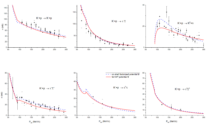
Figure 1: Elastic and inelastic $K^{-}p$ cross sections for the potentials $\bm{U}$ and $\bm{V}$.

More or less equal quality fits can be obtained for both potentials but for very different parameter values. This means, that $\hat{U}$ can not be considered as an approximation to $\hat{V}$ – they are basically different interactions. Their most significant difference is, that, while the full WT potential $\hat{V}$ produces a single pole in the region of $\Lambda(1405)$, the on-shell factorized potential $\hat{U}$ for any reasonable combination of parameters produces the familiar two poles. The pole positions for the two potentials are

$$\begin{split}z1&=(1425-21i)MeV\ \ {\rm for}\ \ \hat{V}\ \ {\rm and}\\ z1&=(1428-35i)MeV\ \ {\rm and}\ \ z2=(1384-62i)MeV\ \ {\rm for}\ \ \hat{U}.\end{split}$$

The position of the single $\hat{V}$ pole does not confirm the strong $K^{-}p$ binding, which is the main feature of the phenomenological potentials adjusted to the PDG pole position.

	$\hat{V}$	$\hat{U}$	Exp
$\gamma$	$2.32$	$2.35$	$2.36\pm 0.04$
$R_{c}$	$0.671$	$0.664$	$0.664\pm 0.011$
$R_{n}$	$0.202$	$0.194$	$0.189\pm 0.015$
$\Delta E\ (eV)$	$350-279\ i$	$302-294\ i$	$(283\pm 36)-(271\pm 46)\ i$

Table 1: Calculated and experimental values of the discrete data for potentials $\hat{U}$ and $\hat{V}$.

	$F_{\pi}$	$F_{K}$	$\beta_{1}$	$\beta_{2}$	$\beta_{3}$	$\beta_{4}$	$\beta_{5}$
$\hat{V}$	80.8	132	1094	960	516	537	629
$\hat{U}$	107	109	1247	1622	919	959	443

Table 2: Parameters of the potentials $\hat{V}$ and $\hat{U}$ (all values are given in $MeV$).

Most recent and accurate information on the $\Lambda(1405)$ resonance comes from the CLAS photoproduction experiment $\gamma+p\rightarrow K^{+}+\pi^{0}+\Sigma^{0}$ [3] in which the $M(\pi^{0}\Sigma^{0})$ missing mass spectra give the $\Lambda(1405)$ line shape. For the analysis of these spectra at present we have the semi-phenomenological final state interaction formula of Roca and Oset [4], which contains some adjustable parameters $c_{i}$ and the $T$-matrix elements of the $\bar{K}N-\pi\Sigma-\pi\Lambda$ potential. Using energy-dependent (two-pole) $\bar{K}N$ potentials, with simultaneous variation of $c_{i}$ and the potential parameters, acceptable fits to the CLAS data were obtained. This fact then was considered as the ultimate proof of the two-pole structure of the $\Lambda(1405)$.

Using the same formula (corrected for the repeated use of on-shell factorization), we have made a preliminary fit to the few lowest $\gamma$-energy bin CLAS data varying only the $c_{i}$-s with our unchanged single-pole potential $\hat{V}$. The results are shown in Fig.2.

It does not seem, that another pole is necessarily needed to improve these fits. A complete analysis of the CLAS data, including the charged channels is the subject of a forthcoming work.

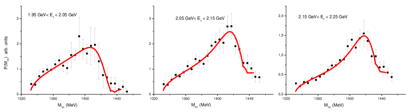
Figure 2: Fit to the first 3 $\gamma$-energy bins of CLAS $M(\pi^{0}\Sigma^{0})$ missing mass spectra in $\gamma+p\rightarrow K^{+}+\pi^{0}+\Sigma^{0}$ photoproduction.

Conclusions

• It was shown, that the energy-dependence of the WT term of the $\bar{K}N$ interaction, derived from the chiral $SU(3)$ Lagrangian and responsible for the appearance of a second pole in the $\Lambda(1405)$ region, follows from the unjustified application of the on-shell factorization approximation.

• Without this approximation a new, chiral based, energy-independent $\bar{K}N$ interaction was derived, which supports only one pole in the region of the $\Lambda(1405)$ resonance.

• The widely accepted ”two-pole structure” of the $\Lambda(1405)$ state thus becomes questionable.

• In coordinate space calculations for $n>2$ systems the use of the new potential avoids the not easily (and not uniquely) surmountable difficulties arising from the energy dependence of the two-body interaction.

The work was supported by the Hungarian OTKA grant 109462.

References

• [1] E. Oset, A. Ramos: Non-perturbative chiral approach to $s$-wave $\bar{K}N$ interactions. Nucl. Phys. A 635(1998)99
• [2] JΓ‘nos Revai: Are the chiral based $\bar{K}N$ potentials really energy-dependent? Few-Body Syst. 59(2018)49
• [3] K. Moriya et al. (CLAS collaboration): Measurement of the $\Sigma\pi$ photoproduction line shapes near the $\Lambda(1405)$ Phys. Rev. C 87(2013)035206
• [4] L. Roca, E. Oset : $\Lambda(1405)$ poles obtained from $\pi^{0}\Sigma^{0}$ photoproduction data Phys. Rev. C 87(2013)055201