Another look at recovering local homology from samples of stratified sets

Abstract.

Recovering homological features of spaces from samples has become one of the central themes of topological data analysis, leading to many successful applications. Many of the results in this area focus on global homological features of a subset of a Euclidean space. In this case, homology recovery predicates on imposing well understood geometric conditions on the underlying set. Typically, these conditions guarantee that small enough neighborhoods of the set have the same homology as the set itself. Existing work on recovering local homological features of a space from samples employs similar conditions locally. However, such local geometric conditions may vary from point to point and can potentially degenerate. For instance, the size of local homology preserving neighborhoods across all points of interest may not be bounded away from zero. In this paper, we introduce more general and robust conditions for local homology recovery and show that tame homology stratified sets, including Whitney stratified sets, satisfy these conditions away from strata boundaries, thus obtaining control over the regions where local homology recovery may not be feasible. Moreover, we show that true local homology of such sets can be computed from good enough samples using Vietoris-Rips complexes.

1. Introduction

Estimating topological features of a space from samples is one of the central topics in topological data analysis (TDA), which is a new field that has been steadily gaining popularity due to a series of successful applications [see e.g. 17, 6, 11, 7, 20]. The importance of such estimates stems from the fact that they provide us with a better insight into the process underlying the data, and can potentially help us select a better class of generative models. Much of the work within TDA focuses on developing and performing theoretical analyses of various methods for summarizing global homological properties of data sets. In particular, by imposing well understood geometric conditions on the underlying space, several guarantees for recovery of correct homology from sufficiently dense samples have been obtained [e.g. 22, 23, 10, 8].

Of course, one can easily make an argument that recovering global homological information may not be enough. Indeed, a space having the shape of the letter X is contractible, and thus has trivial homology, but the presence of a singular point may be extremely important. Many of such singular points can be captured through local homology, which suggests that collections containing local homological features across all the points in a sample may provide valuable information about the underlying space. Consequently, the need arises for theoretical results regarding such collections of local homological features. It is reasonable to expect that such results would require certain regularity conditions on the underlying space, and “nice” stratified spaces arise as a natural class of spaces that may possess the needed properties.

There have been several impressive efforts regarding recovery of local homological features of subsets of a Euclidean space from samples. Such results rely on the fact that if a set of interest is sufficiently nice, then the local homology is “well behaved”. The latter typically means that for all sufficiently small $\rho>0$ and all $\varepsilon>0$ which are sufficiently smaller than $\rho$, the following holds: the homology of the $\varepsilon$-neighborhood of the whole set relative to the part of the neighborhood outside of the ball of radius $\rho$ centered at a point of interest is isomorphic to the local homology at that point. In such a case, we say that the set has a positive local homological feature size at the point of interest. The size, $\varepsilon$, of the neighborhood of our set, as well as the radius, $\rho$, of the ball, are typically referred to as scales. By changing $\varepsilon$ and $\rho$ we obtain nested neighborhoods and balls along with the corresponding inclusion maps. The behavior of the induced homomorphisms on relative homology (with coefficients in a field) is typically summarized using persistent homology theory [15, 30], and may be referred to as multi-scale local homology. The true local homology is typically recovered from the multi-scale local homology by selecting appropriate scales.

The work in [2] focused on obtaining a multi-scale representation of local homology at a single point of a topologically stratified set. In particular, it was shown that the correct local homology at a single point can be inferred from a sufficiently good sample if the set has a positive local homological feature size at the point of interest. Later, the work in [3] described a local homology based method for assigning points of a noisy sample from a stratified set to their respective strata. It is important to note that theoretical guarantees for the correctness of such an assignment are based on local conditions, akin to the positive local homological feature size, imposed around pairs of points. It is also important to mention that the two previous results use Delaunay complexes for homology computations. These simplicial complexes have nice theoretical properties, but are computationally efficient only in low dimensions. The result in [29] focused on an efficient approximation of a multi-scale representation of local homology using Vietoris-Rips complexes. However, the authors of the latter paper do not address the question of when such an approximation captures the true local homology.

What one can take away from the above results is that the ability to recover local homology at a point relies on local geometric conditions (e.g. positivity of local homological feature size), which essentially determine the appropriate range of scales for our computations. Importantly, these conditions vary from point to point and may “degenerate”. For example, local homological feature size may not be bounded away from zero for a given set of points of interest, thus making the appropriate range of scales empty. This suggests that if one were to use the same scales to compute local homology at every point of a sample from a stratified set, some errors may be inevitable. It is important to be able to exercise control over the number of such errors. For a stratum of a stratified set, degeneration of the local geometric conditions guaranteeing local homology recovery is expected at the boundary. However, existing result do not address the question of whether such conditions do not degenerate away from the strata boundaries, and consequently do not provide a way to control errors.

It should be pointed out that the problem of recovering local homology simplifies significantly if the underlying space is a closed manifold. In fact, the result in [12] shows that the correct local homology of a closed submanifold of $\mathbb{R}^{n}$ can be recovered at any point of a noisy sample if the sample is close enough to the manifold in the Hausdorff metric. The goal of this paper, is to obtain a somewhat analogous result for a class of stratified sets that is large enough to subsume Whitney stratified sets. As we mentioned earlier, the main difficulty is in obtaining some control over the points where the recovery of the correct local homology cannot be guaranteed, and we propose an approach that allows us to tackle this issue. More specifically, we provide the following contributions:

1. We introduce a concept of local homological seemliness, with weak, moderate, and strong flavors, which generalizes the typically used concept of local homological feature size. Roughly speaking, the main difference between the two is that for local homological seemliness we no longer require the relative homology at small scales to be isomorphic to the true local homology – we only need the images of the inclusion induced homomorphisms between the relative homology at two sets of sufficiently small scales to be isomorphic to the true local homology. The reason for such a generalization is that Whitney stratified sets may fail to have positive homological feature size.

2. We show how local homology can be recovered from good enough samples of locally homologically seemly sets using Čech and Vietoris-Rips complexes. As we mentioned earlier, existing results do not show that the true local homology can be recovered using Vietoris-Rips complexes.

3. We prove that tame homology stratified sets as well as Whitney stratified sets are locally homologically seemly away from strata boundaries, thus obtaining some control over the region where mistakes are unavoidable. In particular, this result shows that with good enough samples, mistakes in recovering local homology of a stratum can happen only in a small region around its boundary.

4. We show how our results strengthen when the sets under consideration are nicer, e.g. have positive weak feature size or are manifolds (with or without boundary).

Two key results of the paper are stated in Theorems 2 and 3. These theorems also yield an important corollary. Suppose that $K\subset\mathbb{R}^{n}$ is a compact neighborhood retract possessing a Whitney stratification or, more generally, a tame homology stratification, $\mathcal{S}$. Let $P\subset\mathbb{R}^{n}$ be a finite set (a noisy sample of $K$). For $Q\subseteq P$, let $\mathcal{R}_{\alpha}(Q)$ denote the Vietoris-Rips complex at scale $\alpha$ over $Q$. Denote by $d_{H}$ the Hausdorff distance on compact subsets of $\mathbb{R}^{n}$. The corollary can be formulated as follows.

Corollary 1.

Let $\varepsilon>0$ be sufficiently small, and suppose that $d_{H}(P,K)<\varepsilon$. There are $\delta(\varepsilon)>0$, $R(\varepsilon)>r(\varepsilon)>0$, as well as strata dependent $w_{X}(\varepsilon)>0$, $X\in\mathcal{S}$, with $w_{X}(\varepsilon)\to 0$ as $\varepsilon\to 0$, such that for any $p\in P$, $x\in X\in\mathcal{S}$, and any homological dimensions $\ell$, the image of the inclusion induced homomorphism

$$H_{\ell}(\mathcal{R}_{\varepsilon}(P),\mathcal{R}_{\varepsilon}(P-B_{R(\varepsilon)}(p)))\to H_{\ell}(\mathcal{R}_{\delta(\varepsilon)}(P),\mathcal{R}_{\delta(\varepsilon)}(P-B_{r(\varepsilon)}(p)))$$

is isomorphic to the local homology $H(K,K-\{x\})$ as long as $\|x-p\|<\varepsilon$ and $\|x-y\|\geq w_{Y}(\varepsilon)$, where $Y$ is any stratum in the boundary of $X$ and $y\in Y$.

More details about the relevant concepts and the values of admissible scales are provided in subsequent sections. The corollary shows that even for fairly general stratified sets, we can compute correct local homology from samples for each stratum, except possibly for points close to the boundary of the strata. Moreover, we can do it efficiently using Vietoris-Rips complexes.

On the practical side, such results provide a justification for using Vietoris-Rips complexes when computing local homology, along with an additional insight into the range of applicable scales. A simple example is shown in Figure 1. The values of the quantities $\delta(\varepsilon)$, $r(\varepsilon)$ and $R(\varepsilon)$, as employed in Corollary 1, were chosen based on Corollary 3 in Section 3 and the estimate mentioned right after that corollary. These choices (implicitly) determine the values of $w_{Y_{1}}(\varepsilon)$ and $w_{Y_{2}}(\varepsilon)$, and we can see how they affect correctness of local homology estimation at the points along the $1$-dimensional strata that are too close to the boundary. In fact, Corollary 1 says that regardless of our choice of admissible scales, there may always be regions close to the $0$-dimensional strata where local homology estimation will fail. We would also like to point out that the cost of our computation would remain essentially the same even if we isometrically embedded the given stratified set in a very high dimensional Euclidean space. In contrast, such an embedding would make the use of Delaunay complexes computationally prohibitive.

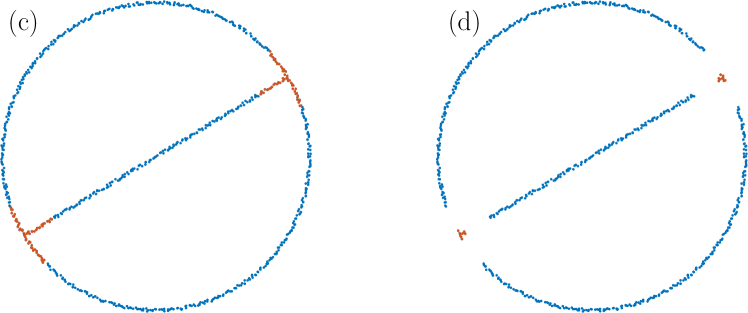
Figure 1. An example of recovering local homology from a sample of a stratified set using Vietoris-Rips complexes. (a) A simple stratified set, $K$, consisting of a unit circle and a chord passing through its center. (b) Strata of $K$, consisting of two open arcs, an open line segment, and two points. (c) An $\varepsilon$-sample of $K$, with $\varepsilon<0.019$. Blue and red colors indicate points where $1$-dimensional local homology was estimated to have rank $1$ and $2$, respectively. (d) The part of the sample where local homology was estimated correctly. To simplify the computation, coefficients in $\mathbb{Z}_{2}$ were used. The values for the scales of Vietoris-Rips complexes, as denoted in Corollary 1, were chosen as follows: $\delta(\varepsilon)=0.06$, $r(\varepsilon)=0.116$, $R(\varepsilon)=0.175$.

The rest of the paper is structured as follows. Section 2 provides background information along with some useful results, and introduces the classes of stratified sets that we shall be considering. In Section 3, we define the notions of a weak, moderate, and strong local homological seemliness. We also show that relative homology computed at points of an $\varepsilon$-sample of a locally homologically seemly stratified set using Vietoris-Rips or Čech complexes at certain scales recovers true local homology of the set at all points of the sample except for a small fraction. Section 4 is dedicated to proving that all the classes of stratified sets that we are considering, which include Whitney stratified sets, are locally homologically seemly, with stronger versions of seemliness for nicer sets. Section 5 concludes the paper. To improve the flow of the exposition, we moved the proofs of some technical lemmas to the Appendix.

2. Preliminaries

Before delving into the details of our exposition, we need to introduce some nomenclature and state a few useful results that we shall be relying upon later. We assume familiarity with basic algebraic topology, in particular homology theory, and refer the reader to such texts as [4, 13, 16], if a refresher on the subject is needed. A more complete background information on other relevant topics, e.g. the theory of stratified spaces and metric geometry, can be found in such comprehensive texts as [5, 25].

2.1. General notation and problem description

Throughout the paper, $(\mathbb{X},d)$ will denote a metric space, which we shall always assume to be complete and locally compact. We shall also assume that the metric $d$ is such that for any $x,y\in\mathbb{X}$ there is a midpoint, i.e. a point $z\in\mathbb{X}$ such that $d(x,y)=2d(x,z)=2d(y,z)$. Given $K\subseteq\mathbb{X}$, we denote by $\mathrm{cl}\left(K\right)$ the closure of $K$, by $\mathrm{int}\left(K\right)$ the interior of $K$, and by $K^{c}=\mathbb{X}-K$ the complement of $K$ in $\mathbb{X}$. Here and throughout the paper, the minus sign employed as a binary operation on sets denotes the usual set difference. It will be convenient to denote $\mathbb{R}^{n}_{+}=\{(x_{1},\ldots,x_{n})\in\mathbb{R}^{n}\,|\,x_{i}\geq 0,i=1,\ldots,n\}$. Given $\varepsilon\in\mathbb{R}_{+}$, we let

$$B_{\varepsilon}(K) =\{x\in\mathbb{X}\,|\,d(x,K)<\varepsilon\},$$

$$D_{\varepsilon}(K) =\{x\in\mathbb{X}\,|\,d(x,K)\leq\varepsilon\},$$

$$S_{\varepsilon}(K) =\{x\in\mathbb{X}\,|\,d(x,K)=\varepsilon\},$$

where $d(x,K)=\inf_{y\in K}{d(x,y)}$. Thus, for $x\in\mathbb{X}$, $B_{\varepsilon}(x)$, $D_{\varepsilon}(x)$, and $S_{\varepsilon}(x)$ denote the open ball, the closed ball, and the sphere of radius $\varepsilon$ centered at $x$, respectively. Throughout the paper, we shall adopt the convention $\inf{\emptyset}=\infty$ and $\sup{\emptyset}=-\infty$, which immediately implies that $D_{\varepsilon}(\emptyset)=B_{\varepsilon}(\emptyset)=\emptyset$ for $\varepsilon\in\mathbb{R}_{+}$.

The aforementioned assumptions on the metric space $(\mathbb{X},d)$ guarantee existence of shortest paths between any two points [5, Theorem 2.4.16]. We shall call a set $A\subseteq\mathbb{X}$ strongly convex if any two points $x,y\in A$ are connected by a unique shortest path lying completely in $A$ and depending continuously on the end points. The space $\mathbb{X}$ will be called locally strongly convex if all sufficiently small open (and hence closed) balls at any point are strongly convex. In particular, if $\mathbb{X}$ has curvature bounded from above then it is locally strongly convex [5, Proposition 9.1.17]. The convexity radius at $x\in\mathbb{X}$, denoted $\mathrm{conv}(x)$, is the supremum over all $\delta$ such that $B_{\delta}(x)$ is convex. The convexity radius of $K\subseteq\mathbb{X}$ is $\mathrm{conv}(K)=\inf\{\mathrm{conv}(x)\,|\,x\in K\}$. In a locally strongly convex space, $\mathrm{conv}(K)>0$ if $K$ is compact. For the rest of the paper, $\mathbb{X}$ will be assumed locally strongly convex.

If $\mathbb{X}$ is a Riemannian manifold and $M\subseteq\mathbb{X}$ is a submanifold, $T_{x}M$ will denote the tangent space to $M$ at $x\in M$. We will make use of the notion of transversality. Recall that two submanifolds $M,N\subseteq\mathbb{X}$ intersect transversally, denoted $M\pitchfork N$, if for any $x\in M\cap N$ we have $T_{x}M+T_{x}N=T_{x}\mathbb{X}$.

Let $K\subseteq\mathbb{X}$ be a compact set. We shall use the phrase local homology of $K$ at $x\in K$ to refer to the local singular homology groups of all homological dimensions. More specifically, we define $H(K,K-\{x\})=\bigoplus_{\ell}{H_{\ell}(K,K-\{x\})}$, with maps between such objects being direct sums of maps between the homology groups of each dimension. By local homology of $K$ we shall mean the collection $\{H(K,K-\{x\})|x\in K\}$. Throughout the paper, homology groups are assumed to have coefficients in $\mathbb{Z}$.

Our goal is to estimate (in a very broad sense) the local homology of $K$ when only an $\varepsilon$-sample of $K$ is available. Given $\varepsilon>0$, an $\varepsilon$-sample of $K$ is a finite set $P\subset\mathbb{X}$ such that $d_{H}(K,P)<\varepsilon$, where $d_{H}$ denotes the Hausdorff distance:

$$d_{H}(K,P)=\max\left\{\inf\{\delta>0\,|\,K\subseteq B_{\delta}(P)\}\right.,\left.\inf\{\delta>0\,|\,P\subseteq B_{\delta}(K)\}\right\}.$$

Such a $P$ is often called a noisy $\varepsilon$-sample, since we do not require $P\subseteq K$. If the latter condition is satisfied, we say that $P$ is noise-free. Note that for $\delta\geq 0$ we have

$$D_{\delta+\varepsilon}(P)\supseteq D_{\delta}(K)\quad\text{ and }\quad D_{\delta+\varepsilon}(P)-B_{r}(p)\supseteq D_{\delta}(K)-B_{R}(x),$$

where $p\in P$, $x=\operatorname*{arg\,min}_{z\in K}{d(p,z)}$, and $R\geq r+\varepsilon$. Thus, it is reasonable to expect that for a “sufficiently nice” set $K$, the relative homology groups $H(D_{a}(P),D_{a}(P)-B_{b}(p))$ (with appropriately chosen $b>a>0$) capture the local homology of $K$ at $x$. In what follows, it will be convenient to refer to the size, $\delta$, of a neighborhood $D_{\delta}(K)$ as a global scale, and to the radius of the ball $B_{R}(x)$ as a local scale.

2.2. A simple algebraic consideration

A majority of homology inference results in topological data analysis rely on the following simple observation: if a sequence of group isomorphisms,

$$A_{1}\to A_{2}\to A_{3},$$

factors through groups $B_{1}$ and $B_{2}$ to form a sequence

$$A_{1}\to B_{1}\to A_{2}\to B_{2}\to A_{3},$$

then the image of the resulting homomorphism from $B_{1}$ to $B_{2}$ is isomorphic to $A_{i}$, $\mathrm{im\,}{(B_{1}\to B_{2})}\approx A_{i}$, $i=1,2,3$. For example, if one can construct three nested neighborhoods of the set of interest $K$ which capture its true homology and interleave with two nested neighborhoods of the sample $P$, then the above result tells us that the correct homology can be recovered by looking at the image of the inclusion induced homomorphisms between the homology groups of the two neighborhoods of $P$.

We shall need a slight generalization of this observation.

Lemma 1.

Suppose that a sequence of group homomorphisms

$$A_{0}\overset{\varphi_{0}}{\to}A_{1}\overset{\varphi_{1}}{\to}A_{2}\overset{\varphi_{2}}{\to}A_{3}$$

factors through groups $B_{1}$ and $B_{2}$ to form a sequence

$$A_{0}\overset{\psi_{0}}{\to}B_{1}\overset{\psi_{1}}{\to}A_{1}\overset{\varphi_{1}}{\to}A_{2}\overset{\gamma}{\to}B_{2}\overset{\psi_{2}}{\to}A_{3},$$

and is such that restrictions $\mathrm{im\,}{\varphi_{i-1}}\to\mathrm{im\,}{\varphi_{i}}$, $i=1,2$, are isomorphisms. Then $\mathrm{im\,}{(B_{1}\to B_{2})}$ $\approx$ $\mathrm{im\,}{\varphi_{i}}$, $i=0,1,2$.

Proof.

Clearly, $\mathrm{im\,}{\varphi_{0}}=\mathrm{im\,}{\psi_{1}\circ\psi_{0}}\subseteq\mathrm{im\,}{\psi_{1}}$ and $\mathrm{im\,}{\varphi_{1}\circ\psi_{1}}\subseteq\mathrm{im\,}{\varphi_{1}}$, and since the restriction $\mathrm{im\,}{\varphi_{0}}\to\mathrm{im\,}{\varphi_{1}}$ is an isomorphisms, we get $\mathrm{im\,}{\varphi_{1}\circ\psi_{1}}=\mathrm{im\,}{\varphi_{1}}$. Also, the restriction $\mathrm{im\,}{\varphi_{1}}\to\mathrm{im\,}{\gamma}\circ\varphi_{1}$ is an isomorphisms because $\mathrm{im\,}{\varphi_{1}}\to\mathrm{im\,}{\varphi_{2}}$ is. Hence, $\mathrm{im\,}{(B_{1}\to B_{2})}=\mathrm{im\,}{\gamma\circ\varphi_{1}\circ\psi_{1}}\approx\mathrm{im\,}{\varphi_{1}}$. ∎

This result allows us to relax the requirement that (pairs of) nested neighborhoods of the set of interest $K$ (and a point $x\in K$) capture the true (local) homology – it is sufficient that the images of the inclusion induced homomorphisms capture it. More specifically, we need to look for nested neighborhoods $D_{\delta_{i}}(K)$, $B_{r_{i}}(x)$, $i=0,1,2,3$, with $\delta_{i}\leq\delta_{j}$ and $r_{i}\geq r_{j}$ for $i\leq j$, such that the images of homomorphisms

$$H(D_{\delta_{i}}(K),D_{\delta_{i}}(K)-B_{r_{i}}(x))\to H(D_{\delta_{j}}(K),D_{\delta_{j}}(K)-B_{r_{j}}(x)),\quad i<j,$$

are isomorphic to $H(K,K-\{x\})$. Then we can try to interleave these neighborhoods with the corresponding neighborhoods of the $\varepsilon$-sample $P$.

2.3. Čech and Vietoris-Rips complexes

When performing actual computations, one employs combinatorial structures which capture topology of the neighborhoods of interest. Two of such structures are the Čech and Vietoris-Rips simplicial complexes.

If $\mathbb{X}$ is a metric space, $P\subseteq\mathbb{X}$, and $\alpha>0$, the Čech complex over $P$ at a scale $\alpha$, $\mathcal{C}_{\alpha}(P)$, is an abstract simplicial complex consisting of (abstract) simplices, i.e. finite subsets, $\sigma\subseteq P$ such that $\cap_{x\in\sigma}{D_{\alpha}(x)}\neq\emptyset$. In other words, it is the nerve of the collection of balls $\{D_{\alpha}(x)\,|\,x\in P\}$ [see e.g. 16]. The Vietoris-Rips complex, $\mathcal{R}_{\alpha}(P)$, consists of all simplicies $\sigma\subseteq P$ whose edges belong to $\mathcal{C}_{\alpha}(P)$.

If $P$ is finite and the balls $D_{\alpha}(x)$, $x\in P$, are strongly convex, then $D_{\alpha}(P)$ and $\mathcal{C}_{\alpha}(P)$ are homotopy equivalent [see e.g. 14]. Vietoris-Rips complexes are generally not homotopy equivalent to the corresponding Čech complexes, but they are easier to construct and satisfy the following interleaving condition: $\mathcal{C}_{\alpha}(P)$ $\subseteq$ $\mathcal{R}_{\alpha}(P)$ $\subseteq$ $\mathcal{C}_{s\alpha}(P)$, where $s=2$ in general, and $s=\sqrt{\frac{2n}{n+1}}$ if $\mathbb{X}$ is an $n$-dimensional Euclidean space [see e.g. 11, Theorem 2.5]. If the dimension of the Euclidean space is not specified, one can safely take $s=\sqrt{2}$.

We shall use Čech and Vietoris-Rips complexes in the setting where $P$ is an $\varepsilon$-sample of a compact set $K\subseteq\mathbb{X}$. The goal is to recover the local homology at points of $K$ using the relative homology of appropriately chosen subcomplexes of the Čech and Vietoris-Rips complexes over $P$. The required scales for the simplicial complexes may differ depending on the type of the $\varepsilon$-sample (noisy or noise-free) and the space $\mathbb{X}$ (Euclidean space or not). Hence, it will be convenient to introduce two constants (depending on $P$ and $\mathbb{X}$, respectively) that capture these differences. Throughout the paper, we let

(1) $$t=\left\{\begin{aligned} 0,&\quad\text{ if }P\text{ is noise free},\\ 1,&\quad\text{ otherwise},\end{aligned}\right.\quad\quad s=\left\{\begin{aligned} \sqrt{2},&\quad\text{ if }\mathbb{X}\text{ is a Euclidean space},\\ 2,&\quad\text{ otherwise}.\end{aligned}\right.$$

It will also be convenient to introduce the some helpful notation for local and relative homology groups. Throughout the paper, we let

(2) $$F(a,b) =H(D_{a}(K),D_{a}(K)-B_{b}(x)),\quad\text{ for }a>0\text{ or }b>0,$$

$$F(0,0) =H(K,K-\{x\}),$$

$$C(a,b) =H(\mathcal{C}_{a}(P),\mathcal{C}_{a}(P-B_{b}(p))),$$

$$V(a,b) =H(\mathcal{R}_{a}(P),\mathcal{R}_{a}(P-B_{b}(p))).$$

The dependency of the left hand sides on points $p\in P$ and $x\in K$ has been suppressed, since it will be either stated or clear from the context how they should be chosen.

We now can state a lemma that lays a foundation for the subsequent use of Čech and Vietoris-Rips complexes.

Lemma 2.

Suppose that $K\subseteq\mathbb{X}$ is compact and $P\subset\mathbb{X}$ is an $\varepsilon$-sample of $K$. Let $p\in P$, and let $x\in K$ be a point closest to $p$. For $\delta\geq 0$, take

$$R>(1+s)\delta+(1+s+2t)\varepsilon,$$

and assume $s(\delta+\varepsilon)<\mathrm{conv}(P)$. Then inclusion induced homomorphisms

$$F(\delta,R)\to F(\beta_{c},r_{c})\quad\text{and}\quad F(\delta,R)\to F(\beta_{v},r_{v}),$$

where

$$\beta_{c}\geq\delta+(1+t)\varepsilon,\quad r_{c}\leq R-2\delta-(2+2t)\varepsilon,$$

$$\beta_{v}\geq s\delta+(s+t)\varepsilon,\quad r_{v}\leq R-(1+s)\delta-(1+s+2t)\varepsilon,$$

factor through

$$C(\delta+\varepsilon,r+\delta+(1+t)\varepsilon)\quad\text{and}\quad V(\delta+\varepsilon,r+s\delta+(s+t)\varepsilon),$$

respectively:

(3)

(4)

Proof.

Note that if $P\subseteq K$ then $p=x$, so we have $B_{b}(x)$ $\supseteq$ $B_{b-t\varepsilon}(p)$. The triangle inequality also yields

$$D_{a}(K)\subseteq D_{a+\varepsilon}(P)\subseteq D_{a+(1+t)\varepsilon}(K),$$

$$D_{a}(P)-B_{b}(p)\subseteq D_{a}(P-B_{b-a}(p))\subseteq D_{a}(P)-B_{b-2a}(p).$$

Since $\mathcal{C}_{\alpha}(Q)$ is homotopy equivalent to $D_{\alpha}(Q)$ for any $Q\subseteq P$, $\alpha<\mathrm{conv}(P)$, the five-lemma [see e.g. 4, Lemma 5.10] yields $H(\mathcal{C}_{\alpha}(P),\mathcal{C}_{\alpha}(Q))$ $\approx$ $H(D_{\alpha}(P),D_{\alpha}(Q))$. Denoting

$$G(a,b) =H(D_{a}(P),D_{a}(P)-B_{b}(p)),$$

$$J(a,b) =H(D_{a}(P),D_{a}(P-B_{b}(p))),$$

and noting that $r_{c}+\delta+(1+t)\varepsilon$ $\leq$ $R-\delta-(1+t)\varepsilon$ we obtain

which implies (3). Note that it is enough to have $\delta+\varepsilon<\mathrm{conv}(K)$ for this result to hold.

Taking into account that $\mathcal{C}_{\alpha}(Q)$ $\subseteq$ $\mathcal{R}_{\alpha}(Q)$ $\subseteq$ $\mathcal{C}_{s\alpha}(Q)$ for any $Q\subseteq P$, we obtain

which implies (4). ∎

It is worth mentioning that, in the above lemma, the noisy case does not require $x$ to be the closest point – we simply need $d(x,p)<\varepsilon$. Also, we can notice that the amounts by which the scales of the complexes and the radii of the balls have to change follow a certain pattern. More specifically, the quantities that stand out are $c\delta+(c+t)\varepsilon$ and $(1+c)\delta+(1+c+2t)\varepsilon$, where $c$ is equal to either $1$ or $s$. Since we may need to employ these kind of quantities multiple times, we introduce the notation

(5) $$g_{c}(a,b) =ca+(c+t)b,$$

$$f_{c}(a,b) =g_{c}(a,b)+g_{1}(a,b)=$$

$$=(1+c)a+(1+c+2t)b,\quad\quad\quad\quad c\in\{1,s\},$$

which will be used throughout the paper.

2.4. Stratified sets

To ensure a feasibility of the above approach to local homology recovery, at least for small enough $\varepsilon$, we need to impose some restrictions on the set $K$, and on the way $K$ is embedded in $\mathbb{X}$. To address the latter, we shall assume that $K$ is a neighborhood retract, that is, there is a neighborhood $U\supseteq K$ and a continuous map $\pi:U\to K$ such that $\pi(x)=x$ for all $x\in K$. As for $K$ itself, we shall require that it admit a tame homology stratification. By a stratification of $K$ we mean a locally finite collection $\mathcal{S}$ of pairwise disjoint, locally closed subsets of $K$ such that $K=\cup_{X\in\mathcal{S}}{X}$ and the Frontier Condition is satisfied:

$$\text{for all }X,Y\in\mathcal{S},X\cap\mathrm{cl}\left(Y\right)\neq\emptyset\implies X\subseteq\mathrm{cl}\left(Y\right).$$

A set $X\in\mathcal{S}$ is called a stratum. A stratification $\mathcal{S}$ is a tame homology stratification if it satisfies the following conditions:

1. Each $X\in\mathcal{S}$ is a finite dimensional homology manifold. That is, for any $x\in X$, $H_{\ell}(X,X-\{x\})$ is trivial for all $\ell\geq 0$ except one – the dimension of $X$ – in which case it is isomorphic to $\mathbb{Z}$.

2. For any $x\in X\in\mathcal{S}$, the inclusion induced homomorphisms

   $$H_{\ell}(K,K-B_{r}(x))\to H_{\ell}(K,K-\{x\}),\text{ and}$$

   $$H_{\ell}(K,K-B_{r}(x))\to H_{\ell}(K,K-B_{\rho}(y))\to H_{\ell}(K,K-\{y\})$$

   are all isomorphisms as long as $r>0$ is sufficiently small, $y\in B_{r}(x)\cap X$, and $0<\rho<r-d(x,y)$. Moreover, each $H_{\ell}(K,K-\{x\})$, $\ell\geq 0$, is finitely generated.

Note that these conditions imply that local homology groups remain constant along the strata. We shall consider only tame homology stratifications, and will omit the qualifier “tame” for convenience.

Assume now that a set $K\subseteq\mathbb{X}$ is endowed with a stratification $\mathcal{S}$. The Frontier Condition induces a partial order on the stratification: given $X,Y\in\mathcal{S}$, we define $X\leq Y$ if $X\subseteq\mathrm{cl}\left(Y\right)$. It follows that for each $Y\in\mathcal{S}$ we have $\mathrm{cl}\left(Y\right)=\cup_{X\leq Y}{X}$. We say that a stratum $X\in\mathcal{S}$ has height $k$, and denote it by $0pt{X}=k$, if $k$ is the largest integer such that there exist $X_{0},\ldots,X_{k}\in\mathcal{S}$ satisfying $X_{0}\leq\cdots\leq X_{k}=X$. In other words, the height of $X\in\mathcal{S}$ is one less than the size of the longest chain in $\mathcal{S}$ having $X$ as the maximal element. As an example, consider the stratification shown in Figure 1(b). It has two strata of height $0$ and three strata of height $1$. We shall denote by $\mathcal{S}_{k}$ the collection of all the strata of height $k$, that is, $\mathcal{S}_{k}=\{X\in\mathcal{S}\,|\,0pt{X}=k\}$. Clearly, every minimal element of $\mathcal{S}$ has height zero, so $\mathcal{S}_{0}$ contains all the minimal elements.

Suppose we have another metric space $\mathbb{Y}$ and a set $L\subseteq\mathbb{Y}$ with a stratification $\mathcal{R}$. We say that a map $f:\mathbb{X}\to\mathbb{Y}$ is stratum preserving (or stratified) if $f(K^{c})\subseteq L^{c}$, and for any $X\in\mathcal{S}$ there is $Y\in\mathcal{R}$ such that $f(X)\subseteq Y$. Similarly, given a (not necessarily stratified) set $A\subseteq\mathbb{Y}$ and a map $F:A\times[0,1]\to\mathbb{X}$, we say that $F$ is stratum preserving if for any $x\in A$ either $F(\{x\}\times[0,1])\subseteq K^{c}$ or there is $X\in\mathcal{S}$ such that $F(\{x\}\times[0,1])\subseteq X$. We say that $F$ is nearly stratum preserving if it is stratum preserving on $A\times[0,1)$.

Existence of a homology stratification of $K$ implies only very mild restrictions on the geometric behavior of the neighborhoods of strata in $K$. One could make those restrictions a little stronger by requiring strata to be (topological) manifolds satisfying certain homotopy based or homeomorphism based compatibility conditions, as do the homotopically stratified spaces of Quinn [27] or the locally cone-like TOP stratified sets of Siebennman [28]. However, it will be more instructive to investigate how local homology recovery improves when significantly stronger geometric restrictions on the strata are imposed.

Perhaps the most well known class of “nice” stratified sets are Whitney stratified sets. In this case, we assume $\mathbb{X}$ to be a smooth, complete Riemannian manifold. A stratification $\mathcal{S}$ of a set $K\subseteq\mathbb{X}$ is called a Whitney stratification if each stratum is a smooth manifold, and for any two strata $Y\leq X$ the following conditions hold: whenever $x_{i}\in X$ and $y_{i}\in Y$ are two sequences converging to $y\in Y$ such that the tangent spaces $T_{x_{i}}X$ converge (in the corresponding Grasmannian) to a space $\tau$, and (with respect to some local coordinate system on $\mathbb{X}$) the secant lines $l_{i}=\overline{x_{i}y_{i}}$ converge (in the corresponding projective space) to a line $l$, we have

• $T_{y}Y\subseteq\tau$

• $l\subseteq\tau$.

Stratified sets satisfying the above condition (a) or (b) are called (a)-regular or (b)-regular, respectively. It is well know that (b)$\implies$(a) [see e.g. 21]. If $K\subset\mathbb{X}$ is a Whitney stratified set, it may be useful to employ a uniform view and regard the manifold $\mathbb{X}$ as a Whitney stratified set whose strata are $\mathbb{X}-K$ and the strata of $K$.

Besides also being homology stratified, Whitney stratified sets have a lot of important properties [18, 25]. Pertinent to our problem is the fact that if $\mathcal{S}$ is a Whitney stratification of a set $K\subseteq\mathbb{X}$ and $L\subseteq K$ is a closed union of strata, then there exists a neighborhood $U\supseteq L$ in $\mathbb{X}$ and a nearly stratum preserving continuous map $F:U\times[0,1]\to U$ providing a strong deformation retraction of $U$ onto $L$, i.e., $F(x,0)=x$ and $F(x,1)\in L$ for $x\in U$, $F(y,t)=y$ for $y\in L$, $t\in[0,1]$ (see e.g. [26] as well as Theorem 3.9.4 in [25]). Another useful fact concerns transverse intersections and unions of Whitney stratified sets. If $\mathcal{S}$ and $\mathcal{R}$ are Whitney stratifications of subsets $K,L\subseteq\mathbb{X}$, respectively, we say that $K$ intersects $L$ transversely if $X$ intersects $Y$ transversally for any $X\in\mathcal{S}$, $Y\in\mathcal{R}$. In such a case, the stratification

$$\mathcal{S}\cap_{t}\mathcal{R}=\cup{\{X\cap Y\}},$$

where the union is taken over all $X\in\mathcal{S}$ and $Y\in\mathcal{R}$ with non-empty intersection, is a Whitney stratification of $K\cap L$ [see e.g. 9]. In other words, a transverse intersection of two Whitney stratified sets is a Whitney stratified set whose strata are intersections of the strata of the two sets. Let us define

$$\mathcal{S}\cup_{t}\mathcal{R}=\bigcup\big{(}\{X\cap Y\}\cup\{X-Y\}\cup\{Y-X\}\big{)},$$

where the union is taken over all $X\in\mathcal{S}$ and $Y\in\mathcal{R}$ with non-empty intersection. The proof of the following lemma can be found in the Appendix.

Lemma 3.

Let $K,L\subseteq\mathbb{X}$ be two Whitney stratified sets with stratifications $\mathcal{S}$ and $\mathcal{R}$, respectively. Suppose that $K$ and $L$ intersect transversely. Then $K\cup L$ is a Whitney stratified set with stratification $\mathcal{S}\cup_{t}\mathcal{R}$.

Thus, the union of two transversely intersecting Whitney stratified sets is a Whitney stratified set whose strata are the intersections and the differences of the strata of the two sets.

2.5. Distance function and weak feature size

An alternative way to impose some geometric regularity on a compact set $K\subset\mathbb{X}$ is through the properties of the distance function

$$d_{K}:\mathbb{X}\to\mathbb{R}_{+},\quad d_{K}(x)=\inf_{y\in K}{d(x,y)}.$$

Assuming that $\mathbb{X}$ is a smooth Riemannian manifold, a point $x\in\mathbb{X}-K$ is called regular for $d_{K}$ if there is a unit vector $v\in T_{x}\mathbb{X}$ such that for any shortest unit speed geodesic $\gamma$ connecting $x$ to the set of closest points in $K$, we have $\angle(v,\dot{\gamma}(0))>\frac{\pi}{2}$ [see e.g. 19, 24]. Otherwise, $x$ is a critical point, and the value $r\in\mathbb{R}_{+}$ is called critical if $d_{K}^{-1}(r)$ contains a critical point. The weak feature size of $K$, $\mathrm{wfs}(K)$, is the infimum of all positive critical values of $d_{K}$. If $\mathrm{wfs}(K)>0$, that is, there exists $\varepsilon>0$ such that $d_{K}^{-1}((0,\varepsilon))$ contains only regular points, then $D_{\delta_{1}}(K)=d_{K}^{-1}([0,\delta_{1}])$ is isotopic to $D_{\delta_{2}}(K)=d_{K}^{-1}([0,\delta_{2}])$ for any $\delta_{1},\delta_{2}\in(0,\varepsilon)$ [19]. Note that a Whitney stratified set may not have a positive weak feature size. Also, a compact set with a positive weak feature size may not admit a Whitney stratification. Thus, it may be reasonable to combine the two conditions and consider Whitney stratified sets which have a positive weak feature size.

3. Homological seemliness

Let us now fix a compact homology stratified neighborhood retract $K\subseteq\mathbb{X}$ with a stratification $\mathcal{S}$. First, we try to determine conditions that allow us to find nested neighborhoods of $K$ and a fixed $x\in K$ which can be used with Lemmas 1 and 2. We later show show that analogous conditions can be obtained for all of $K$, and that these conditions do hold under the assumptions that we made regarding $K$ and $\mathbb{X}$.

In addition to the assumptions on $K$ and $\mathbb{X}$, this section will rely on notation (1), (2), and (5), introduced in Section 2. Also, $P$ will always denote an $\varepsilon$-sample of $K$, $p\in P$ will be an arbitrary point, and, where appropriate, $x\in K$ will be either a point with $d(x,p)<\varepsilon$, if $P$ is noisy, or the closest point to $p$, if $P$ is noise-free. Any additional restrictions on $x$ will be states explicitly.

3.1. Homological seemliness at a point

Given $\varepsilon\in\mathbb{R}_{+}$, let $A(\varepsilon)=\{(R,r,\alpha)\in\mathbb{R}^{3}_{+}|R\geq r>\alpha\geq\varepsilon\}\subset\mathbb{R}^{3}_{+}$. For $x\in K$ we define $A_{x}(\varepsilon)$ as the set of all triples $(R,r,\alpha)\in A(\varepsilon)$ which satisfy the following conditions:

1. For all $\rho\in(0,R]$, $D_{\rho}(x)$ are topological balls (and $S_{\rho}(x)$ are transverse to all the strata, if $K$ is a Whitney stratified set).

2. Inclusions yield the commutative diagram

   (6)

Note that the above diagram imposes constraints on the triples $(R,r,\alpha)$ by requiring that certain inclusion induced homomorphisms be isomorphisms. The presence of the diagonal arrow in diagram (6) is equivalent to saying that $i_{*}$ is injective and the restriction $\mathrm{im\,}{i_{*}}\to\mathrm{im\,}{j_{*}}$ is an isomorphism. In the case $\varepsilon=0$, the imposed constraints imply that $A_{x}(0)$ contains triples $(R,r,\alpha)$ such that inclusion induced homomorphisms

$$H(K,K-B_{\rho}(x))\to H(D_{\alpha}(K),D_{\alpha}(K)-B_{\rho}(x)),\quad\rho\in[r,R],$$

are injective (with images isomorphic to the true local homology at $x$).

Intuitively, one can regard the sets $A_{x}(\varepsilon)$ as containing admissible global and local scales that can potentially be used with Lemmas 1 and 2. Indeed, suppose $(R,r,\alpha)\in A_{x}(\varepsilon)$. Then any spurious homology classes present in $H(D_{\varepsilon}(K)$, $D_{\varepsilon}(K)$ $-$ $B_{R}(x))$ disappear once we increase the global scale to $\alpha$ and decrease the local scale to $r$. This makes the use of Lemma 1 feasible. To see how to transform the mere feasibility into an actual result, we need to better understand the structure of $A_{x}(\varepsilon)$.

We start with the simple case $\varepsilon=0$. As an example, we explicitly computed the set $A_{x}(0)$ for the simple stratified set from Figure 1, with $x$ a $0$-dimensional stratum. It is shown in Figure 2. More generally, we can prove the following result.

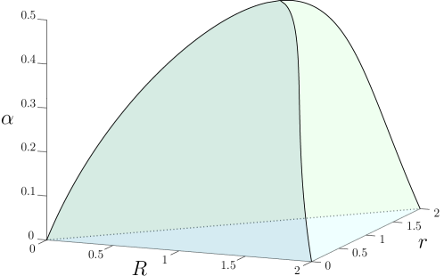
Figure 2. The structure of $A_{x}(0)$ for the stratified set from Figure 1.

Lemma 4.

For a sufficiently small $\alpha^{\prime}>0$, the sets of local scales

$$A_{x}(0\,|\,\alpha=\alpha^{\prime})=\{(R,r)\,|\,(R,r,\alpha^{\prime})\in A_{x}(0)\}$$

is not empty and has the structure of a right isosceles triangle (possibly not containing its legs) in the $(R,r)$-plane with the legs parallel to the axes, and the hypotenuse lying on the diagonal. Moreover, if $\alpha^{\prime}_{1}\leq\alpha^{\prime}_{2}$ then

$$A_{x}(0\,|\,\alpha=\alpha^{\prime}_{2})\subseteq A_{x}(0\,|\,\alpha=\alpha^{\prime}_{1}).$$

The proof of Lemma 4 can be found in the Appendix. The lemma suggests that the structure of $A_{x}(\varepsilon)$ may be understood through the structure of the sets

$$A_{x}(\varepsilon\,|\,\alpha=\alpha^{\prime})=\{(R,r)\,|\,(R,r,\alpha^{\prime})\in A_{x}(\varepsilon)\},$$

which we shall refer to as $\alpha$-sections.

It turns out that the structure of $A_{x}(\varepsilon)$ for $\varepsilon>0$ is only slightly more complicated than the structure of $A_{x}(0)$, and can be nicely described by considering the sections of $A_{x}(\varepsilon)$ by lines parallel to the coordinate axes. More specifically, we define

$$A_{x}(\varepsilon\,|\,R=R^{\prime},r=r^{\prime}) =\{\alpha\in\mathbb{R}_{+}|(R^{\prime},r^{\prime},\alpha)\in A_{x}(\varepsilon)\},$$

$$A_{x}(\varepsilon\,|\,R=R^{\prime},\alpha=\alpha^{\prime}) =\{r\in\mathbb{R}_{+}|(R^{\prime},r,\alpha^{\prime})\in A_{x}(\varepsilon)\},$$

$$A_{x}(\varepsilon\,|\,r=r^{\prime},\alpha=\alpha^{\prime}) =\{R\in\mathbb{R}_{+}|(R,r^{\prime},\alpha^{\prime})\in A_{x}(\varepsilon)\}.$$

We shall refer to these sets as line sections of $A_{x}(\varepsilon)$.

Lemma 5.

1. $A_{x}(\varepsilon)\subseteq A_{x}(\delta)$ whenever $0\leq\delta\leq\varepsilon$;

2. Line sections of $A_{x}(\varepsilon)$ are (possibly degenerate) intervals.

3. Suppose $(R_{1},r_{1},\alpha_{1})\in A_{x}(\varepsilon)$, and let $R_{2}>R_{1}$, $r_{2}<r_{1}$. Then

   $$A_{x}(\varepsilon|R=R_{1},\alpha=\alpha_{1})\subseteq A_{x}(\varepsilon|R=R_{2},\alpha=\alpha_{1}),$$

   $$A_{x}(\varepsilon|r=r_{1},\alpha=\alpha_{1})\subseteq A_{x}(\varepsilon|r=r_{2},\alpha=\alpha_{1})$$

   as long as the corresponding right hand side is not an empty set.

4. The above properties are preserved under intersections.

The proof of Lemma 5 can be found in the Appendix. The lemma implies that $\alpha$-sections $A_{x}(\varepsilon|\alpha=\alpha^{\prime})$ have a structure reminiscent of a right isosceles triangle. More specifically, if

$$R_{u} =\sup\{R\,|\,\exists r:(R,r)\in A_{x}(\varepsilon|\alpha=\alpha^{\prime})\},$$

$$R_{l} =\inf\{R\,|\,\exists r:(R,r)\in A_{x}(\varepsilon|\alpha=\alpha^{\prime})\},$$

$$r_{u} =\sup\{r\,|\,\exists R:(R,r)\in A_{x}(\varepsilon|\alpha=\alpha^{\prime})\},$$

$$r_{l} =\inf\{r\,|\,\exists R:(R,r)\in A_{x}(\varepsilon|\alpha=\alpha^{\prime})\},$$

then it is the set bounded by the line segment connecting points $(R_{l},r_{l})$ and $(R_{u},r_{l})$, another line segment connecting $(R_{u},r_{l})$ and $(R_{u},r_{u})$, and a curve connecting $(R_{l},r_{l})$ and $(R_{u},r_{u})$, and such that it is a graph (in the $(R,r)$-plane) of a non-decreasing function $f:[R_{l},R_{u}]\to[r_{l},r_{u}]$. We should note that this set may not contain (parts of) its boundary. An example of a possible structure of an $\alpha$-section is shown in Figure 3.

Looking back at Lemma 2, we see that the ability to interleave neighborhood of the form $(D_{\varepsilon}(K)$, $D_{\varepsilon}(K)$ $-$ $B_{\rho}(x))$ with the appropriate Čech or Vietoris-Rips complexes (so that Lemma 1 can be invoked) requires a certain range of local scales at appropriately chosen global scales. More specifically, starting with $(K,K-B_{R}(x))$ (and an $\varepsilon$-sample) we need to increase the global scale and decrease the local scale by some minimum amounts, so that an appropriate simplicial complex can be fit in between. This results in a global scale $\alpha_{1}$, and a local scale $\rho_{1}$. These scales need to be changed further to kill any spurious homology that could have been created, thus leading to scales $\alpha_{2}\geq\alpha_{1}$, $\rho_{2}\leq\rho_{1}$. The choice of the next scale levels, $\alpha_{3}$ and $\rho_{3}$, has to be done so that we, again, can fit our simplicial complex (at a larger scale) as well as destroy any spurious homology born at the previous scale levels.

The above procedure mandates that, at least for small $\varepsilon$, the sets $A_{x}(\varepsilon)$ contain a sufficiently large range of $\alpha$-sections, each including a sufficiently large range of local scales. To formalize these ideas, we denote a range of $\alpha$-sets by

$$A_{x}(\varepsilon\,|\,\alpha\in[\alpha_{1},\alpha_{2}])=\{(R,r,\alpha)\in A_{x}(\varepsilon)\,|\,\alpha\in[\alpha_{1},\alpha_{2}]\},$$

call it an $\alpha$-slab, and introduce the following definition.

Definition 1.

The collection of sets $A_{x}(\varepsilon)$, $\varepsilon\geq 0$, is called weakly seemly if there are $\varepsilon_{x}>0$ and functions $\alpha_{x}^{l},\alpha_{x}^{u}:[0,\varepsilon_{x}]\to\mathbb{R}_{+}$ satisfying the following:

1. $\alpha_{x}^{l}$ is non-decreasing and $\alpha_{x}^{u}$ is non-increasing;

2. $\alpha_{x}^{l}(\varepsilon)\searrow 0=\alpha_{x}^{l}(0)$ and $\alpha_{x}^{u}(\varepsilon)\nearrow\alpha_{x}^{u}(0)$ as $\varepsilon\to 0$;

3. $A_{x}(\varepsilon\,|\,\alpha=\alpha^{\prime})\neq\emptyset$ for all $\alpha^{\prime}\in[\alpha_{x}^{l}(\varepsilon),\alpha_{x}^{u}(\varepsilon)]$;

4. $\displaystyle\sup_{\alpha^{\prime}\in[\alpha_{x}^{l}(\varepsilon),\alpha_{x}^{u}(\varepsilon)]}{d_{H}(A_{x}(0\,|\,\alpha=\alpha^{\prime}),A_{x}(\varepsilon\,|\,\alpha=\alpha^{\prime}))}\to 0\quad\text{as}\quad\varepsilon\to 0.$

In this case, we also say that $K$ is weakly homologically seemly at $x$.

Recalling the structure of $A_{x}(0)$, we see that if $A_{x}(\varepsilon)$ is weakly seemly then for all sufficiently small $\varepsilon$ there is a non-shrinking $\alpha$-slab with $\alpha$-sections that are very close to right isosceles triangles of Lemma 4. Assuming weak seemliness, in which case we only consider $\varepsilon\in[0,\varepsilon_{x}]$, let us define

$$A_{x}([0,\varepsilon]\,|\,\alpha\leq\beta)=\bigcap_{\varepsilon^{\prime}\in[0,\varepsilon]}{\bigcap_{\alpha^{\prime}\in[\alpha_{x}^{l}(\varepsilon^{\prime}),\beta]}{A_{x}(\varepsilon^{\prime}\,|\,\alpha=\alpha^{\prime})}},$$

where $\beta\in[\alpha_{x}^{l}(\varepsilon),\alpha_{x}^{u}(\varepsilon)]$. This is the intersection of all $\alpha$-sections of $A_{x}(\varepsilon^{\prime})$ between $\alpha_{x}^{l}(\varepsilon^{\prime})$ and $\beta$ for all $\varepsilon^{\prime}\in[0,\varepsilon]$. It has the structure of a typical $\alpha$-section, and if $\varepsilon$ is sufficiently small, it is close to a right isosceles triangle. To better quantify the difference between the two, we define

$$\bar{R}_{x}(\varepsilon,\beta) =\sup\{R\,|\,\exists r:(R,r)\in A_{x}([0,\varepsilon]\,|\,\alpha\leq\beta)\},$$

$$\bar{r}_{x}(\varepsilon,\beta) =\inf\{r\,|\,\exists R:(R,r)\in A_{x}([0,\varepsilon]\,|\,\alpha\leq\beta)\}.$$

In addition, we denote by $\Delta_{x}(\varepsilon,\beta,\delta)$ the interior of the triangle with vertices

$$(\bar{r}_{x}(\varepsilon,\beta)+\delta,\bar{r}_{x}(\varepsilon,\beta)),(\bar{R}_{x}(\varepsilon,\beta),\bar{r}_{x}(\varepsilon,\beta)),(\bar{R}_{x}(\varepsilon,\beta),\bar{R}_{x}(\varepsilon,\beta)-\delta),$$

and let

$$\bar{\delta}_{x}(\varepsilon,\beta)=\inf\{\delta>0\,|\,\Delta_{x}(\varepsilon,\beta,\delta)\subseteq A_{x}([0,\varepsilon]\,|\,\alpha\leq\beta)\}.$$

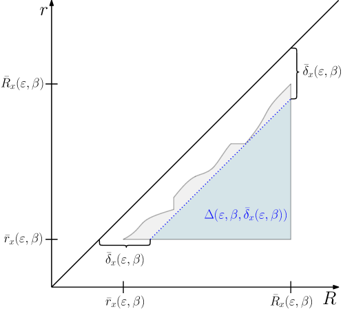
Figure 3. An example of the structure of $A_{x}([0,\varepsilon]\,|\,\alpha\leq\beta)$, which is also the structure of an $\alpha$-section.

A possible structure of $A_{x}([0,\varepsilon]\,|\,\alpha\leq\beta)$, along with the above defined quantities, is shown in Figure 3. We now see that the range of local scales at all the $\alpha$-sections (below $\beta$) is determined by the quantity

$$\tau_{x}(\varepsilon,\beta)=\bar{R}_{x}(\varepsilon,\beta)-\bar{r}_{x}(\varepsilon,\beta)-\bar{\delta}_{x}(\varepsilon,\beta),$$

which is the length of the side of the largest right isosceles triangle whose interior lies completely in $A_{x}([0,\varepsilon]\,|\,\alpha\leq\beta)$. As we mentioned in our earlier discussion, we would like $\tau_{x}(\varepsilon,\beta)$ to be sufficiently large for appropriately chosen $\varepsilon$ and $\beta$, as dictated by Lemma 2. Recalling quantities $f_{c}(a,b)$ and $g_{c}(a,b)$ from (5), we let $f(a,b)$ and $g(a,b)$ be continuous functions which decrease to zero as $a,b$ $\to$ $0$. We define

(7) $$E_{x}(f,g)=\left\{\varepsilon\,\left|\,\begin{aligned} &\tau_{x}(\varepsilon^{\prime},\beta)>\gamma,\,\varepsilon^{\prime}=\alpha_{x}^{l}(g(0,\varepsilon)),\\ &\beta=g(\varepsilon^{\prime},\varepsilon),\,\gamma=f(0,\varepsilon)+f(\varepsilon^{\prime},\varepsilon)\end{aligned}\right.\right\}$$

The set $E_{x}(f,g)$ and quantities $\tau_{x}(\varepsilon,\beta)$, $\bar{R}_{x}(\varepsilon,\beta)$, $\bar{r}_{x}(\varepsilon,\beta)$, and $\bar{\delta}_{x}(\varepsilon,\beta)$ have some useful properties. We list them in the following lemma, whose proof is given in the Appendix.

Lemma 6.

Suppose that $A_{x}(\varepsilon)$ is weakly seemly. Then the following holds:

1. If $\varepsilon_{1}\leq\varepsilon_{2},$ and $\beta_{1}\leq\beta_{2}$ then

   $$\bar{r}_{x}(\varepsilon_{1},\beta_{1}) \leq\bar{r}_{x}(\varepsilon_{2},\beta_{2}),\quad\bar{R}_{x}(\varepsilon_{1},\beta_{1})\geq\bar{R}_{x}(\varepsilon_{2},\beta_{2}),$$

   $$\bar{\delta}_{x}(\varepsilon_{1},\beta_{1}) \leq\bar{\delta}_{x}(\varepsilon_{2},\beta_{2}),\quad\tau_{x}(\varepsilon_{1},\beta_{1})\leq\tau_{x}(\varepsilon_{2},\beta_{2}).$$

2. $\bar{\delta}_{x}(\varepsilon,\beta)\to 0$ as $\varepsilon\to 0$ for all $\beta\in(0,\alpha_{x}^{u}(0))$. Also, $\bar{r}_{x}(\varepsilon,\beta)\to 0$ as $\varepsilon,\beta\to 0$.

3. $E_{x}(f,g)$ is a non-empty interval.

It is also useful to note that if $\varepsilon\in E_{x}(f,g)$ then $\Delta_{x}(\varepsilon^{\prime},\beta,\bar{\delta}_{x}(\varepsilon^{\prime},\beta)+\gamma)\neq\emptyset,$ where we retained the notation from (7).

Keeping in mind the assumptions and notation stated at the beginning of the section, we can now prove the following theorem.

Theorem 1.

Suppose that $K$ is weakly homologically seemly, $\varepsilon\in E_{x}(f_{c},g_{c})$, and $c(\varepsilon^{\prime}+\varepsilon)<\mathrm{conv}(P)$, where $\varepsilon^{\prime}=\alpha_{x}^{l}(g_{c}(0,\varepsilon))$. Let

$$\beta=g_{c}(\varepsilon^{\prime},\varepsilon),\quad\gamma=f_{c}(0,\varepsilon)+f_{c}(\varepsilon^{\prime},\varepsilon).$$

Then for all

$$(R^{\prime},r^{\prime})\in\Delta_{x}(\varepsilon^{\prime},\beta,\bar{\delta}_{x}(\varepsilon^{\prime},\beta)+\gamma),$$

and

$$R=R^{\prime}-g_{1}(0,\varepsilon),\quad r=r^{\prime}+g_{c}(\varepsilon^{\prime},\varepsilon),$$

we have

$$\mathrm{im\,}\big{(}C(\varepsilon,R)\to C(\varepsilon^{\prime}+\varepsilon,r)\big{)} \approx H(K,K-\{x\}),\quad c=1$$

$$\mathrm{im\,}\big{(}V(\varepsilon,R)\to V(\varepsilon^{\prime}+\varepsilon,r)\big{)} \approx H(K,K-\{x\}),\quad c=s$$

Proof.

The conditions of the lemma imply that all $\alpha$-sections below $\beta$ in any $A_{x}(\tilde{\varepsilon})$, $\tilde{\varepsilon}\in[0,\varepsilon^{\prime}]$, contain $\Delta_{x}(\varepsilon^{\prime},\beta,\bar{\delta}_{x}(\varepsilon^{\prime},\beta))$, and the side length of this triangle is greater than $\gamma$. In particular,

$$(R^{\prime},R^{\prime}-f_{c}(0,\varepsilon))\in A_{x}(0\,|\,\alpha=g_{c}(0,\varepsilon)),$$

$$(R^{\prime}-f_{c}(0,\varepsilon),R^{\prime}-f_{c}(0,\varepsilon)-\bar{\delta}_{x}(\varepsilon^{\prime},\beta))\in A_{x}(g_{c}(0,\varepsilon)\,|\,\alpha=\varepsilon^{\prime}),$$

$$(R^{\prime}-f_{c}(0,\varepsilon)-\bar{\delta}_{x}(\varepsilon^{\prime},\beta),r^{\prime})\in A_{x}(\varepsilon^{\prime}\,|\,\alpha=\beta).$$

We have the following inclusion induced homomorphisms:

By construction, restrictions $\mathrm{im\,}{\varphi_{i}}$ $\to$ $\mathrm{im\,}{\varphi_{i+1}}$, $i=0,1$, are isomorphisms, with $\mathrm{im\,}{\varphi_{i}}\approx H(K,K-\{x\})$, $i=0,1,2$. Lemma 2 implies that the above sequence of homomorphisms factors as follows:

(8)

where $L_{1}(a,b)=C(a,b)$ and $L_{s}(a,b)=V(a,b)$. Therefore, by Lemma 1

$$\mathrm{im\,}(L_{c}(\varepsilon,R)\to L_{c}(\varepsilon^{\prime}+\varepsilon,r))\approx H(K,K-\{x\}),$$

thus yielding the required result. ∎

Thus, as long as $K$ is weakly homologically seemly at $x\in K$, the local homology at $x$ can be recovered from the relative homology of Čech or Vietoris-Rips complexes of an $\varepsilon$-sample, for $\varepsilon$ sufficiently small. The range of appropriate global and local scales are essentially determined by the behavior of the functions $\alpha_{x}^{l}(\cdot)$ and $\tau_{x}(\cdot,\cdot)$. Indeed, if $\tau_{x}(\varepsilon,\beta)>0$ for some $\varepsilon>0$, $\beta\in[\alpha_{x}^{l}(\varepsilon),\alpha_{x}^{u}(\varepsilon)]$, and if we can estimate how fast $\alpha_{x}(\cdot)$ decreases and $\tau_{x}(\cdot,\beta)$ increases as $\varepsilon\to 0$, then we can determine how much $\varepsilon$ needs to be reduced so that the conditions of Theorem 1 can be satisfied. This behavior significantly simplifies if the “gaps” $\bar{\delta}_{x}(\varepsilon,\beta)$ and $\alpha_{x}^{l}(\varepsilon)-\varepsilon$ are zero.

Definition 2.

The collection of sets $A_{x}(\varepsilon)$, $\varepsilon\geq 0$, is called moderately seemly if it is weakly seemly and there are non-negative functions $\rho^{u}_{x}(\varepsilon,\alpha)$, $\rho^{l}_{x}(\varepsilon,\alpha)$ defined for $\varepsilon\in[0,\varepsilon_{x}]$, $\alpha\in[\alpha_{x}^{l}(\varepsilon),\alpha_{x}^{u}(\varepsilon)]$, such that the following conditions are satisfied:

1. $\rho^{u}_{x}$ and $\rho^{l}_{x}$ are, respectively, non-increasing and non-decreasing with respect to $\varepsilon$ and $\alpha$;

2. $\rho^{l}_{x}(\varepsilon,\alpha)<\rho^{u}_{x}(\varepsilon,\alpha)$;

3. $\rho^{l}_{x}(\varepsilon,\alpha)\searrow\bar{r}_{x}(0,\alpha)$ and $\rho^{u}_{x}(\varepsilon,\alpha)\nearrow\bar{R}_{x}(0,\alpha)$ as $\varepsilon\to 0$;

4. for all $\rho\in[\rho^{l}_{x}(\varepsilon,\alpha),\rho^{u}_{x}(\varepsilon,\alpha)]$, $\varepsilon>0$, we have $(\rho,\rho,\alpha)\in A_{x}(\varepsilon)$.

If, in addition, $\alpha_{x}^{u}(\varepsilon)=\varepsilon_{x}$, $\alpha_{x}^{l}(\varepsilon)=\varepsilon$, $\varepsilon\in[0,\varepsilon_{x}]$, then we call $A_{x}(\varepsilon)$ strongly seemly. In either case, we also say that $K$ is moderately (respectively, strongly) homologically seemly at $x$.

For a moderately seemly $A_{x}(\varepsilon)$, each $\alpha$-section of

$$A_{x}(\varepsilon\,|\,\alpha\in[\alpha_{x}^{l}(\varepsilon),\alpha_{x}^{u}(\varepsilon)])$$

contains a right isoseles triangle whose hypotenuse is the diagonal line segment connecting

$$(\rho^{l}_{x}(\varepsilon,\alpha),\rho^{l}_{x}(\varepsilon,\alpha))\text{ and }(\rho^{u}_{x}(\varepsilon,\alpha),\rho^{u}_{x}(\varepsilon,\alpha)),$$

and these triangles expand to the corresponding $\alpha$-sections of $A_{x}(0)$ as $\varepsilon\to 0$. In this case, we redefine

$$\bar{r}_{x}(\varepsilon,\beta)=\rho_{x}^{l}(\varepsilon,\beta),\bar{R}_{x}(\varepsilon,\beta)=\rho^{u}_{x}(\varepsilon,\beta),$$

which implies that $\bar{\delta}_{x}(\varepsilon,\beta)=0$ for $\varepsilon\in[0,\varepsilon_{x}]$ and $\beta\in[\alpha_{x}^{l}(\varepsilon),\alpha_{x}^{u}(\varepsilon)]$. Hence, the quantity $\tau_{x}(\varepsilon,\beta)$ is simply the length of the interval $(\bar{r}_{x}(\varepsilon,\beta),\bar{R}_{x}(\varepsilon,\beta))$, and the set $E_{x}(f,g)$ is defined to contain $\varepsilon$ for which such intervals are appropriately large at the required global scales. While these global scales are still affected by the behavior of $\alpha_{x}^{l}(\cdot)$, it is important that the range of local scales in Theorem 1 is no longer restricted by $\bar{\delta}_{x}(\varepsilon,\beta)$.

Looking back at the diagram (6), we can deduce that strong seemliness of $A_{x}(\varepsilon)$ implies that for $\varepsilon\in[0,\varepsilon_{x}]$ the set $A_{x}(\varepsilon\,|\,\alpha\in[\varepsilon,\varepsilon_{x}])$ consists of triples $(R,r,\alpha)$ such that

$$H(D_{\alpha}(K),D_{\alpha}(K)-B_{\rho}(x))\approx H(K,K-\{x\})$$

for all $\rho\in[R,r]$. In this case, the (redefined) quantities $\bar{R}_{x}(\varepsilon,\beta)$ and $\bar{r}_{x}(\varepsilon,\beta)$ no longer depend on the first argument, so

$$\bar{R}_{x}(\varepsilon,\beta)=\bar{R}_{x}(\beta),\quad\bar{r}_{x}(\varepsilon,\beta)=\bar{r}_{x}(\beta),\quad\tau_{x}(\varepsilon,\beta)=\tau_{x}(\beta).$$

The latter is now the only quantity that dictates appropriate global and local scales, and it is the length of the interval consisting of local scales $\rho>\beta$ such that

$$H(D_{\beta}(K),D_{\beta}(K)-B_{\rho}(x))\approx H(K,K-\{x\}).$$

The definition of the set $E_{x}(f,g)$ simplifies:

$$E_{x}(f,g)=\{\varepsilon\,|\,\tau_{x}(g(g(0,\varepsilon),\varepsilon))>f(0,\varepsilon)+f(g(0,\varepsilon),\varepsilon)\}$$

Recalling notation from (5), we can see that

$$\begin{array}[]{llll}g_{c}(0,\varepsilon)&=(c+t)\varepsilon,&\quad g_{c}(g_{c}(0,\varepsilon),\varepsilon)&=(c^{2}+(t+1)c+t)\varepsilon,\\ f_{c}(0,\varepsilon)&=(c+2t+1)\varepsilon,&\quad f_{c}(g_{c}(0,\varepsilon),\varepsilon)&=(c^{2}+(t+2)c+3t+1)\varepsilon.\end{array}$$

Then $\varepsilon\in E_{x}(f_{c},g_{c})$ iff

$$\tau_{x}((c^{2}+(t+1)c+t)\varepsilon)>(c^{2}+(t+3)c+5t+2)\varepsilon.$$

Thus, in the case of strong seemliness, the statement of Theorem 1 can be strengthened.

Corollary 2.

Suppose that $K$ is strongly homologically seemly, and $\varepsilon$ is such that $c(1+c+t)\varepsilon<\mathrm{conv}(P)$ and $\tau_{x}(\beta)>\gamma$, where

$$\beta=(c^{2}+(t+1)c+t)\varepsilon,\quad\gamma=(c^{2}+(t+3)c+5t+2)\varepsilon.$$

Then for all

$$R^{\prime}\in(\bar{r}_{x}(\beta)+\gamma,\bar{R}_{x}(\beta)),\quad r^{\prime}\in(\bar{r}(\beta),R^{\prime}-\gamma),$$

and

$$R=R^{\prime}-(1+t)\varepsilon,\quad r=r^{\prime}+\beta,$$

we have

$$\mathrm{im\,}\big{(}C(\varepsilon,R)\to C((1+c+t)\varepsilon,r)\big{)} \approx H(K,K-\{x\}),\quad c=1$$

$$\mathrm{im\,}\big{(}V(\varepsilon,R)\to V((1+c+t)\varepsilon,r)\big{)} \approx H(K,K-\{x\}),\quad c=s$$

We can make the result even more concrete if we understand the behavior of $\tau_{x}(\beta)$. Note that

$$\tau_{x}(\beta)=\bar{R}_{x}(\beta)-\bar{r}_{x}(\beta)\geq\bar{R}_{x}(\varepsilon_{x})-\bar{r}_{x}(\beta)=M_{0}-\bar{r}_{x}(\beta),$$

where we let $M_{0}=\bar{R}_{x}(\varepsilon_{x})$ for convenience. Hence, if $\bar{r}_{x}(\beta)\leq M\beta^{m}$, for some $M>0$ and $\beta\in[0,\varepsilon_{x}]$, condition $\tau_{x}(\beta)>\gamma$ will be satisfied if $M_{0}-M\beta^{m}>\gamma$.

Corollary 3.

Keeping the assumptions and notation of Corollary 2, assume, in addition, that $\bar{r}_{x}(\beta)\leq M\beta^{m}$ for $\beta\in[0,\varepsilon_{x}]$, where $M,m>0$. If $\varepsilon>0$ is such that

$$M(c^{2}+(t+1)c+t)^{m}\varepsilon^{m}+(c^{2}+(3+t)c+5t+2)\varepsilon<M_{0}=\bar{R}_{x}(\varepsilon_{x}),$$

then the result of Corollary 2 holds for

$$R^{\prime}\in\big{(}M(c^{2}+(t+1)c+t)^{m}\varepsilon^{m}+(c^{2}+(3+t)c+5t+2)\varepsilon,M_{0}\big{)},$$

$$r^{\prime}\in\big{(}M(c^{2}+(t+1)c+t)^{m}\varepsilon^{m},R^{\prime}-(c^{2}+(3+t)c+5t+2)\varepsilon\big{)}.$$

In general, estimating the behavior of $\bar{r}_{x}(\beta)$ can be extremely challenging. However, it is feasible for simple cases, like the example in Figure 1. In particular, taking the point $x$ to be a $0$-dimensional stratum of the example, one can obtain a (rough) estimate: $\bar{r}_{x}(\beta)\leq\sqrt{3}\beta$, for sufficiently small $\beta$.

3.2. Homological seemliness of a set

Given a set $L\subseteq K$, we define $A_{L}(\varepsilon)=\bigcap_{x\in L}{A_{x}(\varepsilon)}$. Since properties of Lemma 5 are preserved under intersections, the concept of seemliness as well as all the related quantities, which we defined for the case $L=\{x\}$, can be readily extended to the case of any $L\subseteq K$ by formally substituting $L$ for $x$ in the corresponding definitions. However, even for simple stratified sets, for example the set in Figure 1, whose stratification consists of the two endpoints of the chord, the open chord, and the two open arcs, we may have $A_{X}(0)=\emptyset$ for at least some $X\in\mathcal{S}$. One can notice that the culprit behind the trouble is the boundary of $X$, $\partial X=\mathrm{cl}\left(X\right)-X$, since $A_{x}(0)$ decreases as $x$ gets closer to $\partial X$. Hence, given $X\in\mathcal{S}$, we take a small $w>0$ and denote $X^{w}$ $=$ $X-B_{w}(\partial X)$.

Lemma 7.

Given a small enough $w>0$, we have $A_{X^{w}}(0\,|\,\alpha=\alpha^{\prime})\neq\emptyset$ for all sufficiently small $\alpha^{\prime}>0$, and these $\alpha$-sections have the structure described in Lemma 4.

This lemma, whose proof can be found in the Appendix, implies that we could recover local homology at each $x\in X^{w}$ from an $\varepsilon$-sample if $A_{X^{w}}(\varepsilon)$ is at least weakly seemly.

Definition 3.

We say that $K$ is weakly (moderately, strongly) locally homologically seemly if for each $X\in\mathcal{S}$ the collection of sets $A_{X^{w}}(\varepsilon)$, $\varepsilon\geq 0$, is weakly (resp. moderately, strongly) seemly for all sufficiently small $w>0$.

Note that due to compactness of $K$, its stratification, $\mathcal{S}$, is finite. Let $h$ be the maximal height of the strata in $\mathcal{S}$, $h=\max_{X\in\mathcal{S}}{0pt{X}}$, and let $n_{i}=\mathrm{card}\,{\mathcal{S}_{i}}$, where $\mathcal{S}_{i}$ denotes the strata of height $i$. Imposing an arbitrary total order on $\mathcal{S}_{i}$, $i=0,\ldots,h$, let $X_{ij}$ denote the $j$-th stratum of $\mathcal{S}_{i}$, $1\leq j\leq n_{i}$. Let $\bm{w}^{i}$ $=$ $(w_{1}^{i},\ldots,w_{n_{i}}^{i})\in\mathbb{R}^{n_{i}}_{+}$, and $\bm{w}$ $=$ $(\bm{w}^{0},$ $\ldots,$ $\bm{w}^{h-1})$ $\in$ $\mathbb{R}^{n}_{+}$, where $n=n_{0}+\cdots+n_{h-1}$. We denote

$$X_{ij}^{\bm{w}}=X_{ij}-\bigcup_{k=0}^{i-1}\bigcup_{m=1}^{n_{k}}{B_{w_{m}^{k}}(X_{km})},\quad K^{\bm{w}}=\bigcup_{i=0}^{h}\bigcup_{j=1}^{n_{i}}{X_{ij}^{\bm{w}}}$$

It is useful to note that for sufficiently small $\bm{w}$ the sets $X_{ij}^{\bm{w}}$ are non-empty and pairwise disjoint.

Lemma 8.

If $K$ is weakly (moderately, strongly) locally homologically seemly then $A_{K^{\bm{w}}}(\varepsilon)$ is weakly (resp. moderately, strongly) seemly for all sufficiently small $\bm{w}\in\mathbb{R}^{n}_{+}$.

The proof of the lemma is given in the Appendix. It follows that for a sufficiently small $\varepsilon>0$ the set

$$\Omega(\varepsilon,f,g)=\{\bm{w}\in\mathbb{R}^{n}_{+}\,|\,\varepsilon\in E_{K^{\bm{w}}}(f,g)\}$$

is non-empty (where $f,g$ are continuous functions, as before). Moreover,

$$\inf\{\|\bm{w}\|\,|\,\bm{w}\in\Omega(\varepsilon,f,g)\}\to 0,\text{ as }\varepsilon\to 0.$$

We can now re-phrase the statement of Theorem 1 (still keeping in mind all the assumptions and notation stated at the beginning of the section).

Theorem 2.

Suppose $K$ is weakly homologically seemly, and $\varepsilon$ is small enough so that $\Omega(\varepsilon,f_{c},g_{c})\neq\emptyset$. Let $\bm{w}\in\Omega(\varepsilon,f_{c},g_{c})$, and assume that $c(\varepsilon^{\prime}+\varepsilon)<\mathrm{conv}(P)$, where $\varepsilon^{\prime}=\alpha_{K^{\bm{w}}}^{l}(g_{c}(0,\varepsilon))$. Denote

$$\beta=g_{c}(\varepsilon^{\prime},\varepsilon),\quad\gamma=f_{c}(0,\varepsilon)+f_{c}(\varepsilon^{\prime},\varepsilon).$$

Take any

$$(R^{\prime},r^{\prime})\in\Delta_{K^{\bm{w}}}(\varepsilon^{\prime},\beta,\bar{\delta}_{K^{\bm{w}}}(\varepsilon^{\prime},\beta)+\gamma),$$

and let

$$R=R^{\prime}-g_{1}(0,\varepsilon),\quad r=r^{\prime}+g_{c}(\varepsilon^{\prime},\varepsilon).$$

Assuming that $x\in K^{\bm{w}}$, we have

$$\mathrm{im\,}\big{(}C(\varepsilon,R)\to C(\varepsilon^{\prime}+\varepsilon,r)\big{)} \approx H(K,K-\{x\}),\quad c=1$$

$$\mathrm{im\,}\big{(}V(\varepsilon,R)\to V(\varepsilon^{\prime}+\varepsilon,r)\big{)} \approx H(K,K-\{x\}),\quad c=s$$

Thus, for a sufficiently small $\varepsilon>0$, we can guarantee local homology recovery at all points of $P$ except those lying outside of $D_{\varepsilon}(K^{\bm{w}})$, where $\bm{w}\in\mathbb{R}^{n}_{+}$ tends to $0$ as $\varepsilon\to 0$. Corollary 1 is a direct consequence of this theorem and Theorem 3 from Section 4.

As in the case of a singleton, the result can be made more specific if we assume moderate or strong seemliness of $K$. We leave the details as an exercise for the reader. The question that we still need to answer is whether, under the assumptions discussed in Section 2, $K$ is weakly, moderately, or strongly locally homologically seemly.

4. Homological seemliness of certain classes of stratified sets

In this section, we show that all of the stratified sets discussed in Section 2 are indeed locally homologically seemly. We start with the most general case.

Theorem 3.

Let $K\subseteq\mathbb{X}$ be a compact homology stratified neighborhood retract. Then $K$ is weakly locally homologically seemly.

Proof.

The proof adapts some of the standard techniques used when dealing with Euclidean neighborhood retracts [see e.g. 4, 13]. The underlying idea is that a sufficiently small neighborhood of $K$ strongly deforms onto $K$ through a slightly larger neighborhood, and such a deformation keeps exteriors of small, but not too small balls inside exteriors of slightly smaller balls. These facts then allow us to choose appropriate global and local scales.

Since $K$ is a neighborhood retract and $\mathbb{X}$ is locally strongly convex, for any sufficiently small $\alpha>0$ there is $\varepsilon>0$ such that the neighborhood $D_{\varepsilon}(K)$ strongly deforms to $K$ through $B_{\alpha}(K)$. Indeed, let $U$ be a neighborhood of $K$ such that there is a retraction $\pi:U\to K$. Due to compactness of $K$, we have $B_{\alpha^{\prime}}(K)\subseteq U$ for a sufficiently small $\alpha^{\prime}$. Moreover, due to continuity of $\pi$, $\alpha^{\prime}$ can be chosen so small that there is a unique shortest path between any $x\in B_{\alpha^{\prime}}(K)$ and $\pi(x)$. That is, we have

$$\gamma_{x}:[0,1]\to\mathbb{X},\quad\gamma_{x}(0)=x,\quad\gamma_{x}(1)=\pi(x).$$

Consider a deformation

$$G:B_{\alpha^{\prime}}(K)\times[0,1]\to\mathbb{X},\quad G(x,t)=\gamma_{x}(t).$$

For any $\alpha\leq\alpha^{\prime}$, preimage $G^{-1}(B_{\alpha}(K))$ is an open set containing $K\times[0,1]$. Since $[0,1]$ is compact, $G^{-1}(B_{\alpha}(K))$ contains an open set of the form $V\times[0,1]$, where $V\supseteq K$. Therefore it also contains $D_{\varepsilon}(K)\times[0,1]$ for $\varepsilon>0$ sufficiently small.

Take $\rho_{u}>0$, $\beta>0$, and $\alpha>0$. For any $x\in K$ and any $\rho^{\prime}\in[0,\rho_{u}]$, the preimage

$$U_{\rho^{\prime}}(x)=G^{-1}(B_{\alpha}(K)-D_{\rho^{\prime}}(x))$$

is an open set containing

$$(K-B_{\rho^{\prime}+\beta}(x))\times[0,1],$$

and hence containing

$$(D_{\varepsilon}(K)-B_{\rho^{\prime}+\beta}(x))\times[0,1]$$

for some $\varepsilon=\varepsilon(x,\rho^{\prime},\beta)>0$. An argument analogous to that of Lemma 7 shows that due to compactness of $K$ and $[0,\rho_{u}]$ we can find $\bar{\varepsilon}(\beta)>0$ such that for $\varepsilon\in(0,\bar{\varepsilon}(\beta))$ we have

$$U_{\rho^{\prime}}(x)\supseteq(D_{\varepsilon}(K)-B_{\rho^{\prime\prime}}(x))\times[0,1]$$

for all $x\in K$, $\rho^{\prime}\in[0,\rho_{u}]$, $\rho^{\prime\prime}\in[\rho^{\prime}+\beta,\rho_{u}+\beta]$.

In addition to our typical inclusions, we have the following maps

$$D_{\varepsilon^{\prime}}(K)\times\{0\}\to D_{\alpha}(K),\quad\varepsilon^{\prime}\in[0,\varepsilon],$$

and

$$K\to D_{\varepsilon}(K)\times\{\ell\},\quad\ell=0,1,$$

defined by $(y,0)\mapsto y$, and $y\mapsto(y,\ell)$, respectively. We also have a retraction map

$$\pi:D_{\varepsilon}(K)\times\{1\}\to K,$$

defined by $\pi(y,1)=G(y,1)$. The maps $G$ and $\pi$ are continuous, and the sets $D_{a}(K)$, $D_{a}(K)-B_{b}(x)$, with $b>a\geq 0$, are compact. Therefore, for any $\rho^{\prime}\in[0,\rho_{u})$ we can find $\rho\in(\rho^{\prime},\min\{\rho^{\prime}+\beta,\rho_{u}\})$ close enough to $\rho^{\prime}$ so that

$$G((D_{\varepsilon}(K))\times[0,1])\subseteq D_{\alpha}(K),$$

$$G((D_{\varepsilon}(K)-B_{\rho+\beta}(x))\times[0,1])\subseteq D_{\alpha}(K)-B_{\rho}(x),$$

$$\pi((D_{\varepsilon}(K)-B_{\rho+\beta}(x))\times\{1\})\subseteq K-B_{\rho}(x).$$

Taking $\rho^{\prime\prime}$ $\in$ $[\rho+\beta,\rho_{u}+\beta]$, recalling the meaning of $F(a,b)$ from (2), and denoting

$$F(a,b,I)=H(D_{a}(K)\times I,(D_{a}(K)-B_{b}(x))\times I),$$

where $a,b\in\mathbb{R}_{+}$, $I\subseteq[0,1]$, we obtain the following commutative diagram:

(9)

Let $X\in\mathcal{S}$ be a stratum of $K$, and suppose $w>0$ is sufficiently small, so that $A_{X^{w}}(0)$ is non-empty. Let $\alpha_{0}>0$ be such that $A_{X^{w}}(0\,|\,$ $\alpha=\alpha_{0})$ has a non-empty interior. For each $\alpha\in[0,\alpha_{0}]$ we have functions

$$\bar{R}_{X^{w}}(\alpha) =\sup\{\rho\,|\,(\rho,\rho,\alpha)\in A_{X^{w}}(0)\},$$

$$\bar{r}_{X^{w}}(\alpha) =\inf\{\rho\,|\,(\rho,\rho,\alpha)\in A_{X^{w}}(0)\}$$

which are non-increasing and non-decreasing, respectively. Diagram (9), combined with diagrams (6) and (11), shows that if $(\rho^{\prime\prime}$, $\rho$, $\alpha)$ $\in$ $A_{X^{w}}(0)$ for some $\rho^{\prime\prime}$ $\in$ $[\rho+\beta,\rho_{u}+\beta]$, then $(\rho^{\prime\prime},\rho,\alpha)$ $\in$ $A_{X^{w}}(\varepsilon)$ for all $\rho^{\prime\prime}$ $\in$ $[\rho+\beta,\bar{R}_{X^{w}}(\alpha))$.

Let $\beta:[0,\alpha_{0}]\to\mathbb{R}_{+}$ be such that

$$\beta(\alpha)\searrow 0,\text{ as }\alpha\to 0,\text{ and }\beta(\alpha_{0})<\bar{R}_{X^{w}}(\alpha_{0})-\bar{r}_{X^{w}}(\alpha_{0}).$$

According to the earlier discussion, for each $\alpha$ $\in$ $[0,\alpha_{0}]$ we can find $\varepsilon^{\prime}(\alpha)$ $\in$ $(0,\bar{\varepsilon}(\alpha))$ such that taking

$$\rho\in(\bar{r}_{X^{w}}(\alpha),\bar{R}_{X^{w}}(\alpha)-\beta(\alpha))\quad\text{ and }\quad\rho^{\prime}\in[\rho+\beta(\alpha),\bar{R}_{X^{w}}(\alpha))$$

we have

$$(\rho^{\prime},\rho,\alpha)\in A_{X^{w}}(\varepsilon^{\prime}(\alpha)).$$

Note that we can choose $\varepsilon^{\prime}(\alpha)$ to be non-decreasing with respect to $\alpha$. Indeed, $\bar{R}_{X^{w}}(\alpha)$ is non-increasing and $\bar{r}_{X^{w}}(\alpha)$ is non-decreasing, so having

$$(\rho^{\prime},\rho,\alpha_{1})\in A_{X^{w}}(\varepsilon^{\prime}(\alpha_{1}))$$

for

$$\rho\in(\bar{r}_{X^{w}}(\alpha_{1}),\bar{R}_{X^{w}}(\alpha_{1})-\beta(\alpha_{1}))\quad\text{ and }\quad\rho^{\prime}\in[\rho+\beta(\alpha_{1}),\bar{R}_{X^{w}}(\alpha_{1}))$$

implies

$$(\rho^{\prime},\rho,\alpha_{2})\in A_{X^{w}}(\varepsilon^{\prime}(\alpha_{1}))$$

for

$$\rho\in(\bar{r}_{X^{w}}(\alpha_{2}),\bar{R}_{X^{w}}(\alpha_{2})-\beta(\alpha_{2}))\quad\text{ and }\quad\rho^{\prime}\in[\rho+\beta(\alpha_{2}),\bar{R}_{X^{w}}(\alpha_{2})),$$

as long as $\alpha_{1}\leq\alpha_{2}$. If we define

$$\varepsilon(\alpha)=\varepsilon^{\prime}(\alpha)+\exp{(-1/\alpha)}\inf_{\alpha^{\prime}\in[\alpha,\alpha_{0}]}(\bar{\varepsilon}(\alpha^{\prime})-\varepsilon^{\prime}(\alpha^{\prime})),$$

we still have $\varepsilon(\alpha)$ $\in$ $(0,\bar{\varepsilon}(\alpha))$, and $\varepsilon(\alpha)$ is strictly increasing with respect to $\alpha$.

Let $\varepsilon_{0}=\varepsilon(\alpha_{0})$. Define the function $\alpha_{X^{w}}^{u}(\cdot)$ on $[0,\varepsilon_{0}]$ to be the constant $\varepsilon_{0}$. Since $\varepsilon(\alpha)$ is strictly monotonic, it has the inverse (which is constant on intervals corresponding to discontinuities of $\varepsilon(\alpha)$). Hence, we define $\alpha_{X^{w}}^{l}=\varepsilon^{-1}$. By construction,

$$d_{H}(A_{X^{w}}(0\,|\,\alpha=\alpha^{\prime}),A_{X^{w}}(\varepsilon\,|\,\alpha=\alpha^{\prime}))\leq\beta(\alpha^{l}_{X^{w}}(\varepsilon)),$$

for all $\alpha^{\prime}\in[\alpha_{X^{w}}^{l}(\varepsilon),\varepsilon_{0}]$, thus yielding the needed result.

∎

Thus, Theorem 2 applies to $K$, and we see that even for very general stratifies sets, local homology can be recovered at a all points of an $\varepsilon$-sample, but for a small fraction, as long as $\varepsilon$ is sufficiently small. One can expect that things only improve as the stratified set becomes “nicer”.

Theorem 4.

Suppose that $\mathbb{X}$ is a complete Riemannian manifold, $K\subseteq\mathbb{X}$ is a compact Whitney stratified set. Then $K$ is moderately locally homologically seemly.

Proof.

Similarly to the proof of Theorem 3, the idea is to use a strong deformation of a neighborhood of $K$ onto $K$ through a slightly larger neighborhood. But now we can employ the fact that $K$ is Whitney stratified, which will allow us to modify such a deformation so that the exterior and the interior of a small, but not too small ball are invariant with respect to the deformation.

Since $K$ is Whitney stratified, there is a neighborhood $U\supseteq K$ and a strong deformation retraction $G:U\times[0,1]\to U$ of $U$ onto $K$. Due to compactness of $K$, we can find $\alpha^{\prime}>0$ such that $B_{\alpha^{\prime}}(K)\subseteq U$.

Let $X\in\mathcal{S}$ be a stratum of $K$, and suppose $w>0$ is sufficiently small, so that $A_{X^{w}}(0)$ is non-empty. Let $\alpha_{0}$ $\in$ $(0,\alpha^{\prime}]$ be such that $A_{X^{w}}(0\,|\,$ $\alpha=\alpha_{0})$ has a non-empty interior. For each $\alpha$ $\in$ $[0,\alpha_{0}]$ we have functions

$$\bar{R}_{X^{w}}(\alpha) =\sup\{\rho\,|\,(\rho,\rho,\alpha)\in A_{X^{w}}(0)\},$$

$$\bar{r}_{X^{w}}(\alpha) =\inf\{\rho\,|\,(\rho,\rho,\alpha)\in A_{X^{w}}(0)\},$$

which are non-increasing and non-decreasing, respectively.

For any $x\in X^{w}$ and $\rho\in(0,\bar{R}_{X^{w}}(0))$, the spheres $S_{\rho}(x)$ are transverse to all the strata of $K$. Therefore, $S_{\rho}(x)\cap K$ is Whitney a stratified set, and we can regard $S_{\rho}(x)$ itself as a Whitney stratified set with the strata of $S_{\rho}(x)\cap K$ and $S_{\rho}(x)-K$. All these stratified sets have the same structure, that is, for any $x_{1},x_{2}\in X^{w}$, $\rho_{1}$, $\rho_{2}$ $\in$ $(0,\bar{R}_{X^{w}}(0))$, there is a stratified homeomorphism $S_{\rho_{1}}(x_{1})$ and $S_{\rho_{2}}(x)$, taking $S_{\rho_{1}}(x)\cap K$ to $S_{\rho_{2}}(x)\cap K$. Let $S$ denote one such stratified set, with $L\subset S$ homeomorphic to $S_{\rho}(x)\cap K$.

For a given $x\in X^{w}$ and $\rho\in(0,\bar{R}_{X^{w}}(0))$, using the smooth family of distance functions $d(y,\cdot)^{2}$ along with Thom’s first isotopy lemma, we obtain a continuous map $J(y,\upsilon,z)$, defined on an open subset of

$$(B_{\delta}(x)\cap X)\times(\rho-\beta,\rho+\beta)\times(B_{\rho+\beta+\delta}(x)-B_{\rho-\beta-\delta}(x)),$$

for some $\delta$, $\beta>0$, and mapping it into

$$(B_{\delta}(x)\cap X)\times(\rho-\beta,\rho+\beta)\times S,$$

with $J(y,\upsilon,\cdot):$ $S_{\upsilon}(y)$ $\to$ $S$ a stratified homeomorphism smooth on each stratum. Since $L\subset S$ is Whitney stratified, we can find an open (in $S$) neighborhood $U_{L}$ of $L$ that strongly deformation retracts onto $L$. Then

$$J^{-1}((B_{\delta}(x)\cap X)\times(\rho-\beta,\rho+\beta)\times U_{L})$$

is an open neighborhood of

$$(B_{\delta}(x)\cap X)\times(\rho-\beta,\rho+\beta)\times(S_{\rho}(x)\cap K),$$

and we can find $\delta^{\prime}>0$, $\beta^{\prime}>0$, and $\varepsilon>0$ such that for any $y\in(B_{\delta^{\prime}}(x)\cap X)$ this neighborhood contains

$$\{y\}\times[\rho-\beta^{\prime},\rho+\beta^{\prime}]\times(D_{\varepsilon}(K)\cap(D_{\rho+\beta^{\prime}}(y)-B_{\rho-\beta^{\prime}}(y))).$$

By pulling back the deformation retraction of $U_{L}$ and using partition of unity to glue it with $G$, we see that for each $x\in X^{w}$ and $\rho$ $\in$ $(\bar{r}_{X^{w}}(\alpha)$, $\bar{R}_{X^{w}}(\alpha))$, with $\alpha$ $\in$ $(0,\alpha^{\prime}]$, we can find $\varepsilon=\varepsilon(x,\rho)>0$ such that $D_{\varepsilon}(K)$ strongly deforms onto $K$ through $B_{\alpha}(K)$, and $S_{\rho}(x)$ is invariant under the deformation. The latter implies

$$G_{x,\rho}((D_{\varepsilon}(K)-B_{\rho}(x))\times[0,1])\subseteq D_{\alpha}(K)-B_{\rho}(x),$$

where $G_{x,\rho}$ denotes the deformation. Moreover, such $\varepsilon(x,\rho)$ is bounded away from zero on a neighborhood of $(x,\rho)$, and hence on the compact $X^{w}$ $\times$ $[\rho_{l},\rho_{u}]$, where $\bar{r}_{X^{w}}(\alpha)<$ $\rho_{l}<$ $\rho_{u}<$ $\bar{R}_{X^{w}}(\alpha)$.

As in the proof of Theorem 3, we have maps

$$D_{\varepsilon^{\prime}}(K)\times\{0\}\to D_{\alpha}(K),\quad\varepsilon^{\prime}\in[0,\varepsilon],$$

and

$$K\to D_{\varepsilon}(K)\times\{\ell\},\quad\ell=0,1,$$

as well as the retraction map:

$$\pi_{x,\rho}:D_{\varepsilon}(K)\times\{1\}\to K,$$

defined by $\pi_{x,\rho}(y,1)$ $=$ $G_{x,\rho}(y,1)$. Hence, once again recalling the meaning of notation $F(a,b)$ from (2) and denoting

$$F(a,b,I)=H(D_{a}(K)\times I,(D_{a}(K)-B_{b}(x))\times I),$$

where $a,b\in\mathbb{R}_{+}$, $I\subseteq[0,1]$, we obtain the following commutative diagram:

(10) $$\leavevmode\hbox to189.97pt{\vbox to70.06pt{\text{[drawing]}}}. {F(0,\rho)} {F(\varepsilon,\rho,\{1\})} {F(0,\rho)} {F(\varepsilon,\rho,[0,1])} {F(\alpha,\rho)} {F(0,\rho)} {F(\varepsilon,\rho,\{0\})} \scriptstyle{(\pi_{x,\rho})_{*}} \scriptstyle{\approx} \scriptstyle{(G_{x,\rho})_{*}} \scriptstyle{\approx} {F(0,\rho)} {F(\varepsilon,\rho,\{1\})} {F(0,\rho)} {F(\varepsilon,\rho,[0,1])} {F(\alpha,\rho)} {F(0,\rho)} {F(\varepsilon,\rho,\{0\})} \scriptstyle{(\pi_{x,\rho})_{*}} \scriptstyle{\approx} \scriptstyle{(G_{x,\rho})_{*}} \scriptstyle{\approx}$$

This diagram shows that if $(\rho$, $\rho$, $\alpha)$ $\in$ $A_{X^{w}}(0)$ then $(\rho$, $\rho$, $\alpha)$ $\in$ $A_{X^{w}}(\varepsilon)$, for $\rho$ $\in$ $[\rho_{l},\rho_{u}]$.

Let $\beta:[0,\alpha_{0}]\to\mathbb{R}_{+}$ be such that

$$\beta(\alpha)\searrow 0,\text{ as }\alpha\to 0,\text{ and }\beta(\alpha_{0})<\bar{R}_{X^{w}}(\alpha_{0})-\bar{r}_{X^{w}}(\alpha_{0}).$$

Based on the above discussion and proceeding as in Theorem 3, we obtain a strictly increasing function $\varepsilon:[0,\alpha_{0}]\to\mathbb{R}_{+}$, such that for any

$$\alpha\in[0,\alpha_{0}]\text{ and }\rho\in[\bar{r}_{X^{w}}(\alpha)+\beta(\alpha),\bar{R}_{X^{w}}(\alpha)-\beta(\alpha)]$$

we have

$$(\rho,\rho,\varepsilon(\alpha))\in A_{X^{w}}(\varepsilon(\alpha)).$$

As in Theorem 3, we let $\varepsilon_{0}=\varepsilon(\alpha_{0})$, define $\alpha_{X^{w}}^{u}(\cdot)$ on $[0,\varepsilon_{0}]$ to be the constant $\varepsilon_{0}$, and let $\alpha_{X^{w}}^{l}$ $=$ $\varepsilon^{-1}$. The claim of the theorem now readily follows by letting

$$\rho^{l}_{X^{w}}(\alpha)=\bar{r}_{X^{w}}(\alpha)+\beta(\alpha),\quad\rho^{u}_{X^{w}}(\alpha)=\bar{R}_{X^{w}}(\alpha)-\beta(\alpha).$$

∎

Theorem 5.

Suppose that $\mathbb{X}$ is a complete Riemannian manifold, $K\subseteq\mathbb{X}$ is a compact Whitney stratified set with positive weak feature size. Then $K$ is strongly locally homologically seemly.

Proof.

As in the proof of Theorem 4, we shall use the fact that a small enough neighborhood of the form $D_{\alpha}(K)$ strongly deforms onto $K$ through a slightly larger neighborhood (the one that actually deformation retracts onto $K$). But now we can also use the fact that $K$ has a positive weak feature size, so a small enough neighborhood of the form $D_{\alpha}(K)$ actually deformation retracts onto a smaller neighborhood $D_{\alpha^{\prime}}(K)$, $\alpha^{\prime}<\alpha$.

So, let $U\supseteq K$ be a neighborhood of $K$ such that there is a strong deformation retraction $G:U\times[0,1]\to U$ of $U$ onto $K$. We can find $\alpha^{\prime}>0$ such that $B_{\alpha^{\prime}}(K)\subseteq U$, and we can assume $\alpha^{\prime}<\mathrm{wfs}(K)$. Using the result in [19], we can construct a gradient like vector field on $B_{\alpha^{\prime}}(K)-K$ whose flow provides an isotopy between $S_{\alpha}(K)$ for $\alpha$ $\in$ $(0,\alpha^{\prime}]$. Take a stratum $X\in\mathcal{S}$ and choose $w>0$ as in Theorem 4. The claim of the theorem will follow if we find $\alpha_{0}$ $\in$ $(0,\alpha^{\prime}]$ such that for any $\alpha$ $\in$ $(0,\alpha_{0}]$, $x\in X^{w}$, and $\rho$ $\in$ $[\rho_{l},\rho_{u}]$, with $0<$ $\rho_{l}<$ $\rho_{u}<$ $\bar{R}_{X^{w}}(0)$, we can modify this vector field to make the sphere $S_{\rho}(x)$ invariant with respect to the flow. Indeed, if this is true then we can deform $D_{\alpha}(K)$ until its image is inside $D_{\varepsilon(\alpha)}(K)$, where $\varepsilon(\alpha)$ is the function from Theorem 4, and then apply the deformation from Theorem 4. Consequently, the concatenation of these two deformations allows us to choose $\varepsilon(\alpha)=\alpha$.

For $y\in B_{\alpha^{\prime}}(K)$, denote by $C_{y}$ be the set of its closest points in $K$, by $Q_{y}$ the set of directions from $y$ to $C_{y}$, and by $L_{y}$ the set of lines along these directions. Examining the construction of the gradient like vector field in [19], we see that the needed modification of it is possible for $\alpha\in(0,\alpha^{\prime}]$ if the following conditions are satisfied: for any $x\in X^{w}$, $\rho\in[\rho_{l},\rho_{u}]$, and $y\in(D_{\alpha}(K)-K)\cap S_{\rho}(x)$, the angle $\angle(n_{y},Q_{y})\geq\theta$ for some $\theta>0$, where $n_{y}$ is the set of normal directions to $S_{\rho}(x)$ at $y$. To prove this, let us assume the opposite. Then we can find sequences

$$\alpha_{i}\to 0,\quad\theta_{i}\to 0,\quad\rho_{i}\to\hat{\rho}\in[\rho_{l},\rho_{u}],\quad x_{i}\to\hat{x}\in X^{w},$$

and a sequence

$$y_{i}\in D_{\alpha_{i}}(K)\cap S_{\rho_{i}}(x_{i}),\quad y_{i}\to\hat{y}\in K\cap S_{\hat{\rho}}(\hat{x}),$$

such that $\angle(n_{y_{i}},Q_{y_{i}})$ $<$ $\theta_{i}$. Moreover, $C_{y_{i}}$ $\to$ $\{\hat{y}\}$ $\subseteq$ $Z$, where $Z$ is a stratum of $S_{\hat{\rho}}(\hat{x})\cap K$. Using the family of stratified homeomorphisms from Theorem 4, and passing to a subsequence if necessary, we obtain sequences

$$T_{z_{i}}S_{\hat{\rho}}(\hat{x})\to\tau\quad\text{ and }\quad l_{i}=\overline{z_{i},\hat{y}}\to l,$$

where $z_{i}$ and $T_{z_{i}}S_{\hat{\rho}}(\hat{x})$ are the images of $y_{i}$, $T_{y_{i}}S_{\rho_{i}}(x_{i})$ under the stratified homeomorphisms (which are smooth on each stratum). By construction, the distance (in the projective space) between the normal lines at $y_{i}$ and the set of lines $L_{y_{i}}$ goes to zero. Note that $C_{y_{i}}$ are the points of tangency between $S_{d_{i}}(y_{i})$ and the strata $Y\geq X$, where $d_{i}=d(y_{i},K)$. By passing to a subsequence if necessary, we get points $p_{i}$ $\in$ $C_{y_{i}}$ such that

$$T_{p_{i}}Y\to\tau^{\prime}\supseteq T_{\hat{y}}X\supseteq T_{\hat{y}}Z.$$

Consequently, the distance between the normal lines at $y_{i}$ and $\overline{y_{i}\hat{y}}$ goes to zero. By smoothness of our stratified homeomorphisms, this implies that the distance between the normal lines at $z_{i}$ and $l_{i}$ also goes to zero. Therefore, $l\not\subseteq\tau$, which contradicts Whitney condition (b).

∎

Let us now assume that $\mathbb{X}$ is a Euclidean space. The reach (also known as the minimum local feature size) of a boundaryless submanifold $M\subset\mathbb{X}$, denoted $\mathrm{reach}(M)$, is defined as the supremum over all numbers $\alpha>0$ such that the normal bundle of $M$ of radius $\alpha$ is embedded in $\mathbb{X}$ [see e.g. 22]. In this case, $S_{\alpha}(M)$ for $\alpha\in(0,\mathrm{reach}(M))$ are smooth submanifolds of $\mathbb{X}$ of co-dimension $1$ (the boundary of the normal bundle of radius $\alpha$).

Lemma 9.

Let $\alpha$ $\in$ $(0,\mathrm{reach}(M))$. Then for any $\rho$ $\in$ $(\alpha$, $2\mathrm{reach}(M)-\alpha)$ and any $x$ $\in$ $M$ we have

$$H(D_{\alpha}(M),D_{\alpha}(M)-B_{\rho}(x))\approx H(M,M-B_{\rho}(x))\approx H(M,M-\{x\}).$$

Proof.

The sphere $S_{\rho}(x)$ is transverse to $M$ as well as to all $S_{\alpha^{\prime}}(M)$, $\alpha^{\prime}\in[0,\alpha]$. Suppose this is not the case. Then we have a point of tangency $p\in S_{\rho}(x)\cap S_{\alpha^{\prime}}(M)$. Hence, the line $\overline{xp}$ is normal to $S_{\alpha^{\prime}}(M)$ at $p$. Also, $p$ belongs to the normal ball at some $y\in M$. This implies that the normal line at $y$ through $p$ coincides with $\overline{xp}$. The line segment $[xy]$ has length $\rho+\alpha^{\prime}<2\mathrm{reach}(M)$. Then its midpoint $q=(x+y)/2$ has distance $d(q,y)=\rho_{q}<\mathrm{reach}(M)$, and therefore belongs to the closed normal ball at $y$ of radius $\rho_{q}$. On the other hand, since $d(q,x)=\rho_{q}$, we have a point $z\in M$ closest to $q$ with $d(q,z)\leq\rho_{q}$. Thus, $\overline{zq}$ normal to $M$ at $z$, which implies that $q$ belongs to the closed normal ball at $z$ of radius $\rho_{q}$. But then a normal bundle of radius $\rho^{\prime}\in(\rho_{q},\mathrm{reach}(M))$ is not embedded in $\mathbb{X}$. Contradiction.

This implies, in particular, that $D_{\rho}(x)\cap M$ is a closed (topological) ball, as it is a sublevel set of the smooth function $f_{x}(\cdot)=d(x,\cdot)^{2}$, and contains a single critical point, the minimum, at $x$. Consequently,

$$H(M,M-B_{\rho}(x))\approx H(M,M-\{x\}).$$

Each point $p\in D_{\alpha^{\prime}}(M)$ has a unique closest point $y\in M$. Moreover, the above transversality result implies that if $p\in S_{\rho}(x)$ then the angle between the lines $\overline{py}$ and $\overline{px}$ is bounded away from zero. Therefore, as in the proof of Theorem 5, we can construct a deformation retraction of $D_{\alpha^{\prime}}(M)$ onto $M$ such that $S_{\rho}(x)$ stays invariant. This implies

$$H(D_{\alpha^{\prime}}(M),D_{\alpha^{\prime}}(M)-B_{\rho}(x))\approx H(M,M-B_{\rho}(x)).$$

∎

We shall now combine the above lemma with Corollary 2 to strengthen our local homology recovery result for submanifolds. So, we assume that $K\subset\mathbb{R}^{n}$ is a closed smooth submanifold with reach $\nu>0$, and $P\subset\mathbb{R}^{n}$ is its $\varepsilon$-sample. As in Section 3, we let $p\in P$ be an arbitrary point, and $x\in K$ be either a point with $d(x,p)<\varepsilon$, if $P$ is noisy, or the closest point to $p$, if $P$ is noise-free. We recall notation (1), (2), and (5), introduced in Section 2, and define

$$\beta=(c^{2}+(t+1)c+t),\quad\gamma=(c^{2}+(t+3)c+5t+2).$$

We can now state the following result.

Theorem 6.

With the assumptions and notation stated above, suppose that $\varepsilon<\dfrac{2\nu}{2\beta+\gamma}$. Take any

$$R\in((\beta+\gamma-t-1)\varepsilon,2\nu-(\beta+t+1)\varepsilon),\quad r\in(2\beta\varepsilon,R-(\gamma-\beta)\varepsilon).$$

Then

$$\mathrm{im\,}\big{(}C(\varepsilon,R)\to C((1+c+t)\varepsilon,r)\big{)} \approx H(K,K-\{x\}),\quad c=1$$

$$\mathrm{im\,}\big{(}V(\varepsilon,R)\to V((1+c+t)\varepsilon,r)\big{)} \approx H(K,K-\{x\}),\quad c=\sqrt{2}$$

Proof.

The proof follows directly from Corollary 2, since Lemma 9 implies that for any $x\in M$ and $\alpha\in(0,\nu)$ we have $\bar{r}_{x}(\alpha)=\alpha$, $\bar{R}_{x}(\alpha)\geq 2\nu-\alpha$, and hence the condition $\tau_{x}(\beta)>\gamma$ follows from $\varepsilon<\dfrac{2\nu}{2\beta+\gamma}$. ∎

The above theorem provides an improvement over the analogous result in [12], since $2\beta+\gamma\leq 15+8\sqrt{2}$. We can also obtain a similar result for manifolds with boundary.

Corollary 4.

Suppose that $K\subset\mathbb{R}^{n}$ is a smooth, compact submanifold with boundary. Let

$$\nu=\min\{\mathrm{reach}(K),\mathrm{reach}(\partial K)\},$$

and keep the rest of the assumptions and notation of Theorem 6. Then the result of Theorem 6 holds for $p\in P\cap B_{\varepsilon}(\partial K)$, with unchanged $R$ and $r$, as well as for $p\in P\cap B_{\varepsilon}(K^{w})$, where

$$w\in((2\beta+\gamma)\varepsilon,2\nu)$$

is such that $K^{w}=K-D_{w}(\partial K)\neq\emptyset$. In the latter case, we also impose the restriction $R<w$.

Proof.

As Theorem 6, this result follows directly from Corollary 2. The condition $R<w$ guarantees that the result of Lemma 9 holds. ∎

The Corollary provides an example when we can obtain a specific estimate on the size of the region where recovery of local homology may not succeed.

5. Conclusion

By introducing a new concept of local homological seemliness, we showed that local homology can be recovered even from fairly general homology stratified sets, and it can be done using Vietoris-Rips complexes. We also showed that the size of the region where recovery may not be feasible decreases to zero as the sample becomes increasingly better. We obtained a concrete bound on this size for the case of a smooth manifold with boundary. It is feasible that one can obtain concrete bounds in more general cases. In particular, it may be possible to show that if $L\subset\mathbb{R}^{n}$ is a transverse union of finitely many smooth closed manifolds, and $K\subseteq L$ is a closed stratified subset, then for small enough $\varepsilon$ the size of the smallest $\bm{w}$ that still allows us to recover local homology of $K^{\bm{w}}$ depends on $\varepsilon$ in a Lipschitz way, i.e. $\|\bm{w}\|\leq C\varepsilon$ for some constant $C>0$. Obtaining similar concrete bounds for general Whitney stratified sets is more challenging, and is a possible direction of future research. In addition, we can try to combine concrete size bounds on the region of possible recovery failure with various sampling schemes to obtain concrete estimates on the fractions of points where local homology recovery may fail.

Our results can also be used to develop an alternative algorithm for assigning the points of an $\varepsilon$-sample $P$ to the corresponding strata of $K$. Indeed, for each point $p\in P$ there is another point $q\in P$ and a point $x\in K$ such that $d(x,p)<\varepsilon$, $d(x,q)<\varepsilon$. Consulting the proof of Theorem 1 and reusing that notation, we see that if the conditions of the theorem are satisfied then it follows from the diagram (8) that the image of the homomorphism $L_{c}^{p}(\varepsilon,R)\to L_{c}^{q}(\varepsilon^{\prime}+\varepsilon,r)$ (where the superscript denotes the point for which $L_{c}$ is constructed) also captures local homology at $x$. This suggests that one can try to transitively group together all points $p,q\in P$ with distance $d(p,q)<2\varepsilon$ for which the images of $L_{c}^{p}(\varepsilon,R)$ $\to$ $L_{c}^{q}(\varepsilon^{\prime}+\varepsilon,r)$ and $L_{c}^{q}(\varepsilon,R)$ $\to$ $L_{c}^{q}(\varepsilon^{\prime}+\varepsilon,r)$ coincide. Of course, there are multiple caveats, as described in [3], and additional research in this direction is needed.

Appendix

Proof of Lemma 3.

It is known that (b)-regular stratified sets belong to a wider class of (c)-regular stratified sets introduced in [1]. The definition of (c)-regularity is somewhat technical, and we refer the interested reader to the original paper by Bekka or to the book by Pflaum [see 25, Section 1.4.13]. It is also known that transverse union of (c)-regular stratified sets with strata $\mathcal{S}$ and $\mathcal{R}$ is again a (c)-regular stratified set with the stratification $\mathcal{S}\cup_{t}\mathcal{R}$. Let us show that condition (b) is satisfied for $\mathcal{S}\cup_{t}\mathcal{R}$. Take $Z,W\in\mathcal{S}\cup_{t}\mathcal{R}$, with $Z\leq W$. Let $z\in Z$, and consider sequences

$$z_{i},w_{i}\to z,\text{ with }z_{i}\in Z,w_{i}\in W$$

such that

$$T_{w_{i}}W\to\tau,\quad l_{i}=\overline{w_{i}z_{i}}\to l.$$

Since condition (b) holds for both $\mathcal{S}$ and $\mathcal{R}$, it holds if $Z\neq X\cap Y$ for any $X\in\mathcal{S}$, $Y\in\mathcal{R}$. Suppose

$$Z=X_{1}\cap Y_{1},\quad X_{1}\in\mathcal{S},\quad Y_{1}\in\mathcal{R}.$$

Since condition (b) holds for transverse intersections, we only need to consider the case when $W=X_{2}-Y_{2}$ or $W=Y_{2}-X_{2}$ for some $X_{2}\in\mathcal{S}$, $Y_{2}\in\mathcal{R}$. Without loss of generality, we may assume the former, $W=X_{2}-Y_{2}$. Since $Z\leq W$, we have $Z\subseteq X_{1}\leq X_{2}$. So, $z_{i}\in X_{1}$, $w_{i}\in X_{2}$, and since condition (b) holds for $X_{1}\leq X_{2}$, we get $l\subseteq\tau$. ∎

The following proof employs the meaning of $F(a,b)$ from (2).

Proof of Lemma 4.

It follows from the proof of Lemma 7 that for all sufficiently small $\varepsilon\geq 0$ we can find $\rho_{u}>\rho_{l}>0$ such that $(\rho,\rho,\varepsilon)\in A_{x}(0)$ for $\rho\in[\rho_{l},\rho_{u}]$. Thus, $A_{x}(0\,|\,\alpha=\varepsilon)\neq\emptyset$.

Now, suppose $\rho_{u}>\rho_{l}>0$ and $\varepsilon>0$ are such that

$$(\rho_{l},\rho_{l},\varepsilon)\in A_{x}(0),\quad(\rho_{u},\rho_{u},\varepsilon)\in A_{x}(0).$$

Take $\rho_{1},\rho_{2}$ $\in$ $[\rho_{l},\rho_{u}]$, $\rho_{1}\leq\rho_{2}$, $\varepsilon^{\prime}\in[0,\varepsilon]$. We have the following commutative diagram:

(11)

The bottom row consists of isomorphisms, and the maps from the bottom row to the top row along each column are injective, yielding $(\rho_{2},\rho_{1},\varepsilon^{\prime})\in A_{x}(0)$. The diagram also implies that if $(\rho_{u},\rho_{l},\varepsilon)\in A_{x}(0)$ then $(\rho,\rho,\varepsilon^{\prime})\in A_{x}(0)$ for all $\rho\in[\rho_{l},\rho_{u}]$, $\varepsilon^{\prime}\in[0,\varepsilon]$. Consequently, each $A_{x}(0\,|\,\alpha=\varepsilon^{\prime})$ is a right isosceles triangle with the legs parallel to the axes and the hypotenuse lying on the diagonal, and $A_{x}(0\,|\,\alpha=\varepsilon)\subseteq A_{x}(0\,|\,\alpha=\varepsilon^{\prime})$

Note that the remark at the end of the proof of Lemma 7 implies that the vertical distance between the horizontal leg of our right triangle $A_{x}(0\,|\,\alpha=\varepsilon)$ and the $R$-axis tends to zero as $\varepsilon\to 0$.

∎

The following proof employs the meaning of $F(a,b)$ from (2).

Proof of Lemma 5.

Part (1). Consider diagram (6) and note that $i_{*}$ factors through $F(\delta,R)$ for $\delta\in(0,\varepsilon)$. Therefore, we can replace $\varepsilon$ in diagram (6) by any $\delta\in[0,\varepsilon]$ retaining all of the properties. Hence,

$$(R,r,\alpha)\in A_{x}(\varepsilon)\implies(R,r,\alpha)\in A_{x}(\delta)$$

for all $\delta\in[0,\varepsilon]$.

Part (2). Assume that each of the sets contains at least two elements (otherwise its a degenerate interval). So, let

$$\alpha_{1},\alpha_{2}\in A_{x}(\varepsilon|R=R^{\prime},r=r^{\prime}),$$

$$r_{1},r_{2}\in A_{x}(\varepsilon|R=R^{\prime},\alpha=\alpha^{\prime}),$$

$$R_{1},R_{2}\in A_{x}(\varepsilon|r=r^{\prime},\alpha=\alpha^{\prime}),$$

with $\alpha_{1}<\alpha_{2}$, $r_{1}<r_{2}$, $R_{1}<R_{2}$, and let

$$\alpha\in(\alpha_{1},\alpha_{2}),\quad r\in(r_{1},r_{2}),\quad R\in(R_{1},R_{2}).$$

Inclusions yield the following commutative diagrams:

(12)

(13)

(14)

In diagram (12), $\varphi_{0}$ is injective and restrictions $\mathrm{im\,}{\varphi_{0}}\to\mathrm{im\,}{\varphi_{1}}$ and $\mathrm{im\,}{\varphi_{0}}\to\mathrm{im\,}{\varphi_{3}\circ\varphi_{2}\circ\varphi_{1}}$ are isomorphisms. Therefore, we must also have $\mathrm{im\,}{\phi_{0}}\to\mathrm{im\,}{\varphi_{2}\circ\varphi_{1}}$ is an isomorphism. Thus,

$$\alpha_{1},\alpha_{2}\in A_{x}(\varepsilon|R=R^{\prime},r=r^{\prime})\implies\alpha\in A_{x}(x|R=R^{\prime},r=r^{\prime})$$

for all $\alpha\in[\alpha_{1},\alpha_{2}]$. An analogous analysis of diagram (13) gives the result for the set $A_{x}(\varepsilon|R=R^{\prime},\alpha=\alpha^{\prime})$. In diagram (14), $\varphi_{3}$ is injective, therefore $\psi_{2}\circ\varphi_{2}$ is injective, and hence $\varphi_{2}$ is injective. And since $\mathrm{im\,}{\varphi_{3}}\to\mathrm{im\,}{\psi_{3}}$ is an isomorphism, $\mathrm{im\,}{\varphi_{2}}\to\mathrm{im\,}{\psi_{3}\circ\psi_{2}}$ is also an isomorphism. Thus,

$$R_{1},R_{2}\in A_{x}(\varepsilon|r=r^{\prime},\alpha=\alpha^{\prime})\implies R\in A_{x}(\varepsilon|r=r^{\prime},\alpha=\alpha^{\prime})$$

for all $R\in[R_{1},R_{2}]$.

Part (3). Take $R_{2}>R_{1}\geq R_{u}\geq r_{u}\geq r_{1}>R_{l}\geq r_{l}$ and consider the following commutative diagram induced by inclusions.

(15)

To simplify our exposition, we shall slightly abuse notation and write $(a,b)\to(c,d)$ to indicate the homomorphism $F(a,b)\to F(c,d)$, with $[(a,b)(c,d)]=\mathrm{im\,}{((a,b)\to(c,d))}$ denoting the corresponding image. Note that since $(R_{1},r_{1},\alpha_{1})\in A_{x}(\varepsilon)$, the homomorphism $(0,R_{1})\to(\varepsilon,R_{1})$ is injective and $[(0,R_{1})(\varepsilon,R_{1})]\to[(\varepsilon,R_{1})(\alpha_{1},r_{1})]$ is an isomorphism.

To show the first inclusion, we start by showing that

$$R_{2}\notin A_{x}(\varepsilon|r=r_{1},\alpha=\alpha_{1})\implies A_{x}(\varepsilon|R=R_{2},\alpha=\alpha_{1})=\emptyset.$$

Note that the map $(0,R_{2})\to(0,R_{1})$ in diagram (15) cannot be an isomorphism in this case. Indeed, if it is, then

$$[(0,R_{2})(\varepsilon,R_{1})]\approx[(0,R_{1})(\varepsilon,R_{1})]\approx[(0,R_{2})(\varepsilon,R_{2})],$$

hence

$$[(0,R_{2})(\varepsilon,R_{2})]\to[(\varepsilon,R_{2})(\alpha_{1},r_{1})]$$

is an isomorphism, implying $R_{2}\in A_{x}(\varepsilon|r=r_{1},\alpha=\alpha_{1})$, which is a contradiction. But if $(0,R_{2})\to(0,R_{1})$ is not an isomorphism then it follows directly from the definition of $A_{x}(\varepsilon)$ that $(R_{2},r^{\prime},\alpha^{\prime})\notin A_{x}(\varepsilon)$ for any $r^{\prime},\alpha^{\prime}$.

Now let

$$R_{2}\in A_{x}(\varepsilon|r=r_{1},\alpha_{1}),$$

and suppose that

$$r_{l},r_{u}\in A_{x}(\varepsilon|R=R_{1},\alpha=\alpha_{1}).$$

Then in diagram (15) the maps

$$[(0,R_{1})(\varepsilon,R_{1})]\to[(\varepsilon,R_{1})(\alpha_{1},r_{i})],\quad i\in\{l,u\},$$

as well as the map

$$[(0,R_{2})(\varepsilon,R_{2})]\to[(\varepsilon,R_{2})(\alpha_{1},r_{1})],$$

are isomorphisms. Since $(0,R_{2})$ $\to$ $(0,R_{1})$ is an isomorphism in this case, we have

$$[(0,R_{2})(\varepsilon,R_{1})]\approx[(0,R_{1})(\varepsilon,R_{1})]\approx[(0,R_{2})(\varepsilon,R_{2})],$$

which implies that

$$[(0,R_{2})(\varepsilon,R_{2})]\to[(\varepsilon,R_{2})(\alpha_{1},r_{i})],\quad i\in\{l,u\},$$

are isomorphisms. Thus,

$$r_{l},r_{u}\in A_{x}(\varepsilon|R=R_{2},\alpha=\alpha_{1}).$$

For the second inclusion, we again start by showing

$$r_{l}\notin A_{x}(\varepsilon|R=R_{1},\alpha=\alpha_{1})\implies A_{x}(\varepsilon|r=r_{l},\alpha=\alpha_{1})=\emptyset.$$

So, suppose that the map

$$[(0,R_{1})(\varepsilon,R_{1})]\to[(\varepsilon,R_{1})(\alpha_{1},r_{l})]$$

is not an isomorphism. Since

$$[(0,R_{1})(\varepsilon,R_{1})]\to[(\varepsilon,R_{1})(\alpha_{1},r_{1})]$$

is an isomorphism, this implies that

$$[(\varepsilon,R_{1})(\alpha_{1},r_{1})]\to[(\alpha_{1},r_{1})(\alpha_{1},r_{l})]$$

is not injective. Clearly, if

$$R_{2}\notin A_{x}(\varepsilon|r=r_{1},\alpha=\alpha_{1})$$

then

$$[(0,R_{2})(\varepsilon,R_{2})]\to[(\varepsilon,R_{2})(\alpha_{1},r_{1})]$$

is not an isomorphism, implying that

$$[(0,R_{2})(\varepsilon,R_{2})]\to[(\varepsilon,R_{2})(\alpha_{1},r_{l})]$$

is not an isomorphism, i.e.

$$R_{2}\notin A_{x}(\varepsilon|r=r_{l},\alpha=\alpha_{1}).$$

So, assume

$$R_{2}\in A_{x}(\varepsilon|r=r_{1},\alpha=\alpha_{1}).$$

Then we see that maps

$$[(0,R_{2})(\varepsilon,R_{2})]\to[(\varepsilon,R_{2})(\alpha_{1},r_{l})]\quad\text{ and }\quad[(0,R_{u})(\varepsilon,R_{u})]\to[(\varepsilon,R_{u})(\alpha_{1},r_{l})]$$

are not isomorphisms. Therefore,

$$R_{2},R_{u}\notin A_{x}(\varepsilon|r=r_{l},\alpha=\alpha_{1}).$$

Now, assuming that

$$[(0,R_{l})(\varepsilon,R_{l})]\to[(\varepsilon,R_{l})(\alpha_{1},r_{l})]$$

is an isomorphism would imply that

$$[(0,R_{l})(\alpha_{1},R_{l})]\to[(\alpha_{1},R_{l})(\alpha_{1},r_{l})]$$

is injective, which is impossible since

$$[(0,R_{1})(\alpha_{1},r_{1})]\to[(\alpha_{1},r_{1})(\alpha_{1},r_{l})]$$

is not injective. Thus, we also have

$$R_{l}\notin A_{x}(\varepsilon|r=r_{l},\alpha=\alpha_{1}),$$

and so

$$A_{x}(\varepsilon|r=r_{l},\alpha=\alpha_{1})=\emptyset.$$

Now let

$$r_{l}\in A_{x}(\varepsilon|R=R_{1},\alpha=\alpha_{1}),$$

and suppose that

$$R_{2},R_{u}\in A_{x}(\varepsilon|r=r_{1},\alpha=\alpha_{1}).$$

Then in diagram (15) the maps

$$[(0,R_{i})(\varepsilon,R_{i})]\to[(\varepsilon,R_{i})(\alpha,r)],\quad i\in\{u,m\},$$

as well as the maps

$$(0,R_{2})\to(0,R_{1})\quad\text{ and }\quad[(0,R_{1})(\varepsilon,R_{1})]\to[(\varepsilon,R_{1})(\alpha_{1},r_{l})],$$

are isomorphisms. The latter implies that

$$[(\varepsilon,R_{1})(\alpha_{1},r_{1})]\to[(\alpha_{1},r_{1})(\alpha_{1},r_{l})]$$

is injective. Therefore,

$$[(0,R_{2})(\varepsilon,R_{2})]\to[(\varepsilon,R_{2})(\alpha,r_{1})]\quad\text{ and }\quad[(0,R_{u})(\varepsilon,R_{u})]\to[(\varepsilon,R_{u})(\alpha,r_{1})]$$

are isomorphisms, and so

$$R_{2},R_{u}\in A_{x}(\varepsilon|r=r_{l},\alpha=\alpha_{1}).$$

Part (4) follows from the above results and the fact that intersection of intervals is an interval. ∎

Proof of Lemma 6.

The first part follows immediately from the definitions and the fact that

$A_{x}([0,\varepsilon_{1}]\,|\,\alpha\leq\beta_{1})\supseteq A_{x}([0,\varepsilon_{2}]\,|\,\alpha\leq\beta_{2})$.

For part two, note that

$$0\leq\bar{\delta}_{x}(\varepsilon,\beta)\leq\sup_{\alpha^{\prime}\in[\alpha_{x}^{l}(\varepsilon),\alpha_{x}^{u}(\varepsilon)]}{d_{H}(A_{x}(0\,|\,\alpha=\alpha^{\prime}),A_{x}(\varepsilon\,|\,\alpha=\alpha^{\prime}))}\to 0\quad\text{as}\quad\varepsilon\to 0.$$

The other limit follows from the fact that $\alpha$-sections of $A_{x}(0|\alpha\in[0,\beta])$ are right isosceles triangles (in the $(R,r)$-plane) whose lower legs descend to the $R$-axis as $\beta$ $\to 0$ (see proofs of Lemmas 7, 4 for details).

Part three now follows from parts one and two. Indeed, weak seemliness implies that

$$A_{x}([0,\varepsilon]\,|\,\alpha\leq\beta)$$

has non-empty interior for small enough $\varepsilon$ and $\beta\in[\alpha_{x}^{l}(\varepsilon),\alpha_{x}^{u}(\varepsilon)]$. Hence,

$$\tau_{x}(\varepsilon,\beta)>0.$$

Then part two implies that by reducing $\varepsilon$ we can achieve

$$\tau_{x}(\varepsilon^{\prime},\beta)>\gamma,$$

where

$$\varepsilon^{\prime}=\alpha_{x}^{l}(g(0,\varepsilon)),\quad\beta=g(\varepsilon^{\prime},\varepsilon),\quad\gamma=f(0,\varepsilon)+f(\varepsilon^{\prime},\varepsilon).$$

Hence, $\varepsilon\in E_{x}(f,g)$.

The claim that $E_{x}(f,g)$ is an interval follows from the monotonicity of $\tau_{x}(\varepsilon,\beta)$, since it implies that if $\varepsilon_{2}\in E_{x}(f,g)$ and $\varepsilon_{1}\leq\varepsilon_{2}$, then $\varepsilon_{1}\in E_{x}(f,g)$. ∎

Proof of Lemma 7.

We shall prove the statement of the lemma for any compact and non-empty $L\subseteq X$, $X\in\mathcal{S}$. It is enough to show that $\alpha$-sections $A_{L}(0\,|\,\alpha=\varepsilon)\neq\emptyset$ for all sufficiently small $\varepsilon>0$. The rest of the statement follows from Lemma 4 and the fact that any intersection of right isosceles triangles with legs parallel to the axes and the hypotenuse lying on the diagonal is another such triangle.

Let

$$W_{1}(x) =\{\rho>0\,|\,\forall\rho^{\prime}\in(0,\rho]\;H(K,K-B_{\rho^{\prime}}(x))\approx H(K,K-\{x\})\},$$

$$W_{2}(x) =\{\rho>0\,|\,\forall\rho^{\prime}\in(0,\rho]\;D_{\rho^{\prime}}(x)\text{ is a topological ball}\},$$

$$W_{3}(x) =\left\{\begin{aligned} &\{\rho>0\,|\,\forall\rho^{\prime}\in(0,\rho]\;S_{\rho^{\prime}}(x)\pitchfork K\},&\quad K\text{ is a Whitney stratified set}\\ &\mathbb{X},&\quad\text{otherwise.}\end{aligned}\right.$$

Define

$$\bar{\rho}(x)=\sup{(W_{1}(x)\cap W_{2}(x)\cap W_{3}(x))}.$$

The fact that $\mathbb{X}$ locally strongly convex, the definition of homology stratification, and properties of Whitney stratified sets imply $\bar{\rho}(x)>0$ for any $x\in K$. We shall show that $\bar{\rho}(L)$ $=$ $\inf_{x\in L}{\bar{\rho}(x)}>0$. Suppose the opposite. Then we can find a sequence $x_{n}\in L$ such that $\bar{\rho}(x_{n})\to 0$. Due to compactness of $L$, we can assume without loss of generality that $x_{n}$ is convergent. Let $\lim_{n\to\infty}{x_{n}}=\hat{x}\in L$. For any $\rho$ $\in$ $(0,\bar{\rho}(\hat{x}))$ we have $x_{n}$ $\in$ $B_{\rho}(\hat{x})$ for all sufficiently large $n$. Take any $\rho^{\prime}$ $\in$ $(0,\rho-d(\hat{x},x_{n}))$. Then we have induced homomorphisms:

$$H(K,K-B_{\rho}(\hat{x}))\to H(K,K-B_{\rho^{\prime}}(x_{n}))\to H(K,K-\{x_{n}\}).$$

Conditions for homology stratification imply that if $\rho$ is sufficiently small then all of the above homomorphisms are isomorphisms. In particular,

$$H(K,K-B_{\rho^{\prime}}(x_{n}))\to H(K,K-\{x_{n}\})$$

is an isomorphism. But we can have $\rho^{\prime}>\bar{\rho}(x_{n})$ for large $n$. Contradiction. It follows that $A_{L}(0)\neq\emptyset$ since contains triples of the form $(\rho,\rho^{\prime},0)$, where $\rho,\rho^{\prime}$ $\in$ $(0,\bar{\rho}(L))$, $\rho\geq\rho^{\prime}$.

Let $U$ be a small enough neighborhood of $K$ so that there is a retraction $\pi:U\to K$. Take $\rho_{u}>0$, $\beta>0$. For any $x\in K$ and any $\rho\in[0,\rho_{u}]$, the preimage

$$U_{\rho}(x)=\pi^{-1}(K-D_{\rho}(x))$$

is an open set containing $K-B_{\rho+\beta}(x)$. Due to compactness of the latter, we can find $\varepsilon(x,\rho,\beta)>0$ such that

$$D_{\varepsilon(x,\rho,\beta)}(K)-B_{\rho+\beta}(x)\subseteq U_{\rho}(x).$$

We claim that $\varepsilon(x,\rho,\beta)$ can be chosen so that

$$\bar{\varepsilon}(\beta)=\inf\{\varepsilon(x,\rho,\beta)\,|\,x\in L,\rho\in[0,\rho_{u}]\}>0.$$

Suppose the opposite. Then we can find $x_{n}\in K$, $\rho_{n}\in[0,\rho_{u}]$, such that $\varepsilon(x_{n},\rho_{n},\beta)$ $\to$ $0$. Due to compactness of $K$ and $[0,\rho_{u}]$, we can assume $x_{n}$ $\to$ $\hat{x}$ $\in$ $K$, $\rho_{n}$ $\to$ $\hat{\rho}$ $\in$ $[0,\rho_{u}]$. Taking $\alpha>0$ sufficiently small, we get

$$U_{\hat{\rho}+\alpha}(\hat{x})\supseteq D_{\varepsilon(\hat{x},\hat{\rho},\beta)}(K)-B_{\hat{\rho}+\beta-\alpha}(\hat{x}).$$

For all sufficiently large $n$, we have

$$\varepsilon(\hat{x},\hat{\rho},\beta)>\varepsilon(x_{n},\rho_{n},\beta),\quad B_{\hat{\rho}+\beta-\alpha}(\hat{x})\subseteq B_{\hat{\rho}+\beta}(x_{n}),\quad D_{\hat{\rho}+\alpha}(\hat{x})\supseteq D_{\hat{\rho}}(x_{n}).$$

Hence,

$$U_{\hat{\rho}}(x_{n})\supseteq U_{\hat{\rho}+\alpha}(\hat{x})\supseteq D_{\varepsilon(\hat{x},\hat{\rho},\beta)}(K)-B_{\hat{\rho}+\beta-\alpha}(\hat{x})\supseteq D_{\varepsilon(\hat{x},\hat{\rho},\beta)}(K)-B_{\hat{\rho}+\beta}(x_{n}).$$

This shows that $\varepsilon(x_{n},\rho_{n},\beta)$ could have been chosen as large as $\varepsilon(\hat{x},\hat{\rho},\beta)$. Contradiction.

Now, suppose $\rho_{u}$ $\in$ $(0,\bar{\rho}(L))$, $\beta$ $\in$ $(0,\bar{\rho}(L)-\rho_{u})$. Take

$$\rho\in[0,\rho_{u}],\quad\rho^{\prime}\in[\rho+\beta,\bar{\rho}(L)),\quad\varepsilon\in(0,\bar{\varepsilon}(\beta)),\quad x\in L.$$

The image $\pi(D_{\varepsilon}(K)-B_{\rho^{\prime}}(x))$ is a compact set inside $K-D_{\rho}(x)$. Hence,

$$\pi(D_{\varepsilon}(K)-B_{\rho^{\prime}}(x))\subseteq K-B_{\rho^{\prime\prime}}(x)$$

for some $\rho^{\prime\prime}>\rho$. Consider

Since $\pi_{*}\circ i_{*}$ is an isomorphism, $i_{*}$ must be injective, yielding $(\rho^{\prime},\rho^{\prime},\varepsilon)\in A_{L}(0)$. Hence, $A_{L}(0\,|\,\alpha=\varepsilon)\neq\emptyset$.

It is worth pointing out that the aforementioned argument implies that no mater how small $\rho^{\prime}>0$ is, we can find $\varepsilon>0$ such that $(\rho^{\prime},\rho^{\prime},\varepsilon)\in A_{L}(0)$.

∎

Proof of Lemma 8.

For simplicity, we shall use sub-indexes $ij$ instead of $X_{ij}^{\bm{w}}$ and $\bm{w}$ instead of $K^{\bm{w}}$.

The definition of seemliness gives us, for each $X_{ij}^{\bm{w}}$, functions $\alpha_{ij}^{l}$, $\alpha_{ij}^{u}:$ $[0,\varepsilon_{ij}]\to\mathbb{R}_{+}$. Let $\varepsilon_{\bm{w}}$ $=$ $\min\{\varepsilon_{ij}\}>0$. Then we have functions

$$\alpha_{\bm{w}}^{l}=\max\{\alpha_{ij}^{l}\}\quad\text{ and }\quad\bar{\alpha}_{\bm{w}}^{u}=\min\{\alpha_{ij}^{u}\}$$

defined on $[0,\varepsilon_{\bm{w}}]$.

It follows from the proof of Lemma 7 that $\alpha$-sections of $A_{\bm{w}}(0)$, which is the intersection of all $A_{ij}(0)$, are non-empty for sufficiently small $\alpha$, say, $\alpha\in[0,\bar{\alpha}]$, and have the structure described in the lemma. We may reduce $\varepsilon_{\bm{w}}$, if necessary, to make sure that $\alpha_{\bm{w}}^{l}(\varepsilon_{\bm{w}})\leq\bar{\alpha}$, and define $\alpha_{\bm{w}}^{u}$ $=$ $\min\{\bar{\alpha}_{\bm{w}}^{u},\bar{\alpha}\}$.

The properties of $\alpha$-sections from Lemma 5 imply that if

$$D_{H}(A_{ij}(0\,|\,\alpha=\alpha^{\prime}),A_{ij}(\varepsilon\,|\,\alpha=\alpha^{\prime}))<a,$$

$$D_{H}(A_{i^{\prime}j^{\prime}}(0\,|\,\alpha=\alpha^{\prime}),A_{i^{\prime}j^{\prime}}(\varepsilon\,|\,\alpha=\alpha^{\prime}))<b,$$

then

$$D_{H}(A_{ij}(0\,|\,\alpha=\alpha^{\prime})\cap A_{i^{\prime}j^{\prime}}(0\,|\,\alpha=\alpha^{\prime}),A_{ij}(\varepsilon\,|\,\alpha=\alpha^{\prime})\cap A_{i^{\prime}j^{\prime}}(\varepsilon\,|\,\alpha=\alpha^{\prime}))<\max\{a,b\}.$$

It then follows that

$$\sup_{\alpha^{\prime}\in[\alpha_{\bm{w}}^{l}(\varepsilon),\alpha_{\bm{w}}^{u}(\varepsilon)]}{d_{H}(A_{\bm{w}}(0\,|\,\alpha=\alpha^{\prime}),A_{\bm{w}}(\varepsilon\,|\,\alpha=\alpha^{\prime}))}\to 0\text{ as }\varepsilon\to 0,$$

which proves the lemma.

∎

Acknowledgements

This work has been supported by the National Science Foundation grant DMS-1622370.

References

- [1] K. Bekka. C-régularité et trivialité topologique. In David Mond and James Montaldi, editors, Singularity Theory and its Applications, pages 42–62. Springer Berlin Heidelberg, 1991.
- [2] P. Bendich, D. Cohen-Steiner, H. Edelsbrunner, J. Harer, and D. Morozov. Inferring local homology from sampled stratified spaces. In 48th Annual IEEE Symposium on Foundations of Computer Science (FOCS’07), pages 536–546, 2007.
- [3] Paul Bendich, Sayan Mukherjee, and Bei Wang. Stratification learning through homology inference. In AAAI Fall Symposium Series, pages 10–17, 2010.
- [4] Glen E Bredon. Topology and geometry, volume 139 of Graduate Texts in Mathematics. Springer-Verlag New York, 1997.
- [5] Dmitri Burago, Yuri Burago, and Sergei Ivanov. A Course in Metric Geometry, volume 33 of Graduate Studies in Mathematics. American Mathematical Society, 2001.
- [6] Gunnar Carlsson, Tigran Ishkhanov, Vin De Silva, and Afra Zomorodian. On the local behavior of spaces of natural images. International journal of computer vision, 76(1):1–12, 2008.
- [7] Joseph Minhow Chan, Gunnar Carlsson, and Raul Rabadan. Topology of viral evolution. Proceedings of the National Academy of Sciences, 110(46):18566–18571, 2013.
- [8] Frédéric Chazal and Steve Yann Oudot. Towards persistence-based reconstruction in euclidean spaces. In Proceedings of the Twenty-fourth Annual Symposium on Computational Geometry, SCG ’08, pages 232–241, 2008.
- [9] D. Cheniot. Sur les sections transversales d’un ensemble stratifié. CR Acad. Sci. Paris Série AB, 275:915–916, 1972.
- [10] David Cohen-Steiner, Herbert Edelsbrunner, and John Harer. Stability of persistence diagrams. Discrete & Computational Geometry, 37(1):103–120, 2007.
- [11] Vin de Silva and Robert Ghrist. Coverage in sensor networks via persistent homology. Algebraic & Geometric Topology, 7(1):339–358, 2007.
- [12] Tamal K Dey, Fengtao Fan, and Yusu Wang. Dimension detection with local homology. In Proceedings of the 26th Canadian Conference on Computational Geometry, pages 273–279, 2014.
- [13] Albrecht Dold. Lectures on algebraic topology. Classics in Mathematics. Springer-Verlag Berlin Heidelberg, 1995.
- [14] J. Dugundji. Maps into nerves of closed coverings. Annali della Scuola Normale Superiore di Pisa - Classe di Scienze, 21(2):121–136, 1967.
- [15] Herbert Edelsbrunner, David Letscher, and Afra Zomorodian. Topological persistence and simplification. Discrete & Computational Geometry, 28(4):511–533, 2002.
- [16] Samuel Eilenberg and Norman Steenrod. Foundations of algebraic topology. Princeton University Press, 1952.
- [17] Robert Ghrist. Barcodes: the persistent topology of data. Bulletin of the American Mathematical Society, 45(1):61–75, 2008.
- [18] Mark Goresky and Robert MacPherson. Stratified morse theory. Springer, 1988.
- [19] Karsten Grove. Critical point theory for distance functions. In Proceedings of Symposia in Pure Mathematics, volume 54, pages 357–385, 1993.
- [20] Danijela Horak, Slobodan Maletić, and Milan Rajković. Persistent homology of complex networks. Journal of Statistical Mechanics: Theory and Experiment, 2009(03):P03034, 2009.
- [21] John Mather. Notes on topological stability. Bulletin of the American Mathematical Society, 49(4):475–506, 2012.
- [22] Partha Niyogi, Stephen Smale, and Shmuel Weinberger. Finding the homology of submanifolds with high confidence from random samples. Discrete & Computational Geometry, 39(1):419–441, 2008.
- [23] Partha Niyogi, Stephen Smale, and Shmuel Weinberger. A topological view of unsupervised learning from noisy data. SIAM Journal on Computing, 40(3):646–663, 2011.
- [24] Peter Petersen. Riemannian geometry, volume 171 of Graduate Texts in Mathematics. Springer, 2006.
- [25] Markus Pflaum. Analytic and geometric study of stratified spaces: contributions to analytic and geometric aspects, volume 1768 of Lecture Notes in Mathematics. Springer-Verlag Berlin Heidelberg, 2001.
- [26] Markus J Pflaum and Graeme Wilkin. Equivariant control data and neighborhood deformation retractions. arXiv preprint arXiv:1706.09539, 2017.
- [27] Frank Quinn. Homotopically stratified sets. Journal of the American Mathematical Society, 1(2):441–499, 1988.
- [28] L. C. Siebenmann. Deformation of homeomorphisms on stratified sets. Commentarii Mathematici Helvetici, 47(1):123–163, 1972.
- [29] Primoz Skraba and Bei Wang. Approximating local homology from samples. In Proceedings of the twenty-fifth annual ACM-SIAM symposium on Discrete algorithms, pages 174–192, 2014.
- [30] Afra Zomorodian and Gunnar Carlsson. Computing persistent homology. Discrete & Computational Geometry, 33(2):249–274, 2005.