HyperAdam: A Learnable Task-Adaptive Adam for Network Training

Abstract

Deep neural networks are traditionally trained using human-designed stochastic optimization algorithms, such as SGD and Adam. Recently, the approach of learning to optimize network parameters has emerged as a promising research topic. However, these learned black-box optimizers sometimes do not fully utilize the experience in human-designed optimizers, therefore have limitation in generalization ability. In this paper, a new optimizer, dubbed as HyperAdam, is proposed that combines the idea of “learning to optimize” and traditional Adam optimizer. Given a network for training, its parameter update in each iteration generated by HyperAdam is an adaptive combination of multiple updates generated by Adam with varying decay rates. The combination weights and decay rates in HyperAdam are adaptively learned depending on the task. HyperAdam is modeled as a recurrent neural network with AdamCell, WeightCell and StateCell. It is justified to be state-of-the-art for various network training, such as multilayer perceptron, CNN and LSTM.

1 Introduction

Deep learning approach has exhibited strong capabilities in data representation (?), non-linear mapping (?), distribution learning (?), etc. Deep learning not only has wide applications in a broad field of academical studies, such as image analysis (?), speech recognition (?), robotics (?), inverse problem (?), but also draws attention of industry for realization in products.

One challenge in deep learning is the effective optimization of deep network parameters, required to be generalizable to varying network architectures, e.g., network type, depth, width, non-linear activation functions. For a neural network $f(x;w)$, the aim of network training is to find the optimal network parameters $w^{*}\in\mathbb{R}^{p}$ to minimize empirical loss between the network output given input $x_{i}\in\mathbb{R}^{d}$ and the corresponding target label $y_{i}\in\mathbb{R}^{b}$:

$$w^{*}=\arg\min_{w}\Sigma_{i=1}^{N}l(f(x_{i};w),y_{i}),$$ (1)

where $\{(x_{i},y_{i})\}_{i=1}^{N}$ is the training set. For a deep neural network, the dimension $p$ and number of training data $N$ are commonly large in real applications.

The network, as a learning machine, is referred to as a learner, the loss for network training is defined as an optimizee, and the optimization algorithm to minimize optimizee is referred to as an optimizer. For example, a gradient-based optimizer can be written as a function $O$ that maps the gradient $g_{t}$ to network parameter update $d_{t}$ in $t$-th iteration:

$$d_{t}(\varTheta)=O(g_{t},\mathcal{H}_{t};\varTheta),$$ (2)

where $\mathcal{H}_{t}$ represents the historical gradient information and $\varTheta$ represents the hyperparameters of the optimizer.

The human-designed optimizers, such as stochastic gradient descent (SGD) (?), RMSProp (?), AdaGrad (?), AdaDelta (?) and Adam (?), are popular in network training. They have well generalization ability to various network architectures and tasks. Adam takes the statistics of gradients as the historical information recursively accumulated with constant decay rates (i.e., $\beta,\gamma$ in Alg. 1). Though universal, Adam suffers from unsatisfactory convergence in some cases because of the constant decay rates (?).

Recently, “learning to optimize”, i.e., learning the optimizer by data-driven approach, triggered the interest of community. The optimizer (?) outputs the update vector by RNN, whose generalization ability is improved by two training tricks (?). This idea is also applied to optimizing derivative-free black-box functions (?). From the perspective of reinforcement learning, the optimizer is taken as policy (?). Though faster in decreasing training loss than the traditional optimizers in some cases, the learned optimizers do not always generalize well to diverse variants of learners. Moreover, they can not be guaranteed to output a descent direction in each iteration for network training.

In this paper, we propose an effective optimizer HyperAdam, which is a generalized and learnable optimizer inspired by Adam. For network optimization, the parameter update generated by HyperAdam is an ensemble of updates generated by Adam with different decay rates. Both decay rates and combination weights for ensemble are adaptively learned depending on the task. To implement this idea, AdamCell and WeightCell are respectively designed to generate candidate updates and weights to combine them, conditioned on the output of StateCell for modeling task-dependent state. As a recurrent neural network, parameters of HyperAdam are learned by training on a meta-train set.

The main contribution of this paper is two-fold. First, to the best of our knowledge, this is a first task-adaptive optimizer taking merits of adaptive moment estimation approach (i.e., Adam) and learning-based approach in a single framework. It opens a new door to design learning-based optimizer inspired by traditional human-designed optimizers. Second, extensive experiments justify that the learned HyperAdam outperforms traditional optimizers, such as Adam and learning-based optimizers for training a wide range of neural networks, e.g., deep MLP, CNN, LSTM.

2 Related Works

Algorithm 1 Adam Optimizer

1:  

2:Initialized parameter $w_{0}$, step size $\alpha$, batch size $N_{B}$.

3:Exponential decay rates $\beta,\gamma$; dataset $\{(x_{i},y_{i})\}_{i=1}^{N}$.

4:$m_{0}=0,v_{0}=0$.

5:for all $t=1,\dots,T$ do

6:     Draw random batch $\{(x_{i_{k}},y_{i_{k}})\}_{k=1}^{N_{B}}$ from dataset

7:     $g_{t}=\Sigma_{k=1}^{N_{B}}\nabla l(x_{i_{k}},y_{i_{k}},w_{t-1})$

8:     $m_{t}=\beta m_{t-1}+(1-\beta)g_{t}$ $\triangleright$ moving average

9:     $v_{t}=\gamma v_{t-1}+(1-\gamma)g_{t}^{2}$

10:     $\tilde{m}_{t}=\frac{m_{t}}{1-\beta^{t}}$, $\tilde{v}_{t}=\frac{v_{t}}{1-\gamma^{t}}$ $\triangleright$ correcting bias

11:     $\hat{m}_{t}=\frac{\tilde{m}_{t}}{\sqrt{\tilde{v}_{t}}+\varepsilon}$

12:     $w_{t}=w_{t-1}-\alpha\hat{m}_{t}$

13:end for

14:return final parameter $w_{T}$.

Algorithm 2 Task-Adaptive HyperAdam

1:   

2:Initialized parameter $w_{0}$, step size $\alpha$, batch size $N_{B}$.

3:Dataset $\{(x_{i},y_{i})\}_{i=1}^{N}$.

4:  

5:$\mathbf{m}_{0}$, $\mathbf{v}_{0}$, $\hat{\bm{\beta}}_{0}$,$\hat{\bm{\gamma}}_{0}$, $\mathbf{s}_{0}$ $=\mathbf{0}\in\mathbb{R}^{p\times J}$, $\mathbf{1}$ $\in\mathbb{R}^{p\times J}$, $\varepsilon$=1e-24 .

6:for all $t=1,\dots,T$ do

7:     Draw random batch $\{(x_{i_{k}},y_{i_{k}})\}_{k=1}^{N_{B}}$ from dataset

8:     $g_{t}=\Sigma_{k=1}^{N_{B}}\nabla l(x_{i_{k}},y_{i_{k}},w_{t-1})$

9:     $\mathbf{G_{t}}=[g_{t},\dots,g_{t}]$ $\triangleright$ $\mathbf{G_{t}}\in\mathbb{R}^{p\times J}$

10:     $\mathbf{s}_{t}=F_{h}(\mathbf{s}_{t-1},g_{t};\varTheta_{h})$ $\triangleright$ current state

11:     $\bm{\beta}_{t}\triangleq[\beta_{t}^{1},\dots,\beta_{t}^{J}]=F_{u}(\mathbf{s}_{t},\mathbf{m}_{t-1};\varTheta_{u})$

12:     $\bm{\gamma}_{t}\triangleq[\gamma_{t}^{1},\dots,\gamma_{t}^{J}]=F_{r}(\mathbf{s}_{t},\mathbf{m}_{t-1};\varTheta_{r})$

13:     $\mathbf{m}_{t}=\bm{\beta}_{t}\odot\mathbf{m}_{t-1}+(\mathbf{1}-\bm{\beta}_{t})\odot\mathbf{G_{t}}$

14:     $\mathbf{v}_{t}=\bm{\gamma}_{t}\odot\mathbf{v}_{t-1}+(\mathbf{1}-\bm{\gamma}_{t})\odot\mathbf{G}_{t}^{2}$

15:     $\hat{\bm{\beta}}_{t}=\bm{\beta}_{t}\odot\hat{\bm{\beta}}_{t-1}+(\mathbf{1}-\bm{\beta}_{t})\odot\mathbf{1}$

16:     $\hat{\bm{\gamma}}_{t}=\bm{\gamma}_{t}\odot\hat{\bm{\gamma}}_{t-1}+(\mathbf{1}-\bm{\gamma}_{t})\odot\mathbf{1}$

17:     $\tilde{\mathbf{m}}_{t}={\mathbf{m}_{t}}/{\hat{\bm{\beta}}_{t}}$, $\tilde{\mathbf{v}}_{t}={\mathbf{v}_{t}}/{\hat{\bm{\gamma}}_{t}}$, $\triangleright$ correcting bias

18:     $\hat{\mathbf{m}}_{t}\triangleq[\hat{m}_{t}^{1},\dots,\hat{m}_{t}^{J}]=\frac{\tilde{\mathbf{m}}_{t}}{\sqrt{\tilde{\mathbf{v}}_{t}+\varepsilon}}$ $\triangleright$ moment field

19:     $\bm{\rho}_{t}\triangleq[\rho_{t}^{1},\dots,\rho_{t}^{J}]=F_{q}(\mathbf{s}_{t};\varTheta_{q})$ $\triangleright$ weight field

20:     $d_{t}=\Sigma_{j=1}^{J}\rho_{t}^{j}\odot\hat{m}_{t}^{j}$

21:     $w_{t}=w_{t-1}-\alpha d_{t}$

22:end for

23:return final parameter $w_{T}$.

Figure 1: Computational graph of HyperAdam. $O$ represents the optimizer. $g_{t}$ is the gradient of the optimizee $L$ and $d_{t}$ is the update vectors. The historical information $\mathcal{H}_{t}$ consists of the first moment and previous task state.

2.1 Learning to Optimize

With the goal of facilitating learning of novel tasks, meta-learning is developed to extract knowledge from observed tasks (?; ?; ?; ?; ?; ?; ?).

This paper focuses on the meta-learning task of optimizing network parameters, commonly termed as “learning to optimize”. It originates from several decades ago (?; ?) and is developed afterwards (?; ?). Recently, a more general optimizer that conducts parameter update by LSTM with gradient as input is proposed in (?). Two effective training techniques, “Random Scaling” and “Combination with Convex Functions”, are proposed to improve the generalization ability (?). Subsequently, several works use RNN to replace certain process in some optimization algorithms, e.g., variational EM (?), ADMM (?). In (?), RNN is also used to optimize derivate-free black-box functions.

These pioneering learning-based optimizers have shown promising performance, but did not fully utilize the experience in human-designed optimizers, and sometimes have limitation in generalizing to variants of networks. The proposed optimizer, HyperAdam, is a learnable optimizer but with architecture designed by generalizing traditional Adam optimizer. In the evaluation section, the HyperAdam is justified to have better generalization ability than previous learning-based optimizers for training various networks.

2.2 Adam Method

Vanilla SGD has been improved by adaptive learning rates for each parameter (e.g., AdaGrad, AdaDelta, RMSProp) or (and) Momentum (?). Adam (?) is an adaptive moment estimation method combining these two techniques, as illustrated in Alg. 1. Adam takes unbiased estimation of second moment of gradients as the ingredient of the coordinate-wise learning rates, and the unbiased estimation of first moment of gradients as the basis for parameter updating. The bias is caused by the initialization of mean and uncentered variance during online moving average with decay rates (i.e., $\beta,\gamma$ in Alg. 1). It is easy to verify that the parameters update generated by Adam is invariant to the scale of gradients when ignoring $\varepsilon$.

As observed in (?), Adam suffers from unsatisfactory convergence due to the constant decay rates when the variance of gradients with respect to optimization steps are large. While, in HyperAdam, the generalized Adam are with learned decay rates adaptive to task state and gradients. Moreover, the ensemble technique (?) of HyperAdam that combines multiple candidate updates can potentially find more reliable descent directions. These techniques are justified to be effective for improving the baseline Adam in evaluation section.

3 HyperAdam

In this section, we introduce the general idea, algorithm and network architecture of the proposed HyperAdam.

Figure 2: An illustration of parameter optimization of a learner using proposed HyperAdam algorithm.

3.1 General Idea

Adam is non-adaptive because its hyperparameters (decay rates $\beta$ and $\gamma$ in Alg. 1) are constant and set by hand when optimizing a network. According to Alg.1, different hyperparameters make the parameter updates different both in direction and magnitude. Our proposed HyperAdam improves Adam as follows. First, Adam in HyperAdam is designed with multiple learned task-adaptive decay rates and to generate multiple candidate parameter updates with corresponding decay rates in parallel. Second, HyperAdam combines these parameter updates to get the final parameter update using adaptively learned combination weights.

As illustrated in Fig. 2, at a certain point, e.g., $w_{t}$ in parametric space, multiple update vectors are generated by Adam with different decay rates. The final update $d_{t}$ is an adaptive combination of these candidate vectors. Considering that, for a deep neural network (?), there exist abundant saddle points surrounded by high loss plateaus, a certain candidate update vector may point to a saddle point, but an adaptive combination of several candidate vectors may potentially relieve the possibility of getting stuck in saddle point.

3.2 Task-Adaptive HyperAdam

Based on the above idea, we design a task-adaptive HyperAdam in Alg. 2. In iteration $t$, first, the current state $\mathbf{s}_{t}$ is determined by state function $F_{h}$ with current gradient $g_{t}$ and previous state $\mathbf{s}_{t-1}$ as inputs in line 8. Then in lines 9-16, $J$ candidate update vectors $\hat{m}_{t}^{j}$ are generated by Adam with $J$ pairs of decay rates $(\beta_{t}^{j},\gamma_{t}^{j})$ which are adaptive to the current state $\mathbf{s}_{t}$ via decay-rate functions $F_{u}$ and $F_{r}$. Meanwhile, $J$ task-adaptive weight vectors $\rho_{t}^{j}$ are generated by weight function $F_{q}$ with the current state $\mathbf{s}_{t}$ as input in line 17. Finally, the final update vector $d_{t}$ is a combination of the candidate updates weighted by weight vectors in line 18. $\hat{\mathbf{m}}_{t}$ containing candidate updates and $\bm{\rho}_{t}$ containing weight vectors are called moment field and weight field respectively.

As illustrated in the left of Fig. 1, HyperAdam, as an optimizer, is a recurrent mapping $O$ iteratively generating parameter updates. The right of Fig. 1 shows the graphical diagram of HyperAdam having four components. The StateCell corresponds to the state function $F_{h}$ outputting the current state $\mathbf{s}_{t}=[s_{t}^{1},\dots,s_{t}^{J}]$. With the current state as basis, the moment field and weight field are produced by AdamCell and WeightCell respectively. The final update $d_{t}$ is generated in the “Combination” block. We next introduce these components.

Figure 3: Diagram of StateCell. Normalization refers to normalizing the gradient $g_{t}$ with its Euclidean norm.

StateCell

The current state $\mathbf{s}_{t}=[s_{t}^{1},\dots,s_{t}^{J}]$ is determined by the gradient $g_{t}$ and previous task state $\mathbf{s}_{t-1}$ in the StateCell implementing the state function $F_{h}$ in line 8 of Alg. 2. The diagram of StateCell is illustrated in Fig. 3. After normalized with its Euclidean norm, the gradient is preprocessed by a fully connected layer with Exponential Linear Unit (ELU) (?) as activation function. Following preprocessing, the gradient together with the previous task state $\mathbf{s}_{t-1}$ are fed into LSTM (?) to generate the current state $\mathbf{s}_{t}$.

Figure 4: Diagram of AdamCell. The neural network layer corresponds to the decay-rate functions $F_{u},F_{r}$ in Alg. 2.

AdamCell

AdamCell is designed to implement lines 9-16 in Alg. 2 for generating moment field, i.e. a group of update vectors. We first analyze these lines. Task-adaptive decay rates $\bm{\beta}_{t},\bm{\gamma}_{t}$ are generated by decay-rate functions in lines 9-10, with which the biased estimations of first and second moment of gradients $\mathbf{m}_{t},\mathbf{v}_{t}$ are recursively accumulated in lines 11-12. The bias factors $\hat{\bm{\beta}}_{t},\hat{\bm{\gamma}}_{t}$ are computed in lines 13-14. Finally, moment field is produced with unbiased estimations of first and second moment of gradients in line 16.

Note that the accumulated $\hat{\bm{\beta}}_{t}$ (line 13 of Alg. 2) is equivalent to $\mathbf{1}-\bm{\beta}^{t}$ when $\bm{\beta}$ is constant based on lemma 1. It also holds for $\hat{\bm{\gamma}}_{t}$. Therefore, we can derive that each component in moment field (line 16 of Alg. 2) is equivalent to a parameter update produced by Adam in line 9 of Alg. 1.

Lemma 1.

$\hat{\beta}_{t}=\beta\hat{\beta}_{t-1}+(1-\beta)$ with $\hat{\beta}_{0}=0$ is the online formula of $\hat{\beta}_{t}=1-\beta^{t}$.

Proof 1.

See proof in supplementary material.

If we denote $C_{t}=[\mathbf{m}_{t},\mathbf{v}_{t},\hat{\bm{\beta}}_{t},\hat{\bm{\gamma}}_{t}]$, $F_{t}=[\bm{\beta}_{t},\bm{\gamma}_{t},\bm{\beta}_{t},\bm{\gamma}_{t}]$ and $\tilde{C}_{t}=[\mathbf{G}_{t},\mathbf{G}^{2}_{t},\mathbf{1},\mathbf{1}]$ ($\mathbf{1}\in\mathbb{R}^{p\times J}$), based on lemma 1, lines 11-14 in Alg. 2 can be expressed in the following compact formula resembling cell state updating in LSTM:

$$C_{t}=F_{t}\odot C_{t-1}+(\mathbf{1}-F_{t})\odot\tilde{C}_{t}.$$ (3)

Thus we construct AdamCell, a structure like LSTM, to conduct lines 9-16 in Alg. 2 as illustrated in Fig. 4. $F_{t}$ determines how much historical information would be forgot like the forget gate in LSTM. We define the decay-rate functions $F_{r},F_{u}$ in Alg. 2 to be in parametric forms:

$$\bm{\beta}_{t} =\sigma([\mathbf{m}_{t-1}^{\prime},\mathbf{s}_{t}]\bm{\theta}_{u}+\mathbf{b}_{u}),$$ (4)

$$\bm{\gamma}_{t} =\sigma([\mathbf{m}_{t-1}^{\prime},\mathbf{s}_{t}]\bm{\theta}_{r}+\mathbf{b}_{r}),$$ (5)

with $\bm{\theta}_{u},\bm{\theta}_{r}\in\mathbb{R}^{2J\times J}$, $\mathbf{b}_{u}=[b_{u},\dots,b_{u}]^{T}\in\mathbb{R}^{p\times J}$, $\mathbf{b}_{r}=[b_{r},\dots,b_{r}]^{T}\in\mathbb{R}^{p\times J}$ and $\mathbf{m}_{t-1}^{\prime}=[\frac{m_{t}^{1}}{\lVert m_{t}^{1}\rVert_{2}},\dots,\frac{m_{t}^{J}}{\lVert m_{t}^{J}\rVert_{2}}]\in\mathbb{R}^{p\times J}$, where $\varTheta_{u}=\{\bm{\theta}_{u},{b}_{u}\},\varTheta_{r}=\{\bm{\theta}_{r},{b}_{r}\}$ are learnable parameters. The decay-rate functions $F_{r}$, $F_{u}$ output decay rates $\bm{\beta}_{t}=[\beta_{t}^{1},\dots\beta_{t}^{J}]$ and $\bm{\gamma}_{t}=[\gamma_{t}^{1},\dots\gamma_{t}^{J}]$ respectively, and each pair of decay rates $(\beta_{t}^{j},\gamma_{t}^{j})$ determines a candidate update vector $\hat{m}_{t}^{j}$ generated by Adam.

WeightCell

WeightCell is designed to implement the weight function $F_{q}$ (line 17 in Alg. 2) which outputs the weight field with the current state $\mathbf{s}_{t}$ as input. The weight function is a one-hidden-layer fully connected network with ELU as activation function:

$$\bm{\rho}_{t}=\text{ELU}(\mathbf{s}_{t}\bm{\theta}_{q}+\mathbf{b}_{q}),$$ (6)

with $\bm{\theta}_{q}\in\mathbb{R}^{J\times J}$ and $\mathbf{b}_{q}=[b_{q},\dots,b_{q}]^{T}\in\mathbb{R}^{p\times J}$ where $\varTheta_{q}=\{\bm{\theta}_{q},b_{q}\}$ are learnable parameters.

We choose ELU instead of ReLU as activation function to ensure that the weights are not always positive, since some candidate vectors in the moment field may not be favorable because of pointing to a bad direction.

Combination

The final update $d_{t}$ is the combination of the candidate update vectors in moment field with weight vectors in weight field (line 18 in Alg. 2):

$$d_{t}=\Sigma_{j=1}^{J}\rho_{t}^{j}\odot\hat{m}_{t}^{j}.$$ (7)

Parameter sharing

It can be verified that the different coordinates of parameter $w$ and intermediate terms such as $\mathbf{s}_{t},\bm{\beta}_{t},\bm{\gamma}_{t}$ share the hyperparameter $\varTheta=\{\varTheta_{h},\varTheta_{q},\varTheta_{r},\varTheta_{u}\}$ of HyperAdam. For example, different rows of $\bm{\beta}_{t}$ in Eqn. (4), corresponding to different coordinates of $w$, share hyperparameters $\varTheta_{u}$. Moreover, $J$ candidate update vectors are generated in parallel by matrix operations. Consequently, HyperAdam can be applied to training networks with varying dimensional parameters in parallel.

Scale invariance

To achieve the scale invariance property same as traditional Adam, the gradient $g_{t}$ and $m_{t}^{j}$ ($j=1,\dots,J$) are normalized by their Euclidean norms in StateCell and AdamCell (see proof in supplementary material).

4 Learning HyperAdam

We train HyperAdam on a meta-train set consisting of learner (i.e., network in this paper) coupled with corresponding optimizee (loss for training learner) and dataset, which is implemented by TensorFlow. We aim to optimize the parameters of HyperAdam to maximize its capability in training learners over the meta-train set. We expect that the learned HyperAdam can be generalized to optimize more complex networks beyond the learners in meta-train set. We next introduce the training process in details.

Meta-train set consists of triplets of learner $f$, optimizee $L$, and dataset $\mathcal{D}=\{X,Y\}$, where $X=\{x_{i}\}_{i=1}^{N}$ and $Y=\{y_{i}\}_{i=1}^{N}$ represent the data set and corresponding label set. The HyperAdam parameter set $\varTheta$ is optimized by minimizing the expected cumulative regret (?) on the meta-train set:

$$\mathcal{L}(\varTheta)=\mathbb{E}_{L}[\frac{1}{T}\Sigma_{t=1}^{T}L(f(X;w_{t}(\varTheta)),Y)],$$ (8)

where $w_{t}(\varTheta)=w_{t-1}(\varTheta)-\alpha d_{t}(g_{t},\varTheta)$ is network parameter of learner $f$ at iteration $t$ when optimized by HyperAdam with parameters $\varTheta=\{\varTheta_{h},\varTheta_{q},\varTheta_{r},\varTheta_{u}\}$. $f(X;w_{t}(\varTheta))$ denotes the network output of learner $f$ on dataset $\mathcal{D}$ when network parameter is $w_{t}(\varTheta)$, and $L(\cdot,\cdot)$ is an optimizee, i.e., the loss for training learner $f$. Therefore, $\mathcal{L}(\varTheta)$ defines the expectation of the cumulative loss over meta-train set. Minimizing $\mathcal{L}(\varTheta)$ is to find optimal parameter for HyperAdam to reduce training loss $L$ (i.e., optimizee) as lower as possible.

As in (?), the learner $f$ is simply taken as a forward neural network with one hidden layer of 20 units and sigmoid as activation function. The optimizee $L$ is defined as $L(f(X;w),Y)=\Sigma_{i=1}^{N}l(f(x_{i};w),y_{i})$ where $l$ is the cross entropy loss for the learner $f$ with a minibatch of 128 random images sampled from the MNIST dataset (?). We set the learning rate $\alpha=0.005$ and maximal iteration $T=100$ indicating the number of optimization steps using HyperAdam as an optimizer. The number of candidate updates $J$ is set to be 20.

HyperAdam can be seen as a recurrent neural network iteratively updating network parameters. Therefore we can optimize parameter $\varTheta$ of HyperAdam using BackPropagation Through Time (?) by minimizing $\mathcal{L(\varTheta)}$ with Adam, and the expectation with respect to $L$ is approximated by the average training loss for learner $f$ with different initializations. The $T=100$ steps are split into 5 periods of 20 steps to avoid gradient vanishing. In each period, the initial parameter $w_{0}$ and initial hidden state $\mathcal{H}$ are initialized from the last period or generated if it is the first period.

Two training tricks proposed in (?) are used here. First, in order to make the training easier, a $k$-dimensional convex function $h(z)=\frac{1}{k}\lVert z-\eta\rVert^{2}$ is combined with the original optimizee (i.e., training loss), and this trick is called “Combination with Convex Function” (CC). $\eta$ and initial value of $z$ are generated randomly. Second, “Random Scaling” (RS), helping to avoid over-fitting, randomly samples vectors $c_{1}$ and $c_{2}$ of the same dimension as parameter $w$ and $z$ respectively, and then multiply the parameters with $c_{1}$ and $c_{2}$ coordinate-wisely, thus the optimizee in the meta-train set becomes:

$$L_{ext}(w,z)=L(f(X;c_{1}\odot w),Y)+h(c_{2}\odot z),$$ (9)

with initial parameters $diag(c_{1})^{-1}w,diag(c_{2})^{-1}z$.

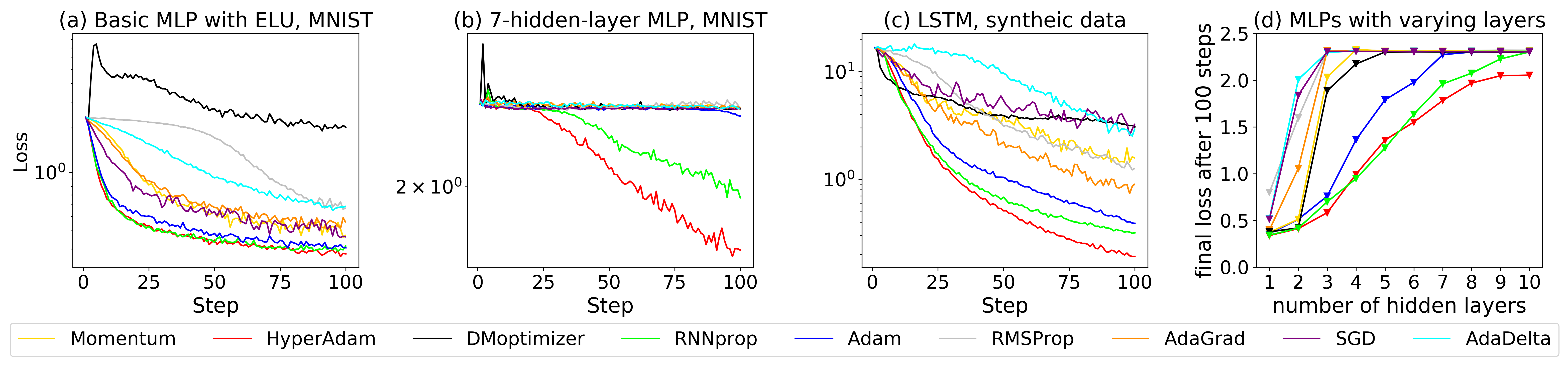
Figure 5: HyperAdam performs best compared with other optimizers on neural networks with different structures.

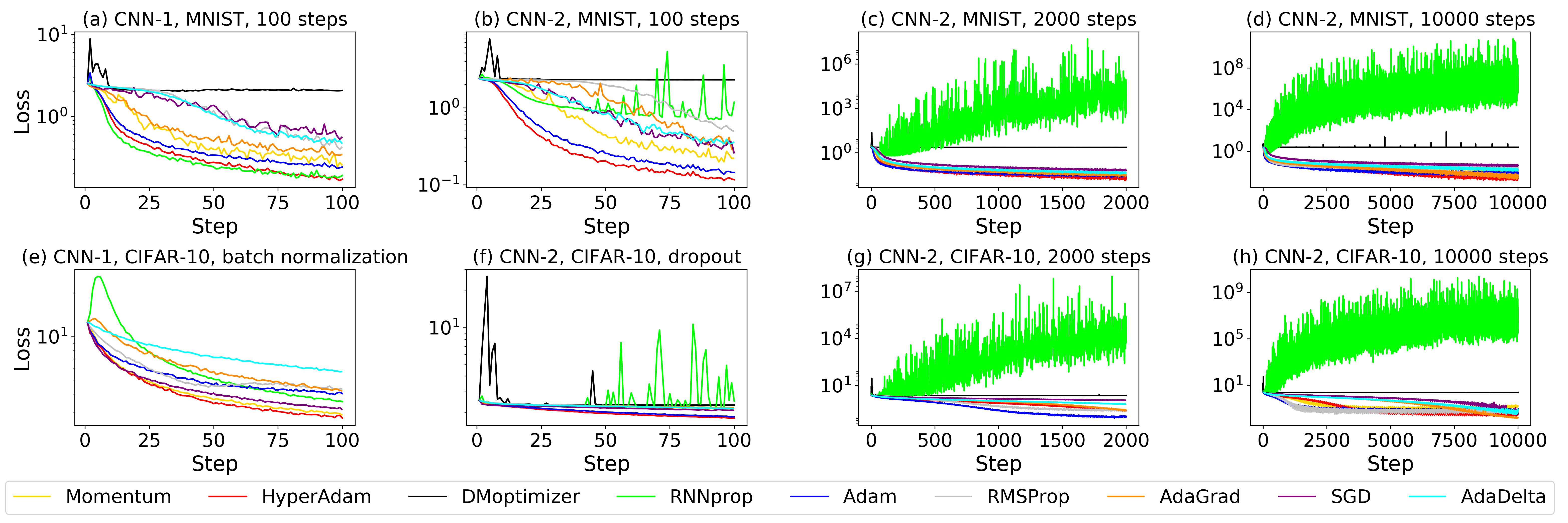
Figure 6: Comparison of different optimizers for optimizing different CNNs in different optimization steps.

5 Evaluation

We have trained HyperAdam based on 1-layer MLP (basic MLP), we now evaluate the learned HyperAdam for more complex networks such as basic MLP with different activation functions, deeper MLP, CNN and LSTM.

• Activation functions: The activation function of basic MLP is extended from sigmoid to ReLU, ELU and tanh.

• Deep MLP: The number of hidden layers of MLP is extended to range of $[2,10]$, and each layer has 20 hidden units and uses sigmoid as activation function.

• CNN: Convolution neural networks are with structures of $c$-$c$-$p$-$f$ (CNN-1) and $c$-$c$-$p$-$c$-$c$-$p$-$f$-$f$ (CNN-2), where $c$, $p$ and $f$ represent convolution, max-pooling and fully-connected layer respectively. Convolution kernel is with size of $3\times 3$ and the max-pooling layer is with size of $2\times 2$ and stride 2. CNN-1 and CNN-2 are also trained with batch normalization and dropout respectively.

• LSTM: LSTM with hidden state in size of 20 is applied to sequence prediction task using mean squared error loss as in (?). Given a sequence $f(0),\dots,f(9)$ with additive noise, the LSTM is supposed to predict the value of $f(10)$. Here $f(x)=A\sin(wx+\phi)$. The dataset is generated with uniformly random sampling $A\sim U(0,10),w\sim U(0,\pi/2),\phi\sim U(0,2\pi)$, and the noise is drawn from Gaussian distribution $N(0,0.1)$.

We also evaluate whether our learned HyperAdam can well generalize to different datasets, e.g. CIFAR-10 (?). Moreover, the HyperAdam is trained assuming it iteratively optimizes network parameters in fixed iterations $T=100$, we also evaluate the learned HyperAdam for longer iterative optimization steps as in (?). The generalization ability of the networks trained by HyperAdam will be also evaluated preliminarily.

In evaluations, we will compare our HyperAdam with traditional network optimizers such as SGD, AdaDelta, Adam, AdaGrad, Momentum, RMSProp, and state-of-the-art learning-based optimizers including RNNprop (?), DMoptimizer (?). For the traditional optimizers, we hand-tuned the learning rates and set other hyperparameters as defaults in TensorFlow. All the initial parameters of learners used in the experiments are sampled independently from the Gaussian distribution. We report the quantitative value as the average measure for training the learner 100 times with random parameter initialization.

5.1 Generalization with Fixed Optimization Steps

We first assume that the learned HyperAdam optimizes the parameters of learners for fixed optimization steps $T=100$, same as the learning procedure for HyperAdam.

Activation	Adam	DMoptimizer	RNNprop	HyperAdam
sigmoid	0.35	0.38	0.34	0.33
ReLU	0.32	1.42	0.31	0.29
ELU	0.31	2.02	0.31	0.28
tanh	0.34	0.83	0.33	0.36

Table 1: Performance for training basic MLP in 100 steps with different activation functions. Each value is the average final loss for optimizing networks in 100 times.

Activation functions

As shown in Table 1, HyperAdam is tested for training basic MLP with different activation functions on MNIST dataset, the loss values in Table 1 show that HyperAdam can best generalize to optimize basic MLP with ReLU, ELU and tanh as activation functions, compared with DMoptimizer and RNNprop. Our HyperAdam also outperforms the basic Adam algorithm. The DMoptimizer can not well generalize to basic MLP with ELU activation function, which can be also visually observed in Fig. 5(a).

Deep MLP

We further evaluate performance of HyperAdam on learning parameters of MLPs with varying layer numbers. According to Fig. 5(d), for different number of hidden layers ranging from 1 to 10, HyperAdam always performs significantly better than Adam and DMoptimizer. Compared with RNNprop, HyperAdam is better in general, especially for deeper MLP with more than 6 layers. The loss curves in Fig. 5(b) of different optimizers for MLP with 7 hidden layers illustrate HyperAdam is significantly better.

LSTM

As shown in Table 2, the “Baseline” task is to utilize one-layer LSTM to predict $f(10)$ on dataset with noise drawn from $N(0,0.1)$, which is further varied by training on dataset with small noise drawn from $N(0,0.01)$ (“Small noise”) or using two-layer LSTM (“2-layer”) for prediction. By comparing the loss values in Table 2, our HyperAdam can better decrease the training losses than the compared optimizers, i.e., Adam, DMoptimizer, RNNprop, HyperAdam. Specifically, Fig. 5(c) shows an example for the comparison in task of “Small noise”.

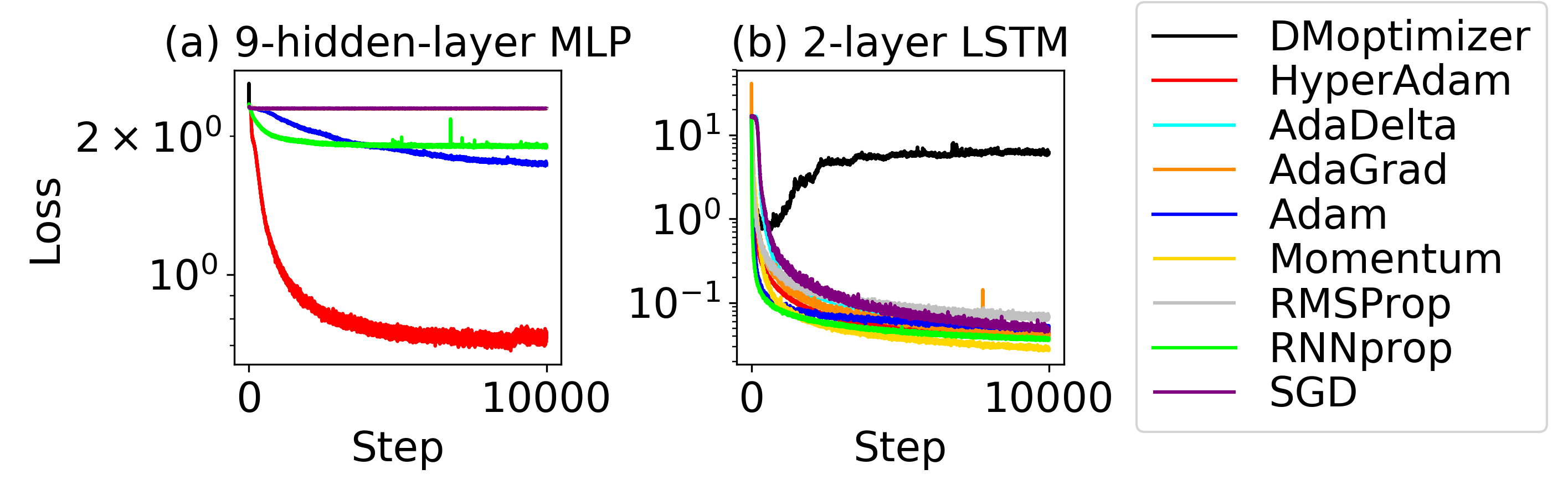
Figure 7: HyperAdam with 10000 optimization steps. Training curves by DMoptimizer, AdaGrad, RMSProp, AdaDelta, Momentum and SGD coincide in the left figure.

Task	Adam	DMoptimizer	RNNprop	HyperAdam
Baseline	0.65	3.10	0.49	0.42
Small noise	0.39	3.06	0.32	0.19
2-layer	0.51	2.05	0.27	0.26

Table 2: Performance on different sequence prediction tasks.

CNN

Figure 6(a)-(b) compare training curves of CNN-1 and CNN-2 on MNIST using different optimizers. Figure 6(e)-(f) compare training curves of CNN-1 with batch normalization and CNN-2 with dropout on CIFAR-10 respectively. In these figures, DMoptimizer and RNNprop do not always perform well or even fail while HyperAdam can effectively decrease the training losses in different tasks.

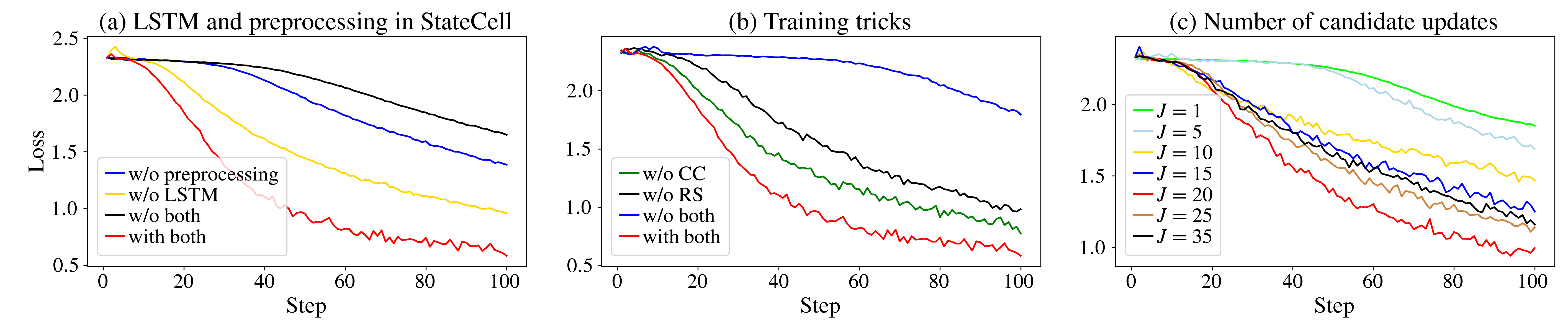
Figure 8: Ablation study for the number of candidate updates, training tricks and structure in StateCell. CC denotes “Combination with Convex function”, and RS denotes “Random Scaling”.

5.2 Generalization to Longer Horizons

We have evaluated HyperAdam for optimizing different learners in fixed optimization steps ($T=100$), same as the meta-training phase. We now evaluate HyperAdam for its effectiveness in running optimization for longer steps.

Deep MLP

Figure 7(a) illustrates the training curves of MLP with 9 hidden layers on MNIST using different optimizers for 10000 steps. DMoptimizer and almost all traditional optimizers, including SGD, Momentum, AdaGrad, AdaDelta and RMSProp, fail to decrease the loss. Our HyperAdam can effectively decrease the training loss.

LSTM

The comparison of training two-layer LSTM to predict $f(10)$ with different optimizers for 10000 steps is shown in Fig. 7(b). DMoptimizer decreases the loss first and then increases the loss dramatically. With similar performance to the traditional optimizers, such as AdaGrad and AdaDelta, our HyperAdam and RNNprop perform better than RMSProp and SGD.

CNN

Figure 6(c)-(d) show the training curves of CNN-2 for 2000 steps and 10000 steps on MNIST dataset. Both RNNprop and DMoptimizer fail to decrease the loss. However, HyperAdam manages to decrease the loss of CNNs and performs slightly better than the traditional network optimizers, such as SGD, Adam and AdaDelta. When training CNN-2 on CIFAR-10 dataset, HyperAdam does not perform as fast as Adam and RMSProp for the first 2000 steps according to Fig. 6(g), but achieves lower loss at 10000th step as shown in Fig. 6(h), while RNNprop and DMoptimizer fail to sufficiently decrease the training loss.

5.3 Generalization of the Learners

The generalization ability of the learners trained by DMoptimizer, RNNprop, Adam and HyperAdam for 10000 steps is evaluated. Table 3 shows the loss, top-1 error and top-2 error of the two learners, CNN-1 and CNN-2 on dataset MNIST, which shows the generalization of learners trained by HyperAdam and Adam are significantly better than those trained by DMoptimizer and RNNprop.

5.4 Ablation Study

We next perform ablation study to justify the effectiveness of key components in HyperAdam.

Task	Measure	Adam	DMoptimizer	RNNprop	HyperAdam
CNN-1 (MNIST)	loss	0.10	2.30	0.36	0.05
	top-1	98.50%	10.10%	96.46%	98.48%
	top-2	99.59%	20.38%	99.03%	99.63%
CNN-2 (MNIST)	loss	0.09	2.30	2.30	0.07
	top-1	98.98%	11.35%	11.37%	99.02%
	top-2	99.80%	21.45%	21.69%	99.78%

Table 3: Generalization of the learner trained by Adam, DMoptimizer, RNNprop and HyperAdam for 10000 steps.

LSTM and preprocessing in StateCell

Figure 8(a) illustrates that HyperAdam achieves lower loss than HyperAdam without LSTM block or (and) preprocessing for training 3-hidden-layer MLP on MNIST, which reflects that the LSTM block and preprocessing help strengthen HyperAdam.

Training tricks

We justify the effectiveness of “Random Sampling” and “Combination with Convex Functions” in our proposed HyperAdam. As shown in Fig. 8(b), HyperAdam trained with both two tricks performs better than HyperAdam trained with either one of them and neither of them for training loss of 3-hidden-layer MLP on MNIST as optimizee, which indicates that the two tricks can enhance the generalization ability of learned HyperAdam.

Number of candidate updates

Figure 8(c) shows the comparison for optimizing cross entropy loss of 4-hidden-layer MLP on MNIST dataset with HyperAdam having different number of candidate updates ($J=1,5,10,15,20,25,35$). It is observed that the performance of HyperAdam is improved first with the increase of $J$ until 20 achieving best performance, then becomes saturated and decreased with larger number of candidate updates. But all the HyperAdams with $J=5,10,15,25,35$ are better than the baseline with single candidate update.

5.5 Computation Time

The time consuming for computing each update by HyperAdam is roughly the same with that of DMoptimizer and RNNprop. For example, the time consuming for computing each update given gradient of a 9-hidden-layer MLP is 0.0023s, 0.0033s and 0.0039s for DMoptimizer, HyperAdam and RNNprop respectively in average. Though faster for computing each update than HyperAdam, Adam is not as efficient as HyperAdam to sufficiently decrease the training loss. When training 8-hidden-layer MLP for 10000 steps, HyperAdam takes 26.33s to decrease the loss to 0.64 (the lowest loss that Adam can achieve) while Adam takes 28.97s to decrease loss to 0.64 and finally achieves loss of 0.52.

6 Conclusion and Future Work

In this paper, we proposed a novel optimizer HyperAdam implementing “learning to optimize” inspired by the traditional Adam optimizer and ensemble learning. It adaptively combines the multiple candidate parameter updates generated by Adam with multiple adaptively learned decay rates. Based on this motivation, a carefully designed RNN was proposed for implementing HyperAdam optimizer. It was justified to outperform or match traditional optimizers such as Adam, SGD and state-of-art learning-based optimizers in diverse networks training tasks.

In the future, we are interested in applying HyperAdam to train larger scale and more complex networks in vision, NLP, etc., and modeling the correlations among parameter coordinates to further enhance its performance.

7 Acknowledgment

This research was supported by the National Natural Science Foundation of China under Grant Nos. 11622106, 11690011, 61721002, 61472313.

8 Supplementation

In this supplementary material, we will prove lemma 1 and the claim that HyperAdam is invariant to the scale of gradient (scale invariance) in the submitted paper.

We first present the proof of lemma 1 in Section 3.2.

Lemma.

$\hat{\beta}_{t}=\beta\hat{\beta}_{t-1}+(1-\beta)$ with $\hat{\beta}_{0}=0$ is the online formula of $\hat{\beta}_{t}=1-\beta^{t}$.

Proof.

Since $\hat{\beta}_{0}=0$, we derive that:

$$\hat{\beta}_{t} =\beta\hat{\beta}_{t-1}+(1-\beta)$$

$$=\beta(\beta\hat{\beta}_{t-2}+(1-\beta))+(1-\beta)$$

$$=\cdots$$

$$=\beta^{t}\hat{\beta}_{0}+(1-\beta)\Sigma_{i=1}^{t}\beta^{t-i}$$

$$=1-\beta^{t},$$

so the lemma is proved. $\blacksquare$

We then prove the claim on scale invariance described in Section 3.2.

Claim.

Same to Adam, HyperAdam is also invariant to the scale of gradient when ignoring $\varepsilon$.

Proof.

In order to prove the claim, we only need to verify that $\mathbf{s}_{t},\bm{\beta}_{t},\bm{\gamma}_{t}$ and $\bm{\rho}_{t}$ are invariant to the scale of gradient.

Since the gradient will be normalized when it acts as input of the state function $F_{h}$ corresponding to StateCell, we can rewrite $F_{h}$ as

$$\mathbf{s}_{t}=F_{h}(\mathbf{s}_{t-1},g_{t};\varTheta_{h})\triangleq F^{\prime}_{h}(\mathbf{s}_{t-1},\frac{g_{t}}{\lVert g_{t}\rVert};\varTheta_{h}).$$ (10)

We next consider the scaled gradient $sg_{t}$:

$$F_{h}(\mathbf{s}_{t-1},sg_{t};\varTheta_{h}) =F^{\prime}_{h}(\mathbf{s}_{t-1},\frac{sg_{t}}{\lVert sg_{t}\rVert};\varTheta_{h})$$

$$=F^{\prime}_{h}(\mathbf{s}_{t-1},\frac{g_{t}}{\lVert g_{t}\rVert};\varTheta_{h})$$

$$=F_{h}(\mathbf{s}_{t-1},g_{t};\varTheta_{h}).$$

so $\mathbf{s}_{t}$ outputted by StateCell is invariant to the scale of the gradient. We can similarly derive that $\bm{\rho}_{t}=F_{q}(\mathbf{s}_{t};\varTheta_{q})$, corresponding to the WeightCell, is invariant to the scale of gradient. Furthermore, the fact that $\bm{\beta}_{t},\bm{\gamma}_{t}$ are invariant to the scale of gradient can also be proved in the same way.

Since decay rates $\bm{\beta}_{t},\bm{\gamma}_{t}$ are scale invariant, candidate updates $\hat{m}_{t}^{j}$ ($j=1,\dots,J$) outputted by AdamCell are invariant to the scale of gradient. Therefore, the final update $d_{t}=\Sigma_{j=1}^{J}\rho_{t}^{j}\odot\hat{m}_{t}^{j}$ is invariant to the scale of gradient. $\blacksquare$

References

- [Amit and Meir 2018] Amit, R., and Meir, R. 2018. Meta-learning by adjusting priors based on extended PAC-Bayes theory. In ICML, 205–214.
- [Andrychowicz et al. 2016] Andrychowicz, M.; Denil, M.; Gomez, S.; Hoffman, M. W.; Pfau, D.; Schaul, T.; Shillingford, B.; and De Freitas, N. 2016. Learning to learn by gradient descent by gradient descent. In NIPS, 3981–3989.
- [Chen et al. 2017] Chen, Y.; Hoffman, M. W.; Colmenarejo, S. G.; Denil, M.; Lillicrap, T. P.; Botvinick, M.; and Freitas, N. 2017. Learning to learn without gradient descent by gradient descent. In ICML, 748–756.
- [Clevert and and 2016] Clevert, D., and and, T. U. 2016. Fast and accurate deep network learning by exponential linear units (elus). In ICLR.
- [Daniel, Taylor, and Nowozin 2016] Daniel, C.; Taylor, J.; and Nowozin, S. 2016. Learning step size controllers for robust neural network training. In AAAI, 1519–1525.
- [Dauphin et al. 2014] Dauphin, Y. N.; Pascanu, R.; Gulcehre, C.; Cho, K.; Ganguli, S.; and Bengio, Y. 2014. Identifying and attacking the saddle point problem in high-dimensional non-convex optimization. In NIPS, 2933–2941.
- [Duchi, Hazan, and Singer 2011] Duchi, J.; Hazan, E.; and Singer, Y. 2011. Adaptive subgradient methods for online learning and stochastic optimization. Journal of Machine Learning Research 12:2121–2159.
- [Finn et al. 2017] Finn, C.; Yu, T.; Zhang, T.; Abbeel, P.; and Levine, S. 2017. One-shot visual imitation learning via meta-learning. In CoRL, 357–368.
- [Goodfellow et al. 2014] Goodfellow, I.; Pouget-Abadie, J.; Mirza, M.; Xu, B.; Warde-Farley, D.; Ozair, S.; Courville, A.; and Bengio, Y. 2014. Generative adversarial nets. In NIPS, 2672–2680.
- [He et al. 2016] He, K.; Zhang, X.; Ren, S.; and Sun, J. 2016. Deep residual learning for image recognition. In CVPR, 770–778.
- [Hochreiter, Younger, and Conwell 2001] Hochreiter, S.; Younger, A. S.; and Conwell, P. R. 2001. Learning to learn using gradient descent. In ICANN, 87–94.
- [Kingma and Ba 2015] Kingma, D. P., and Ba, J. 2015. Adam: A method for stochastic optimization. In ICLR.
- [Krizhevsky 2009] Krizhevsky, A. 2009. Learning multiple layers of features from tiny images. Technical report.
- [LeCun, Bengio, and Hinton 2015] LeCun, Y.; Bengio, Y.; and Hinton, G. 2015. Deep learning. Nature 521(7553):436.
- [LeCun et al. 1998] LeCun, Y.; Bottou, L.; Bengio, Y.; and Haffner, P. 1998. Gradient-based learning applied to document recognition. Proceedings of the IEEE 86(11):2278–2324.
- [Li and Malik 2016] Li, K., and Malik, J. 2016. Learning to optimize. In ICLR.
- [Lillicrap et al. 2016] Lillicrap, T. P.; Hunt, J. J.; Pritzel, A.; Heess, N.; Erez, T.; Tassa, Y.; Silver, D.; and Wierstra, D. 2016. Continuous control with deep reinforcement learning. In ICLR.
- [Liu et al. 2018] Liu, R.; Fan, X.; Cheng, S.; Wang, X.; and Luo, Z. 2018. Proximal alternating direction network: A globally converged deep unrolling framework. In AAAI, 1371–1378.
- [Lv, Jiang, and Li 2017] Lv, K.; Jiang, S.; and Li, J. 2017. Learning gradient descent: Better generalization and longer horizons. In ICML, 2247–2255.
- [Marino, Yue, and Mandt 2018] Marino, J.; Yue, Y.; and Mandt, S. 2018. Learning to infer. In ICLR.
- [McMahan and Rao 2018] McMahan, B., and Rao, D. 2018. Listening to the world improves speech command recognition. In AAAI, 378–385.
- [Naik and Mammone 1992] Naik, D. K., and Mammone, R. 1992. Meta-neural networks that learn by learning. In IJCNN, 437–442.
- [Reddi, Kale, and Kumar 2018] Reddi, S. J.; Kale, S.; and Kumar, S. 2018. On the convergence of adam and beyond. In ICLR.
- [Reiter and Schmidhuber 1997] Reiter, S., and Schmidhuber, J. 1997. Long short-term memory. Neural Computation 9:1735–80.
- [Ren et al. 2018] Ren, M.; Ravi, S.; Triantafillou, E.; Snell, J.; Swersky, K.; Tenenbaum, J. B.; Larochelle, H.; and Zemel, R. S. 2018. Meta-learning for semi-supervised few-shot classification. In ICLR.
- [Robbins and Monro 1951] Robbins, H., and Monro, S. 1951. A stochastic approximation method. The Annals of Mathematical Statistics 22(3):400–407.
- [Santoro et al. 2016] Santoro, A.; Bartunov, S.; Botvinick, M.; Wierstra, D.; and Lillicrap, T. 2016. Meta-learning with memory-augmented neural networks. In ICML, 1842–1850.
- [Schmidhuber 1992] Schmidhuber, J. 1992. Learning to control fast-weight memories: An alternative to dynamic recurrent networks. Neural Computation 4(1):131–139.
- [Snell, Swersky, and Zemel 2017] Snell, J.; Swersky, K.; and Zemel, R. 2017. Prototypical networks for few-shot learning. In NIPS, 4077–4087.
- [Sutskever, Vinyals, and Le 2014] Sutskever, I.; Vinyals, O.; and Le, Q. V. 2014. Sequence to sequence learning with neural networks. In NIPS, 3104–3112.
- [Tieleman and Hinton 2012] Tieleman, T., and Hinton, G. 2012. Lecture 6.5-rmsprop: Divide the gradient by a running average of its recent magnitude. COURSERA: Neural Networks for Machine Learning 4(2):26–31.
- [Tseng 1998] Tseng, P. 1998. An incremental gradient (-projection) method with momentum term and adaptive stepsize rule. SIAM Journal on Optimization 8(2):506–531.
- [Werbos 1990] Werbos, P. 1990. Backpropagation through time: what it does and how to do it. Proceedings of the IEEE 78:1550 – 1560.
- [Wichrowska et al. 2017] Wichrowska, O.; Maheswaranathan, N.; Hoffman, M. W.; Colmenarejo, S. G.; Denil, M.; de Freitas, N.; and Sohl-Dickstein, J. 2017. Learned optimizers that scale and generalize. In ICML, 3751–3760.
- [Wolpert 1992] Wolpert, D. H. 1992. Stacked generalization. Neural Networks 5(2):241–259.
- [Yang et al. 2016] Yang, Y.; Sun, J.; Li, H.; and Xu, Z. 2016. Deep admm-net for compressive sensing mri. In NIPS, 10–18.
- [Younger, Hochreiter, and Conwell 2001] Younger, A. S.; Hochreiter, S.; and Conwell, P. R. 2001. Meta-learning with backpropagation. In IJCNN, 2001–2006.
- [Zeiler 2012] Zeiler, M. D. 2012. Adadelta: an adaptive learning rate method. arXiv preprint arXiv:1212.5701.