Two-fluid theory for superfluid system with anisotropic effective masses

Abstract

In this work, we generalize the two-fluid theory to a superfluid system with anisotropic effective masses along different principal axis directions. As a specific example, such a theory can be applied to spin-orbit coupled Bose-Einstein condensate (BEC) at low temperature. The normal density from phonon excitations and the second sound velocity are obtained analytically. Near the phase transition from the plane wave to zero-momentum phases, due to the effective mass divergence, the normal density from phonon excitation increases greatly, while the second sound velocity is suppressed significantly. With quantum hydrodynamic formalism, we give a unified derivation for suppressed superfluid density and Josephson relation. At last, the momentum distribution function and fluctuation of phase for the long wave length are also discussed.

I Introduction

At low temperature, Bose-Einstein condensation and superfluidity would occur in bosonic system. Tissa Tisza and Landau Landau propose two-fluid theory to explain the superfluid phenomena in Helium-4. Comparing with usual classical fluid, due to an extra degree of freedom (existence of condensate), the existence of second sound is an important characteristic of superfluidity. With realizations of Bose-Einstein condensate (BEC) and fermion superfluidity in dilute atomic gas, the second sound and other related superfluid phenomena in atomic gas have attracted great interests Taylor2005 ; He2007 ; Taylor2009 ; Hu2014 ; Hou2013 ; Meppelink2009 ; Tey2013 . For example, sound velocities at zero temperature as a function of density in cold atoms Andrews1997 ; Joseph2007 have been measured experimentally. The application of two-fluid theory for sound propagations in cold atomic gas has been proposed Zaremba1998 ; Shenoy1998 . The predictions on the second sound Heiselberg2006 ; Arahata2009 and the quenched moment of inertia Baym2013 resulting from superfluidity in cold atoms has been observed experimentally Riedl2011 ; Sidorenkov2013 . According to the two-fluid theory, the whole fluid can be viewed as a mixture of two component fluids, namely, the normal part and superfluid part. The motions of normal part result in viscosity, while the motions of superfluid one are dissipationless. As temperature grows from absolute zero to superfluid transition point, the superfluid density decreases from total density to zero. Specially, the normal density at usual superfluid system (Helium-4 fluid or cold atoms) is vanishing at zero temperature. Consequently, the moment of inertia is also vanishing in usual isotropic superfluid system at zero temperature.

Recently spin-orbit coupled BEC has been realized experimentally Lin1 ; Wang2 ; Cheuk ; zhangjinyi ; Olson ; Khamehchi . There exist a phase transition between the plane wave phase and the zero momentum phase in the spin-orbit coupled BEC Lin1 ; zhangshizhong . It is shown that, even at zero temperature, there exists finite normal density, and even all the total density becomes normal at the phase transition point although the condensate fraction is finite normaldensity . At zero temperature, due to finite normal density, there is finite momentum of inertia in the spin-orbit coupled BEC stringari2016 . It is shown that the suppressing of superfluid density is closely related to enhancements of effective masses near the ground state. Because the effective masses enhance anisotropically, the expansion behaviors of spin-orbit coupled gas also shows anisotropy Martone2012 ; Qu2017 ; zhangyongping .

It is expected that due to enhancements of effective masses in spin-orbit coupled BEC, the corresponding two-fluid theory at finite temperature also need to be revised greatly. In this work, we generalize the two-fluid theory to a superfluid system with anisotropic effective masses along different principal axis directions. As an immediate application, we find that a lot of superfluid properties of spin-orbit coupled BEC, e.g., the decreasing of superfluid density, the suppressed anisotropic sound velocities, etc., can be described by an anisotropic two-fluid theory. Near the phase transition from the plane wave to zero-momentum phases, the normal density from phonon excitation increases greatly, while the second sound velocity is suppressed significantly.

The paper is organized as follows. In Sec. II, we review the thermodynamic relations for superfluid system. In Sec. III, based on the entropy equation, we give a derivation for dissipationless two-fluid equations. In Sec. IV, as an application of the anisotropic two-fluid theory, we give a specific example, namely, spin-orbit coupled BEC, to illustrate the above results. A summary is given in Sec. V.

II Thermodynamic relations for superfluid system

First of all, we consider an original system $K_{0}$ with the particle mass $m$, in which the many-particle Hamiltonian

$$H_{0}=\sum_{i}\frac{\mathbf{p}_{0i}^{2}}{2m}+\frac{1}{2}\sum_{i\neq j}V(\mathbf{r}_{i}-\mathbf{r}_{j}),$$ (1)

where $\mathbf{p}_{0i}$ is the particle momentum for $K_{0}$ and $V(\mathbf{r}_{i}-\mathbf{r}_{j})$ is the interaction potential between particles $i$ and $j$. In the following, we mainly investigate the effects arising from enhancements of the effective masses, i.e., $m\rightarrow zm$ with $z>1$. For this purpose, we consider another system $K$ with the effective mass $m^{\prime}=zm$. The corresponding Hamiltonian and Lagrangian are written as

$$H=\sum_{i}\frac{\mathbf{p}_{i}^{2}}{2zm}+\frac{1}{2}\sum_{i\neq j}V(\mathbf{r}_{i}-\mathbf{r}_{j}),$$

$$L=\sum_{i}\frac{zm\mathbf{\tilde{v}}_{i}^{2}}{2}-\frac{1}{2}\sum_{i\neq j}V(\mathbf{r}_{i}-\mathbf{r}_{j}),$$

where $\mathbf{p}_{i}$ and $\mathbf{\tilde{v}}_{i}$ are the particle momentum and velocity for $K$, respectively. From the Hamilton’s canonical equations (or the Newton’s second law), i.e., $d\mathbf{p}_{0i}/dt=-\partial V/\partial\mathbf{r}_{i}$ and $d\mathbf{p}_{i}/dt=-\partial V/\partial\mathbf{r}_{i}$, and the relations $\mathbf{p}_{0i}=m\mathbf{v}_{0i}$, $\mathbf{p}_{i}=zm\mathbf{\tilde{v}}_{i}$, we get the velocity for $K$ in terms of that of $K_{0}$, i.e.,

$$\mathbf{\tilde{v}_{i}}=\mathbf{v}_{0i}/z,$$ (2)

where $\mathbf{v}_{0i}$ is the particle velocity for $K_{0}$ with the mass $m$. Equation (2) shows that the enhancements of masses would result in the decreasing of velocity. In the following, the velocity appearing in expressions is always referred to that of the original system $K_{0}$, which has the mass $m$, rather $zm$. The Lagrangian for $K$ can also be expressed in terms of $\mathbf{v}_{0i}$, i.e.,

$$L=\sum_{i}\frac{m\mathbf{v}_{0i}^{2}}{2z}-\frac{1}{2}\sum_{i\neq j}V(\mathbf{r}_{i}-\mathbf{r}_{j}).$$

In order to get the thermodynamic relations, now we consider a moving reference frame with the velocity $\mathbf{u}$ with respect to the laboratory reference frame. The particle velocity in the moving frame is

$$\mathbf{v}^{\prime}_{i}=\mathbf{v}_{0i}-\mathbf{u}.$$ (3)

The Lagrangian $L$ is rewritten as

$$L=\sum_{i}\frac{m(\mathbf{v}{{}^{\prime}}_{i}+\mathbf{u})^{2}}{2z}-\frac{1}{2}\sum_{i\neq j}V(\mathbf{r}_{i}-\mathbf{r}_{j}).$$

The canonical momentum and Hamiltonian in the moving frame are thus given respectively by

$$\mathbf{p}^{\prime}_{i}\equiv\frac{\partial L}{\partial\mathbf{v}^{\prime}}_{i}=m(\mathbf{v}^{\prime}_{i}+\mathbf{u})/z=\mathbf{p}_{0i}/z=\mathbf{p}_{i}/z.$$

$$H^{\prime}\equiv\sum_{i}\mathbf{p}_{i}^{\prime}\cdot\mathbf{v}_{i}^{\prime}-L=H-\frac{\mathbf{u}}{z}\cdot\mathbf{P},$$

where the total momentum $\mathbf{P}=\sum_{i}\mathbf{p}_{i}$.

In terms of the Hamiltonian $H^{\prime}$, the partition function

$$Z\equiv tre^{-\beta H^{\prime}}=e^{-\beta F}=e^{-\beta[E-TS-\mathbf{u}\cdot\mathbf{P}/z]},$$ (4)

where $E$ is the energy in the laboratory frame, $S$ is the entropy, $\beta=1/T$ is the inverse temperature, and the free energy

$$F=E-TS-\mathbf{u}\cdot\mathbf{P}/z.$$ (5)

The grand potential

$$\Omega\equiv-pV=F-\mu N=E-TS-\mathbf{u}\cdot\mathbf{P}/z-\mu N,$$

where $p$ is the pressure, $V$ is the system volume, $\mu$ is the chemical potential, and $N$ is the total particle number. Further introducing the energy density $\epsilon=E/V$, the entropy density $s=S/V$, the momentum density $\mathbf{g}=\mathbf{P}/V$, and the particle number density $n=N/V$, the pressure is given by

$$p=-\epsilon+Ts+\mathbf{u}\cdot\mathbf{g}/z+\mu n.$$ (6)

Since the free energy is a function of $\left\{T,V,\mathbf{u},N\right\}$, e.g., $F=F(T,V,\mathbf{u},N)$, using Eq. (5), we obtain

$$dF=-SdT-pdV+\mu dN-\mathbf{P}\cdot d\mathbf{u}/z$$

$$=dE-TdS-SdT-\mathbf{u}\cdot d\mathbf{P}/z-\mathbf{P}\cdot d\mathbf{u}/z,$$ (7)

which leads to the fundamental thermodynamic relation

$$TdS=dE+pdV-\mu dN-\mathbf{u}\cdot d\mathbf{P}/z.$$ (8)

For a fixed unit volume ($dV\equiv 0$), Eq. (8) turns into

$$Tds=d\epsilon-\mu dn-m\mathbf{u}\cdot d\mathbf{j},$$ (9)

where $\mathbf{j}\equiv\mathbf{g}/(zm)$ is the particle current density.

On the other hand, using $\mathbf{p}_{i}^{2}/(2zm)-\mathbf{u}\cdot\mathbf{p}_{i}/z=(\mathbf{p}_{i}-m\mathbf{u})^{2}/(2zm)-m\mathbf{u}^{2}/(2z)$, Eq. (4) becomes

$$Z=e^{\beta Nm\mathbf{u}^{2}/(2z)}Z_{0}\equiv e^{\beta Nm\mathbf{u}^{2}/(2z)}tre^{-\beta H},$$

where $Z_{0}=tre^{-\beta H}\equiv e^{-\beta F_{0}}$ and $F_{0}$ is the free energy when the fluid is at rest. So the free energy

$$F=F_{0}-Nm\mathbf{u}^{2}/(2z).$$ (10)

For superfluid system, Eq. (10) can be extended to a case in which the superfluid and normal parts move with the velocities $\mathbf{v}_{s}=\hbar\mathbf{\nabla}\theta/m$ and $\mathbf{v}_{n}=\mathbf{u}$, respectively Chaikin , where $\theta$ is the phase of the condensate order parameter. In this case, the free energy density, $f=F/V$, is given by

$$f=f_{0}-nm\mathbf{v}_{n}^{2}/(2z)+n_{s}m(\mathbf{v}_{s}-\mathbf{v}_{n})^{2}/(2z),$$ (11)

where $f_{0}$ is the free energy density when the fluid is at rest. The term $n_{s}m(\mathbf{v}_{s}-\mathbf{v}_{n})^{2}/(2z)$ describes an extra energy due to the motion of the superfluid part relative to the normal part, and $n_{s}$ is the particle number density of the superfluid part. We should remind that the velocity for $K$ is $\mathbf{\tilde{v}}_{s(n)}=\mathbf{v}_{s(n)}/z$.

The free energy density $f$ is a function of independent variables $\{T,n,\mathbf{v}_{n},\mathbf{v}_{s}\}$. Similarly as Eq. (II), its variation can be written as

$$df=-sdT+\mu dn-m\mathbf{j}\cdot d\mathbf{v}_{n}+\mathbf{h}\cdot d\mathbf{v}_{s},$$ (12)

where $\mathbf{h}\equiv\partial f/\partial\mathbf{v}_{s}$ is the thermodynamic conjugate variable of $\mathbf{{v}_{s}}$. From Eqs. (11) and (12), the particle current density and the conjugate variable of $\mathbf{v}_{s}$ are given respectively by

$$\mathbf{j}=-\frac{\partial f}{m\partial\mathbf{v}_{n}}=\frac{n_{n}\mathbf{v}_{n}+n_{s}\mathbf{v}_{s}}{z},$$

$$\mathbf{h}=\frac{\partial f}{\partial\mathbf{v}_{s}}=\frac{n_{s}m(\mathbf{v}_{s}-\mathbf{v}_{n})}{z},$$ (13)

where $n_{n}\equiv n-n_{s}$ is the particle number density of the normal part. From Eqs. (II) and (II), the thermodynamic relations are generalized as

$$p=-\epsilon+Ts+m\mathbf{v}_{n}\cdot\mathbf{j}+\mu n,$$

$$Tds=d\epsilon-\mu dn-m\mathbf{v}_{n}\cdot d\mathbf{j}-\mathbf{h}\cdot d\mathbf{v}_{s},$$

$$dp=sdT+nd\mu+m\mathbf{j}\cdot d\mathbf{v}_{n}-\mathbf{h}\cdot d\mathbf{v}_{s}.$$ (14)

Equation (II) also holds for the anisotropic superfluid system.

III two-fluid equations for anisotropic effective masses

Having obtained the fundamental thermodynamic relations in Eqs. (II) and (II), in this section we extend them to derive the required two-fluid equations for anisotropic effective masses. For an anisotropic system with different effective masses along three principal axis directions, the Hamiltonian

$$H=H_{0}+H_{\text{int}},$$

$$H_{0}=\int d^{3}\mathbf{r}\psi^{\dagger}\left(\frac{p_{x}^{2}}{2m_{1}}+\frac{p_{y}^{2}}{2m_{2}}+\frac{p_{z}^{2}}{2m_{3}}\right)\psi,$$

$$H_{\text{int}}=\frac{1}{2}\int d^{3}\mathbf{r}_{1}d^{3}\mathbf{r}_{2}\psi^{\dagger}(\mathbf{r}_{1})\psi^{\dagger}(\mathbf{r}_{2})V(\mathbf{r}_{1}-\mathbf{r}_{2})\psi(\mathbf{r}_{2})\psi(\mathbf{r}_{1}),$$ (15)

where $m_{i}$ is the effective mass along the $i$th axis and $\psi$ is the bosonic field operator. We should note that although the masses are anisotropic, the Hamiltonian (15) still has Galilean transformation invariance Hou2015 , and can describe the spin-orbit coupled BEC near the ground state realized in recent experiments Lin1 . In specific, we write the effective mass as

$$m_{i}=mz_{i},$$

where $z_{i=1,2,3}\geq 1$ characterize the enhancements of masses.

III.1 Two-fluid equations

To obtain the two-fluid equations for the Hamiltonian (15), we generalize the free energy density in Eq. (11) as

$$f=f_{0}(T,n)-\sum_{i=1,2,3}\frac{nmv_{ni}^{2}}{2z_{i}}+\sum_{i=1,2,3}\frac{n_{s}m(v_{si}-v_{ni})^{2}}{2z_{i}}.$$ (16)

Based on Eqs. (II) and (16), the particle current density and the conjugate variable of the superfluid velocity of the $i$th axis are given respectively by

$$j_{i}=-\frac{\partial f}{m\partial v_{ni}}=\frac{n_{n}v_{ni}+n_{s}v_{si}}{z_{i}},$$

$$h_{i}=\frac{\partial f}{\partial v_{si}}=\frac{n_{s}m(v_{si}-v_{ni})}{z_{i}}.$$ (17)

Although there exists anisotropy, the particle number, momentum and energy are still conserved. The corresponding continuity equations are given respectively by

$$\frac{\partial n}{\partial t}+\sum_{i}\partial_{i}j_{i}=0,$$ (18)

$$\frac{\partial g_{i}}{\partial t}+\sum_{j}\partial_{j}\pi_{ij}=0,$$ (19)

$$\frac{\partial\epsilon}{\partial t}+\sum_{i}\partial_{i}j_{i}^{\epsilon}=0,$$ (20)

where $g_{i}=m_{i}j_{i}=z_{i}mj_{i}$, $\pi_{ij}$ is the pressure tensor and $j_{i}^{\epsilon}$ is the energy current density. The superfluid velocity can be written as a gradient of condensate phase, i.e., $\mathbf{v}_{s}=\hbar\mathbf{\nabla}\theta/m$. Therefore, the superfluid velocity $\mathbf{v}_{s}$ is irrotational and satisfies the equation fluid

$$\frac{m\partial v_{si}}{\partial t}+\partial_{i}(\mu+X)=0,$$ (21)

where $\mu$ is the chemical potential and $X$ is a scalar function which need to be determined by an entropy equation (see the following). The irrotationality condition is

$$\partial_{i}v_{sj}=\partial_{j}v_{si}.$$ (22)

We should note that the superfluid velocity for the anisotropic system with the mass $z_{i}m$, i.e., $\tilde{v}_{si}=v_{si}/z_{i}$ [see Eq. (2)] would have no irrotationality stringari2016 due to $z_{i}\neq z_{j}$ in general.

The entropy equation can be derived as follows. Using the thermodynamic relations in Eq. (II), continuity equations (18)-(20), Eqs. (21) and (22), we get

$$T\left[\frac{\partial s}{\partial t}+\sum_{i}\partial_{i}\left(\frac{sv_{ni}}{z_{i}}+\frac{Q_{i}}{T}\right)\right]$$

$$=-\sum_{i}Q_{i}\frac{\partial_{i}T}{T}$$

$$-\sum_{i}\left(\frac{g_{i}}{z_{i}m}-\frac{nv_{ni}}{z_{i}}-\frac{h_{i}}{m}\right)\partial_{i}\mu$$

$$-\sum_{ij}\left(\frac{\pi_{ji}}{z_{j}}-\frac{p}{z_{i}}\delta_{ij}-\frac{mj_{j}v_{ni}}{z_{i}}-\frac{v_{sj}h_{i}}{z_{j}}\right)\partial_{i}v_{nj}$$

$$-\sum_{i}\left(\frac{X}{m}-\sum_{j}\frac{v_{sj}v_{nj}}{z_{j}}\right)\partial_{i}h_{i}.$$ (23)

In deriving Eq. (III.1), we have introduced the heat current density $\mathbf{Q}$ with

$$Q_{i}\equiv j_{i}^{\epsilon}-\frac{\mu(g_{i}/m-nv_{ni})}{z_{i}}-\sum_{j}\frac{v_{nj}\pi_{ji}}{z_{j}}-\frac{\epsilon v_{ni}}{z_{i}}$$

$$+\sum_{j}\frac{mv_{ni}v_{nj}j_{j}}{z_{i}}+\left(\sum_{j}\frac{v_{nj}v_{sj}}{z_{j}}-\frac{X}{m}\right)h_{i},$$

and used the thermodynamic relation $p=-\epsilon+Ts+m\mathbf{v}_{n}\mathbf{j}+\mu n$. The right-hand side of Eq. (III.1) is a form of “currents” time “forces” for entropy production. For dissipationless process, the entropy production should be zero, so the right-hand side should vanish, i.e.,

$$Q_{i}=0,$$

$$\frac{g_{i}}{z_{i}m}-\frac{nv_{ni}}{z_{i}}-\frac{h_{i}}{m}=0,$$

$$\frac{\pi_{ji}}{z_{j}}-\frac{p\delta_{ij}}{z_{i}}-\frac{mj_{j}v_{ni}}{z_{i}}-\frac{v_{sj}h_{i}}{z_{j}}=0,$$

$$\frac{X}{m}-\sum_{j}\frac{v_{sj}v_{nj}}{z_{j}}=0.$$ (24)

From Eq. (III.1), we get constitutive relations

$$X=\sum_{j}\frac{mv_{sj}v_{nj}}{z_{j}},$$

$$g_{i}=mnv_{ni}+z_{i}h_{i}=n_{n}mv_{ni}+n_{s}mv_{si}=z_{i}mj_{i},$$

$$\pi_{ji}=p\delta_{ij}+\frac{z_{j}mj_{j}v_{ni}}{z_{i}}+v_{sj}h_{i},$$

$$j_{i}^{\epsilon}=\frac{\mu(g_{i}/m-nv_{ni})}{z_{i}}+\frac{v_{nj}\pi_{ji}}{z_{j}}+\frac{\epsilon v_{ni}}{z_{i}}-\frac{mv_{ni}v_{nj}j_{j}}{z_{i}}.$$ (25)

Due to Eq. (III.1), the entropy equation (III.1) becomes its conservation equation

$$\frac{\partial s}{\partial t}+\sum_{i}\partial_{i}\left(\frac{sv_{ni}}{z_{i}}\right)=0.$$ (26)

The energy conservation equation can be replaced by the entropy conservation equation. Finally, we have four complete equations for the two-fluid theory

$$\frac{\partial n}{\partial t}+\sum_{i}\partial_{i}j_{i}=0,$$ (27)

$$\frac{\partial g_{i}}{\partial t}+\sum_{j}\partial_{j}\pi_{ij}=0,$$ (28)

$$\frac{\partial s}{\partial t}+\sum_{i}\partial_{i}\left(\frac{sv_{ni}}{z_{i}}\right)=0,$$ (29)

$$\frac{m\partial v_{si}}{\partial t}+\partial_{i}\left(\mu+\sum_{j}\frac{mv_{sj}v_{nj}}{z_{j}}\right)=0,$$ (30)

with constitutive relations

$$j_{i}=\frac{n_{n}v_{ni}+n_{s}v_{si}}{z_{i}},$$

$$g_{i}=z_{i}mj_{i}=mn_{n}v_{ni}+mn_{s}v_{si},$$

$$\pi_{ji}=p\delta_{ij}+\frac{mn_{n}v_{nj}v_{ni}+mn_{s}v_{sj}v_{si}}{z_{i}}.$$

Equations (27)-(30) are the main results of this paper. These equations have several important properties. Firstly, due to $z_{i}\neq z_{j}$ in general, the pressure tensor $\pi_{ij}$ would not be a symmetrical tensor in the anisotropic case, i.e., $\pi_{ij}\neq\pi_{ji}$.

Secondly, when $z_{1}=z_{2}=z_{3}=1$, using the relation between the energy ($\epsilon$) of the laboratory frame and that ($\epsilon_{0}$) of another reference frame where the superfluid part is at rest fluid , i.e., $\epsilon=nm\mathbf{v}_{s}^{2}/2+\mathbf{g}_{0}\cdot\mathbf{v}_{s}+\epsilon_{0}$ with $\mathbf{g}_{0}=n_{n}m(\mathbf{v}_{n}-\mathbf{v}_{s})$, and further comparing the thermodynamic relation in Eq. (II) with its counterpart in fluid , i.e., $d\epsilon_{0}=Tds+\mu_{0}dn+(\mathbf{v}_{n}-\mathbf{v}_{s})\cdot d\mathbf{g}_{0}$, we immediately get the relation for two chemical potentials $\mu$ and $\mu_{0}$, i.e., $\mu_{0}+m\mathbf{v}_{s}^{2}/2=\mu+m\mathbf{v}_{s}\cdot\mathbf{v}_{n}$. Here $\mu_{0}=\partial\epsilon_{0}/\partial n$ denotes the chemical potential for the reference frame in which the superfluid part is at rest, while $\mu=\partial\epsilon/\partial n$ is the chemical potential for the laboratory frame. Using replacement of $\mu+m\mathbf{v}_{s}\cdot\mathbf{v}_{n}\rightarrow\mu_{0}+m\mathbf{v}_{s}^{2}/2$ in Eq. (30), Eqs. (27)-(30) recover the famous Landau-Khalatnikov’s two-fluid equations Khalatnikov with constitutive relations $j_{i}=n_{n}v_{ni}+n_{s}v_{si}$, $g_{i}=mj_{i}$, and $\pi_{ji}=p\delta_{ij}+mn_{n}v_{nj}v_{ni}+mn_{s}v_{sj}v_{si}$. For the anisotropic case, the relation between two chemical potentials is given by

$$\mu_{0}+\sum_{j}\frac{mv_{sj}^{2}}{2z_{j}}=\mu+\sum_{j}\frac{mv_{sj}v_{nj}}{z_{j}}.$$ (31)

Thirdly, at zero temperature ($n_{s}=n,n_{n}=0,s=0$, $v_{n}=0$), the entropy in Eq. (29) can be neglected and the constitutive relations become $j_{i}=nv_{si}/z_{i}$, $g_{i}=nmv_{si}$, and $\pi_{ji}=p\delta_{ij}+mnv_{sj}v_{si}/z_{i}$. Using the thermodynamic relation in Eq. (II) (Gibbs-Duhem relation for superfluid system at $T=0$), i.e., $dp=nd\mu-\mathbf{h}\cdot d\mathbf{v}_{s}$ and irrotational condition $\partial_{i}v_{sj}=\partial_{j}v_{si}$, one can show that Eqs. (28) and (30) are equivalent. Taking $\mu_{0}+\sum_{j}mv_{sj}^{2}/\left(2z_{j}\right)=\mu+\sum_{j}mv_{sj}v_{nj}/z_{j}$ ($\mathbf{v}_{n}=0$) into account, the two-fluid equations (27)-(30) are reduced to

$$\frac{\partial n}{\partial t}+\sum_{i}\partial_{i}j_{i}=0,$$

$$\frac{m\partial v_{si}}{\partial t}+\partial_{i}\left(\mu_{0}+\sum_{j}\frac{mv_{sj}^{2}}{2z_{j}}\right)=0,$$ (32)

which are consistent with Eqs. (8)-(10) for hydrodynamics of spin-orbit coupled BEC in Ref. Qu2017 , with replacements of $\mu_{0}\rightarrow gn+V_{ext}$ and $v_{si}\rightarrow z_{i}\tilde{v}_{si}$ (replaced by the velocities of $K$ [see Eq. (2)]). Therefore, in this sense, we can use the Hamiltonian of anisotropic effective mass [Eq. (15)] to describe the dynamics of the spin-orbit coupled BEC near the ground state.

III.2 First and second sounds

It is known that the existence of second sound is an important character for superfluidity. With the two-fluid equations (27)-(30), we can investigate the sound propagations for the anisotropic system. If the amplitudes of sound oscillations and the velocity fields $v_{s(n)}$ are small, we can neglect the second order terms of velocities in the two-fluid equations, i.e.,

$$\frac{\partial n}{\partial t}+\sum_{i}\partial_{i}j_{i}=0,$$

$$\frac{\partial g_{i}}{\partial t}+\partial_{i}p=0,$$

$$\frac{\partial s}{\partial t}+\sum_{i}\partial_{i}\left(\frac{sv_{ni}}{z_{i}}\right)=0,$$

$$m\frac{\partial v_{si}}{\partial t}+\partial_{i}\mu=0,$$ (33)

with $g_{i}=z_{i}mj_{i}=mn_{n}v_{ni}+mn_{s}v_{si}$.

From the first two equations, we get

$$\frac{\partial^{2}n}{\partial t^{2}}=\sum_{i}\frac{\partial_{i}^{2}p}{z_{i}m}.$$

From equation $g_{i}=mn_{n}v_{ni}+mn_{s}v_{si}$, we get $v_{ni}=\left(g_{i}-mn_{s}v_{si}\right)/\left(mn_{n}\right)$ and

$$\frac{\partial s}{\partial t}\simeq\sum_{i}\frac{-s}{z_{i}mn_{n}}\left(\partial_{i}g_{i}-mn_{s}\partial_{i}v_{si}\right),$$

$$\frac{\partial^{2}s}{\partial t^{2}}=\sum_{i}\frac{s}{z_{i}mn_{n}}\left(\partial_{i}^{2}p-n_{s}\partial_{i}^{2}\mu\right).$$

By introducing the entropy for the unit mass, i.e., $\tilde{s}=s/(nm)$, and $ds=m\tilde{s}dn+nmd\tilde{s}$, we get

$$m\tilde{s}\frac{\partial^{2}n}{\partial t^{2}}+nm\frac{\partial^{2}\tilde{s}}{\partial t^{2}}=\sum_{i}\frac{\tilde{s}}{z_{i}}\partial_{i}^{2}p+nm\frac{\partial^{2}\tilde{s}}{\partial t^{2}}$$

$$=\sum_{i}\frac{\tilde{s}(n_{n}+n_{s})}{z_{i}n_{n}}\left(\partial_{i}^{2}p-n_{s}\partial_{i}^{2}\mu\right).$$

Using the thermodynamic relation (Gibbs-Duhem relation) $dp=nd\mu+sdT$ and $n=n_{s}+n_{n}$, we get

$$nm\frac{\partial^{2}\tilde{s}}{\partial t^{2}}=\sum_{i}\left[\frac{n_{s}\tilde{s}}{z_{i}n_{n}}\left(n\partial_{i}^{2}\mu+s\partial_{i}^{2}T\right)-\frac{nn_{s}\tilde{s}}{z_{i}n_{n}}\partial_{i}^{2}\mu\right]$$

$$=\sum_{i}\frac{n_{s}\tilde{s}}{z_{i}n_{n}}s\partial_{i}^{2}T=\sum_{i}\frac{nn_{s}m\tilde{s}^{2}}{z_{i}n_{n}}\partial_{i}^{2}T.$$

Therefore, we obtain

$$\frac{\partial^{2}\tilde{s}}{\partial t^{2}}=\sum_{i}\frac{n_{s}\tilde{s}^{2}}{z_{i}n_{n}}\partial_{i}^{2}T.$$

$$\frac{\partial^{2}n}{\partial t^{2}}=\sum_{i}\frac{\partial_{i}^{2}p}{z_{i}m}.$$ (34)

Equation (III.2) describes the sound propagations with small amplitudes.

In order to solve Eq. (III.2), we choose $(n,\tilde{s})$ as independent variables, e.g.,

$$dp=\frac{\partial p}{\partial n}|_{\tilde{s}}dn+\frac{\partial p}{\partial\tilde{s}}|_{n}d\tilde{s},$$

$$dT=\frac{\partial T}{\partial n}|_{\tilde{s}}dn+\frac{\partial T}{\partial\tilde{s}}|_{n}d\tilde{s}.$$

If the sound oscillations have the plane wave forms, i.e.,

$$\left(\begin{array}[]{c}\delta\tilde{s}\\ \delta n\end{array}\right)=\left(\begin{array}[]{c}A\\ B\end{array}\right)e^{i(\mathbf{q}\cdot\mathbf{r}-\omega t)},$$

substituting them into Eq. (III.2), we get

$$\omega^{2}\left(\begin{array}[]{c}A\\ B\end{array}\right)=\left(\begin{array}[]{cc}W(\alpha,\phi)\left(\frac{\partial T}{\partial\tilde{s}}\right)_{n}&W(\alpha,\phi)\left(\frac{\partial T}{\partial n}\right)_{{}_{\tilde{s}}}\\ \frac{1}{mZ(\alpha,\phi)}\left(\frac{\partial p}{\partial\tilde{s}}\right)_{n}&\frac{1}{mZ(\alpha,\phi)}\left(\frac{\partial p}{\partial n}\right)_{{}_{\tilde{s}}}\end{array}\right)\left(\begin{array}[]{c}A\\ B\end{array}\right)q^{2},$$ (35)

where $\mathbf{q}=q\left[\cos(\alpha),\sin(\alpha)\cos(\phi),\sin(\alpha)\sin(\phi)\right]$ and

$$\frac{1}{Z(\alpha,\phi)}=\frac{\cos^{2}(\alpha)}{z_{1}}+\frac{\sin^{2}(\alpha)\cos^{2}(\phi)}{z_{2}}+\frac{\sin^{2}(\alpha)\sin^{2}(\phi)}{z_{3}},$$

$$W(\alpha,\phi)=\frac{n_{s}\tilde{s}^{2}}{n_{n}Z(\alpha,\phi)}.$$ (36)

The existence of non-trivial solutions in Eq. (35) requires

$$\text{Det}\left[\left(\begin{array}[]{cc}W(\alpha,\phi)(\frac{\partial T}{\partial\tilde{s}})_{n}-c^{2}&W(\alpha,\phi)(\frac{\partial T}{\partial n})_{\tilde{s}}\\ \frac{1}{mZ(\alpha,\phi)}(\frac{\partial p}{\partial\tilde{s}})_{n}&\frac{1}{mZ(\alpha,\phi)}(\frac{\partial p}{\partial n})_{\tilde{s}}-c^{2}\end{array}\right)\right]=0,$$

where $c=\sqrt{\omega^{2}/q^{2}}$ is the sound velocity. Further introducing the specific heat capacity at constant volume $C_{V}=T\left(\frac{\partial\tilde{s}}{\partial T}\right)_{V}$ and using relation $\frac{\partial}{\partial n}=-\frac{N}{n^{2}}\frac{\partial}{\partial V}$, we get $\left(\frac{\partial T}{\partial\tilde{s}}\right)_{n}\left(\frac{\partial p}{\partial n}\right)_{\tilde{s}}-\left(\frac{\partial T}{\partial n}\right)_{\tilde{s}}\left(\frac{\partial p}{\partial\tilde{s}}\right)_{n}=-\frac{N}{n^{2}}\frac{\partial(T,p)}{\partial(\tilde{s},V)}=\frac{T}{C_{V}}\left(\frac{\partial p}{\partial n}\right)_{T}$, where $\frac{\partial(T,p)}{\partial(\tilde{s},V)}\equiv(\frac{\partial T}{\partial\tilde{s}})_{V}(\frac{\partial p}{\partial V})_{\tilde{s}}-(\frac{\partial T}{\partial V})_{\tilde{s}}(\frac{\partial p}{\partial\tilde{s}})_{V}$ is the Jacobian determinant. Thence, the sound velocity equation becomes

$$c^{4}-\left[\frac{TW}{C_{V}}+\frac{1}{Z}\left(\frac{\partial p}{\partial\rho}\right)_{{}_{\tilde{s}}}\right]c^{2}+\frac{TW}{C_{V}Z}\left(\frac{\partial p}{\partial\rho}\right)_{T}=0,$$ (37)

where $\partial p/\partial\rho=\partial p/\left(m\partial n\right)$ is the compressibility.

From Eq. (37), we can get the first sound velocity $c_{1}$ and the second sound velocity $c_{2}$ Pitaevskii . We see that due to $\sqrt{1/Z(\alpha,\phi)}\leq 1$, the enhancements of effective masses would result in the decreasing of the sound velocities.

At zero temperature ($s=0$, $n_{n}=0$, $n_{s}=n$, $\mathbf{v}_{n}=0$), the linear equation (III.2) is reduced to

$$\frac{\partial n}{\partial t}+\frac{n\partial_{x}v_{sx}}{z_{1}}+\frac{n\partial_{y}v_{sy}}{z_{2}}+\frac{n\partial_{z}v_{sz}}{z_{3}}=0,$$

$$m\frac{\partial v_{si}}{\partial t}+\partial_{i}\mu=0.$$ (38)

The sound velocity $c(\mathbf{q})=c_{0}\sqrt{q_{x}^{2}/z_{1}+q_{y}^{2}/z_{2}+q_{z}^{2}/z_{3}}/q$ with $c_{0}=\sqrt{\partial p/\partial\rho}=\sqrt{n\partial\mu/(m\partial n)}$.

The first and second sounds may be probed by measuring the density response function. In order to get it, we need to add an external perturbation potential $\delta Ue^{i(\mathbf{q}\cdot\mathbf{r}-\omega t)}$ in Eq. (III.2) of the sound propagations, e.g.,

$$\frac{\partial^{2}\tilde{s}}{\partial t^{2}}=\sum_{i}\frac{n_{s}\tilde{s}^{2}}{z_{i}n_{n}}\partial_{i}^{2}T,$$

$$\frac{\partial^{2}n}{\partial t^{2}}=\sum_{i}\frac{1}{z_{i}m}\partial_{i}^{2}\left[p+n\delta Ue^{i(\mathbf{q}\cdot\mathbf{r}-\omega t)}\right].$$ (39)

The density response function is defined as

$$\chi(\mathbf{q},\omega)=\frac{\delta n}{\delta Ue^{i(\mathbf{q}\cdot\mathbf{r}-\omega t)}}.$$

Similarly, if the solutions also have the plane wave forms, Eq. (III.2) becomes

$$\omega^{2}\left(\begin{array}[]{c}\delta\tilde{s}\\ \delta n\end{array}\right)=\left(\begin{array}[]{cc}W(\alpha,\phi)\left(\frac{\partial T}{\partial\tilde{s}}\right)_{n}&W(\alpha,\phi)\left(\frac{\partial T}{\partial n}\right)_{\tilde{s}}\\ \frac{1}{mZ(\alpha,\phi)}\left(\frac{\partial p}{\partial\tilde{s}}\right)_{n}&\frac{1}{mZ(\alpha,\phi)}\left(\frac{\partial p}{\partial n}\right)_{\tilde{s}}\end{array}\right)\left(\begin{array}[]{c}\delta\tilde{s}\\ \delta n\end{array}\right)q^{2}$$ (46)

$$+\left(\begin{array}[]{c}0\\ \frac{n\delta U}{mZ(\alpha,\phi)}\end{array}\right)q^{2}e^{i(\mathbf{q}\cdot\mathbf{r}-\omega t)}.$$ (49)

From Eq. (46), we get

$$\delta n=\frac{n\left[\omega^{2}q^{2}-q^{4}W(\alpha,\phi)\left(\frac{\partial T}{\partial\tilde{s}}\right)_{n}\right]}{mZ(\alpha,\phi)[\omega^{4}-(c_{1}^{2}+c_{2}^{2})\omega^{2}q^{2}+c_{1}^{2}c_{2}^{2}q^{4}]}\delta Ue^{i(\mathbf{q}\cdot\mathbf{r}-\omega t)}.$$

So the density response function

$$\chi(\mathbf{q},\omega)=\frac{n\left[\omega^{2}q^{2}-q^{4}W(\alpha,\phi)\left(\frac{\partial T}{\partial\tilde{s}}\right)_{n}\right]}{mZ(\alpha,\phi)\left[\omega^{4}-\left(c_{1}^{2}+c_{2}^{2}\right)\omega^{2}q^{2}+c_{1}^{2}c_{2}^{2}q^{4}\right]}$$

$$=\frac{nw_{1}q}{2mc_{1}}\left(\frac{1}{\omega-c_{1}q}-\frac{1}{\omega+c_{1}q}\right)$$

$$+\frac{nw_{2}q}{2mc_{2}}\left(\frac{1}{\omega-c_{2}q}-\frac{1}{\omega+c_{2}q}\right).$$ (50)

In Eq. (III.2), $w_{1(2)}$ is the weight for the first (second) sound in the density response function and satisfies

$$w_{1}+w_{2}=\frac{1}{Z(\alpha,\phi)},$$

$$\frac{w_{1}}{c_{1}^{2}}+\frac{w_{2}}{c_{2}^{2}}=\frac{1}{(\frac{\partial p}{\partial\rho})_{T}}.$$ (51)

Equation (III.2) shows that in the anisotropic superfluid system, the weights of sound oscillations decrease due to the enhancements of effective masses.

The imaginary part of the density response function is

$$\chi^{\prime\prime}(\mathbf{q},\omega)=\text{Im}\left[\chi(q,\omega+i0)\right]$$

$$=-\frac{\pi n}{2m}\left\{\frac{w_{1}q}{c_{1}}\left[\delta(\omega-c_{1}q)-\delta(\omega+c_{1}q)\right]\right.$$

$$+\left.\frac{w_{2}q}{c_{2}}\left[\delta(\omega-c_{2}q)-\delta(\omega+c_{2}q)\right]\right\}.$$ (52)

The $f$-sum rule and the compressibility sum rules (for unit volume) Pines ; Hu are obtained by

$$-\frac{1}{\pi}\int_{-\infty}^{\infty}d\omega\omega\chi^{\prime\prime}(\mathbf{q},\omega)=\frac{nq^{2}}{mZ(\alpha,\phi)},$$

$$\lim_{q\rightarrow 0}\left\{-\frac{1}{\pi}\int_{-\infty}^{\infty}d\omega\frac{\chi^{\prime\prime}(\mathbf{q},\omega)}{\omega}\right\}=\frac{n}{\left(\frac{\partial p}{\partial\rho}\right)_{T}},$$ (53)

or in terms of the dynamic structure factor $S(\mathbf{q},\omega)=\frac{-1}{\pi(1-e^{-\omega/T})}\mathtt{Im}[\chi(\mathbf{q},\omega+i0)]$,

$$\int_{-\infty}^{\infty}d\omega\omega S(q,\omega)=\frac{nq^{2}}{2mZ(\alpha,\phi)},$$

$$\lim_{q\rightarrow 0}\int_{-\infty}^{\infty}d\omega\frac{S(q,\omega)}{\omega}=\frac{n}{2\left(\frac{\partial p}{\partial\rho}\right)_{T}}.$$ (54)

Based on Eqs.(III.2)-(III.2), the first and second sounds may be detected experimentally by measuring the density response function Arahata2009 ; Lingham .

III.3 Normal density and sound velocities

Near zero temperature, the gapless phonon excitations would dominate the thermodynamics. In this case, the normal density and sound velocities can be obtained analytically. The normal density can be calculated from phonon excitations by using the Landau’s theory Atkins1959 . We assume that a thin tube filled with liquid moves with the velocity $u$ along the $i$th axis direction. The normal part also moves due to dragging by the tube and in equilibrium with tube wall, while the superfluid part is at rest. The current associated normal part is given by

$$j_{i}=\sum_{\mathbf{q}}q_{i}n(\mathbf{q}),$$ (55)

where $q_{i=x,y,z}$ is the $i$th component of vector $\mathbf{q}$, $n(\mathbf{q})=1/\left[{e^{\frac{\omega(\mathbf{q})-uq_{i}}{T}}-1}\right]$ is the Bose distribution for phonon, the phonon energy $\omega(\mathbf{q})=c(\mathbf{q})q$, the sound velocity $c(\mathbf{q})=c_{0}\sqrt{q_{x}^{2}/z_{1}+q_{y}^{2}/z_{2}+q_{z}^{2}/z_{3}}/q$, and $c_{0}=\sqrt{\partial p/\partial\rho}$ is the sound velocity determined by the compressibility at zero temperature. The average drift velocity of the phonon gas is exactly given by

$$\bar{v}=\frac{\sum_{\mathbf{q}}v_{i}n(\mathbf{q})}{\sum_{\mathbf{q}}n(\mathbf{q})}=u,$$ (56)

with the phonon group velocity $v_{i}=\partial\omega(\mathbf{q})/\partial q_{i}$.

On the other hand, the current from the normal part is given by $j_{i}=\rho_{ni}\bar{v}$ with the normal density $\rho_{ni}$. From Eqs.  (55) and (56) and taking the limit of $u\rightarrow 0$, we get

$$\rho_{ni}=z_{i}\sqrt{z_{1}z_{2}z_{3}}\frac{2\pi^{2}T^{4}}{45\hbar^{3}c_{0}^{5}}.$$ (57)

Equation (57) shows that the normal density satisfies the relation $\rho_{nx}:\rho_{ny}:\rho_{nz}=z_{1}:z_{2}:z_{3}$. When $z_{i}=1$, the normal density is reduced to the Landau’s result $\rho_{n,Landau}=2\pi^{2}T^{4}/\left(45\hbar^{3}c_{0}^{5}\right)$ Landau ; Pitaevskii . The correction of the normal density relative to the usual Landau’s result is given by

$$\beta_{i}\equiv\rho_{ni}/\rho_{n,Landau}=z_{i}\sqrt{z_{1}z_{2}z_{3}}.$$

The normal particle number density

$$n_{n}=\rho_{ni}/(z_{i}m)=\sqrt{z_{1}z_{2}z_{3}}\frac{2\pi^{2}T^{4}}{45m\hbar^{3}c_{0}^{5}}.$$ (58)

Equation (58) shows that when the effective masses increase, the normal density from phonon excitations also increases. This is because that when $z_{i}\geq 1$, the phonon excitation energy $\omega_{q}$ decreases for a fixed momentum $q$, then the phonon number also increases for a given temperature $T$.

Near zero temperature, the free energy is given by

$$F=E_{0}+F_{\text{phonon}},$$

$$F_{\text{phonon}}=Vf_{\text{phonon}}=-T\sum_{q}\text{ln}\left[\frac{1}{1-e^{-\omega(q)/T}}\right]$$

$$=\frac{TV}{(2\pi\hbar)^{3}}\int d^{3}\mathbf{q}\text{ln}\left[1-e^{-\omega(q)/T}\right]=-\sqrt{z_{1}z_{2}z_{3}}\frac{V\pi^{2}T^{4}}{90\hbar^{3}c_{0}^{3}},$$

where $E_{0}$ is the ground state energy. The entropy and heat capacity are given respectively by

$$\tilde{s}=-\frac{\partial f_{\text{phonon}}}{nm\partial T}=\sqrt{z_{1}z_{2}z_{3}}\frac{2\pi^{2}T^{3}}{45nm\hbar^{3}c_{0}^{3}},$$

$$C_{V}=T\frac{\partial\tilde{s}}{\partial T}=\sqrt{z_{1}z_{2}z_{3}}\frac{2\pi^{2}T^{3}}{15nm\hbar^{3}c_{0}^{3}}.$$

The adiabatic compressibility would equal the isothermal compressibility, i.e., $(\frac{\partial p}{\partial\rho})_{\tilde{s}}\simeq(\frac{\partial p}{\partial\rho})_{T}$, so we get the first and second sound velocities from Eq. (37) as

$$c_{1}=\sqrt{\frac{1}{Z(\alpha,\phi)}\left(\frac{\partial p}{\partial\rho}\right)}=\sqrt{\frac{1}{Z(\alpha,\phi)}}c_{0},$$

$$c_{2}=\sqrt{\frac{TW(\alpha,\phi)}{C_{V}}}=\frac{1}{(z_{1}z_{2}z_{3})^{1/4}}\frac{c_{1}}{\sqrt{3}}.$$ (59)

For isotropic system ($z_{1}=z_{2}=z_{3}=1$), the above formula [Eq. (III.3)] for second sound recovers the famous Landau’s result, i.e., $c_{2}=c_{1}/\sqrt{3}$ Landau . Comparing with the usual case, the first sound velocity is suppressed by a factor $\sqrt{1/Z(\alpha,\phi)}$; while the second sound velocity is suppressed by a factor $\sqrt{1/(Z(\alpha,\phi)\sqrt{z_{1}z_{2}z_{3}})}$. The correction of the second sound along the $i$th axis direction is given by

$$\gamma_{i}\equiv\frac{c_{2}}{(c_{0}/\sqrt{3})}=\sqrt{1/(z_{i}\sqrt{z_{1}z_{2}z_{3}})}.$$

As $T\rightarrow 0$, the weight of second sound in the density response functions is proportional to difference between two compressibility, i.e., $\Delta(\frac{\partial p}{\partial\rho})\equiv(\frac{\partial p}{\partial\rho})_{\tilde{s}}-(\frac{\partial p}{\partial\rho})_{T}\propto T^{4}\rightarrow 0$. So, the weight of first sound $w_{1}\rightarrow 1/Z(\alpha,\phi)$, while the weight for second sound $w_{2}\rightarrow 0$ [see Eq. (III.2)]. We note that the normal density and sound velocities in dipolar superfluid bosons with anisotropic interactions also have been investigated Pastukhov1 ; Pastukhov2 .

IV Spin-orbit coupled BEC

In this section, we would take spin-orbit coupled BEC as example to illustrate above discussions. The corresponding Hamiltonian is given by Wang2 ; Cheuk ; Olson ; zhangjinyi ; Khamehchi

$$H=H_{0}+H_{\text{int}},$$

$$H_{0}=\int d^{3}\textbf{r}\psi^{\dagger}\left[\frac{(p_{x}-k_{0}\sigma_{z})^{2}+p_{y}^{2}+p_{z}^{2}}{2m}+\frac{\Omega}{2}\sigma_{x}\right]\psi,$$

$$H_{\text{int}}=\frac{1}{2}\int d^{3}\mathbf{r}[g\psi_{1}^{\dagger}(\mathbf{r})\psi_{1}^{\dagger}(\mathbf{r})\psi_{1}(\mathbf{r})\psi_{1}(\mathbf{r})$$

$$+2g^{\prime}\psi_{1}^{\dagger}(\mathbf{r})\psi_{2}^{\dagger}(\mathbf{r})\psi_{2}(\mathbf{r})\psi_{1}(\mathbf{r})$$

$$+g\psi_{2}^{\dagger}(\mathbf{r})\psi_{2}^{\dagger}(\mathbf{r})\psi_{2}(\mathbf{r})\psi_{2}(\mathbf{r})],$$ (60)

where $k_{0}$ and $\Omega$ are the strengths of the spin-orbit and Raman couplings, respectively. $\psi_{1(2)}$ is the boson field operator and $\psi^{\dagger}=[\psi_{1}^{\dagger},\psi_{2}^{\dagger}]$ is the spinor form. $g=4\pi\hbar^{2}a_{s}/m$ and $g\prime$ $=4\pi\hbar^{2}a_{s}^{\prime}/m$ are the strengths of the intra- and inter-species interactions with $a_{s}$ and $a_{s}^{\prime}$ being the s-wave scattering lengths. The above Hamiltonian breaks the Galilean transformation invariance zhuqizhong , however we will see that the effective low energy hydrodynamics for sound oscillations restore the Galilean invariance Hou2015 . In the following, we focus on the case of the U(2) invariant interaction, i.e., $g^{\prime}=g$, and set $m=1$ and $\hbar=1$ for simplicity.

At zero temperature, the mean-field ground state wave function of the Hamiltonian (IV) is written as zhangshizhong ; zhengwei ; Yip ; Zhai ; liyun ; Martone2012

$$|0\rangle=\sqrt{n_{0}}\left(\begin{array}[]{c}\cos(\theta)\\ -\sin(\theta)\end{array}\right)e^{ip_{0}x},$$

where $n_{0}$ is the atom number density in condensates. For weakly interacting boson gas, $n_{0}\approx n$ (the total particle number density). When $\Omega<2k_{0}^{2}$, $p_{0}=k_{0}\sqrt{1-\Omega^{2}/\left(4k_{0}^{4}\right)}$ and $\cos(2\theta)=p_{0}/k_{0}$; while for $\Omega>2k_{0}^{2}$, $p_{0}=0$ and $\theta=\pi/4$. A quantum phase transition occurs at $\Omega=2k_{0}^{2}$ where the sound velocity along the $x$-axis direction becomes zero zhengwei ; Ji ; Khamehchi .

IV.1 Normal density from phonon excitations and sound velocities

To investigate the normal density and sound velocities of the Hamiltonian (IV), it is necessary to derive hydrodynamics for low energy phonon excitation. Our starting point is the microscopic equation of the order parameter, i.e, the time-dependent Gross-Pitaevskii (GP) equation. We assume the order parameter

$$|\psi\rangle=\left(\begin{array}[]{c}\sqrt{n_{1}}e^{i\theta_{1}}\\ \sqrt{n_{2}}e^{i\theta_{2}}\end{array}\right),$$

which satisfies the time-dependent GP equation Zhengwei2012 . Near the ground state, we expand the GP equations in terms of small fluctuations $\delta n_{s}$ and $\delta\theta s$ and get four linear equations

$$\partial_{t}\delta n_{1} = -\left[(p_{0}-k_{0})\partial_{x}\delta n_{1}+\bar{n}_{1}\nabla^{2}\delta\theta_{1}\right]$$

$$+\Omega\sqrt{\bar{n}_{1}\bar{n}_{2}}(\delta\theta_{1}-\delta\theta_{2}),$$

$$\partial_{t}\delta n_{2} = -\left[(p_{0}+k_{0})\partial_{x}\delta n_{2}+\bar{n}_{2}\nabla^{2}\delta\theta_{2}\right]$$

$$-\Omega\sqrt{\bar{n}_{1}\bar{n}_{2}}(\delta\theta_{1}-\delta\theta_{2}),$$

$$-\partial_{t}\delta\theta_{1} = -\frac{\nabla^{2}\delta n_{1}}{4\bar{n}_{1}}+(p_{0}-k_{0})\partial_{x}\delta\theta_{1}+(g\delta n_{1}+g\delta n_{2})$$

$$-\frac{\Omega}{4}\left(\frac{\delta n_{2}}{\sqrt{\bar{n}_{1}\bar{n}_{2}}}-\sqrt{\frac{\bar{n}_{2}}{\bar{n}_{1}^{3}}}\delta n_{1}\right),$$

$$-\partial_{t}\delta\theta_{2} = -\frac{\nabla^{2}\delta n_{2}}{4n_{2}}+(p_{0}+k_{0})\partial_{x}\delta\theta_{2}+(g\delta n_{2}+g\delta n_{1})$$

$$-\frac{\Omega}{4}\left(\frac{\delta n_{1}}{\sqrt{\bar{n}_{1}\bar{n}_{2}}}-\sqrt{\frac{\bar{n}_{1}}{\bar{n}_{2}^{3}}}\delta\bar{n}_{2}\right),$$

where $\bar{n}_{1(2)}$ denotes its average value in the ground state.

Next we introduce the total density fluctuation $\delta n=\delta n_{1}+\delta n_{2}$, the spin polarization $\delta S_{z}=\delta n_{1}-\delta n_{2}$, the common phase $\delta\theta=(\delta\theta_{1}+\delta\theta_{2})/2$, and the relative phase $\delta\theta_{R}=\delta\theta_{1}-\delta\theta_{2}$. For low energy ($\omega_{\textbf{q}}\rightarrow 0$) and long wave length ($q\rightarrow 0$) fluctuations, we adiabatically eliminate the spin parts, i.e., $\delta\theta_{R}$ and $\delta S_{z}$. Therefore we get effective hydrodynamic equation for the total density $\delta n$ and common phase $\delta\theta$ Qu2017 , i.e.,

$$\partial_{t}\delta n=-n\left[\frac{\partial_{x}^{2}\delta\theta}{z_{1}}+(\partial_{y}^{2}+\partial_{z}^{2})\delta\theta\right],$$

$$-\partial_{t}\delta\theta=g\delta n,$$ (61)

where $n=\bar{n}_{1}+\bar{n}_{2}$ is the average particle density in the ground state. $z_{1}=1/\cos^{2}(2\theta)=1/\left[1-\Omega^{2}/\left(4k_{0}^{4}\right)\right]$ describes the enhancements of effective masses for the plane-wave phase and $z_{1}=1/(1-2k_{0}^{2}/\Omega)$ for the zero-momentum phase. Near the phase transition point ($\Omega\rightarrow 2k_{0}^{2}$), $z_{1}\rightarrow\infty$. From Eq. (IV.1), we get the energies for phonon excitations as

$$\omega_{\pm\textbf{q}}=c(\hat{q})q,$$

where the sound velocity $c(\hat{q})\equiv\sqrt{\cos^{2}(\alpha)/z_{1}+\sin^{2}(\alpha)}c_{0}$, $c_{0}=\sqrt{gn}=\sqrt{\partial p/\partial n}=\sqrt{n\partial\mu/\partial n}$ with $\mu=gn-\Omega^{2}/\left(8k_{0}^{2}\right)$ for the plane-wave phase and $\mu=gn+\left(k_{0}^{2}-\Omega\right)/2$ for the zero-momentum phase Martone2012 . $\hat{q}=\mathbf{q}/q=\{\cos(\alpha),\sin(\alpha)\cos(\phi),\sin(\alpha)\sin(\phi)\}$, and $\alpha$ is the angle between $\hat{q}$ and $x$-axis. Taking the spatial derivatives of the second equation and identifying $g\delta n\rightarrow\delta\mu$ (deviations relative to the ground state values), Eq. (IV.1) becomes the linear equation (III.2) with $z_{\perp}=z_{2}=z_{3}=1$.

From Eqs. (57) and (III.3), we get the normal density, the first and second sound velocities in spin-orbit coupled BEC as

$$\rho_{n}(\hat{x})=z_{1}^{\frac{3}{2}}\frac{2\pi^{2}T^{4}}{45\hbar^{3}c_{0}^{5}},$$

$$\rho_{n}(\hat{y})=\rho_{n}(\hat{z})=z_{1}^{\frac{1}{2}}\frac{2\pi^{2}T^{4}}{45\hbar^{3}c_{0}^{5}},$$

$$c_{1}(\hat{q})=c_{0}\sqrt{\cos^{2}(\alpha)/z_{1}+\sin^{2}(\alpha)},$$

$$c_{2}(\hat{q})=\frac{1}{(z_{1})^{1/4}}\frac{c_{1}(\hat{q})}{\sqrt{3}}.$$ (62)

Along the $x$-direction, the corrections of the normal density and the second sound velocity are given by

$$\beta_{1}=z_{1}^{\frac{3}{2}},$$

$$\gamma_{1}=1/z_{1}^{\frac{3}{4}}.$$ (63)

From Eqs. (IV.1) and (IV.1), we see that with increasing the effective mass, the normal density increases; while the second sound velocity decreases. Especially, when $\Omega\rightarrow 2k_{0}^{2}$, i.e., near the phase transition point ($z_{1}=1/\sqrt{1-\Omega^{2}/\left(4k_{0}^{4}\right)}$ or $1/[1-2k_{0}^{2}/\Omega]\rightarrow\infty$), the effective mass diverges along the $x$-axis direction. The normal density $\rho_{n}(\hat{x})$ from phonon excitations would increase greatly (see Fig. 1), while the second sound velocity along the $x$-axis direction $c_{2}(\hat{x})\rightarrow 0$.

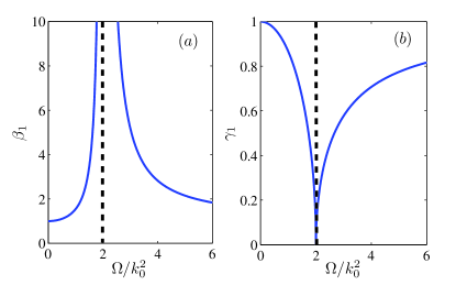
Figure 1: The corrections of the normal density [panel (a)] and the second sound velocity [panel (b)] in spin-orbit coupled BEC (along the $x$-axis direction). Note that near the phase transition ($\Omega/k_{0}^{2}\rightarrow 2$), the effective mass would diverge, i.e., $z_{1}\rightarrow\infty$.

IV.2 Superfluid density and Josephson relation

With the above linearized hydrodynamic equations, in the following we give a unified derivation for superfluid density and Josephson relation in spin-orbit coupled BEC. We should stress that one can take two different viewpoints on the effects of enhancement of effective mass in Eq. (IV.1). The first one is that the particle number density does not change, while the superfluid velocity decreases due to a factor $1/z_{1}$, which is adopted by previous sections in this paper. The another one is that the superfluid density decreases, while the superfluid velocity does not change, which would be adopted in following parts in this subsection.

We introduce superfluid density along the $\hat{q}$-direction $\rho_{s}(\hat{q})$ as

$$\rho_{s}(\hat{x})=n/z_{1},~{}\rho_{s}(\hat{y})=\rho_{s}(\hat{z})\equiv\rho_{s\perp}=n,$$

$$\rho_{s}(\hat{q})=\rho_{sx}\cos^{2}(\alpha)+\rho_{s\perp}\sin^{2}(\alpha).$$ (64)

In this case, Eq. (IV.1) becomes

$$\partial_{t}\delta n=-\rho_{s}(\hat{x})\partial_{x}^{2}\delta\theta-\rho_{s\perp}(\partial_{y}^{2}+\partial_{z}^{2})\delta\theta,$$

$$-\partial_{t}\delta\theta=g\delta n.$$ (65)

In the following, we will show that $\rho_{s}(\hat{q})$ is indeed the superfluid density.

We can write down an effective Hamiltonian for the hydrodynamic equation (IV.2) as

$$H_{\text{eff}} = \frac{1}{2}\int d^{3}\mathbf{r}\{\rho_{s}(\hat{x})(\partial_{x}\delta\theta)^{2}$$ (66)

$$+\rho_{s\perp}\left[(\partial_{y}\delta\theta)^{2}+(\partial_{z}\delta\theta)^{2}\right]+g(\delta n)^{2}\}.$$

Assuming the commutator relation $\left\{\delta\theta(\mathbf{r}),\delta n(\mathbf{r^{\prime}})\right\}=-\delta^{3}(\mathbf{r}-\mathbf{r}^{\prime})$ holds (Poisson brackets), we can easily get the above hydrodynamic equation (IV.2) from the Hamilton’s equations, i.e.,

$$\partial_{t}\delta n(\mathbf{r})=\{\delta n(\mathbf{r}),H_{\text{eff}}\},\partial_{t}\delta\theta(\mathbf{r})=\{\delta\theta(\mathbf{r}),H_{\text{eff}}\}.$$

Further assuming the quantized commutator relation $\left[\delta\theta(\mathbf{r}),\delta n(\mathbf{r}^{\prime})\right]=-i\delta^{3}(\mathbf{r}-\mathbf{r}^{\prime})$ holds Lifshitz , the phase $\delta\theta$ and density $\delta n$ can be be expressed in terms of the phonon’s annihilation and creation operators

$$\delta\theta(\mathbf{r},t)\!\!=\!\!\sum_{\mathbf{q}}\left[A_{\mathbf{q}}C_{\mathbf{q}}e^{i(\mathbf{q}\cdot\mathbf{r}-\omega_{\mathbf{q}}t)}+A_{\mathbf{q}}^{\ast}C_{\mathbf{q}}^{\dagger}e^{-i(\mathbf{q}\cdot\mathbf{r}-\omega_{\mathbf{q}}t)}\right],$$

$$\delta n(\mathbf{r},t)\!\!=\!\!\sum_{\mathbf{q}}\left[B_{\mathbf{q}}C_{\mathbf{q}}e^{i(\mathbf{q}\cdot\mathbf{r}-\omega_{\mathbf{q}}t)}+B_{\mathbf{q}}^{\ast}C_{\mathbf{q}}^{\dagger}e^{-i(\mathbf{q}\cdot\mathbf{r}-\omega_{\mathbf{q}}t)}\right],$$

where $A_{\mathbf{q}}(B_{\mathbf{q}})$ is a coefficient to be determined and $C_{\mathbf{q}}$ is the annihilation operator for phonon. From the continuity equation

$$\partial_{t}\delta n=-\rho_{s}(\hat{x})\partial_{x}^{2}\delta\theta-\rho_{s\perp}(\partial_{y}^{2}+\partial_{z}^{2})\delta\theta,$$

we get

$$-ic(\hat{q})B_{q}=q\rho_{s}(\hat{q})A_{q}.$$

From the commutator relation $\left[\delta\theta(\mathbf{r}),\delta n(\mathbf{r}^{\prime})\right]=-i\delta^{3}(\mathbf{r}-\mathbf{r}^{\prime})$, we get $A_{\mathbf{q}}B_{\mathbf{q}}^{\ast}=-i/2$ and then $A_{\mathbf{q}}=\sqrt{c(\hat{q})/\left[2\rho_{s}(\hat{q})q\right]}$, $B_{\mathbf{q}}=i\sqrt{\rho_{s}(\hat{q})q/\left[2c(\hat{q})\right]}$. Finally, we have

$$\delta\theta(\mathbf{r},t)\!\!=\!\!\sum_{\mathbf{q}}\sqrt{\frac{c(\hat{q})}{2\rho_{s}(\hat{q})q}}\left[C_{\mathbf{q}}e^{i(\mathbf{q}\cdot\mathbf{r}-\omega_{q}t)}+C_{\mathbf{q}}^{\dagger}e^{-i(\mathbf{q}\cdot\mathbf{r}-\omega_{\mathbf{q}}t)}\right],$$

$$\delta n(\mathbf{r},t)\!\!=\!\!i\sum_{\mathbf{q}}\sqrt{\frac{\rho_{s}(\hat{q})q}{2c(\hat{q})}}\left[C_{\mathbf{q}}e^{i(\mathbf{q}\cdot\mathbf{r}-\omega_{q}t)}-C_{\mathbf{q}}^{\dagger}e^{-i(\mathbf{q}\cdot\mathbf{r}-\omega_{\mathbf{q}}t)}\right].$$ (67)

From Eq. (67), we get density and phase fluctuations in terms of phonon’s operators as

$$n_{\mathbf{q}}=i\sqrt{\frac{\rho_{s}(\hat{q})q}{2c(\hat{q})}}\left(C_{\mathbf{q}}-C_{-\mathbf{q}}^{\dagger}\right),$$

$$\theta_{\mathbf{q}}=\sqrt{\frac{c(\hat{q})}{2\rho_{s}(\hat{q})q}}\left(C_{\mathbf{q}}+C_{-\mathbf{q}}^{\dagger}\right).$$ (68)

From Eq. (68), we can verify that $\rho_{s}(\hat{q})$ is indeed the superfluid density. For example, the superfluid density can be written as normaldensity

$$\rho_{s}(\hat{q}) = c^{2}(\hat{q})\kappa(\hat{q})$$ (69)

$$= \lim_{q\rightarrow 0}\frac{|\langle\mathbf{q}|n_{-\mathbf{q}}|0\rangle|^{2}\omega_{\mathbf{q}}+|\langle-\mathbf{q}|n_{\mathbf{q}}|0\rangle|^{2}\omega_{\mathbf{q}}}{q^{2}},$$

where

$$\kappa(\hat{q})=\lim_{q\rightarrow 0}\left[\frac{|\langle\mathbf{q}|n_{\mathbf{q}}^{\dagger}|0\rangle|^{2}}{c(\hat{q})q}+\frac{|\langle-\mathbf{q}|n_{-\mathbf{q}}^{\dagger}|0\rangle|^{2}}{c(\hat{q})q}\right]$$

is the compressibility, $|0\rangle$ is the ground state, and $|\mathbf{q}\rangle=C_{\mathbf{q}}^{\dagger}|0\rangle$ is the single-phonon state. In Eq. (69), we have used the fact that the single-phonon’s contribution is dominant in the compressibility normaldensity and $\omega_{\pm\mathbf{q}}=c(\hat{q})q$. Due to influences of upper branch, in spin-orbit coupled BEC, the superfluid density $\rho_{s}(\hat{q})$ would be smaller than the total density, i.e., $\rho_{s}(\hat{q})<n$ normaldensity . In this sense, we can interpret that the suppression of superfluid density in spin-orbit coupled BEC is due to the enhancement of effective mass.

On the other hand, as $q\rightarrow 0$ and at low energy, the boson field operator can be written as Lifshitz

$$\psi_{\sigma}(\mathbf{r})=\langle\psi_{\sigma}\rangle e^{i\delta\theta(\mathbf{r})}\simeq\langle\psi_{\sigma}\rangle\left[1+i\delta\theta(\mathbf{r})\right].$$

So we get

$$\psi_{\sigma,\mathbf{q}}=i\langle\psi_{\sigma}\rangle\theta_{\mathbf{q}}=i\langle\psi_{\sigma}\rangle\sqrt{\frac{c(\hat{q})}{2\rho_{s}(\hat{q})q}}\left[C_{\mathbf{q}}+C_{-\mathbf{q}}^{\dagger}\right].$$ (70)

With Eq. (70), the matrix element $\langle 0|\psi_{\sigma,\mathbf{q}}|\mathbf{q}\rangle=i\langle\psi_{\sigma}\rangle\sqrt{\frac{c(\hat{q})}{2\rho_{s}(\hat{q})q}}$, $\langle-\mathbf{q}|\psi_{\sigma,\mathbf{q}}|0\rangle=i\langle\psi_{\sigma}\rangle\sqrt{\frac{c(\hat{q})}{2\rho_{s}(\hat{q})q}}$, and the Green’s function matrix $G_{\sigma,\sigma}(\mathbf{q},0)=-\sum_{n}\left[\frac{\langle 0|\psi_{\sigma\textbf{q}}|n\rangle\langle n|\psi^{{\dagger}}_{\sigma\mathbf{q}}|0\rangle}{\omega_{n0}}+\frac{\langle 0|\psi^{{\dagger}}_{\sigma\mathbf{q}}|n\rangle\langle n|\psi_{\sigma\mathbf{q}}|0\rangle}{\omega_{n0}}\right]\simeq-\frac{|\langle\psi_{\sigma}\rangle|^{2}}{\rho_{s}(\hat{q})q^{2}}$ as $q\rightarrow 0$ zhangyicai2018 . In the above derivations, we have also used the fact that the single-phonon states have dominant contributions in the Green’s function as $\mathbf{q}\rightarrow 0$ and excitation energies for single-phonon states $\omega_{n0}=\omega_{\pm\mathbf{q}}=c(\hat{q})q$. Using $n_{0}=\sum_{\sigma={1,2}}|\langle\psi_{\sigma}\rangle|^{2}$, the Josephson relation is obtained zhangyicai2018

$$\rho_{s}(\hat{q})=-\lim_{q\rightarrow 0}\frac{n_{0}}{q^{2}trG(\mathbf{q},0)}.$$ (71)

The superfluid density from the Josephson relation [Eq. (71)] is also consistent with the current-current correlation calculations normaldensity .

From Eq. (70) of $\psi_{\sigma,\textbf{q}}$, we get the momentum distribution function as $q\rightarrow 0$,

$$N_{\mathbf{q}}=\sum_{\sigma=1,2}\langle\psi_{\sigma,\mathbf{q}}^{\dagger}\psi_{\sigma,\mathbf{q}}\rangle=\frac{n_{0}c(\hat{q})}{2\rho_{s}(\hat{q})q}\left(2n_{\mathbf{q}}+1\right),$$

where $n_{\mathbf{q}}=1/\left(e^{\omega_{\mathbf{q}}/T}-1\right)$ is the phonon Bose distribution function for the rest frame. Specially, at $T=0$ and as $q\rightarrow 0$, $N_{\mathbf{q}}=n_{0}c(\hat{q})/\left[2\rho_{s}(\hat{q})q\right]\propto 1/q$; when $\omega_{\mathbf{q}}\ll T$, $N_{\mathbf{q}}=n_{0}T/\left[\rho_{s}(\hat{q})q^{2}\right]\propto 1/q^{2}$, which are generalizations of the isotropic results Bogoliubov ; Lifshitz .

Using the effective Hamiltonian (66), we can calculate the phase or density fluctuations within the hydrodynamic formalism Pitaevskii . The energy in the momentum space is given by

$$\delta E=H_{\text{eff}}=\frac{1}{2}\int d^{3}\mathbf{r}\left\{\rho_{s}(\hat{x})(\partial_{x}\delta\theta)^{2}\right.$$

$$+\left.\rho_{s\perp}\left[(\partial_{y}\delta\theta)^{2}+(\partial_{z}\delta\theta)^{2}\right]+g(\delta n)^{2}\right\}$$

$$=\frac{1}{2}\sum_{\mathbf{q}}\left[\rho_{s}(\hat{q})q^{2}|\theta_{\mathbf{q}}|^{2}+g|n_{\mathbf{q}}|^{2}\right].$$ (72)

Because the thermal probability distribution

$$P\propto e^{-\delta E/T}=e^{-\frac{1}{2}\sum_{\mathbf{q}}\left[\rho_{s}(\hat{q})q^{2}|\theta_{\mathbf{q}}|^{2}+g|n_{\mathbf{q}}|^{2}\right]/T},$$

for the long wave lengths ($\omega_{\mathbf{q}}\ll T$), the thermal fluctuations of the phase and density are given by

$$\langle|\theta_{\mathbf{q}}|^{2}\rangle=\frac{T}{\rho_{s}(\hat{q})q^{2}}\text{, \ }\langle|n_{\mathbf{q}}|^{2}\rangle=\frac{T}{g}.$$

Along the $x$-axis direction ($\hat{q}=\hat{x}$), we see the phase fluctuation near phase transition point [$\rho_{s}(\hat{x})\rightarrow 0$] is very dramatic and diverges, while the density fluctuation is always finite.

V Conclusion

In summary, we have generalized the two-fluid theory to a superfluid system with anisotropic effective masses. As a specific example, this theory is used to investigate spin-orbit coupled BEC realized in recent experiments. At low temperature, the normal density from phonon excitations and the second sound velocity have been obtained analytically. Near the phase transition from the plane wave to zero-momentum phases, due to the effective mass divergence, the normal density from phonon excitation increases greatly, while the second sound velocity is suppressed significantly. With quantum hydrodynamic formalism, we have given a unified derivation for the suppressed superfluid density and Josephson relation.

Before ending up this paper, we make three remarks. The first is that our previous calculations are restricted to the case of $z>1$. However, our theory can be extended straightforwardly to the other case of $0<z<1$. The main results are similar and thus are not discussed here. The second is that for the spin-coupled BEC at higher temperature, the up gapped excitation would play an important role in hydrodynamics. Thus, how to take account of the up branch excitations properly and construct corresponding hydrodynamic theory still needs further investigations. The last is that when the system is exactly at the phase-transition point from the plane-wave and zero momentum phases, the quadratic effective mass terms ($\propto p^{2}$) in the Hamiltonian (15) would vanish, while quartic terms ($\propto p^{4}$) may play an important role. In such case, the corresponding hydrodynamics also needs further investigations.

VI Acknowledgements

Yi-Cai Zhang thank Shizhong Zhang for useful discussions. This work was supported by the NSFC under Grants No. 11874127, No. 11674200, No. 11747079, No. 61565007, No. 11875149, No. 61565013, No. 11434015 and No. 61835013, the National Key R&D Program of China under grants No. 2016YFA0301500, SPRPCAS under grants No. XDB01020300 and No.XDB21030300, and Hong Kong Research Grants Council (General Research Fund, Grant No. HKU 17318316 and Collaborative Research Fund, Grant No. C6026-16W). Yi-Cai Zhang also acknowledge the support of a startup grant from Guangzhou University.

References

• (1) L. Tisza, Transport phenomena in Helium II, Nature (London) 141, 913 (1938).
• (2) L. Landau, The theory of superfluidity of Helium II, J. Phys. U. S. S. R. 5, 71 (1941).
• (3) E. Taylor and A. Griffin, Two-fluid hydrodynamic modes in a trapped superfluid gas, Phys. Rev. A 72, 053630 (2005).
• (4) Y. He, Q. Chen, C.-C. Chien, and K. Levin, First- and second-sound-like modes at finite temperature in trapped Fermi gases from BCS to BEC, Phys. Rev. A 76, 051602(R) (2007).
• (5) E. Taylor, H. Hu, X.-J. Liu, L. P. Pitaevskii, A. Griffin, and S. Stringari, First and second sound in a strongly interacting Fermi gas, Phys. Rev. A 80, 053601 (2009).
• (6) Y.-H. Hou, L. P. Pitaevskii, and S. Stringari, First and second sound in a highly elongated Fermi gas at unitarity, Phys. Rev. A 88, 043630 (2013).
• (7) H. Hu, P. Dyke, C. J. Vale, and X.-J. Liu, First and second sound of a unitary Fermi gas in highly oblate harmonic traps, New J. Phys. 16, 083023 (2014).
• (8) R. Meppelink, S. B. Koller, and P. van der Straten, Sound propagation in a Bose-Einstein condensate at finite temperatures, Phys. Rev. A 80, 043605 (2009).
• (9) M. K. Tey, L. A. Sidorenkov, E. R. S. Guajardo, R. Grimm, M. J. H. Ku, M. W. Zwierlein, Y.-H. Hou, L. Pitaevskii, and S. Stringari, Collective Modes in a Unitary Fermi Gas across the Superfluid Phase Transition, Phys. Rev. Lett. 110, 055303 (2013).
• (10) M. R. Andrews, D. M. Kurn, H.-J. Miesner, D. S. Durfee, C. G. Townsend, S. Inouye, and W. Ketterle, Propagation of Sound in a Bose-Einstein Condensate, Phys. Rev. Lett. 79, 553 (1997).
• (11) J. Joseph, B. Clancy, L. Luo, J. Kinast, A. Turlapov, and J. E. Thomas, Measurement of Sound Velocity in a Fermi Gas near a Feshbach Resonance, Phys. Rev. Lett. 98, 170401 (2007).
• (12) V. B. Shenoy and T.-L. Ho, First and Second Sound Modes of a Bose-Einstein Condensate in a Harmonic Trap, Phys. Rev. Lett. 80, 3895 (1998).
• (13) E. Zaremba, A. Griffin, and T. Nikuni, Two-Fluid Hydrodynamics for a Trapped Weakly-Interacting Bose Gas, Phys. Rev. A 57, 4695 (1998).
• (14) H. Heiselberg, Sound modes at the BCS-BEC crossover, Phys. Rev. A 73, 013607 (2006).
• (15) E. Arahata and T. Nikuni, Propagation of second sound in a superfluid Fermi gas in the unitary limit, Phys. Rev. A 80, 043613 (2009).
• (16) G. Baym and C. J. Pethick, Normal mass density of a superfluid Fermi gas at unitarity, Phys. Rev. A 88, 043631 (2013).
• (17) L. A. Sidorenkov, M. K. Tey, R. Grimm, Y.-H. Hou, L. Pitaevskii, and S. Stringari, Second sound and the superfluid fraction in a Fermi gas with resonant interactions, Nature (London) 498, 78 (2013).
• (18) S. Riedl, E. R. S. Guajardo, C. Kohstall, J. H. Denschlag, and R. Grimm, Superfluid quenching of the moment of inertia in a strongly interacting Fermi gas, New J. Phys. 13, 035003 (2011).
• (19) Y. J. Lin, K. J. García, and I. B. Spielman, Spin-orbit-coupled Bose-Einstein condensates, Nature (London) 471, 83 (2011).
• (20) P. Wang, Z.-Q. Yu, Z. Fu, J. Miao, L. Huang, S. Chai, H. Zhai, and J. Zhang, Spin-Orbit Coupled Degenerate Fermi Gases, Phys. Rev. Lett. 109, 095301 (2012).
• (21) L. W. Cheuk, A. T. Sommer, Z. Hadzibabic, T. Yefsah, W. S. Bakr, and M. W. Zwierlein, Spin-Injection Spectroscopy of a Spin-Orbit Coupled Fermi Gas, Phys. Rev. Lett. 109, 095302 (2012).
• (22) J.-Y. Zhang, S.-C. Ji, Z. Chen, L. Zhang, Z.-D. Du, B. Yan, G.-S. Pan, B. Zhao, Y.-J. Deng, H. Zhai, S. Chen, and J.-W. Pan, Collective Dipole Oscillations of a Spin-Orbit Coupled Bose-Einstein Condensate, Phys. Rev. Lett. 109, 115301 (2012).
• (23) A. J. Olson, S.-J. Wang, R. J. Niffenegger, C.-H. Li, C. H. Greene, and Y. P. Chen, Tunable Landau-Zener transitions in a spin-orbit coupled Bose-Einstein condensate, Phys. Rev. A 90, 013616 (2014).
• (24) M. A. Khamehchi, Y. Zhang, C. Hamner, T. Busch, and P. Engels, Measurement of collective excitations in a spin-orbit-coupled Bose-Einstein condensate, Phys. Rev. A 90, 063624 (2014).
• (25) T. L. Ho and S. Zhang, Bose-Einstein Condensates with Spin-Orbit Interaction, Phys. Rev. Lett. 107, 150403 (2011).
• (26) Y.-C. Zhang, Z.-Q. Yu, T. K. Ng, S. Zhang, L. Pitaevskii, and S. Stringari, Superfluid density of a spin-orbit-coupled Bose gas, Phys. Rev. A 94, 033635 (2016).
• (27) S. Stringari, Diffused vorticity and moment of inertia of a spin-orbit coupled Bose-Einstein condensate, Phys. Rev. Lett. 118, 145302 (2017).
• (28) G. I. Martone, Y. Li, L. P. Pitaevskii, and S. Stringari, Anisotropic dynamics of a spin-orbit coupled Bose-Einstein condensate, Phys. Rev. A 86, 063621 (2012).
• (29) C. Qu, L. P. Pitaevskii, and S. Stringari, Spin-orbit-coupling induced localization in the expansion of an interacting Bose-Einstein condensate, New J. Phys. 19, 085006 (2017).
• (30) M. A. Khamehchi, K. Hossain, M. E. Mossman, Y. Zhang, T. Busch, M. M. Forbes, and P. Engels, Negative-Mass Hydrodynamics in a Spin-Orbit-Coupled Bose-Einstein Condensate, Phys. Rev. Lett. 118, 155301 (2017).
• (31) P. M. Chaikin and T. C. Lubensky, Principles of condensed matter physics (Cambridge University Press, Cambridge, 1995).
• (32) Y.-H. Hou and Z. Yu, Hydrodynamics of Normal Atomic Gases with Spin-orbit Coupling, Sci. Rep. 5, 15307 (2015).
• (33) L. D. Landau and E. M. Lifshitz, Course of theoretical Physics Volume 6 Fluid mechanics (Academic,London, 2ed, 1987).
• (34) I. M. Khalatnikov, An Introduction to the Theory of Superfluidity (W. A. Benjamin, N.Y., 1965).
• (35) L. Pitaevskii and S. Stringari, Bose-Einstein Condensation (Oxford University Press, 2003).
• (36) D. Pines and P. Nozières, The theory of Quantum Liquids, Vol. 2 (Addison-Wesley, Redwood City, 1990).
• (37) H. Hu, E. Taylor, X.-J. Liu, S. Stringari, and A. Griffin, Second sound and the density response function in uniform superfluid atomic gases, New J. Phys. 12, 043040 (2010).
• (38) M.G. Lingham, K. Fenech, S. Hoinka, and C.J. Vale, Local Observation of Pair Condensation in a Fermi Gas at Unitarity, Phys. Rev. Lett. 112, 100404 (2014).
• (39) K. R. Atkins, Liquid Helium, chapter 3, page 67 (Cambridge University Press, Cambridge, 1959).
• (40) V. Pastukhov, Infrared Behavior of Dipolar Bose Systems at Low Temperatures, J. Low Temp. Phys. 186, 148 (2017).
• (41) V. Pastukhov, Beyond mean-field properties of binary dipolar Bose mixtures at low temperatures, Phys. Rev. A 95, 023614 (2017).
• (42) Q. Zhu, C. Zhang, and B. Wu, Exotic superfluidity in spin-orbit coupled Bose-Einstein condensates. Eur. Phys. Lett. 100, 50003 (2012).
• (43) W. Zheng, Z. Q. Yu, X. Cui and H. Zhai. Properties of Bose Gases with Raman-Induced Spin-Orbit Coupling, J. Phys. B 46, 134007 (2013).
• (44) Y. Li, L. P. Pitaevskii, and S. Stringari, Quantum tri-criticality and phase transitions in spin-orbit coupled Bose-Einstein condensates, Phys. Rev. Lett. 108, 225301 (2012).
• (45) C. Wang, C. Cao, C. M. Jian, and H. Zhai, Spin-Orbit Coupled Spinor Bose-Einstein Condensates. Phys. Rev. Lett. 105, 160403 (2010).
• (46) S. K. Yip, Bose-Einstein condensation in the presence of artificial spin-orbit interaction, Phys. Rev. A 83, 043616 (2011).
• (47) S.-C. Ji, L. Zhang, X.-T. Xu, Z. Wu, Y. Deng, S. Chen, and J.-W. Pan, Softening of Roton and Phonon Modes in a Bose-Einstein Condensate with Spin-Orbit Coupling, Phys. Rev. Lett. 114, 105301 (2015).
• (48) W. Zheng and Z. Li, Collective modes of a spin-orbit-coupled Bose-Einstein condensate: A hydrodynamic approach, Phys. Rev. A 85, 053607 (2012).
• (49) E. M. Lifshitz and L. P. Pitaevskii, Course of theoretical Physics Volume 9 Statistical Physics part 2, Chapter III (Academic,London, 1980).
• (50) Y.-C. Zhang, Generalized Josephson relation for conserved charges in multicomponent bosons, Phys. Rev. A 98, 033611 (2018).
• (51) N. N. Bogoliubov, Lectures on Quantum Statistics (Gordon and Breach, New York, 1970).