Topological magnon bands for magnonics

Abstract

Topological excitations in magnetically ordered systems have attracted much attention lately. We report on topological magnon bands in ferromagnetic Shastry-Sutherland lattices whose edge modes can be put to use in magnonic devices. The synergy of Dzyaloshinskii-Moriya interactions and geometrical frustration are responsible for the topologically nontrivial character. Using exact spin-wave theory, we determine the finite Chern numbers of the magnon bands which give rise to chiral edge states. The quadratic band crossing point vanishes due the present anisotropies, and the system enters a topological phase. We calculate the thermal Hall conductivity as an experimental signature of the topological phase. Different promising compounds are discussed as possible physical realizations of ferromagnetic Shastry-Sutherland lattices hosting the required antisymmetric Dzyaloshinskii-Moriya interactions. Routes to applications in magnonics are pointed out.

Topological phases Hasan and Kane (2010); Qi and Zhang (2011) exist in both fermionic and bosonic systems and constitute a fast developing research area. Although the theoretical understanding of fermionic topological systems has made impressive progress, topological bosonic excitations have gained considerable attention only in the past few years. Despite the increasing conceptual knowledge of topological matter, only very few materials have been identified with topological properties compared to the large number of potential topological materials Bradlyn et al. (2017). Even less is known about potential applications. This is, in particular, true for topological bosonic signatures Onose et al. (2010). Thus, it is a major challenge to theoretically predict and experimentally verify topological bosonic fingerprints in order to move towards useful applications.

In the research of topological properties in condensed matter, the magnetic degrees of freedom have increased in importance. Magnetic data storage is already a ubiquitous everyday technology Fert (2008). Recently, magnetic spin waves, so-called magnons, themselves are used to carry and to process information which is called ” magnonics ” Shindou et al. (2013); Kruglyak et al. (2010); Demokritov and Slavin (2013). Adding topological aspects the field of magnonics Nakata et al. (2017a) considerably enhances the possibilities to build efficient devices for which we will make a proposal in this paper.

The challenge in finding topological signatures in magnetically ordered spin systems are the small Dzyaloshinskii-Moriya (DM) interactions Dzyaloshinsky (1958); Moriya (1960) which induce only small Berry curvatures. The size of the DM terms relative to the isotropic coupling is roughly as large as $|g-2|/2$, i.e., the deviation of the $g$ factor from 2, because both result from spin-orbit coupling. Thus, the DM terms are generically too small to induce detectable topological effects. In strongly frustrated systems, however, the relative size of the DM terms can indeed be comparable to the isotropic couplings Splinter et al. (2016).

Another issue is the localization of edge modes. Employing the wording of semiconductor physics, one must distinguish direct (at fixed wave vector) and indirect gaps (allowing for changes in the wave vector). The existence of direct gaps throughout the Brillouin zone (BZ) is sufficient to separate bands so that their topological properties are well defined. But the vanishing of the indirect gap generically implies that the edge states are not localized anymore, i.e., the bulk-boundary correspondence with respect to localization does not hold anymore Malki et al. (2018).

In magnetic systems, three types of elementary excitations occur. Long-range ordered magnets display magnons (or spin waves) Bloch (1930), valence-bond crystals mostly feature triplons Schmidt and Uhrig (2003), whereas quantum spin liquids may display fractional excitations Morris et al. (2009), for instance, spinons Faddeev and Takhtajan (1981). For triplons, topological behavior, i.e., non-zero Chern numbers Thouless et al. (1982), has been predicted Romhányi et al. (2015); Malki and Schmidt (2017) and verified McClarty et al. (2017) in Shastry-Sutherland lattices and in spin ladders Joshi and Schnyder (2017). For ferromagnetically ordered systems, topological magnons have been theoretically suggested in kagome lattices Katsura et al. (2010); Chisnell et al. (2015), pyrochlore lattices Zhang et al. (2013), and in honeycomb lattices Owerre (2016); Kim et al. (2016). For antiferromagnets, they have been proposed in pyrochlore lattices Li et al. (2016), square, and cubic lattices exploiting the Aharonov-Casher effect Nakata et al. (2017b). In analogy to the quantum Hall effect v. Klitzing et al. (1980), the magnon Hall effect Onose et al. (2010) as well as the triplon Hall effect Romhányi et al. (2015) arise since the topological Berry curvature acts analogously to a magnetic field. So far, only the magnon Hall effect has been observed Onose et al. (2010); Ideue et al. (2012). Topologically non-trivial spinons have been discussed in the Mott insulator Pesin and Balents (2010); Rachel and Le Hur (2010) as well as in quantum spin liquids Katsura et al. (2010); Rüegg and Fiete (2012); Cho et al. (2012).

The Shastry-Sutherland model Shastry and Sutherland (1981) is commonly studied with antiferromagnetic couplings leading to triplon excitations Miyahara and Ueda (2003). Including DM interactions combined with a transverse magnetic field induces topological properties Romhányi et al. (2015); Malki and Schmidt (2017) where the magnetic field is also used as a control parameter to tune topological phase transition. The Shastry-Sutherland lattice with purely ferromagnetic couplings serves also as a good platform but for topological magnon excitations. This is one of the two main objectives of this article; the second one is to discuss compounds which are likely to realize this model and to point out possible applications.

We show by exact spin-wave theory that the ferromagnetic Shastry-Sutherland model with DM couplings has topological bands with non-trivial Chern numbers. The occurrence of a ferromagnetic ground state represents the spontaneous breaking of time-reversal symmetry. In combination with the DM interactions a finite Berry curvature is induced which may lead to finite Chern numbers. The degeneracy at the quadratic band crossing point (QBCP) is lifted, and a gap opens. The expected topologically protected edge states Hatsugai (1993) are retrieved in strip geometry Malki and Uhrig (2017). In order to guide the experimental verification of the magnon Hall effect, we compute the thermal Hall effect as well.

Real materials are always three-dimensional ($3$D); so we look for the ferromagnetic Shastry-Sutherland model realized in various layers of $3$D materials. If the interlayer coupling sup is not too strong, the $3$D quantum Hall states can be considered as ensemble of layered two-dimensional ($2$D) quantum Hall states so that it is appropriate to investigate $2$D models.

Layers of the Shastry-Sutherland lattice are found in various insulating magnetic materials since it is easily constructed from corner-sharing squares. The squares are not aligned parallel or perpendicular to one other so that dimers are formed, see Fig. 1(a). Due to the lack of inversion symmetry about the midpoints of the bonds, DM interactions are possible and generically occur from spin-orbit interactions. To reach large values of the DM couplings, it is indicated to include atoms with large atomic numbers because large electron velocities favor relativistic effects. Moreover, the couplings should be ferromagnetic so that it is indicated to avoid linear bonds which would favor antiferromagnetic superexchange according to the Goodenough-Kanamori rules. Hence, the Shastry-Sutherland lattice depicted in Fig. 1 appears promising if superexchange via larger subgroups does not occur (this is what happens in SrCu2(BO3)2 Miyahara and Ueda (2003)). The following materials appear to be particularly interesting: RE5Si4 or RE Si Roger et al. (2006); Spichkin et al. (2001) (RE=Gd, Dy, Ho, Er, Y). The compounds RE5Si4 have a Sm5Ge4-type structure, and RESi has a FeB-type structure which both comprise planes of Shastry-Sutherland lattices. These compounds display a macroscopic magnetization $\mathbf{M}$ indicating dominant ferromagnetic couplings Spichkin et al. (2001); Roger et al. (2006). In addition, the macroscopic magnetization clearly shows that one of the two degenerate ground states dominates, i.e., one domain prevails.

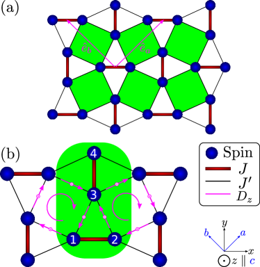
Figure 1: (a) Illustration of the $2$D Shastry-Sutherland lattice. The nearest neighbor couplings are shown as thick red lines, whereas the squares are highlighted in green. (b) The model studied comprises the Heisenberg couplings $J$ and $J^{\prime}$ as well as the DM interaction $D_{z}$. The unit cell is highlighted in green. The sequence of the spin in the term $\mathbf{D}_{z}\cdot\mathbf{S}_{i}\times\mathbf{S}_{j}$ is shown by the arrow pointing from $i$ to $j$. The DM couplings follow a clockwise rotation, see the circular arrows.

We compute the four bands from the unit cell with four sites shown in Fig. 1(b) in green. The DM couplings of the Shastry-Sutherland lattice can be directed in plane or out of plane Romhányi et al. (2015). Usually, however, the out-of-plane couplings dominate in 2D Romhányi et al. (2015); Chernyshev and Maksimov (2016). In order to focus on a minimal model, we thus constrain the DM coupling to a uniform direction perpendicular to the plane $\mathbf{D}=D_{z}\hat{e}_{z}$ as shown in Fig. 1(b). Obviously, this introduces a chiral orientation. Single-ion anisotropy (SIA) $A^{\alpha\beta}$ ($\alpha,\beta\in\left\{x,y,z\right\}$) is typically present in ferromagnets with spins $S>1/2$. For the minimal model, we consider it to favor easy-axis alignment along the $z$ axis $A^{zz}=A\geq 0$. The SIA and the DM coupling compete because the latter profits from tilts away from the $z$ axis. A conservative estimate sup shows that for small SIA and DM coupling the SIA wins and the fully polarized state is generic.

The complete Hamiltonian of the minimal model consists of three parts

$$\mathcal{H}= \mathcal{H}_{\mathrm{H}}+\mathcal{H}_{\mathrm{DM}}+\mathcal{H}_{\mathrm{SIA}}$$ (1a)

$$\mathcal{H}_{\mathrm{H}}= -J\sum_{\left\langle ij\right\rangle}\left[\frac{1}{2}(S_{i}^{+}S_{j}^{-}+S_{i}^{-}S_{j}^{+})+S_{i}^{z}S_{j}^{z}\right]$$

$$-J^{\prime}\!\!\sum_{\left\langle\left\langle ij\right\rangle\right\rangle}\!\left[\frac{1}{2}(S_{i}^{+}S_{j}^{-}+S_{i}^{-}S_{j}^{+})+S_{i}^{z}S_{j}^{z}\right]\!\!\!\!$$ (1b)

$$\mathcal{H}_{\mathrm{DM}}= -\frac{\mathrm{i}D_{z}}{2}\sum_{\left\langle\left\langle ij\right\rangle\right\rangle}(S_{i}^{+}S_{j}^{-}-S_{i}^{-}S_{j}^{+})$$ (1c)

$$\mathcal{H}_{\mathrm{SIA}}= -A\sum_{i}(S_{i}^{z})^{2},$$ (1d)

with ferromagnetic couplings $J,J^{\prime}>0$; $J$ serves as the energy unit henceforth. A pair of nearest neighbors and of next-nearest neighbors is denoted by ${\left\langle ij\right\rangle}$ and by ${\left\langle\left\langle ij\right\rangle\right\rangle}$, respectively.

We use the Dyson-Maleev representation of the spin operators Dyson (1956); Maleev (1957) which is exact as long as a single magnon above the fully polarized ground state is considered. But even for several magnons, spin-wave theory is well justified due to the large spins involved ($S\approx 4-5$ for $\left\{\ce{RE=Gd},\ce{Dy},\ce{Ho},\ce{Er},\ce{Y}\right\}$). Note that large spins generically lead to large energy ranges with considerable gaps which are favorable for application. The bilinear Hamiltonian in momentum space reads

$$\mathcal{H}=\sum_{\mathbf{k}}\sum_{nm}b_{n,\mathbf{k}}^{\dagger}\mathcal{M}_{nm}^{\phantom{\dagger}}(\mathbf{k})b_{m,\mathbf{k}}^{\phantom{\dagger}}$$ (2)

where $b_{n}^{\dagger}$ and $b_{n}^{\phantom{\dagger}}$ are the bosonic creation and annihilation operators at the site $n\in\left\{1,2,3,4\right\}$, see Fig. 1(b). The $4\times 4$ Hamiltonian matrix is given by

$$\underline{\underline{\mathcal{M}}}(\mathbf{k})=\begin{pmatrix}\underline{\underline{A}}&\underline{\underline{B}}(k_{a},k_{b})\\ \underline{\underline{B}}^{\dagger}(k_{a},k_{b})&\underline{\underline{A}}\end{pmatrix},$$ (3)

with the $2\times 2$ matrices,

$$\underline{\underline{A}} =\begin{pmatrix}JS+4J^{\prime}S+A(2S-1)\quad\qquad-JS\\ -JS\quad\qquad JS+4J^{\prime}S+A(2S-1)\end{pmatrix}$$ (4a)

$$\underline{\underline{B}} =\begin{pmatrix}-C^{\phantom{*}}(1+e^{\mathrm{i}k_{a}})&-C^{*}(e^{\mathrm{i}k_{a}}+e^{\mathrm{i}(k_{a}+k_{b})})\\ -C^{*}(1+e^{\mathrm{i}k_{b}})&-C^{\phantom{*}}(e^{\mathrm{i}k_{b}}+e^{\mathrm{i}(k_{a}+k_{b})})\end{pmatrix}\!\!\!\!\!\!$$ (4b)

where $C:=S(J^{\prime}+\mathrm{i}D_{z})$. We set the lattice constant to unity so that the wave vectors become dimensionless. Diagonalizing $\mathcal{M}(\mathbf{k})$ yields four distinct magnon bands $\mathcal{H}=\sum_{n,\mathbf{k}}\omega_{n}(\mathbf{k})\tilde{b}^{\dagger}_{n,\mathbf{k}}\tilde{b}^{\phantom{\dagger}}_{n,\mathbf{k}}$ depicted in Fig. 2. The four bands come in pairs $p$ of two bands which are degenerate on the boundary of the BZ. We strongly presume that this degeneracy is linked to the composite point symmetry of the Shastry-Sutherland lattice which consists of a vertical or horizontal translation shifting vertical dimers to horizontal ones and vice versa combined with a rotation by 90^∘. But we did not find analytic proof. The whole lattice is $C_{4}$ symmetric considering rotations about the centers of the squares so that dispersions display the same symmetry.

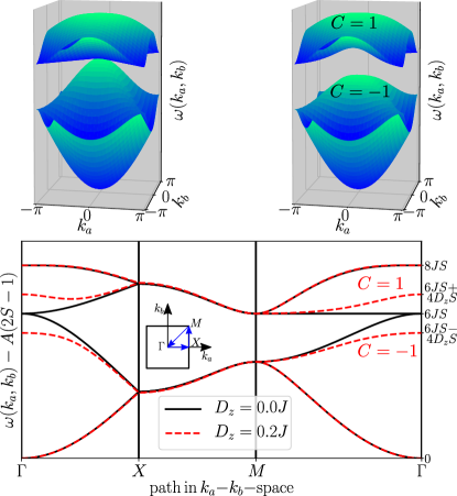
Figure 2: One-magnon dispersions for $J=J^{\prime}$ for two values of the DM coupling. The critical case is $D_{z}=0$ (upper left panel and black lines in the lower panel) where the QBCP at the $\Gamma$ point is clearly visible. The degeneracy of the quadratic bands is lifted for finite $D_{z}>0$ (upper right panel and red lines in the lower panel) so that distinct bands appear which show non-trivial topological Chern numbers $C=\pm 1$.

Ferromagnetic Heisenberg models without spin anisotropic couplings, such as SIA or DM coupling display gapless Goldstone bosons Goldstone (1961) with a quadratic dispersion at low energies at the $\Gamma$ point. As soon as the SIA $A$ is turned, on the continuous spin rotation symmetry is no longer broken spontaneously but externally, and a finite spin gap $A(2S-1)$ appears; note the offset energy axis in the lower panel of Fig. 2. Spontaneously, the system chooses one of the two degenerate fully polarized ground states. This stabilizes the fully polarized ground state since it becomes energetically isolated from the remaining spectrum.

For vanishing DM coupling, two magnon bands cross quadratically at the $\Gamma$ point at finite energies. Hence, the model displays an unusual QBCP. Linear Dirac cones Haldane (1988) or variants of them Romhányi et al. (2015) are more standard. Generically, one can assign a Berry phase of $\pi$ (or multiples of $\pi$) to them Sun et al. (2009). The QBCP is stable and can be interpreted as a pair of Dirac cones Chong et al. (2008) which are superimposed due to the $C_{4}$ symmetry Sun et al. (2009). As a result, a QBCP can have a Berry flux of $0$ or $\pm 2\pi$. The QBCP can either be removed by breaking the $C_{4}$ symmetry which splits it into an even number of Dirac cones or by lifting its degeneracy, e.g., by opening a gap leading to topologically non-trivial bands. Turning on the DM interaction ($D_{z}\neq 0$) induces the latter scenario. But as shown in Fig. 2, the degeneracy of the upper pair of bands and of the lower pair of bands at the boundary of the BZ persists so that no Chern number of a single band can be defined. Hence, one defines the Chern number of subspaces by taking the trace over the Berry curvature in each subspace Soluyanov and Vanderbilt (2012); Malki and Schmidt (2017) which derives from the Berry phase of the determinants of unitary transformations along closed paths Uhrig (1991). Denoting the Chern number of a pair of bands by $C^{(p)}$ where $p$ stands for ‘upper’ or ‘lower’ one has

$$C^{(p)}=\frac{1}{2\pi}\iint_{\rm BZ}\sum_{n\in p}\left[F_{n,ab}({\bf k})\;\right]\;{\rm d}k_{a}\;{\rm d}k_{b}\,,$$ (5)

where $F_{n,ab}$ is the Berry curvature of band $n$ defined by

$$F_{n,ab}({\bf k}) =\frac{\partial A_{n,b}({\bf k})}{\partial k_{a}}-\frac{\partial A_{n,a}({\bf k})}{\partial k_{b}}$$ (6a)

$$\mathrm{with}\quad A_{n,\mu}(\mathbf{k}) =\langle\mathbf{k},n|\nabla_{k_{\mu}}|\mathbf{k},n\rangle\,.$$ (6b)

The numerical robust calculation of the Berry curvature is performed by discretization of the BZ Fukui et al. (2005) avoiding the eigenstates precisely at the boundaries of the BZ. This is possible because the relevant curvature occurs in the vicinity of the $\Gamma$ point anyway. The calculated Chern numbers of the pairs of magnon bands is $C^{(\text{upper/lower})}=\pm 1$ as shown in Fig. 2. Changing the sign of the $D_{z}$ reverses the sign of the Chern numbers. The non-zero Chern numbers can be attributed to the complex hopping stemming from the DM coupling leading to fluxes of fictitious fields Katsura et al. (2010); Ideue et al. (2012). The direct gap between both pairs of bands occurs at $\Gamma$ and is given by $8D_{z}S$ as long as $4D_{z}<J$. Otherwise, the direct gap is located at the $M$ point and takes the value $2JS$. These relations highlight the importance of large spins and DM couplings for large gaps.

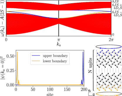
Figure 3: (Upper panel) Eigen energies of a strip geometry, see the lower right panel with $N=50$, $J=J^{\prime}$, $D_{z}=0.2J$, and $A=0.2J$. (Lower left panel) Probability density $|\psi(k_{a}=0,r_{b})|^{2}$ as a function of site $r_{b}$ of both edge modes; the color of their curves corresponds to the color of the boundary sites in the lower right panel.

According to the bulk-boundary correspondence Hatsugai (1993); Thouless et al. (1982), the existence of nontrivial Chern numbers implies topologically protected edge states Mook et al. (2014). For verification, we analyze a finite strip of $N=50$ unit cells in the $b$ direction and periodic boundaries in the $a$ direction, see the lower right panel in Fig. 3. The energy eigen values as a function of the well-defined wave-vector $k_{a}$ are depicted in the upper panel of Fig. 3. One can easily see two chiral edge states moving right and left according to the slope of their dispersion branches which connect the two continua shown in red. Additionally, the lower left panel illustrates the localization of these modes at the lower (yellow curve and sites) and upper (blue curve and sites) edge of the strip.

Next, we address possible experimental signatures. Since magnons do not carry charge, usual electric conductivity measurements do not make sense. The thermal Hall effect offers a way to detect nontrivial Berry curvatures in real materials. The thermal Hall effect consists of a finite-temperature gradient perpendicular to a heat current. The expression for the transversal heat conductivity $\kappa_{ab}$ Matsumoto and Murakami (2011) is given by

$$\kappa_{ab}=-\frac{k_{B}^{2}T}{\hbar}\sum_{n,\bf k}c_{2}(\rho_{n})F_{n,ab}(\bf k)$$ (7)

where we sum over all magnon bands and set $k_{B}=1$ and $\hbar=1$. The weight $c_{2}(\rho_{n})$ is given by

$$c_{2}(\rho) =\left.\int_{\varepsilon_{n}}^{\infty}\mathrm{d}\varepsilon\left(\beta\varepsilon\right)^{q}\left(-\frac{\mathrm{d}\rho}{\mathrm{d}\varepsilon}\right)\right|_{\mu=0}$$ (8a)

$$=-2\,\mathrm{Li}_{2}(-\rho)+\rho\ln^{2}(\rho^{-1}+1)-\ln^{2}(\rho+1)$$

$$\phantom{=}+2\ln(\rho+1)\ln(\rho^{-1}+1)\,,$$ (8b)

where $\rho$ is the Bose-Einstein distribution $(\exp(\beta\omega)-1)^{-1}$ and $\mathrm{Li}_{m}$ is the dilogarithm for $m=2$ (Spence’s integral, in general). Equation (7) clearly shows that the transversal heat conductivity $\kappa_{ab}$ depends directly on the Berry curvature, thus, representing an ideal fingerprint of non-trivial topological properties. Figure 4 displays the results of Eq. (7) as a function of temperature for various values of $D_{z}$. For the topological phase ($D_{z}\neq 0$), the conductivity first slightly decreases to negative values before it strongly increases as a function of temperature. For high temperatures, $\kappa_{ab}$ approaches a finite value. In comparison, the topologically trivial bands for $D_{z}=0$ may have a finite curvature, but such that it cancels in the sum over the BZ so that $\kappa_{ab}$ vanishes.

Since the magnetization generally decreases with increasing temperature untill eventually the ferromagnetic phase ceases to exist at $T_{c}$, $\kappa_{ab}$ should also decrease until it disappears at $T_{c}$. By improving the calculations by applying self-consistent spin-wave theory, the signature starts to decrease for higher temperatures before no self-consistent solution is found anymore as depicted by the dashed lines sup .

In conclusion, a finite thermal Hall conductivity $\kappa_{ab}$ can serve as a smoking gun signature in experiments to verify topological properties of a material under study. For large signals, we suggest the experimental preparation of a single domain crystal in order to avoid cancellation effects.

Figure 4: Thermal Hall conductivity $\kappa_{ab}$ as a function of temperature for various values of the DM coupling $D_{z}$ at $J=J^{\prime},$ $A=0.2J$, and $S=4$.

In view of the above findings, we suggest characterizing the magnetic properties of the putative realizations Spichkin et al. (2001); Roger et al. (2006) of ferromagnetic Shastry-Sutherland lattices in detail, for instance, by inelastic neutron scattering. This will help to determine the relevant microscopic model which, in turn, will render the calculation of the Berry curvature possible. In parallel, measurements of the thermal Hall conductivity can provide evidence Onose et al. (2010); Ideue et al. (2012) for finite Berry curvatures.

The intriguing next step towards an application will be to tailor the edges of strip by decorating them similar to what has been proposed and computed for fermionic models Uhrig (2016); Malki and Uhrig (2017). In this way, largely different group velocities can be achieved depending on the direction in which signals of packets of magnons travel. The key is to structure the upper and the lower boundaries of a strip in a different manner so that the group velocity of the right- and of the left-moving packet is very different. Ideally, the group velocities should be tunable by moderate changes of the model controlled by external parameters, such as magnetic fields or pressure. The realization of this phenomenon will pave the way for fascinating devices in magnonics, such as delay lines and interference devices.

Estimate of the competition between the single-ion anisotropy and the Dzyaloshinskii-Moriya interaction

Here we estimate up to which value of the Dzyaloshinskii-Moriya (DM) interaction the collinear, fully polarized ferromagnetic order favored by the single-ion anisotropy (SIA) represents the ground state of the model. To obtain such an estimate we study two next-nearest neighbor spins coupled by $J^{\prime}$ as classical vectors of length $S$ with polar angles $\theta_{1}$ and $\theta_{2}$ and relative azimuthal angle $\varphi:=\varphi_{1}-\varphi_{2}$ which takes the value $\tan\varphi=d:=D_{z}/J^{\prime}$ at the energy minimum $E$

$$2E/(J^{\prime}S^{2})=-a(1+xy)/2-x-y-|x-y|\sqrt{1+d^{2}}$$ (S1)

where $a:=A/J^{\prime}$, $x:=\cos(\theta_{1}+\theta_{2})$, and $y:=\cos(\theta_{1}-\theta_{2})$ with $|x|,|y|\leq 1$. The SIA term $a$ is split into four parts $a/4$ because each site has four $J^{\prime}$ bonds. As long as $1+a/2\geq\sqrt{1+d^{2}}$ full polarization is optimum, i.e., a canted state can occur for $d\geq\sqrt{a+a^{2}/4}$ only, which is a conservative estimate because the effects of $J$, of quantum fluctuations, and of the geometric constraints in the lattice are not included. Hence, for small SIA and DM coupling the SIA wins and the fully polarized state is generic.

Effects of interlayer couplings

In absence of detailed information about the structure and the magnetic couplings in the discussed three-dimensional (3D) materials we elucidate that the effect of weak interlayer couplings do not destroy the topological properties put forward in the main text.

To this end, we assume that the system consists of stacked parallel planes present where each plane realizes a two-dimensional (2D) ferromagnetic Shastry-Sutherland model. The distinct planes are connected by a perpendicular interlayer coupling $J_{c}$. Since there is no detailed data on magnetic exchange paths for the proposed classes of materials Roger et al. (2006); Spichkin et al. (2001) we restrict the calculations to vertical couplings between the layers because they usually have the largest impact. As a result, the Hamiltonian Eq. (1) is extended by the additional term

$$\mathcal{H}_{\mathrm{inter}}=-J_{c}\sum_{\left\langle ij\right\rangle}\left[\frac{1}{2}(S_{i}^{+}S_{j}^{-}+S_{i}^{-}S_{j}^{+})+S_{i}^{z}S_{j}^{z}\right]$$ (S2)

with the ferromagnetic coupling $J_{c}>0$. The notation $\left\langle ij\right\rangle$ indicates a coupling between nearest neighbors from adjacent layers. We apply the Dyson-Maleev representation Dyson (1956); Maleev (1957) and the Fourier transform to calculate the dispersion of the bosonic one-particle excitations within spin wave theory which is exact for the excitations above the fully polarized ferromagnetic state. In this way, the interlayer term $\mathcal{H}_{\mathrm{inter}}$ results to an additional $4\times 4$-matrix given by $4J_{c}S\sin^{2}(k_{c}^{2}/2)\mathbbm{1}$, i.e., proportional to the identity matrix.

From this we conclude that the ground states remains fully polarized since the finite spin gap remains at its value $A(2S-1)$ created by the SIA. The topological properties in the bulk remain the same as well because terms proportional to the identity matrix obviously do not change the eigen states. Since only the eigen states determine the topological properties the same Chern number will ensue, regardless of the strength of $J_{c}$, at each value of $k_{c}$.

Concomitantly, we find edge states in the corresponding strip geometry for arbitrary $k_{c}$. The resulting dispersion is the same as shown in Fig. 3 (in the main text) with an additional overall shift proportional to $4J_{c}S\sin^{2}(k_{c}^{2}/2)$. The localization of the 3D edge states is identical due to the one of the 2D eigen states. The set of all localized edge states depending on $k_{a}$ and $k_{c}$ represent surface states.

In conclusion, the investigation of additional 3D perpendicular interlayer coupling shows that the topological edge modes persist and are not altered as long as the fully polarized ground state is preserved. Hence, for weak interlayer coupling the topological properties found in the two-dimensional model also hold in three dimensions and thus the proposed materials are good candidates to search for realizations.

Self-consistent spin wave theory

The temperature dependency of the static calculation of the transversal heat conductivity $\kappa_{ab}$ stems only from the weight $c_{2}(\rho_{n})$ and its contribution to $\kappa_{ab}$ which is proportional to the Berry curvature $F_{n,ab}(\mathbf{k})$. This curvature, however, is independent of temperature. In order to make quantitative statements, it is appropriate to improve the results for finite temperatures, i.e., to include partly the effects of finite $T$.

Here we use the Dyson-Maleev representation of the spin operators which leads to an exact description at quartic level and is given by

$$S_{i}^{+} =\sqrt{2S}(b_{i}^{\phantom{\dagger}}-\frac{1}{2S}b_{i}^{\dagger}b_{i}^{\phantom{\dagger}}b_{i}^{\phantom{\dagger}})$$ (S3)

$$S_{i}^{-} =\sqrt{2S}\phantom{(}b_{i}^{\dagger}$$ (S4)

$$S_{i}^{z} =b_{i}^{\dagger}b_{i}^{\phantom{\dagger}}-S\,.$$ (S5)

The complete Hamiltonian in the bosonic representation is then described by

$$\mathcal{H}= \mathcal{H}_{\mathrm{H}}+\mathcal{H}_{\mathrm{DM}}+\mathcal{H}_{\mathrm{SIA}}$$ (S6a)

$$\mathcal{H}_{\mathrm{H}}= -J\sum_{\left\langle ij\right\rangle}S(b_{i}^{\dagger}b_{j}^{\phantom{\dagger}}+b_{j}^{\dagger}b_{i}^{\phantom{\dagger}}-b_{i}^{\dagger}b_{i}^{\phantom{\dagger}}-b_{j}^{\dagger}b_{j}^{\phantom{\dagger}})$$ (S6b)

$$+J\sum_{\left\langle ij\right\rangle}\frac{1}{2}(b_{i}^{\dagger}b_{i}^{\dagger}b_{i}^{\phantom{\dagger}}b_{j}^{\phantom{\dagger}}+b_{j}^{\dagger}b_{j}^{\dagger}b_{j}^{\phantom{\dagger}}b_{i}^{\phantom{\dagger}})-b_{i}^{\dagger}b_{j}^{\dagger}b_{i}^{\phantom{\dagger}}b_{j}^{\phantom{\dagger}}\!\!\!\!$$

$$-J^{\prime}\!\!\sum_{\left\langle\left\langle ij\right\rangle\right\rangle}\!S(b_{i}^{\dagger}b_{j}^{\phantom{\dagger}}+b_{j}^{\dagger}b_{i}^{\phantom{\dagger}}-b_{i}^{\dagger}b_{i}^{\phantom{\dagger}}-b_{j}^{\dagger}b_{j}^{\phantom{\dagger}})$$ (S6c)

$$+J^{\prime}\!\!\sum_{\left\langle\left\langle ij\right\rangle\right\rangle}\frac{1}{2}(b_{i}^{\dagger}b_{i}^{\dagger}b_{i}^{\phantom{\dagger}}b_{j}^{\phantom{\dagger}}+b_{j}^{\dagger}b_{j}^{\dagger}b_{j}^{\phantom{\dagger}}b_{i}^{\phantom{\dagger}})-b_{i}^{\dagger}b_{j}^{\dagger}b_{i}^{\phantom{\dagger}}b_{j}^{\phantom{\dagger}}\!\!\!\!$$

$$\mathcal{H}_{\mathrm{DM}}= -\mathrm{i}D_{z}\sum_{\left\langle\left\langle ij\right\rangle\right\rangle}S(b_{i}^{\dagger}b_{j}^{\phantom{\dagger}}+b_{j}^{\dagger}b_{i}^{\phantom{\dagger}})$$

$$+\frac{\mathrm{i}D_{z}}{2}\sum_{\left\langle\left\langle ij\right\rangle\right\rangle}(b_{i}^{\dagger}b_{i}^{\dagger}b_{i}^{\phantom{\dagger}}b_{j}^{\phantom{\dagger}}+b_{j}^{\dagger}b_{j}^{\dagger}b_{j}^{\phantom{\dagger}}b_{i}^{\phantom{\dagger}})$$ (S6d)

$$\mathcal{H}_{\mathrm{SIA}}= -A\sum_{i}(2S-1)b_{i}^{\dagger}b_{i}^{\phantom{\dagger}}+b_{i}^{\dagger}b_{i}^{\dagger}b_{i}^{\phantom{\dagger}}b_{i}^{\phantom{\dagger}}\,,$$ (S6e)

where we neglected all constant terms. Applying a mean field decoupling reduces the quartic terms into bilinear terms. For this purpose we introduce the expectation values

$$n =\left\langle b_{i}^{\dagger}b_{i}^{\phantom{\dagger}}\right\rangle\in\mathbb{R}$$ (S7a)

$$a =\left\langle b_{i}^{\dagger}b_{j}^{\phantom{\dagger}}\right\rangle\in\mathbb{R}\quad\mathrm{for}\left\langle ij\right\rangle$$ (S7b)

$$c =\left\langle b_{i}^{\dagger}b_{j}^{\phantom{\dagger}}\right\rangle\in\mathbb{C}\quad\mathrm{for}\left\langle\left\langle ij\right\rangle\right\rangle\,,$$ (S7c)

where $a$ corresponds to nearest neighbors and $c$ to next-nearest neighbors. The Fourier transformation of the mean field Hamiltonian yields

$$\mathcal{H}=\sum_{\mathbf{k}}\sum_{nm}b_{n,\mathbf{k}}^{\dagger}\mathcal{M}_{nm}^{\phantom{\dagger}}(\mathbf{k},n,a,c)\,b_{m,\mathbf{k}}^{\phantom{\dagger}}$$ (S8)

with the bosonic creation $b_{n}^{\dagger}$ and annihilation operators $b_{n}^{\phantom{\dagger}}$ at the site $n\in\left\{1,2,3,4\right\}$. The Hamiltonian becomes implicitly temperature dependent since the expectation values are depending on temperature. The $4\times 4$ Hamilton matrix reads

$$\underline{\underline{\mathcal{M}}}(\mathbf{k})=\begin{pmatrix}\underline{\underline{A}}&\underline{\underline{B}}(k_{a},k_{b})\\ \underline{\underline{B}}^{\dagger}(k_{a},k_{b})&\underline{\underline{A}}\end{pmatrix}$$ (S9)

with the $2\times 2$ matrices

$$\underline{\underline{A}}=\begin{pmatrix}A_{11}&A_{12}\\ A_{21}&A_{22}\\ \end{pmatrix}\qquad\underline{\underline{B}}=\begin{pmatrix}B_{11}&B_{12}\\ B_{21}&B_{22}\\ \end{pmatrix}\!\!\!\!\!\!$$ (S10)

$$A_{11} =A_{22}=J(S-n+a)+4J^{\prime}(S-n+\mathrm{Re}(c))+A(2S-4n-1)+4D_{z}\mathrm{Im}(c)$$ (S11a)

$$A_{12} =A_{21}=-J(S-n+a)$$ (S11b)

$$B_{11} =-J^{\prime}(S-n+c^{*})-J^{\prime}(S-n+c)e^{\mathrm{i}k_{a}}-\mathrm{i}D_{z}(S-n)(1+e^{\mathrm{i}k_{a}})$$ (S11c)

$$B_{21} =-J^{\prime}(S-n+c^{*})-J^{\prime}(S-n+c)e^{\mathrm{i}k_{b}}+\mathrm{i}D_{z}(S-n)(1+e^{\mathrm{i}k_{b}})$$ (S11d)

$$B_{12} =-J^{\prime}(S-n+c)e^{\mathrm{i}k_{a}}-J^{\prime}(S-n+c^{*})e^{\mathrm{i}(k_{a}+k_{b})}+\mathrm{i}D_{z}(S-n)(e^{\mathrm{i}k_{a}}+e^{\mathrm{i}(k_{a}+k_{b})})$$ (S11e)

$$B_{22} =-J^{\prime}(S-n+c)e^{\mathrm{i}k_{b}}-J^{\prime}(S-n+c^{*})e^{\mathrm{i}(k_{a}+k_{b})}-\mathrm{i}D_{z}(S-n)(e^{\mathrm{i}k_{b}}+e^{\mathrm{i}(k_{a}+k_{b})})$$ (S11f)

By expressing the expectation values using the Bose-Einstein distribution we are able to determine self-consistently the renormalized dispersion and the corresponding magnetization $m$ at a specific temperature. The magnetization is given by the simple relation $m=S-n$. The renormalized spin gap $\Delta$ is purely determined by the SIA being given by

$$\Delta=A(2S-4n-1).$$ (S12)

Obviously, the spin gap closes before the magnetization vanishes, so that in this approximation a Curie temperature cannot be determined. The spin gap closes for $2S-4n-1=0$. For the magnetization this implies that the spin gap closes if the magnetization reaches the value $m=(2S+1)/4$ as indicated by the horizontal dashed line in Fig. S1.

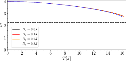
Figure S1: Magnetization as a function of temperature $T$ for various $D_{z}$ at $J=J^{\prime},A=0.2J,$ and $S=4$. The horizontal dashed line indicates the value at which the spin gap closes.

The self-consistently calculated magnetization shows the unexpected problem that no solution can be found even before the spin gap closes or the magnetization vanishes. It appears that the phase transition from the ordered phase induced by the SIA to the disordered phase cannot be captured by spin wave theory. This issue deserves further investigations, but it is beyond the scope of the present article.

References

- Roger et al. (2006) J. Roger, V. Babizhetskyy, T. Guizouarn, K. Hiebl, R. Guérin, and J.-F. Halet, J. Alloys and Compounds 417, 72 (2006).
- Spichkin et al. (2001) Y. I. Spichkin, V. K. Pecharsky, and K. A. Gschneidner, Jr., J. Appl. Phys. 89, 1738 (2001).
- Dyson (1956) F. J. Dyson, Phys. Rev. 102, 1217 (1956).
- Maleev (1957) S. V. Maleev, Zh. Eksp. Teor. Fiz. 33, 1010 (1957).