Mechanical relaxation and fracture of phase field crystals

Abstract

A computational method is developed for the study of mechanical response and fracture behavior of phase field crystals (PFC), to overcome a limitation of the PFC dynamics which lacks an effective mechanism for describing fast mechanical relaxation of the material system. The method is based on a simple interpolation scheme for PFC (IPFC) making use of a condition of the displacement field to satisfy local elastic equilibration, while preserving key characteristics of the original PFC model. We conduct a systematic study on the mechanical properties of a sample nanoribbon system with honeycomb lattice symmetry subjected to uniaxial tension, for numerical validation of the IPFC scheme and the comparison with the original PFC and modified PFC methods. Results of mechanical response, in both elasticity and fracture regimes, show the advantage and efficiency of the IPFC method across different system sizes and applied strain rates, due to its effective process of mechanical equilibration. A brittle fracture behavior is obtained in IPFC calculations, where effects of system temperature and chirality on the fracture strength and Young’s modulus are also identified, with results agreeing with those found in previous atomistic simulations of graphene. The IPFC scheme developed here is generic and applicable to the mechanical studies using different types of PFC free energy functionals designed for various material systems.

I Introduction

The mechanical properties of materials, including their strength, fracture behavior, and elastic properties, are among the key factors determining the technological applications of the material system. A recent example is the exploration of novel two-dimensional (2D) monolayer materials such as graphene, which is known as one of the strongest materials being made. Both experimental Lee et al. (2008) and computational Zhao et al. (2009); Zhao and Aluru (2010); Grantab et al. (2010); Liu et al. (2007); Zakharchenko et al. (2009) efforts have been devoted to the study of its mechanical and fracture behaviors under various sample conditions such as system temperature, chirality, defects, sample size, imposed strain rate, and crack length.

Computational studies of these material mechanical behaviors are often relied upon the use of atomistic simulation techniques, including molecular dynamics (MD) Zhao et al. (2009); Zhao and Aluru (2010); Grantab et al. (2010), first-principles density functional theory (DFT) Liu et al. (2007), and Monte Carlo (MC) Zakharchenko et al. (2009) methods. These atomistic methods are usually characterized by the microscopic length and atomic vibration time scales, and thus are limited by the small system sizes and short dynamic time ranges that they can access. Although such constraints on spatial and temporal scales can be significantly relieved by the use of continuum approaches, the traditional continuum theories, such as phase field models and continuum elasticity theory, lack the explicit details of atomic-level crystalline microstructures that are important for determining the mechanical and fracture properties of material systems particularly those beyond the elasticity regime.

To overcome this difficulty in materials modeling, one of recent efforts has been put on combining the microscopic crystalline details with continuum density-field formulation, in particular the development of phase field crystal (PFC) models Elder et al. (2002); Elder and Grant (2004); Stefanovic et al. (2006); Greenwood et al. (2010); Mkhonta et al. (2013); Wang et al. (2018) which have attracted large amounts of recent research interest and resulted in a wide range of applications such as the study of solidification Elder and Grant (2004); Greenwood et al. (2010); Mkhonta et al. (2013), defect structures and dynamics Berry et al. (2006); Taha et al. (2017); Adland et al. (2013); Salvalaglio et al. (2018); Skaugen et al. (2018a), crystal nucleation and grain growth Wu and Voorhees (2012); Tóth et al. (2010); Guo et al. (2018), surface ordering and patterns Elder et al. (2016); Smirman et al. (2017), mechanical behavior or crack dynamics Stefanovic et al. (2006, 2009); Zhou et al. (2017); Gao et al. (2016); Hu et al. (2017), among many others. Although the PFC method has the advantage of being able to address large length and time scales without losing atomic spatial resolution of the microstructure, the standard dynamics of PFC is characterized only by slow, diffusive time scales for all the system dynamical processes (including the elastic relaxation). It thus lacks a separate mechanism for elastic and mechanical response, for which the relaxation process occurs on much smaller phonon-level time scales or almost instantaneously (i.e., with instantaneous mechanical equilibrium), a feature that is particularly important for the study of material mechanical behavior and fracture.

This drawback of PFC dynamics can be partially remedied by incorporating the damped wave modes into the PFC equation, i.e., the modified PFC (MPFC) model Stefanovic et al. (2006, 2009) which, however, is still limited by the associated effective length scale of elastic interaction and by its stricter requirement of numerical convergence in computation. The model is also subjected to a restriction on the fastness of system dynamics it can achieve Heinonen et al. (2016a). In principle, the dynamics of mechanical relaxation should be examined through the details of acoustic phonon modes. The incorporation of them in the PFC framework has been derived via the Poisson bracket formalism Majaniemi and Grant (2007), and usually manifests in terms of hydrodynamic couplings (see, e.g., the hydrodynamic models Baskaran et al. (2016); Tóth et al. (2014) based on classical DFT of freezing and the Navier-Stokes equation), although further work is needed to identify the effect and computational efficiency of these models on the mechanical relaxation processes. Recently much attention has been paid to the construction of amplitude equation formulation for PFC, with two methods developed to address the issue of fast elastic relaxation Heinonen et al. (2016b, a, 2014). The first one is through imposing a separate, extra condition of elastic equilibration (via the phases of complex amplitudes) on the standard overdamped, dissipative dynamics governing the slowly varying amplitudes of the density field Heinonen et al. (2014). In the second method hydrodynamic coupling is introduced to the PFC amplitude formulation, such that the elastic relaxation is determined by large-wavelength phonon modes Heinonen et al. (2016b, a). Both methods can well produce the fast dynamics for mechanical equilibration, but the corresponding slow-scale amplitude description does not incorporate the coupling to the underlying microscopic lattice structure and thus lacks the resulting lattice pinning effect Huang (2013) and Peierls barriers for defect motion Berry et al. (2006), which are needed for understanding the mechanical behavior of materials. In addition, a very recent study showed that an additional smooth distortion field and the associated compatible strain should be incorporated into PFC to obtain full mechanical equilibrium of the system Skaugen et al. (2018b). The method is based on linear elasticity and is to be extended to the nonlinear elasticity regime. In short, so far a complete PFC-type dynamics that can cover the full range of system characteristic time and length scales and the real material evolution processes (ranging from fast elastic to slow diffusive relaxation) is still lacking, and the solution is elusive given the coarse-grained nature (in both space and time) of the PFC-type density field approach.

In this work we introduce an alternative, effective computational scheme for PFC mechanical relaxation, via imposing an additional constraint on the original PFC model by assuming that after each step of mechanical deformation, the system would instantaneously adjust to a state close to local elastic equilibrium and then relax from this new initial state to reach the mechanical equilibration. It is achieved by a simple interpolation algorithm for the PFC density field, based on the property of linear spatial dependence of atomic displacements under small strain increment in between two subsequent deformation steps. This facilitates a rapid relaxation to the mechanical equilibrium state of the system even with the use of standard diffusive PFC dynamics. The validity and high efficiency of this method are verified through the study of uniaxial tensile test on a sample double-notched nanoribbon system with 2D honeycomb lattice symmetry. Effects of system size, strain rate, temperature, and structure chirality have been systematically examined, with results of mechanical response and fracture compared to the calculations using the original PFC and MPFC models, to demonstrate the advantage of this interpolation scheme of PFC (IPFC) particularly for large system sizes and a broad range of strain rates.

II Models and Method

II.1 PFC and MPFC models

In the original PFC model for single-component systems Elder et al. (2002); Elder and Grant (2004), the dimensionless free energy functional is given by

$$F=\int d\vec{r}\left\{\frac{\phi}{2}[r+(\nabla+1)^{2}]\phi+\frac{\tau}{3}\phi^{3}+\frac{1}{4}\phi^{4}\right\},$$ (1)

where the order parameter $\phi$ represents the variation of the atomic number density field from a constant reference value, and $r$ and $\tau$ are phenomenological parameters. The equilibrium thermodynamic properties of the PFC model can be controlled by varying the temperature parameter $r$ and the average atomic density Elder and Grant (2004), showing a transition between the homogeneous (or liquid) phase to the spatially periodic, crystalline solid state. In a crystalline solid phase, the order parameter field $\phi$ can be written in a general form:

$$\phi(\vec{r})=\phi_{0}+\sum_{n,m}A_{nm}e^{i\vec{G}_{nm}\cdot\vec{r}},$$ (2)

where $\phi_{0}$ is the average atomic density variation, $A_{nm}$ are the amplitudes, and $\vec{G}_{nm}=n\vec{b}_{1}+m\vec{b}_{2}$, with $(n,m)$ the Miller indices and $(\vec{b}_{1},\vec{b}_{2})$ the principle reciprocal lattice vectors. For the example of a 2D lattice with hexagonal symmetry, we have

$$\vec{b}_{1}=q_{0}\left(\frac{\sqrt{3}}{2}\hat{x}+\frac{1}{2}\hat{y}\right),\qquad\vec{b}_{2}=q_{0}\hat{y},$$ (3)

where $q_{0}={2\pi}/(a_{0}\sqrt{3}/2)$ with the lattice constant $a_{0}$. Within the one-mode approximation $(n,m)=(\pm 1,0)$, $(0,\pm 1)$, and $(\pm 1,\mp 1)$, $A_{\pm 10}=A_{\pm 1\mp 1}\equiv A_{\rm eq}$, $A_{0\pm 1}=-A_{\rm eq}$, and thus

$$\phi=\phi_{0}+2A_{\rm eq}\left[2\cos\left(\frac{\sqrt{3}}{2}q_{0}x\right)\cos\left(\frac{1}{2}q_{0}y\right)-\cos(q_{0}y)\right].$$ (4)

In the equilibrium state determined by the free energy minimization, $q_{0}=1$, and when $\tau+3\phi_{0}>0$,

$$A_{\rm eq}=-\frac{1}{15}\left(\tau+3\phi_{0}+\sqrt{\tau^{2}-15r-24\tau\phi_{0}-36\phi_{0}^{2}}\right),$$ (5)

corresponding to a 2D honeycomb lattice as will be examined below. Note that it is essentially the inverse of triangular phase in one-mode PFC Elder et al. (2016).

The standard PFC dynamics is of dissipative nature and governed by the conserved, time-dependent Ginzburg-Landau equation $\partial\phi/\partial t=\nabla^{2}\delta F/\delta\phi$, which leads to

$$\frac{\partial\phi}{\partial t}=\nabla^{2}\left[r\phi+(\nabla^{2}+1)^{2}\phi+\tau\phi^{2}+\phi^{3}\right].$$ (6)

The corresponding system evolution are then controlled by diffusive dynamics, even for processes that are related to much faster time scales such as elastic or plastic relaxation and mechanical response. To overcome this shortcoming, the above PFC dynamics has been modified by adding a wave-mode term of second order time derivative Stefanovic et al. (2006), so that two different time scales of the diffusional and elastic or phonon-type modes can be incorporated, i.e.,

$$\frac{\partial^{2}\phi}{\partial t^{2}}+\beta\frac{\partial\phi}{\partial t}=\alpha^{2}\nabla^{2}\left[r\phi+(\nabla^{2}+1)^{2}\phi+\tau\phi^{2}+\phi^{3}\right],$$ (7)

where $\alpha$ is proportional to the speed of sound wave and $\beta$ is a phenomenological parameter associated with the damping rate. It is important to know that in this MPFC model, the fast elastic propagating behavior is limited within an effective elastic interaction range that is proportional to $\alpha/\beta$ Stefanovic et al. (2006, 2009), beyond which the diffusive dynamics (similar to that of original PFC) dominates. Also, recent analysis indicated that although the elastic interaction range can always be increased by reducing the $\beta$ value, beneath a certain threshold of $\beta$ the system dynamics cannot be further accelerated Heinonen et al. (2016a). Such limitations play an important role on the size effect and computational efficiency for the simulation of system mechanical response, as will be demonstrated below.

II.2 Modeling of systems under uniaxial tension

To model a PFC or MPFC system subjected to a uniaxial tension, we use the traction boundary conditions introduced in Refs. Stefanovic et al. (2006, 2009) by adding an additional energy penalty term $F_{\rm ext}$ into the free energy functional Eq. (1), which effectively fixes the density field of the loaded and moving boundary layers (the traction regions) to a pre-defined field $\phi_{\rm trac}$ representing the corresponding equilibrium crystal structure, i.e.,

$$F_{\rm ext}=\int d{\vec{r}}M(\vec{r})\left[\phi(\vec{r})-\phi_{\rm trac}(\vec{r})\right]^{2}.$$ (8)

Here the traction function $M(\vec{r})$ is set to be a positive constant ($=2$) within the traction regions that are moved with a specific strain rate $\dot{\varepsilon}$, and is zero outside the regions. In our simulations $\phi_{\rm trac}$ is chosen as the equilibrium profile of the traction regions determined numerically before the imposing of tension.

A schematic of the corresponding system setup for mechanical deformation is given in Fig. 1. What is illustrated there is an example system consisting of two types of crystalline regions (blue and green) surrounded by a coexisting homogeneous phase (white margins). The solid sample is stretched vertically along the $y$ direction at both ends, with the tensile load applied on seven rows of atoms at each end (green; traction regions with $M(\vec{r})>0$). The mechanical relaxation occurs in the middle solid region (blue; active zone with $M(\vec{r})=0$), which is configured as a double notched single-crystal nanoribbon for our tests. Before the application of the uniaxial tension, the whole system is relaxed to reach an equilibrium state which is used as the initial condition of the subsequent tensile test, with the initial lengths of the active zone denoted as $L_{x}^{0}$ and $L_{y}^{0}$ in the $x$ and $y$ directions, respectively. For the example of Fig. 1, the total system size is $256\Delta x\times 512\Delta y$, while the initial active region of the nanoribbon is measured as $L_{x}^{0}\times L_{y}^{0}=196\Delta x\times 340\Delta y$. Various system sizes have been used in our simulations, all with similar system setup.

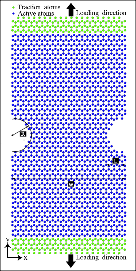
Figure 1: Schematic of a 2D double notched single-crystal nanoribbon subjected to a uniaxial tensile loading.

To identify the mechanical properties during the tensile test, we calculate the strain energy of the nanoribbon as $F_{s}=F(\varepsilon_{e})-F(\varepsilon_{e}=0)$, where $\varepsilon_{e}=(L_{y}-L_{y}^{0})/L_{y}^{0}$ is the applied engineering strain, with $L_{y}$ the strained length of the active zone along the stretching direction. The engineering stress is calculated by

$$\sigma_{e}=\frac{1}{\mathcal{A}_{0}}\frac{\partial F_{s}}{\partial\varepsilon_{e}}=\frac{1}{\dot{\varepsilon}}\frac{\partial(F_{s}/\mathcal{A}_{0})}{\partial t},$$ (9)

where the initial area $\mathcal{A}_{0}=L_{x}^{0}\times L_{y}^{0}$, $F_{s}/\mathcal{A}_{0}$ is the strain energy density, and $\dot{\varepsilon}$ is the strain rate. During each tensile loading step, the nanoribbon is stretched by a minimum increment of one grid spacing $\Delta y$ at each end, resulting in a strain increment of $\Delta\varepsilon_{e}=2\Delta y/L_{y}^{0}$. If this stretching increment is imposed every $N$ time steps (i.e., every $N\Delta t$ of time), we have

$$\dot{\varepsilon}=\frac{\Delta\varepsilon_{e}}{N\Delta t}=\frac{2\Delta y}{L_{y}^{0}N\Delta t}.$$ (10)

An extra attention needs to be paid to the time scale and hence the strain rate for the wave-mode MPFC model as compared to the diffusive PFC dynamics. In the original PFC model Eq. (6), the associated time scale can be determined via that of vacancy diffusion, $\tau_{D}=a_{0}^{2}/D$ Berry et al. (2006), where $a_{0}$ is the lattice spacing [$a_{0}=4\pi/(\sqrt{3}q_{0})$ in PFC] and $D$ is the vacancy diffusion constant determined by $D=1+r+2\tau\phi_{0}+3\phi_{0}^{2}+18A_{\rm eq}^{2}$ Elder and Grant (2004). If labeling all the corresponding dimensional variables or parameters by a superscript “$d$” to distinguish from the dimensionless quantities in the PFC equations, we can identify the PFC time scale as

$$\left.\frac{t^{d}}{t}\right|_{\rm PFC}=\frac{\tau_{D}^{d}}{\tau_{D}}=\left(\frac{a_{0}^{d}}{a_{0}}\right)^{2}\left(\frac{D}{D^{d}}\right),$$ (11)

where $a_{0}^{d}$ and $D^{d}$ are the lattice spacing and vacancy diffusion constant of the specific real material to be studied. On the other hand, in MPFC governed by the wave dynamic Eq. (7), the vacancy diffusion is characterized by an effective diffusion coefficient $D_{\rm MPFC}=\alpha^{2}(1+r+2\tau\phi_{0}+3\phi_{0}^{2}+18A_{\rm eq}^{2})/\beta=(\alpha^{2}/\beta)D$ Stefanovic et al. (2006), leading to a MPFC time scale

$$\left.\frac{t^{d}}{t}\right|_{\rm MPFC}=\left(\frac{a_{0}^{d}}{a_{0}}\right)^{2}\left(\frac{D_{\rm MPFC}}{D^{d}}\right)=\frac{\alpha^{2}}{\beta}\left.\frac{t^{d}}{t}\right|_{\rm PFC},$$ (12)

an increase by a factor of $\alpha^{2}/\beta$ compared to the PFC time scale. Thus this factor needs to be incorporated into the strain rate calculation in MPFC, i.e.,

$$\dot{\varepsilon}_{\rm MPFC}=\frac{2\beta\Delta y}{\alpha^{2}L_{y}^{0}N\Delta t},$$ (13)

to be comparable with the PFC strain rate Eq. (10).

II.3 An interpolation scheme for mechanical relaxation

As discussed above, a key factor for effectively modeling the mechanical response of a system is to achieve fast (or close to instantaneous) elastic relaxation in system dynamics, which is the motivation behind the recent development of MPFC Stefanovic et al. (2006, 2009) and amplitude Heinonen et al. (2014, 2016b, 2016a) methods. Here we introduce a simple, alternative algorithm to efficiently facilitate the rapid process of strain relaxation in systems under mechanical deformation. It makes use of a property of linear elasticity assuming the linear spatial dependence of the displacement field $u_{y}$ when reaching mechanical equilibrium, given a small strain increment $\Delta\varepsilon$ imposed by each stretching step, i.e.,

$$u_{y}\cong\Delta\varepsilon(y-y^{*}),\qquad\Delta\varepsilon=2\Delta y/L_{y},$$ (14)

where the displacement $u_{y}$ is measured with respect to the positions at the beginning of each stretching step, so that after this stretching $y\rightarrow y+u_{y}$ and the strained length $L_{y}$ is increased by $2\Delta y$ given the two-end pulling. $\Delta\varepsilon$ represents the incremental strain in between two subsequent steps as a result of the new tensile loading, and $y^{*}$ is the central position of the stretched sample with zero displacement. [A similar setup can be used in the case of one-end pulling for which the fixed end is located at $y=y^{*}=0$ and thus $\Delta\varepsilon=\Delta y/L_{y}$ in Eq. (14).] Note that $\Delta\varepsilon$ is always very small since it accounts for the applied strain increase due to the stretching by only one grid spacing at each end, and thus Eq. (14) is a reasonably good approximation even beyond the stage of elasticity or close to the fracture regime. A corresponding one-dimensional (1D) schematic along the stretching $y$ direction is shown in Fig. 2, indicating (i) the fixed central grid point $j_{y}^{*}=y^{*}/\Delta y$, (ii) the grid positions $j_{y}=y/\Delta y$ before the current-step deformation (filled points), and (iii) the relaxed ones $j_{y}+\delta_{j_{y}}$ for $y>y^{*}$ and $j_{y}>j_{y}^{*}$, or $j_{y}-\delta_{j_{y}}$ for $y<y^{*}$ and $j_{y}<j_{y}^{*}$ after deformation (open points). Given Eq. (14), we have

$$\delta_{j_{y}}=|u_{y}|/\Delta y=\Delta\varepsilon|j_{y}-j_{y}^{*}|,$$ (15)

and $0<\delta_{j_{y}}<\Delta\varepsilon(L_{y}/2)/\Delta y=1$.

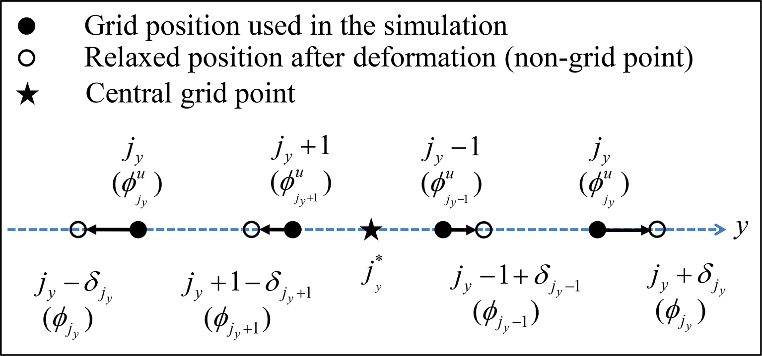
Figure 2: Schematic of mechanical deformation along the $y$ direction parallel to the uniaxial tensile loading. The star point indicates the grid position at the central line of the stretched nanoribbon. Note that the filled points shown here are the simulation grid points, but not necessarily the atomic lattice sites, while the open points indicate the corresponding relaxed positions after each step of deformation which, however, are not grid positions due to $0<\delta_{j_{y}}<1$.

Between two consecutive steps of tensile loading, assume $\phi_{j_{y}}$ is the “old” density field obtained from mechanical relaxation following the previous step (i.e., right before the new stretching), and $\phi^{u}_{j_{y}}$ is the updated density field at the same simulation grid position $j_{y}$ after the new tensile load. As a result of the strain-induced linear displacement described by Eqs. (14) and (15) with $y\rightarrow y+u_{y}$, we get $\phi(y)\rightarrow\phi^{u}(y+u_{y})$, i.e., $\phi^{u}_{j\pm\delta_{j_{y}}}=\phi_{j_{y}}$ (“$+$”: for $j_{y}>j_{y}^{*}$; “$-$”: for $j_{y}<j_{y}^{*}$). Note that $j\pm\delta_{j_{y}}$ is not a grid position used in numerical simulation due to $0<\delta_{j_{y}}<1$. We then determine the value of $\phi^{u}_{j_{y}}$ at any grid point $j_{y}$ by a linear interpolation either between $j_{y}-1+\delta_{j_{y}-1}$ and $j_{y}+\delta_{j_{y}}$ when $j_{y}>j_{y}^{*}$, or between $j_{y}-\delta_{j_{y}}$ and $j_{y}+1-\delta_{j_{y}+1}$ when $j_{y}<j_{y}^{*}$ (see Fig. 2). Therefore, for $j_{y}<j_{y}^{*}$,

$$\phi_{j_{y}}^{u} = \phi^{u}_{j_{y}-\delta_{j_{y}}}+\frac{\delta_{j_{y}}}{1+\delta_{j_{y}}-\delta_{j_{y}+1}}(\phi^{u}_{j_{y}+1-\delta_{j_{y}+1}}-\phi^{u}_{j_{y}-\delta_{j_{y}}})$$ (16)

$$= \phi_{j_{y}}+\frac{\delta_{j_{y}}}{1+\delta_{j_{y}}-\delta_{j_{y}+1}}\left(\phi_{j_{y}+1}-\phi_{j_{y}}\right),$$

while for $j_{y}>j_{y}^{*}$,

$$\phi_{j_{y}}^{u} = \phi^{u}_{j_{y}-1+\delta_{j_{y}-1}}$$ (17)

$$+\frac{1-\delta_{j_{y}-1}}{1+\delta_{j_{y}}-\delta_{j_{y}-1}}\left(\phi^{u}_{j_{y}+\delta_{j_{y}}}-\phi^{u}_{j_{y}-1+\delta_{j_{y}-1}}\right)$$

$$= \phi_{j_{y}-1}+\frac{1-\delta_{j_{y}-1}}{1+\delta_{j_{y}}-\delta_{j_{y}-1}}\left(\phi_{j_{y}}-\phi_{j_{y}-1}\right).$$

In addition, for the conserved dynamics of $\phi$ field the average density of the overall system is kept unchanged (or equivalently, its zero-mode Fourier component at $\vec{q}=0$ be fixed). After then, the system is relaxed and equilibrated for $N$ time steps via the standard PFC dynamics of Eq. (6) before the next tensile loading, with $N$ determined by the PFC strain rate through Eq. (10). As will be demonstrated below from numerical simulations, this interpolated PFC (IPFC) scheme has the advantage of a much faster elastic relaxation particularly for large sample size of deformation.

III Results and Discussion

We have conducted a systematic study on the mechanical response of single-crystal nanoribbons with honeycomb lattice symmetry using three methods of original PFC model, MPFC, and the IPFC scheme. The simulations are based on the 2D system setup given in Sec. II.2 and Fig. 1 for various choices of system size and strain rate, with periodic boundary conditions applied in both directions. A pseudospectral algorithm with an exponential propagation scheme and a predictor-corrector method Cross et al. (1994) are used to numerically solve the PFC equation (6), while for MPFC a similar numerical algorithm is adopted, with details presented in the Appendix.

For each tensile test, we use the same initial condition for all three different methods, as prepared by equilibrating the nanoribbon configuration through Eq. (6) with standard PFC dynamics (up to $t=5\times 10^{5}\Delta t$ without external stress). The model parameters are chosen such that the 2D solid sheet is characterized by sharp and faceted surfaces, and the average densities in the solid and homogeneous regions are set as the coexisting values determined from the phase diagram, e.g., $\phi_{0}=0.1027$ (solid) and $0.3617$ (homogeneous) for $r=-0.5$ and $\tau=1$ used in Sec. III.1. Such a state of solid-homogeneous phase coexistence is well maintained during the subsequent process of tensile loading and fracture, with no extra setting needed. No additional solidification or melting at the interfaces (including the notches) and no re-crystallization of the fracture line after it occurs are found in our simulations, for which the condition of sharp and faceted solid surface plays an important role. Other parameters are set as $\Delta x=\Delta y=\pi/4$ for grid spacing, $\Delta t=0.4$ (for PFC and IPFC) or $0.001$ (for MPFC), and $(\alpha,\beta)=(15,0.9)$ used in MPFC. The spatial resolution of the numerical grid is kept unchanged throughout the simulation of tensile deformation. In addition, we have tested other constant values of grid spacing (via e.g., spot checks of systems with $r=-0.5$ and $\Delta x=\Delta y$ ranging from $\pi/4$ to $\pi/8$), and obtained very similar results of faceted surfaces and mechanical behavior (including the stress-strain relation and fracture).

III.1 Comparison between PFC, MPFC, and IPFC methods

III.1.1 Effects of system size and strain rate

Figure 3 shows the mechanical property of the double notched nanoribbon (as illustrated in Fig. 1) obtained from PFC, MPFC, and IPFC simulations. For the small system size $256\Delta x\times 512\Delta y$ presented here (particularly the short initial length $L_{y}^{0}$ used for stretching), all three methods yield similar mechanical behavior at small or moderate strain rates (e.g., $\dot{\varepsilon}=1.471\times 10^{-6}$ used in Fig. 3), although with different details of strain relaxation. As shown in Fig. 3(a), during each tensile loading step, right after the nanoribbon is stretched a sharp peak appears in the time evolution of strain energy density, which then decreases with time towards a mechanical equilibrium state. Among these three methods, the IPFC scheme is most efficient in terms of mechanical relaxation, with shortest (almost “instantaneous”) relaxation time to reach the equilibrium state. This can be attributed to the simple fact that the linear displacement approximation [Eq. (14)] has been pre-determined in the IPFC scheme at each stretching step. Although in Fig. 3(a) the result of standard diffusive PFC dynamics seems to show a faster elastic relaxation process as compared to wave-mode MPFC, it should be cautioned that the MPFC result is plotted against the time rescaled by a factor of $\alpha^{2}/\beta$ in the figure so that the PFC and MPFC time scales are matched [see Eq. (12)]. Without this rescaling the MPFC relaxation appears much faster than PFC.

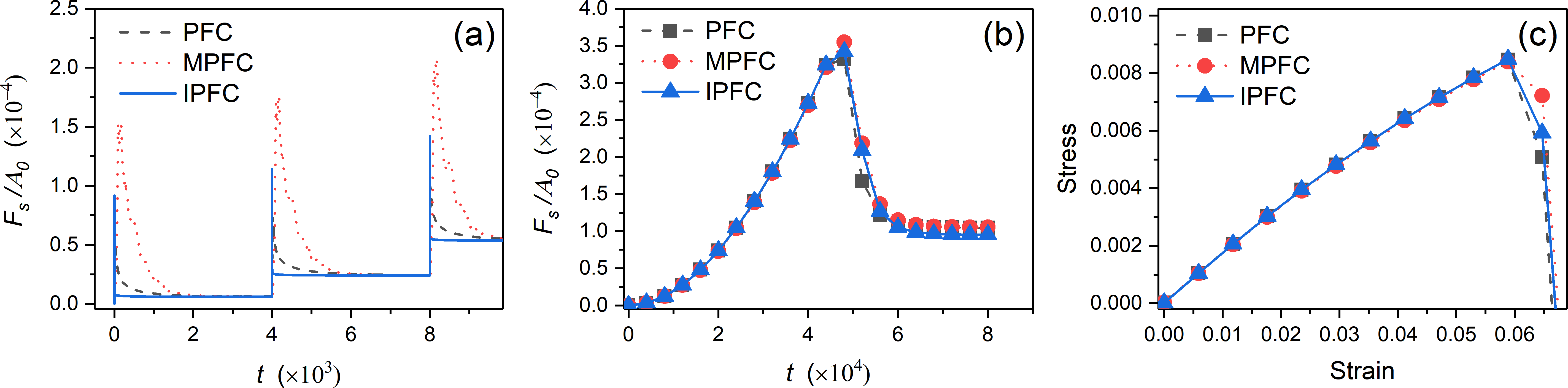
Figure 3: Mechanical behavior of the double notched nanoribbon calculated via three different methods, for a system grid size $256\times 512$ (with $\mathcal{A}_{0}=L_{x}^{0}\times L_{y}^{0}=196\Delta x\times 340\Delta y$) and strain rate $\dot{\varepsilon}=1.471\times 10^{-6}$. (a) Time evolution of strain energy density $F_{s}/\mathcal{A}_{0}$ during the first three steps of stretching, where the end state of each stretching step after mechanical relaxation is used to evaluate the mechanical property of the system in (b) and (c). (b) Strain energy density $F_{s}/\mathcal{A}_{0}$ evaluated at the mechanically relaxed state as a function of time. (c) Stress-strain relation. In (a) and (b), a factor of $\alpha^{2}/\beta$ has been scaled for time $t$ in MPFC results.

The time evolution of mechanically relaxed strain energy density are given in Fig. 3(b), which is used to calculate the stress-strain curves in Fig. 3(c) based on Eq. (9). Very similar stress-strain relation is obtained for all three methods, particularly in the elastic regime, although there are some small differences around the fracture stage. A behavior of brittle fracture is observed in our simulations [see Fig. 3(c)], which is qualitatively similar to the MD simulation results for pristine Zhao et al. (2009); Zhao and Aluru (2010) or grain boundary Grantab et al. (2010) samples of graphene.

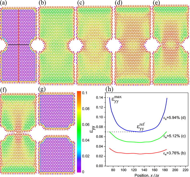
Figure 4: Spatial distribution of strain $\varepsilon_{yy}$ over the double notched nanoribbon simulated in Fig. 3 using the IPFC scheme, at $\varepsilon_{e}=0$, $3.76\%$, $5.12\%$, $5.94\%$, $6.82\%$, $7.18\%$, and $9.24\%$ from (a) to (g). (h) Plots of $\epsilon_{yy}$ along the central horizontal line of the nanoribbon [black line in (a)] at different strain levels.

The spatial distribution of strain $\varepsilon_{yy}=\partial u_{y}/\partial y$ in the double notched sample is presented in Fig. 4, with results obtained from IPFC simulation at different stages of imposed tension. A numerical image processing technique, the Peak Pairs algorithm Galindo et al. (2007); Wang et al. (2015), is used to calculate the local strain $\varepsilon_{yy}$. Before the fracture occurs, the strain is concentrated around the notch roots, as seen in Figs. 4(a)–4(d). This can be quantified by the stress-concentration factor $K_{t}$ measuring the ratio between the maximum stress $\sigma^{\rm max}_{yy}$ at the notch root and the net-section stress $\sigma^{\rm net}_{yy}$ Baratta and Neal (1970). In PFC it is approximated by $K_{t}=\sigma^{\rm max}_{yy}/\sigma^{\rm net}_{yy}\approx\varepsilon^{\rm max}_{yy}/\varepsilon^{\rm ref}_{yy}$ through an estimate from linear elasticity Stefanovic et al. (2006), where $\varepsilon^{\rm max}_{yy}$ and $\varepsilon^{\rm ref}_{yy}$ are indicated in Fig. 4(h) showing the cross-section profile of strain distribution in between the notches. Our IPFC simulation gives $K_{t}=1.991$, well agreeing with the value of $2.012$ calculated from the empirical formula Baratta and Neal (1970) $K_{t}=(0.78+2.243\sqrt{L/R})[0.993+0.18(2L/W)-1.06(2L/W)^{2}+1.71(2L/W)^{3}](1-2L/W)$, where $W=21a_{0}$ and $L=R=3.5a_{0}$ in our setup (see Fig. 1). Similar quantitative agreement has also been found in the previous MPFC study Stefanovic et al. (2006). As the sample is further stretched, cracks are initiated at the tips of two notches with concentrated stresses and propagate inside horizontally, as expected, causing the fracture of the nanoribbon. The locations of the strain concentration propagate accordingly, as illustrated in Figs. 4(e)–4(g).

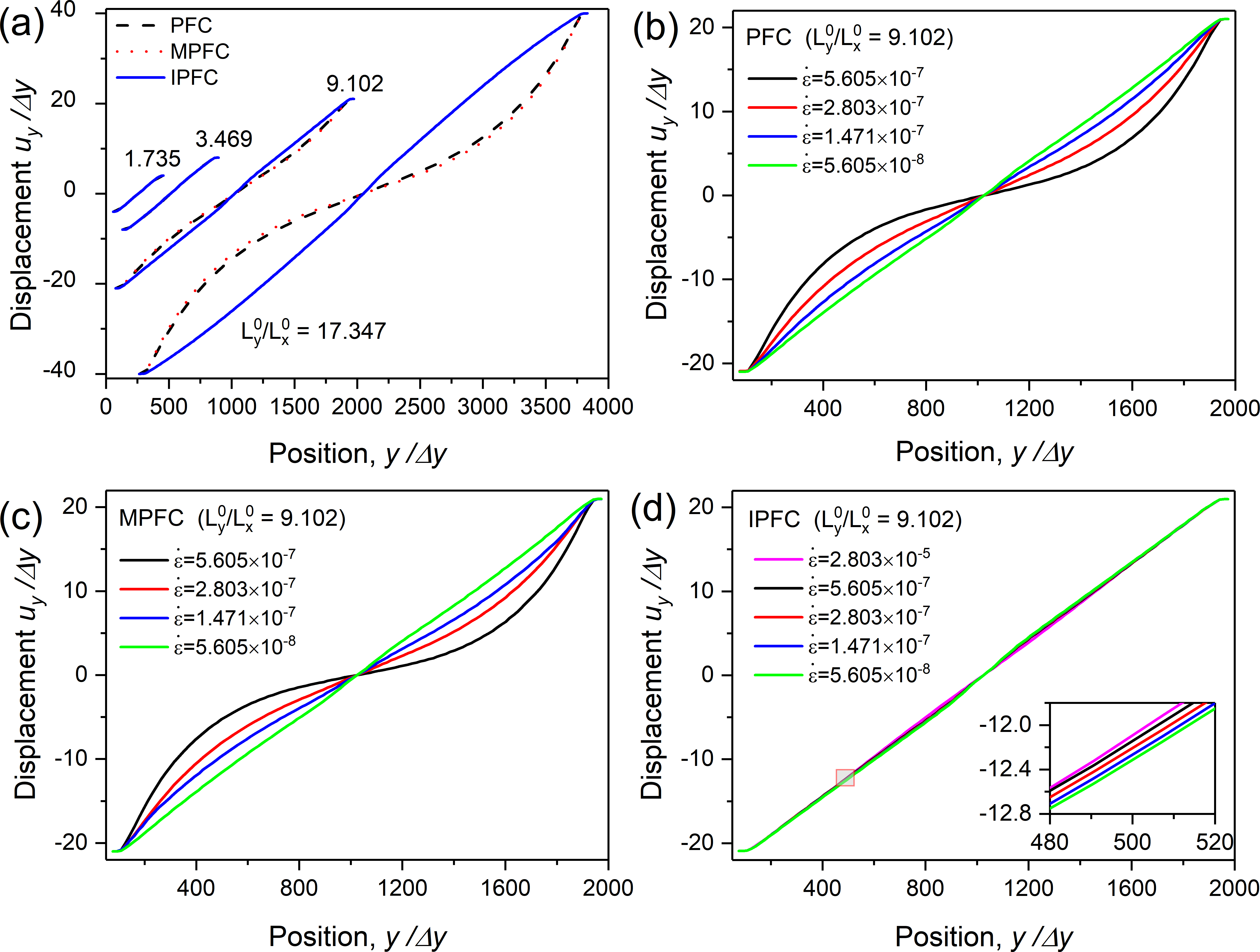
Figure 5: The displacement $u_{y}$ along the tensile loading direction in the middle of the double notched nanoribbon simulated [e.g., the red vertical line in Fig. 4(a)], at strain $\varepsilon_{e}=2.35\%$. (a) The displacements in systems of different aspect ratios simulated by PFC, MPFC, and IPFC methods, for $L_{y}^{0}/L_{x}^{0}=1.735$ (with system size $256\Delta x\times 512\Delta y$), $L_{y}^{0}/L_{x}^{0}=3.469$ (system size $256\Delta x\times 1024\Delta y$), $L_{y}^{0}/L_{x}^{0}=9.102$ (system size $256\Delta x\times 2048\Delta y$), and $L_{y}^{0}/L_{x}^{0}=17.347$ (system size $256\Delta x\times 4096\Delta y$). In these systems $L_{x}^{0}=196\Delta x$ and $\dot{\varepsilon}=1.471\times 10^{-7}$ are kept the same. In (b), (c), and (d) the double notched sample with $L_{y}^{0}/L_{x}^{0}=9.102$ is simulated under different applied strain rates, by using PFC, MPFC, and IPFC schemes, respectively.

It is important to note that while results from these three methods show similarities at small system size and strain rate, they deviate more from each other at larger length and/or faster rate of stretching. This can be seen clearly in Fig. 5 which shows the elastic response of the nanoribbon with different initial vertical length $L_{y}^{0}$ (while $L_{x}^{0}$ is kept unchanged) or different applied strain rate $\dot{\varepsilon}$ under tensile deformation. For a system with total grid size $256\times 512$ and $L_{y}^{0}/L_{x}^{0}=340/196=1.735$ (as studied in Figs. 3 and 4), at small strain the 1D profile of the displacement field $u_{y}$ exhibits the same linear spatial dependence along the middle vertical line of the nanoribbon for PFC, MPFC, and IPFC results, as shown in Fig. 5(a). A similar behavior applies to larger size $256\times 1024$ with $L_{y}^{0}/L_{x}^{0}=3.469$. However, when $L_{y}^{0}$ is further increased (e.g., for grid size $256\times 2048$ with $L_{y}^{0}/L_{x}^{0}=9.102$, and $256\times 4096$ with $L_{y}^{0}/L_{x}^{0}=17.347$), at the same strain rate $\dot{\varepsilon}=1.471\times 10^{-7}$ a deviation from the linear distribution of $u_{y}$ occurs for both the original PFC model due to its slow, diffusive dynamics of relaxation, and the MPFC model as its elastic interaction length has been exceeded at such a large length scale.

Similar effects can be found in terms of increasing strain rate $\dot{\varepsilon}$. For both PFC and MPFC results given in Figs. 5(b) and 5(c) at $L_{y}^{0}/L_{x}^{0}=9.102$, it is shown that the fully mechanically relaxed state can always be approached as long as the strain rate is sufficiently small (at the order of $10^{-8}$ or less; i.e., if waiting for long enough time within each stretching step) which, however, is computationally expensive particularly for large systems. At faster but more realistic strain rates, a viscoelastic behavior of the displacement field is obtained, instead of the elastic response, since the stressed system dominated by diffusive processes (or with inadequate elastic relaxation mechanism) needs long enough time to equilibrate elastically. Although in MPFC one can adjust $\alpha$ and $\beta$ parameter values to reach larger length and time scales of elastic interaction, too large $\alpha$ and/or too small $\beta$ would cause the difficulty of numerical convergence (e.g., needing very small $\Delta t$) and reduce the computational efficiency. In addition, it has been shown that there exists a lower limit of the dissipative parameter $\beta$; below this limit no faster relaxation dynamics can be gained Heinonen et al. (2016a).

In contrast, such restrictions of system size and strain rate are significantly released for IPFC given its interpolation scheme, which instead can always lead to elastic equilibrium of the system within a short time scale for all the system sizes [see Fig. 5(a)] and strain rates [see Fig. 5(d)] examined in our tests. Our calculations show that the IPFC scheme is at least an order of magnitude more efficient than the original PFC and MPFC methods, giving a clear advantage of IPFC for the study of mechanical deformation and response of solid systems.

III.1.2 Deformation process during tensile test and fracture

To further investigate the detailed process of elastic deformation and fracture in the uniaxially stressed nanoribbon, a system of long enough length along the pulling direction with $L_{y}^{0}/L_{x}^{0}=1784/196=9.102$ (and grid size $256\times 2048$) is simulated at the same moderate strain rate $\dot{\varepsilon}=5.605\times 10^{-7}$ using three PFC methods. The calculated results of stress-strain relation are given in Fig. 6, showing the discrepancies of mechanical property identified from original PFC, MPFC, and IPFC in this large system. This is different from the small-system similarity presented in Fig. 3. The discrepancies occur even in the early stage of small-strain elastic regime (for which only IPFC yields the expected linear elastic behavior), which can be attributed to different speeds of elastic relaxation in different methods and the elastic vs viscoelastic behavior of the displacement field (see Fig. 5). In addition, different values of fracture strain and strength are obtained through three methods.

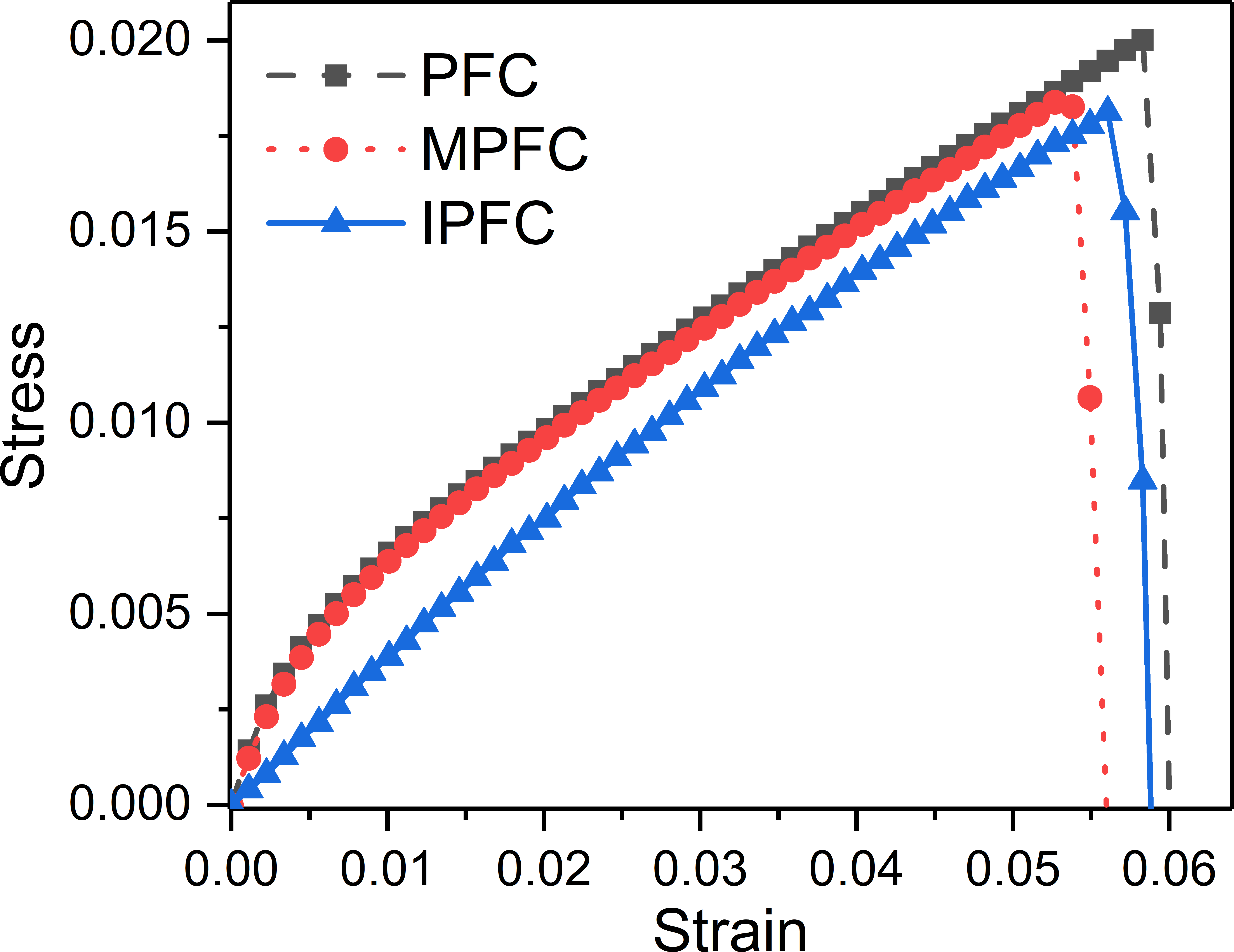
Figure 6: Stress-strain curves obtained from three different methods, for $L_{y}^{0}/L_{x}^{0}=9.102$ and $\dot{\varepsilon}=5.605\times 10^{-7}$.

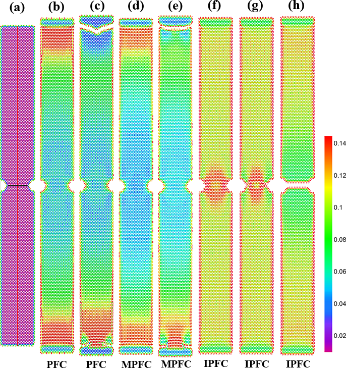
Figure 7: Spatial distribution of strain $\varepsilon_{yy}$ over the double notched nanoribbon simulated in Fig. 6, at (a) $\varepsilon_{e}=0$, (b) $4.98\%$ and (c) $6.32\%$ using PFC, (d) $5.02\%$ and (e) $5.89\%$ using MPFC, and (f) $5.45\%$, (g) $5.54\%$, and (h) $6.57\%$ using IPFC scheme.

The corresponding results of color-coded spatial distribution of strain $\varepsilon_{yy}$ are illustrated in Fig. 7. In the case of original PFC model, the strain and stress first concentrate in the vicinity of the traction regions and then propagate into the internal of the sheet, but only partially due to the slow elastic propagation [see Fig. 7(b)]. This causes the over-concentrating of stress around the boundary with the loading region which exceeds that of the notches, leading to the cracking near the edges of the traction regions [Fig. 7(c)] instead of the notch roots. This abnormal fracture behavior also occurs in the MPFC simulation given its limited range of elastic interaction, as shown in Figs. 7(d) and 7(e). In comparison, Figs. 7(f)–7(h) show that as a result of fast elastic relaxation in IPFC, the strain distributes across the whole sheet and concentrates around the notch tips, initializing the crack formation there and causing the subsequent brittle cleavage fracture as expected in real materials.

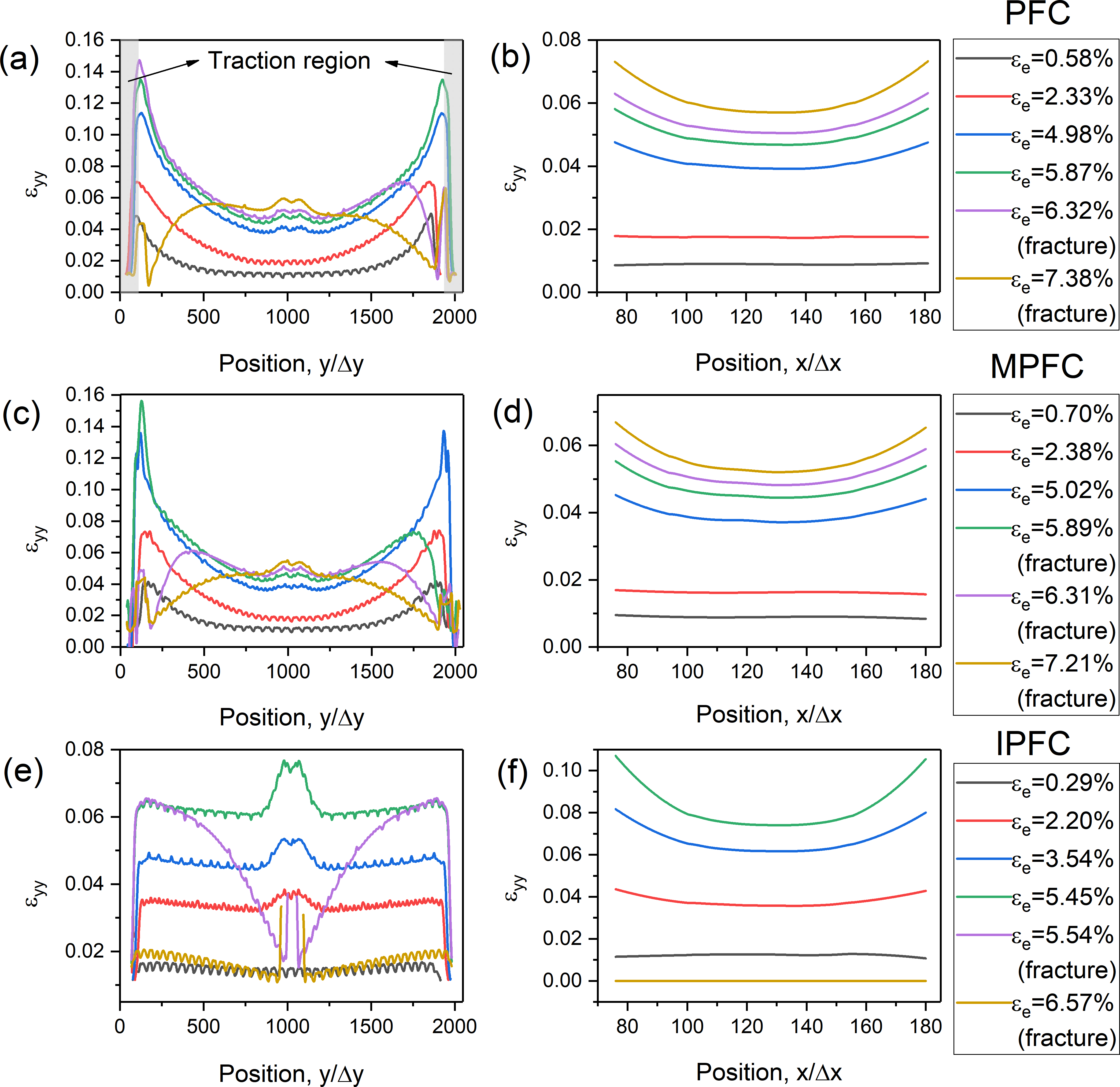
Figure 8: Plots of $\epsilon_{yy}$ at different applied strain levels, either along the tensile loading direction in the middle of nanoribbon [the red vertical line in Fig. 7(a)] for (a), (c), (e), or perpendicular to the loading direction [the black central horizontal line in Fig. 7(a)] for (b), (d), (f).

These two different scenarios of fracture process can be further analyzed from the evolution of 1D cross-section profiles of strain distribution plotted in Fig. 8, either along the vertical pulling direction at $x=L_{x}/2$ [i.e., $\varepsilon_{yy}$ vs $y$ in Fig. 8 (a), (c), (e)], or perpendicular to the pulling at $y=L_{y}/2$ [i.e., $\varepsilon_{yy}$ vs $x$ in Fig. 8 (b), (d), (f)]. Comparing the results between three methods clearly shows how the discrepancy emerges among PFC, MPFC, and IPFC schemes due to different strain propagation processes. For the $y$-direction profiles given in Figs. 8(a) and 8(c) for PFC and MPFC, although the strain inside the traction regions is very small, consistent with our traction boundary condition setup, the maxima of local strain always occur near the boundary between active and traction regions before fracture (with $\varepsilon_{e}$ up to 5.87% for PFC and 5.05% for MPFC in the figures), which can even reach a value close to 14% for $\varepsilon_{yy}$. This contradicts the usual expectation of stress concentration around the notch region located in the middle of the nanoribbon (which instead shows close-to-minimum strain). It indicates an outcome of inadequate mechanical relaxation in these two methods which requires a much longer time for the propagation of the imposed strain and stress into the internal of this large system. Such large strains concentrated at the active-traction boundaries eventually lead to the cracking and fracture there, showing as a rapid decrease of strain values at the crack locations [see strain profiles of $\varepsilon_{e}=6.32\%$ (purple) and 7.38% (yellow) in Fig. 8(a) for PFC, and 5.89% (green), 6.31% (purple), and 7.21% (yellow) in Fig. 8(c) for MPFC].

A qualitatively different behavior is observed in the results of IPFC. As shown in Fig. 8(e), within each stretching step the stress applied at the boundaries has well propagated into the bulk, and before the occurrence of fracture the strain distribution peaks around the middle ($y=L_{y}/2$) where the notch section is located, demonstrating the efficiency of IPFC scheme in terms of fast elastic relaxation when subjected to mechanical deformation. Within the notch section the strain is concentrated at the roots as expected, i.e., at the two ends of the $x$-direction profiles given in Fig. 8(f). The corresponding stress-concentration factor $K_{t}$, which can be approximated as the ratio between maximum and minimum values of $\varepsilon_{yy}$ along the $\varepsilon_{yy}$ vs $x$ profile, is larger than that of PFC and MPFC plots shown in Figs. 8(b) and 8(d). Cracks are then initialized at the notch tips and the brittle fracture occurs, which is associated with the steep drop of strain in the middle notch region of Fig. 8(e) and the zero strain value across the central notch section in Fig. 8(f) when $\varepsilon_{e}=5.54\%$ (purple) and 6.57% (yellow).

III.2 Temperature and chirality dependence of mechanical property

Given the efficiency of the IPFC scheme as demonstrated above, we use it to systematically examine the mechanical property of the double notched nanoribbon with honeycomb lattice structure, particularly effects of system temperature and chirality. Noting that the PFC free energy functional Eq. (1) with honeycomb symmetry has been used as an effective approach for the study of 2D graphene monolayers Elder et al. (2016); Smirman et al. (2017), our calculations are expected to reveal some important mechanical properties of graphene.

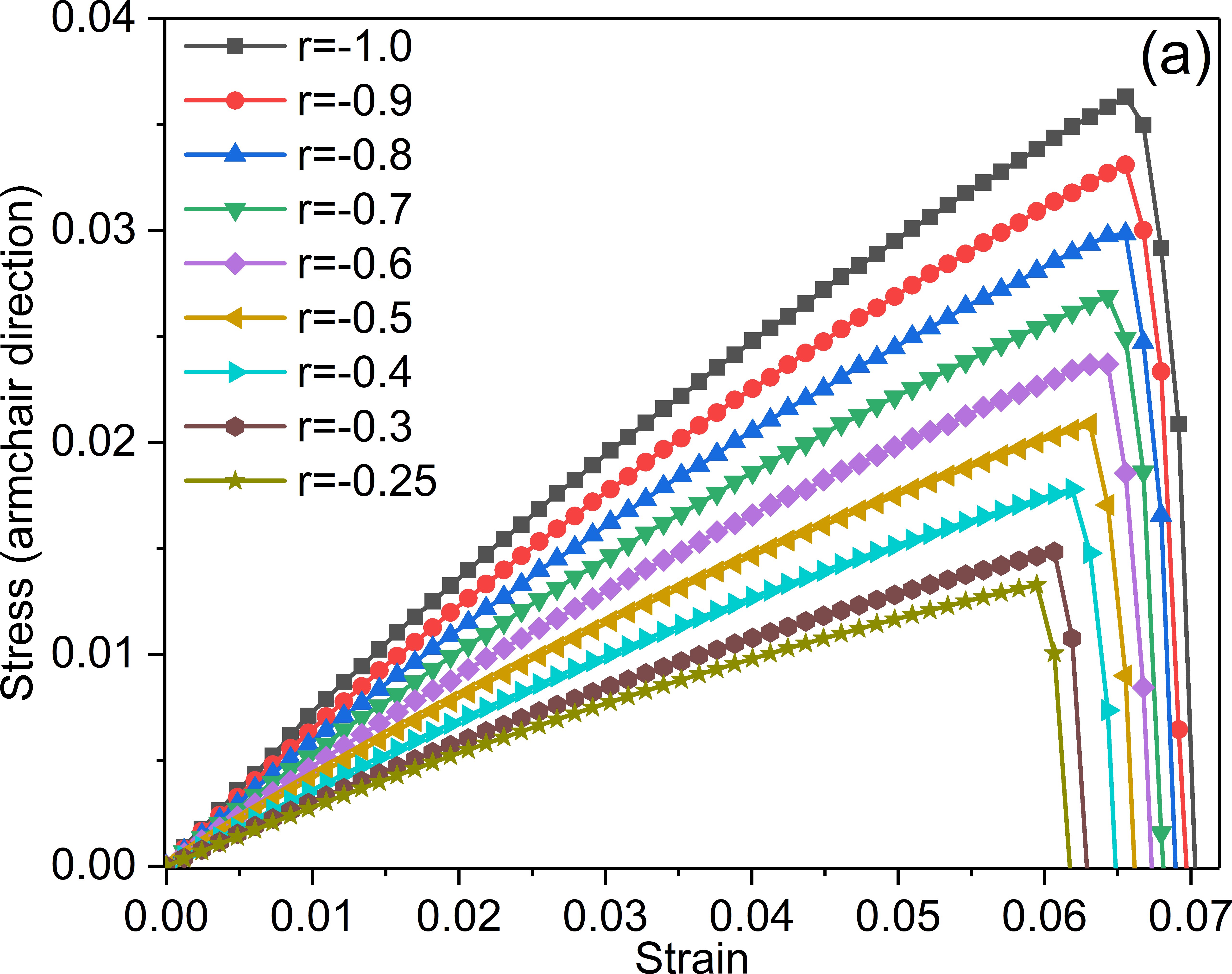
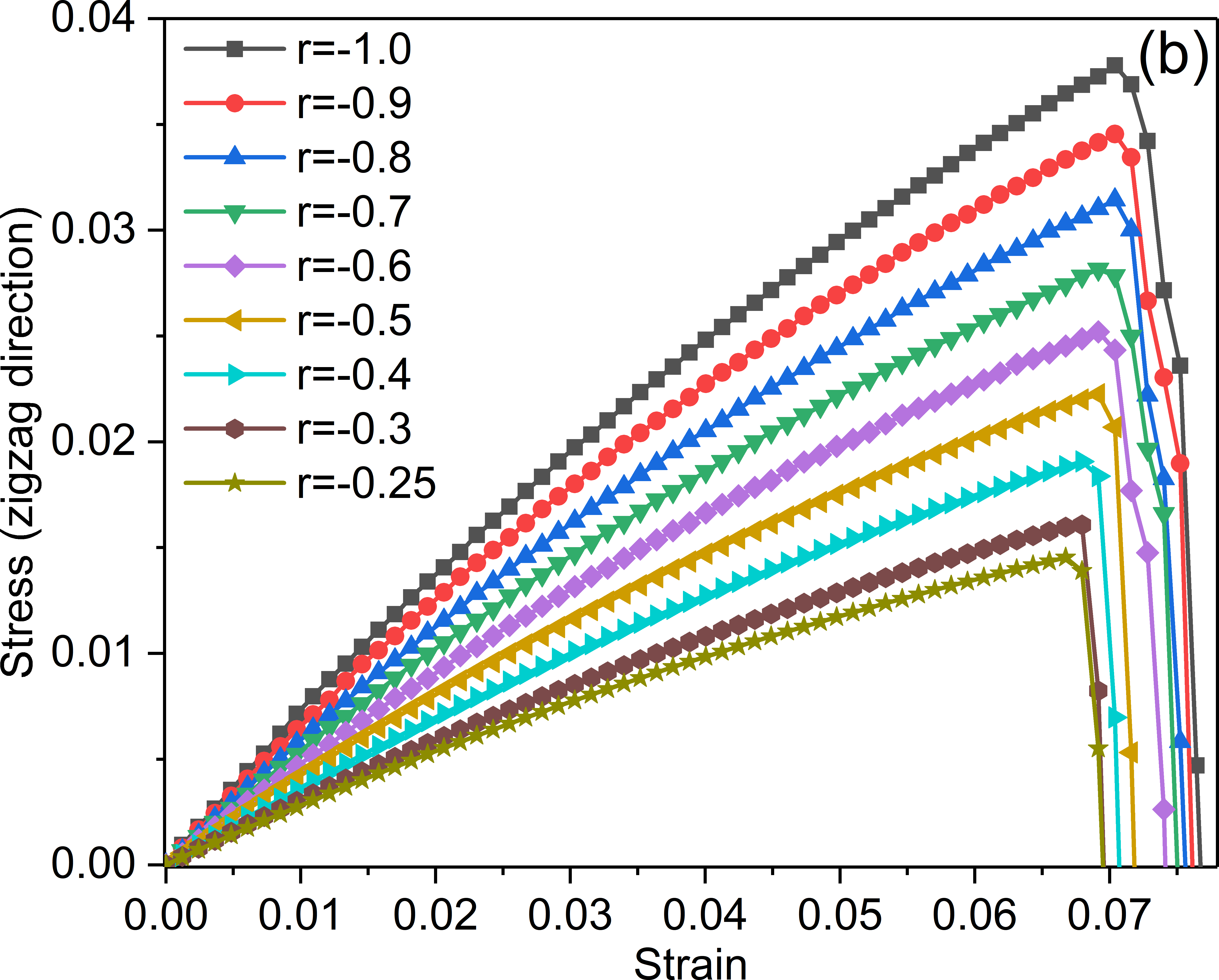
Figure 9: Temperature-dependent stress-strain relation at different values of temperature parameter $r$, for the double notched nanoribbon system under uniaxial tension along the armchair (a) and zigzag (b) directions. In each simulation the total system size is $256\Delta x\times 2048\Delta y$, with $L_{y}^{0}/L_{x}^{0}=8.408$, and the applied strain rate is $\dot{\varepsilon}=6.068\times 10^{-7}$.

All the results given above are for the uniaxial tension along the armchair direction of honeycomb structure (see Fig. 1) at a fixed temperature parameter value $r=-0.5$. More general results of stress-strain relation are presented in Fig. 9, as obtained from IPFC simulations for stretching along both armchair and zigzag directions at various temperatures. Note that the temperature parameter $r$ is related to the distance from the melting point, and greater value of $r$ corresponds to higher temperature. In our simulations its largest value (i.e., $r=-0.25$) is chosen such that the double notched nanoribbon can still maintain its faceted surface configuration during the mechanical deformation. Results across different temperatures (i.e., different $r$ values) give qualitatively similar behaviors of mechanical response and brittle fracture, as shown in Figs. 9(a) and 9(b) for uniaxial tensile tests along the armchair and zigzag directions, respectively, although the quantitative outcomes are different in both linear and nonlinear elastic and fracture regimes.

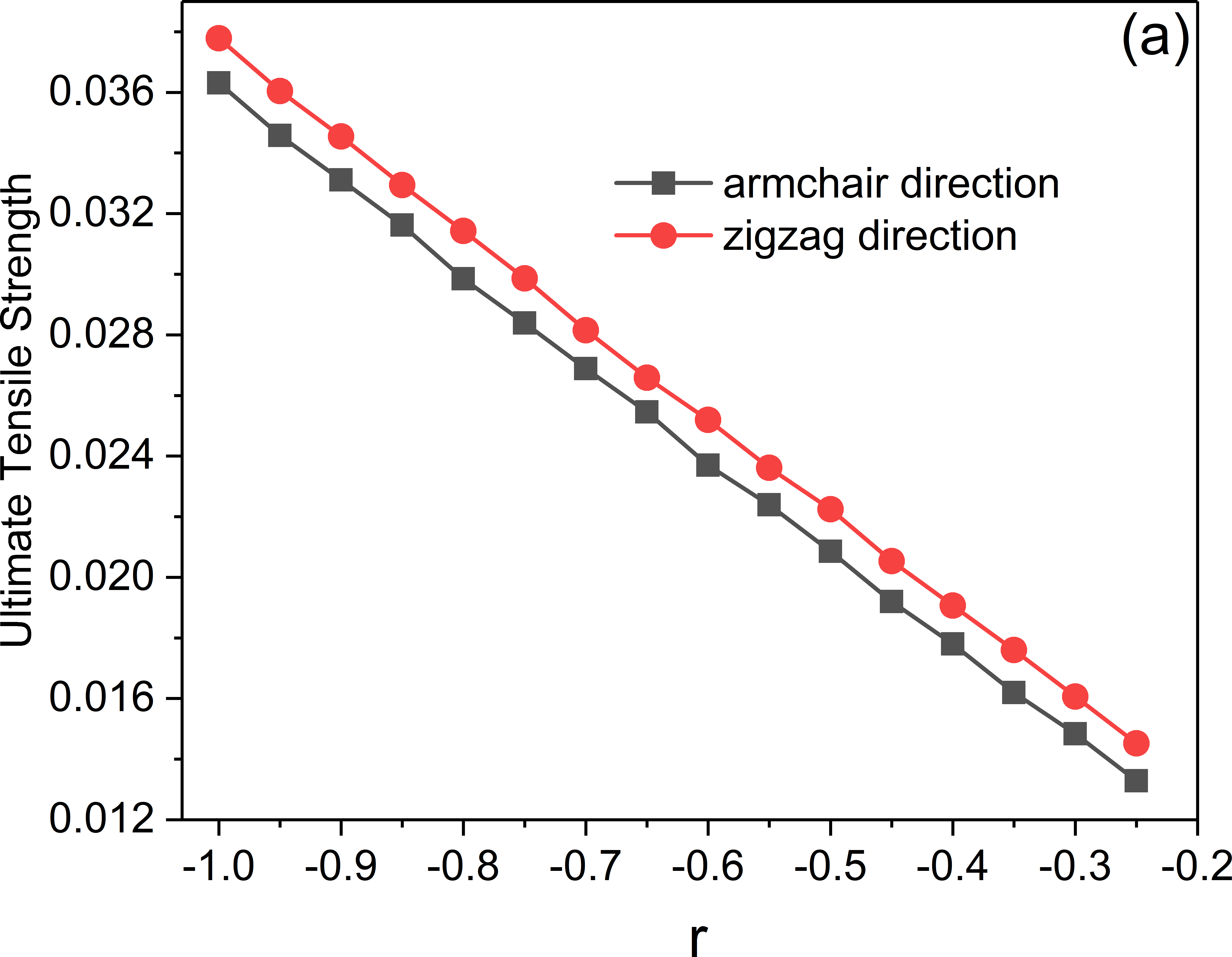
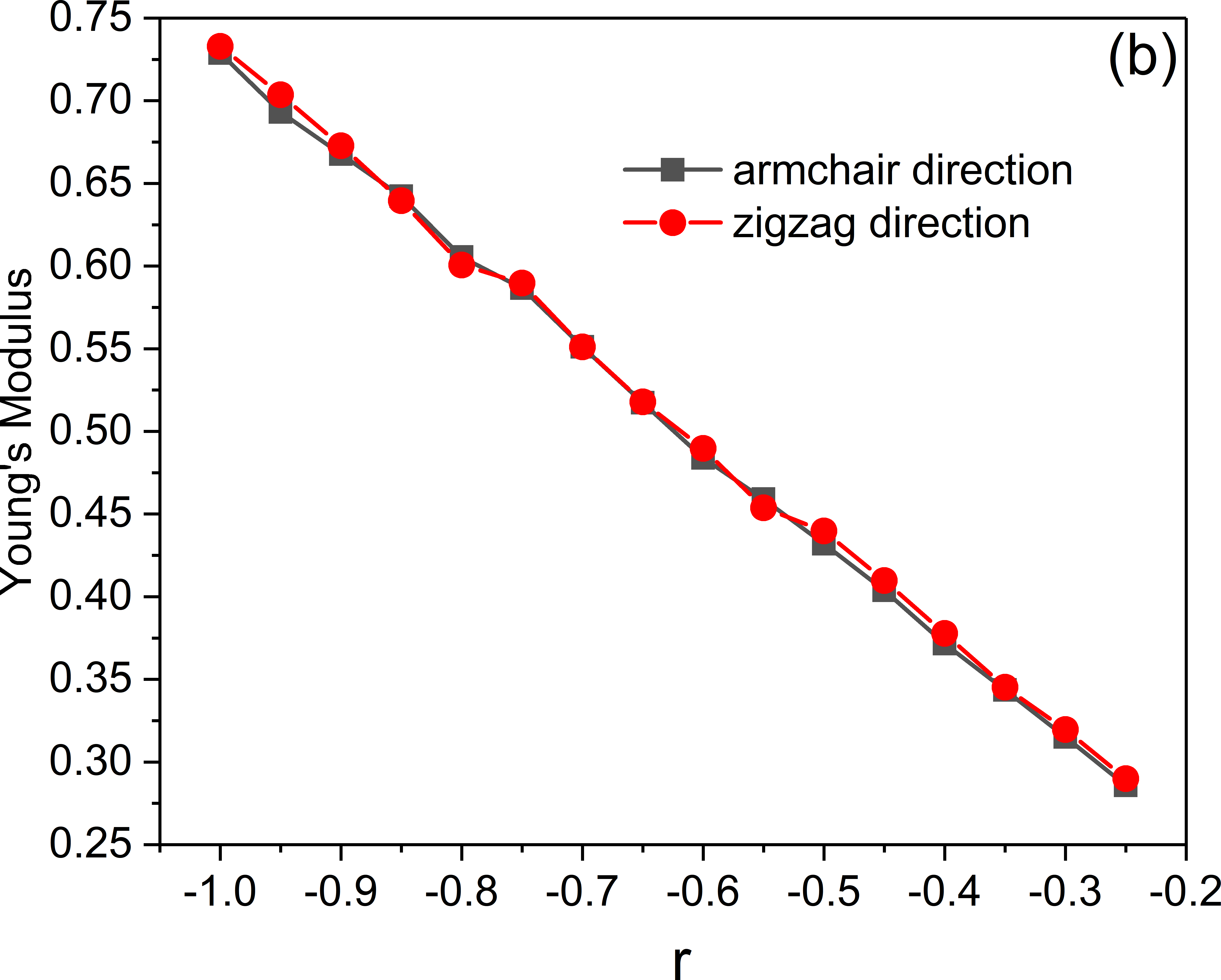
Figure 10: (a) Ultimate tensile strength as a function of temperature parameter $r$. (b) Young’s modulus as a function of $r$. The results are determined from the stress-strain relation given in Fig. 9.

The corresponding values of temperature-varying ultimate tensile strength and Young’s modulus are presented in Fig. 10. The ultimate strength is identified as the value of maximum stress before fracture, while the Young’s modulus, $Y=(\partial\sigma_{e}/\partial\varepsilon_{e})_{\varepsilon_{e}\rightarrow 0}$, is calculated from the linear elasticity regime of the stress-strain curve at small strains (i.e., the slope of the stress-strain line for $\varepsilon_{e}<0.5\%$). Fig. 10(a) shows the decrease of the ultimate strength with increasing temperature (i.e., increasing $r$), which is consistent with the previous MD results for bulk pristine graphene simulated across a broad range of temperatures Zhao and Aluru (2010). The similar temperature weakening behavior is also obtained for Young’s modulus [see Fig. 10(b)]. This can be attributed to the weakened interparticle interaction strength and hence the softening of crystal at higher temperature, as found in recent MD Zhao and Aluru (2010) and MC Zakharchenko et al. (2009) calculations which showed the decrease of Young’s modulus of graphene at high enough temperatures.

Figure 10(a) also indicates slightly higher ultimate strengths in the zigzag direction as compared to the armchair direction across the whole temperature range simulated, a result of chirality effect that is consistent with the findings in both MD Zhao et al. (2009) and ab initio DFT Liu et al. (2007) calculations of pristine graphene. A different behavior is given in Fig. 10(b) for Young’s modulus, showing very close values along the armchair and zigzag directions. It is different from the MD result of graphene nanoribbons Zhao et al. (2009) which yielded higher Young’s modulus along the zigzag direction than the armchair one. This discrepancy can be understood from the fact that the out-of-plane deformations have been incorporated in the MD simulation of free-standing graphene sheets, but are neglected in our PFC simulations which are restricted to purely 2D planar structures. Under large degree of lateral stretching (particularly close to fracture with high tensile strain) the stretched sheet would be flattened and any initial out-of-plane variations would then play a negligible role, resulting in the consistency between 3D MD and 2D IPFC results for the chirality dependence of ultimate strength. However, at very small strains used to calculate Young’s modulus, these variations would influence the evaluation of elastic properties, as seen in the discrepancy described above. This is also consistent with the previous atomistic study of graphene Zhao et al. (2009), which showed that the purely 2D tight-binding calculations yielded close magnitudes of Young’s modulus for armchair and zigzag directions, similar to our 2D IPFC results but different from those of 3D MD calculations involving out-of-plane effects.

IV Conclusions

We have developed a computational method to effectively simulate the processes of mechanical relaxation and fracture in PFC, by applying an interpolation scheme on the PFC density field based on an imposed condition for the displacement field to ensure local elastic equilibration and fast global mechanical relaxation. This IPFC method is applied to the simulation of a sample 2D system with honeycomb lattice structure under uniaxial tension. The results are compared to those obtained by original PFC and MPFC simulations and to previous MD, MC, and ab initio DFT calculations of graphene. The IPFC-calculated stress-strain relation, ultimate strength of brittle fracture and Young’s modulus are qualitatively consistent with those of atomistic simulations Zhao et al. (2009); Zhao and Aluru (2010); Liu et al. (2007); Zakharchenko et al. (2009), in terms of effects of system temperature (for both ultimate strength and Young’s modulus) and chirality (armchair vs zigzag direction, for ultimate strength and also Young’s modulus of 2D calculations). The outcomes demonstrate a much more efficient process of dynamic relaxation and mechanical equilibration for IPFC scheme, in comparison to the original PFC and MPFC methods. Although the use of this interpolation scheme is still subjected to the scales of conventional PFC-type simulations, its advantage applies particularly to the scenarios with large enough system sizes and/or high enough strain rates, where the original PFC and MPFC models would generate qualitatively incorrect results of mechanical response due to their inadequate mechanisms for strain propagation and mechanical relaxation, including the stress-strain relation, spatial distribution of strain or stress, spatial dependence of the displacement field even in the linear elastic regime, and the fracture behavior.

It is noted that although this IPFC numerical scheme bears some similarity of treatment as compared to a recently developed mechanically-equilibrated amplitude model Heinonen et al. (2014) in terms of imposing extra constraints on PFC dynamics, the detailed setup of constraints is very different and the algorithm developed here is mainly for the study of mechanical deformation and fracture. In the amplitude model Heinonen et al. (2014) the equilibrium condition was imposed only on the phases of amplitudes, while in our IPFC scheme the interpolation is applied to the whole density field (equivalent to both magnitudes and phases). Importantly, our method is applied to the full model of PFC instead of the amplitude expansion at slow scales, so that the key features of original PFC model are maintained, particularly the coupling between microscopic and mesoscopic length scales Huang (2013) and the resulting effects of lattice pinning and Peierls barriers for dislocation defects that are missing in the amplitude expansion but important for examining the mechanical response of materials. Even when directly applying this IPFC scheme to the amplitude equations (which would be straightforward), the interpolation would be imposed on both the average density $\phi_{0}$ and the full complex amplitudes $A_{nm}$ but not only on their phases. Note also that the interpolation algorithm [Eqs. (16) and (17)] used here for uniaxial tensile test can be extended straightforwardly to the study of compressive test as well as biaxial tension/compression of materials. In addition, this IPFC scheme is independent of the model free energy adopted and thus can be directly used for any other PFC models with more complex free energy functionals (see, e.g., Refs. Greenwood et al. (2010); Mkhonta et al. (2013); Wang et al. (2018); Taha et al. (2017)) for the modeling of a wider variety of material systems with different crystalline symmetries and microstructures.

*

Appendix A Numerical method for solving MPFC equation

In the following we outline the derivation of a pseudospectral algorithm for solving the MPFC dynamic equation (7). We follow the method of Ref. Chandrasekhar (1943) for the formal solution of an ordinary differential equation (now in Fourier space) with second-order time derivative, as adopted in Ref. Adland et al. (2013). Compared to the explicit numerical scheme derived in Ref. Adland et al. (2013) for MPFC, here we (i) express the equations of algorithm in terms of real quantities (using hyperbolic functions), and (ii) use an implicit treatment for nonlinear terms and the predictor-corrector method Cross et al. (1994).

In Fourier space the MPFC equation (7) is written as

$$\frac{\partial^{2}\hat{\phi}_{\vec{q}}}{\partial t^{2}}+\beta\frac{\partial\hat{\phi}_{\vec{q}}}{\partial t}=\sigma_{q}\hat{\phi}_{\vec{q}}+\hat{N}_{\vec{q}},$$ (18)

where $\hat{\phi}_{\vec{q}}$ is the Fourier component of the density field $\phi$, $\sigma_{q}=-\alpha^{2}q^{2}[r+(1-q^{2})^{2}]$ with wave number $q$, and $\hat{N}_{\vec{q}}$ is the Fourier transform of the nonlinear terms $\alpha^{2}\nabla^{2}(\tau\phi^{2}+\phi^{3})$. The general solution of Eq. (18) is of the form

$$\hat{\phi}_{\vec{q}}=a_{1}(t)e^{\frac{1}{2}(-\beta+\beta_{1})t}+a_{2}(t)e^{\frac{1}{2}(-\beta-\beta_{1})t},$$ (19)

where $\beta_{1}=\sqrt{\beta^{2}+4\sigma_{q}}$, and $a_{1}$ and $a_{2}$ satisfy the condition Chandrasekhar (1943) $(da_{1}/dt)\exp[\frac{1}{2}(-\beta+\beta_{1})t]+(da_{2}/dt)\exp[\frac{1}{2}(-\beta-\beta_{1})t]=0$, such that

$$\frac{da_{1}}{dt}e^{\beta_{1}t}+\frac{da_{2}}{dt}=0.$$ (20)

Substituting Eq. (19) into Eq. (18) and combining with Eq. (20), we get

$$\frac{da_{1}}{dt}=\frac{1}{\beta_{1}}\hat{N}_{\vec{q}}(t)e^{\frac{1}{2}(\beta-\beta_{1})t},$$ (21)

$$\frac{da_{2}}{dt}=-\frac{1}{\beta_{1}}\hat{N}_{\vec{q}}(t)e^{\frac{1}{2}(\beta+\beta_{1})t}.$$ (22)

Integrating them from $t$ to $t+\Delta t$ gives

$$a_{1}(t+\Delta t) = \frac{1}{\beta_{1}}\int_{t}^{t+\Delta t}dt^{\prime}e^{\frac{1}{2}(\beta-\beta_{1})t^{\prime}}\hat{N}_{\vec{q}}(t^{\prime})+a_{1}(t),~{}~{}\quad$$ (23)

$$a_{2}(t+\Delta t) = -\frac{1}{\beta_{1}}\int_{t}^{t+\Delta t}dt^{\prime}e^{\frac{1}{2}(\beta+\beta_{1})t^{\prime}}\hat{N}_{\vec{q}}(t^{\prime})+a_{2}(t).~{}~{}\quad$$ (24)

For a given time $t$, $a_{1}(t)$ and $a_{2}(t)$ can be expressed in terms of $\hat{\phi}_{\vec{q}}$ and its time derivative $\hat{u}_{\vec{q}}$, which is determined from Eqs. (19) and (20) to be

$$\hat{u}_{\vec{q}}(t)=\frac{\partial\hat{\phi}_{\vec{q}}}{\partial t} = \frac{1}{2}(-\beta+\beta_{1})a_{1}(t)e^{\frac{1}{2}(-\beta+\beta_{1})t}$$ (25)

$$- \frac{1}{2}(\beta+\beta_{1})a_{2}(t)e^{-\frac{1}{2}(\beta+\beta_{1})t}.$$

Combining Eqs. (19) and (25) leads to

$$a_{1}(t)=\frac{1}{\beta_{1}}e^{\frac{1}{2}(\beta-\beta_{1})t}\left[\hat{u}_{\vec{q}}(t)+\frac{1}{2}(\beta+\beta_{1})\hat{\phi}_{\vec{q}}(t)\right],$$ (26)

and

$$a_{2}(t)=-\frac{1}{\beta_{1}}e^{\frac{1}{2}(\beta+\beta_{1})t}\left[\hat{u}_{\vec{q}}(t)+\frac{1}{2}(\beta-\beta_{1})\hat{\phi}_{\vec{q}}(t)\right].$$ (27)

Evaluating Eqs. (19) and (25) at $t+\Delta t$ and using Eqs. (23) and (24) for $a_{1}(t+\Delta t)$ and $a_{2}(t+\Delta t)$, we have

$$\hat{\phi}_{\vec{q}}(t+\Delta t) = \frac{2}{\beta_{1}}\int_{t}^{t+\Delta t}dt^{\prime}e^{-\frac{1}{2}\beta(t+\Delta t-t^{\prime})}$$ (28)

$$\times\sinh\left[\frac{\beta_{1}}{2}(t+\Delta t-t^{\prime})\right]\hat{N}_{\vec{q}}(t^{\prime})$$

$$+ a_{1}(t)e^{-\frac{1}{2}(\beta-\beta_{1})(t+\Delta t)}$$

$$+ a_{2}(t)e^{-\frac{1}{2}(\beta+\beta_{1})(t+\Delta t)},$$

and

$$\hat{u}_{\vec{q}}(t+\Delta t) = \frac{1}{\beta_{1}}\int_{t}^{t+\Delta t}dt^{\prime}e^{-\frac{1}{2}\beta(t+\Delta t-t^{\prime})}$$ (29)

$$\times\left\{-\beta\sinh\left[\frac{\beta_{1}}{2}(t+\Delta t-t^{\prime})\right]\right.$$

$$\left.\quad+\beta_{1}\cosh\left[\frac{\beta_{1}}{2}(t+\Delta t-t^{\prime})\right]\right\}\hat{N}_{\vec{q}}(t^{\prime})$$

$$+ \frac{1}{2}(-\beta+\beta_{1})a_{1}(t)e^{\frac{1}{2}(-\beta+\beta_{1})(t+\Delta t)}$$

$$- \frac{1}{2}(\beta+\beta_{1})a_{2}(t)e^{-\frac{1}{2}(\beta+\beta_{1})(t+\Delta t)}.$$

For an implicit scheme, the nonlinear term $\hat{N}_{\vec{q}}(t^{\prime})$ is expanded to the first order as Cross et al. (1994)

$$\hat{N}_{\vec{q}}(t^{\prime})=\hat{N}_{\vec{q}}(t)+\frac{\hat{N}_{\vec{q}}(t+\Delta t)-\hat{N}_{\vec{q}}(t)}{\Delta t}(t^{\prime}-t).$$ (30)

Substituting Eq. (30) into Eqs. (28) and (29), integrating over $t^{\prime}$, and making use of Eqs. (26) and (27), we obtain the following numerical algorithm for solving the MPFC dynamic equation.

A.1 When $\sigma_{q}\neq 0$

If $\beta_{1}$ is real and positive (i.e., $\beta^{2}+4\sigma_{q}>0$), we have

$$\hat{\phi}_{\vec{q}}(t+\Delta t) = \hat{\phi}_{\vec{q}}(t)e^{-\frac{1}{2}\beta\Delta t}\left[\frac{\beta}{\beta_{1}}\sinh\left(\frac{1}{2}\beta_{1}\Delta t\right)+\cosh\left(\frac{1}{2}\beta_{1}\Delta t\right)\right]+\frac{2}{\beta_{1}}\hat{u}_{\vec{q}}e^{-\frac{1}{2}\beta\Delta t}\sinh\left(\frac{1}{2}\beta_{1}\Delta t\right)$$ (31)

$$+\frac{\hat{N}_{\vec{q}}(t)}{\sigma_{q}}\left\{e^{-\frac{1}{2}\beta\Delta t}\left[\frac{\beta}{\beta_{1}}\sinh\left(\frac{1}{2}\beta_{1}\Delta t\right)+\cosh\left(\frac{1}{2}\beta_{1}\Delta t\right)\right]-1\right\}$$

$$+\frac{\hat{N}_{\vec{q}}(t+\Delta t)-\hat{N}_{\vec{q}}(t)}{\sigma_{q}^{2}\Delta t}\left\{e^{-\frac{1}{2}\beta\Delta t}\left[\frac{\beta^{2}+\beta_{1}^{2}}{2\beta_{1}}\sinh\left(\frac{1}{2}\beta_{1}\Delta t\right)+\beta\cosh\left(\frac{1}{2}\beta_{1}\Delta t\right)\right]-\beta-\sigma_{q}\Delta t\right\},$$

and

$$\hat{u}_{\vec{q}}(t+\Delta t) = \frac{2\sigma_{q}}{\beta_{1}}\hat{\phi}_{\vec{q}}(t)e^{-\frac{1}{2}\beta\Delta t}\sinh\left(\frac{1}{2}\beta_{1}\Delta t\right)+\hat{u}_{\vec{q}}(t)e^{-\frac{1}{2}\beta\Delta t}\left[-\frac{\beta}{\beta_{1}}\sinh\left(\frac{1}{2}\beta_{1}\Delta t\right)+\cosh\left(\frac{1}{2}\beta_{1}\Delta t\right)\right]$$ (32)

$$+\frac{2\hat{N}_{\vec{q}}}{\beta_{1}}e^{-\frac{1}{2}\beta\Delta t}\sinh\left(\frac{1}{2}\beta_{1}\Delta t\right)$$

$$+\frac{\hat{N}_{\vec{q}}(t+\Delta t)-\hat{N}_{\vec{q}}(t)}{\sigma_{q}\Delta t}\left\{e^{-\frac{1}{2}\beta\Delta t}\left[\frac{\beta}{\beta_{1}}\sinh\left(\frac{1}{2}\beta_{1}\Delta t\right)+\cosh\left(\frac{1}{2}\beta_{1}\Delta t\right)\right]-1\right\}.$$

If $\beta_{1}=i\alpha_{1}$ is imaginary, i.e., $\beta^{2}+4\sigma_{q}<0$ and $\alpha_{1}=\sqrt{-(\beta^{2}+4\sigma_{q})}$, we only need to replace the terms $\frac{1}{\beta_{1}}\sinh(\frac{1}{2}\beta_{1}\Delta t)$ and $\cosh(\frac{1}{2}\beta_{1}\Delta t)$ in the above equations via

$$\frac{1}{\beta_{1}}\sinh\left(\frac{1}{2}\beta_{1}\Delta t\right)=\frac{1}{\alpha_{1}}\sin\left(\frac{1}{2}\alpha_{1}\Delta t\right),$$

$$\cosh\left(\frac{1}{2}\beta_{1}\Delta t\right)=\cos\left(\frac{1}{2}\alpha_{1}\Delta t\right).$$ (33)

In the case of $\beta_{1}=0$ (with $\beta^{2}+4\sigma_{q}=0$), those terms become

$$\frac{1}{\beta_{1}}\sinh\left(\frac{1}{2}\beta_{1}\Delta t\right)\rightarrow\frac{1}{2}\Delta t,\quad\cosh\left(\frac{1}{2}\beta_{1}\Delta t\right)=1.$$ (34)

A.2 When $\sigma_{q}=0$

In this case we have $\beta_{1}=\beta>0$, and thus Eqs. (31) and (32) are replaced by

$$\hat{\phi}_{\vec{q}}(t+\Delta t)=\hat{\phi}_{\vec{q}}(t)+\frac{1-e^{-\beta\Delta t}}{\beta}\hat{u}_{\vec{q}}(t)$$

$$+\hat{N}_{\vec{q}}(t)\left(\frac{\Delta t}{\beta}+\frac{e^{-\beta\Delta t}-1}{\beta^{2}}\right)$$

$$+\left[\hat{N}_{\vec{q}}(t+\Delta t)-\hat{N}_{\vec{q}}(t)\right]\left(\frac{\Delta t}{2\beta}-\frac{e^{-\beta\Delta t}-1+\beta\Delta t}{\beta^{3}\Delta t}\right),$$

(35)

$$\hat{u}_{\vec{q}}(t+\Delta t)=\hat{u}_{\vec{q}}(t)e^{-\beta\Delta t}-\hat{N}_{\vec{q}}(t)\frac{e^{-\beta\Delta t}-1}{\beta}$$

$$\qquad+\left[\hat{N}_{\vec{q}}(t+\Delta t)-\hat{N}_{\vec{q}}(t)\right]\frac{e^{-\beta\Delta t}-1+\beta\Delta t}{\beta^{2}\Delta t}.$$ (36)

To implement the implicit numerical scheme described above, we use the predictor-corrector method as in Ref. Cross et al. (1994). For the predictor step $\hat{N}_{\vec{q}}(t+\Delta t)-\hat{N}_{\vec{q}}(t)$ is assumed to be zero in Eqs. (31) and (32) or Eqs. (35) and (36), yielding the predictor or guess values of $\hat{\phi}_{\vec{q}}(t+\Delta t)$ and $\hat{u}_{\vec{q}}(t+\Delta t)$, while at the corrector step these guess values are used to evaluate $\hat{N}_{\vec{q}}(t+\Delta t)$ and thus the updated values of $\hat{\phi}_{\vec{q}}(t+\Delta t)$ and $\hat{u}_{\vec{q}}(t+\Delta t)$. At each time $t+\Delta t$, in principle the corrector step would include multiple iterations until the result reaches the desired numerical accuracy, although in our simulations we conduct only one predictor-corrector iteration which is sufficient for numerical convergence with enough accuracy of the outcomes.

References

- Lee et al. (2008) C. Lee, X. Wei, J. W. Kysar, and J. Hone, Science 321, 385 (2008).
- Zhao et al. (2009) H. Zhao, K. Min, and N. R. Aluru, Nano Lett. 9, 3012 (2009).
- Zhao and Aluru (2010) H. Zhao and N. R. Aluru, J. Appl. Phys. 108, 064321 (2010).
- Grantab et al. (2010) R. Grantab, V. B. Shenoy, and R. S. Ruoff, Science 330, 946 (2010).
- Liu et al. (2007) F. Liu, P. Ming, and J. Li, Phys. Rev. B 76, 064120 (2007).
- Zakharchenko et al. (2009) K. V. Zakharchenko, M. I. Katsnelson, and A. Fasolino, Phys. Rev. Lett. 102, 046808 (2009).
- Elder et al. (2002) K. R. Elder, M. Katakowski, M. Haataja, and M. Grant, Phys. Rev. Lett. 88, 245701 (2002).
- Elder and Grant (2004) K. R. Elder and M. Grant, Phys. Rev. E 70, 051605 (2004).
- Stefanovic et al. (2006) P. Stefanovic, M. Haataja, and N. Provatas, Phys. Rev. Lett. 96, 225504 (2006).
- Greenwood et al. (2010) M. Greenwood, N. Provatas, and J. Rottler, Phys. Rev. Lett. 105, 045702 (2010).
- Mkhonta et al. (2013) S. K. Mkhonta, K. R. Elder, and Z.-F. Huang, Phys. Rev. Lett. 111, 035501 (2013).
- Wang et al. (2018) Z.-L. Wang, Z. R. Liu, and Z.-F. Huang, Phys. Rev. B 97, 180102(R) (2018).
- Berry et al. (2006) J. Berry, M. Grant, and K. R. Elder, Phys. Rev. E 73, 031609 (2006).
- Taha et al. (2017) D. Taha, S. K. Mkhonta, K. R. Elder, and Z.-F. Huang, Phys. Rev. Lett. 118, 255501 (2017).
- Adland et al. (2013) A. Adland, A. Karma, R. Spatschek, D. Buta, and M. Asta, Phys. Rev. B 87, 024110 (2013).
- Salvalaglio et al. (2018) M. Salvalaglio, R. Backofen, K. R. Elder, and A. Voigt, Phys. Rev. Mater. 2, 053804 (2018).
- Skaugen et al. (2018a) A. Skaugen, L. Angheluta, and J. Viñals, Phys. Rev. B 97, 054113 (2018a).
- Wu and Voorhees (2012) K.-A. Wu and P. W. Voorhees, Acta Mater. 60, 407 (2012).
- Tóth et al. (2010) G. I. Tóth, G. Tegze, T. Pusztai, G. Tóth, and L. Granásy, J. Phys.: Condens. Matter 22, 364101 (2010).
- Guo et al. (2018) C. Guo, J. Wang, J. Li, Z. Wang, Y. Huang, J. Gu, and X. Lin, Acta Mater. 145, 175 (2018).
- Elder et al. (2016) K. R. Elder, Z. Chen, K. L. M. Elder, P. Hirvonen, S. K. Mkhonta, S.-C. Ying, E. Granato, Z.-F. Huang, and T. Ala-Nissila, J. Chem. Phys. 144, 174703 (2016).
- Smirman et al. (2017) M. Smirman, D. Taha, A. K. Singh, Z.-F. Huang, and K. R. Elder, Phys. Rev. B 95, 085407 (2017).
- Stefanovic et al. (2009) P. Stefanovic, M. Haataja, and N. Provatas, Phys. Rev. E 80, 046107 (2009).
- Zhou et al. (2017) W. Zhou, J. Wang, Z. Wang, Q. Zhang, C. Guo, J. Li, and Y. Guo, Comput. Mater. Sci. 127, 121 (2017).
- Gao et al. (2016) Y. Gao, Z. Luo, L. Huang, H. Mao, C. Huang, and K. Lin, Modelling Simul. Mater. Sci. Eng. 24, 055010 (2016).
- Hu et al. (2017) S. Hu, Z. Chen, W. Xi, and Y.-Y. Peng, J. Mater. Sci. 52, 5641 (2017).
- Heinonen et al. (2016a) V. Heinonen, C. V. Achim, and T. Ala-Nissila, Phys. Rev. E 93, 053003 (2016a).
- Majaniemi and Grant (2007) S. Majaniemi and M. Grant, Phys. Rev. B 75, 054301 (2007).
- Baskaran et al. (2016) A. Baskaran, Z. Guan, and J. Lowengrub, Comput. Methods Appl. Mech. Engrg. 299, 22 (2016).
- Tóth et al. (2014) G. I. Tóth, L. Gránásy, and G. Tegze, J. Phys.: Condens. Matter 26, 055001 (2014).
- Heinonen et al. (2016b) V. Heinonen, C. V. Achim, J. M. Kosterlitz, S.-C. Ying, J. Lowengrub, and T. Ala-Nissila, Phys. Rev. Lett. 116, 024303 (2016b).
- Heinonen et al. (2014) V. Heinonen, C. V. Achim, K. R. Elder, S. Buyukdagli, and T. Ala-Nissila, Phys. Rev. E 89, 032411 (2014).
- Huang (2013) Z.-F. Huang, Phys. Rev. E 87, 012401 (2013).
- Skaugen et al. (2018b) A. Skaugen, L. Angheluta, and J. Viñals, e-print (2018b), arXiv:1807.10245 .
- Cross et al. (1994) M. C. Cross, D. I. Meiron, and Y. Tu, Chaos 4, 607 (1994).
- Galindo et al. (2007) P. L. Galindo, S. Kret, A. M. Sanchez, J.-Y. Laval, A. Yanez, J. Pizarro, E. Guerrero, T. Ben, and S. I. Molina, Ultramicroscopy 107, 1186 (2007).
- Wang et al. (2015) Z. Wang, Y. Guo, S. Tang, J. Li, J. Wang, and Y. Zhou, Ultramicroscopy 150, 74 (2015).
- Baratta and Neal (1970) F. I. Baratta and D. M. Neal, J. Strain Anal. Eng. 5, 121 (1970).
- Chandrasekhar (1943) S. Chandrasekhar, Rev. Mod. Phys. 15, 1 (1943).