Hypermassive Neutron Star Disk Outflows and Blue Kilonovae

Abstract

We study mass ejection from accretion disks around newly-formed hypermassive neutron stars (HMNS). Standard kilonova model fits to GW170817 require at least a lanthanide-poor (‘blue’) and lanthanide-rich (‘red’) component. The existence of a blue component has been used as evidence for a HMNS remnant of finite lifetime, but average disk outflow velocities from existing long-term HMNS simulations fall short of the inferred value ($\sim 0.25c$) by a factor of $\sim 2$. Here we use time-dependent, axisymmetric hydrodynamic simulations of HMNS disks to explore the limits of the model and its ability to account for observations. For physically plausible parameter choices compatible with GW170817, we find that hydrodynamic models that use shear viscosity to transport angular momentum cannot eject matter with mass-averaged velocities larger than $\sim 0.15c$. While outflow velocities in our simulations can exceed the asymptotic value for a steady-state neutrino-driven wind, the increase in the average velocity due to viscosity is not sufficient. Therefore, viscous HMNS disk winds cannot reproduce by themselves the ejecta properties inferred from multi-component fits to kilonova light curves from GW170817. Three possible resolutions remain feasible within standard merger ejecta channels: more sophisticated radiative transfer models that allow for photon reprocessing between ejecta components, inclusion of magnetic stresses, or enhancement of the dynamical ejecta. We provide fits to our disk outflow models once they reach homologous expansion.

1 Introduction

The optical and infrared emission accompanying the neutron star (NS) merger GW170817 (Abbott et al., 2017b) is broadly consistent with the predictions of the kilonova/macronova model: a thermal transient powered by the radioactive decay of $r$-process elements on sub-relativistic ejecta from the merger (Li & Paczyński, 1998; Metzger et al., 2010; Tanaka, 2016). This agreement positions NS mergers as an important astrophysical site for the $r$-process (e.g., Côté et al. 2018).

The transient initially peaked in the optical/UV, transitioning to the near-infrared within a few days (e.g., Cowperthwaite et al. 2017; Drout et al. 2017; Tanaka et al. 2017). This behavior is consistent with some of the ejecta having a large opacity due to the presence of lanthanides and/or actinides (Kasen et al., 2013; Tanaka & Hotokezaka, 2013; Fontes et al., 2015).

The most common approach to infer the ejecta properties is to fit at least two kilonova components that evolve independently (e.g., Kasen et al. 2017). This approach yields a lanthanide-rich (‘red’) component expanding at $\sim 0.15c$ with mass in the range $0.02-0.05M_{\odot}$, and a faster lanthanide-poor (‘blue’) kilonova moving at $\sim 0.2-0.3c$ and with mass $\lesssim 0.02M_{\odot}$ (e.g., Villar et al. 2017 and references therein).

Theoretically, NS-NS mergers can generate multiple ejecta components. For the inferred parameters of GW170817, numerical relativity simulations predict dynamical ejecta masses $\lesssim 0.01M_{\odot}$, with velocities of $0.2-0.3c$, and a mostly lanthanide-rich composition, while the remnant accretion disk is expected to have masses in the range $0.05-0.3M_{\odot}$ depending on the equation of state (e.g., Shibata et al. 2017a). The disk can eject a substantial fraction of its mass over timescales much longer than the dynamical time (Fernández & Metzger, 2013; Just et al., 2015). Therefore, the dominant ejection channel by mass for NS-NS mergers compatible with GW170817 is expected to be the disk outflow.

If a hypermassive NS (HMNS) survives for longer than the dynamical time, the disk can eject a significant amount of lanthanide-poor material due to the enhanced neutrino reprocessing of the ejecta (Metzger & Fernández 2014, hereafter MF14; Perego et al. 2014; Lippuner et al. 2017; Fujibayashi et al. 2018) and because the disk mass itself is larger than the case in which the black hole (BH) forms promptly (e.g., Hotokezaka et al. 2013). The presence of blue optical emission in the kilonova has been used as evidence for a HMNS remant of finite lifetime in GW170817 (e.g., Bauswein et al. 2017; Margalit & Metzger 2017).

Existing simulations of the long-term evolution of disks around HMNS remnants are few and all hydrodynamic, either using parameters not directly applicable to GW170817 (MF14; Lippuner et al. 2017), not including viscous angular momentum transport explicitly (Dessart et al., 2009; Perego et al., 2014), or never collapsing into black holes (Fujibayashi et al., 2018). In addition, the disk outflow in all these simulations achieves mass-averaged velocities of at most $\sim 0.1c$, which is significantly slower than the inferred blue kilonova component (e.g., Metzger et al. 2018).

Here we revisit mass ejection from HMNS disks using axisymmetric hydrodynamic simulations that approximate the dominant physical effects. These include neutrino irradiation by the HMNS, freezout of weak interactions in the disk on the viscous timescale, and energy deposition by nuclear recombination and (turbulent) angular momentum transport. Our aim is to compare the properties of the resulting ejecta with that inferred from observations, thereby exploring the limits of the HMNS disk outflow model given the physics included. In doing so, we parameterize our ignorance about some effects (e.g., lifetime of the HMNS) and our approximate modeling of others (e.g., angular momentum transport), using plausible choices for input parameters that are also compatible with GW170817.

2 Methods

Disk outflow simulations use the same approach as in MF14, with updates reported in Lippuner et al. (2017). Below is a brief summary of the computational setup.

2.1 Numerical Hydrodynamics

Simulations are carried out using FLASH3 (Fryxell et al., 2000; Dubey et al., 2009) with suitable modifications (Fernández & Metzger 2013; MF14). The code solves the equations of hydrodynamics and lepton number conservation in axisymmetric (2D) spherical polar coodinates ($r,\theta$) with azimuthal rotation. Gravity, azimuthal shear viscosity, and neutrino emission/absorption are included as source terms. We use the equation of state of Timmes & Swesty (2000) with abundances of neutrons, protons, and alpha particles in nuclear statistical equilibrium, and accounting for the nuclear recombination energy of alpha particles.

Gravity is modeled with the pseudo-Newtonian potential of Artemova et al. (1996), azimuthal shear viscosity follows an $\alpha$-prescription (Shakura & Sunyaev, 1973), and neutrino effects are modeled with a leakage scheme for emission and annular light bulb for absorption (Fernández & Metzger 2013; MF14). We only include charged-current weak interactions on nucleons. See Richers et al. (2015) for a comparison of this scheme with Monte Carlo neutrino transport.

The computational domain is discretized radially using logarithmic spacing with $128$ cells per decade in radius, and using 112 cells equispaced in $\cos\theta$ covering the range $[0,\pi]$.

The HMNS is modeled as a reflecting inner radial boundary at $r=R_{\rm NS}$, from which prescribed neutrino and antineutrino luminosities are emitted. These luminosities are constant for the first $10$ ms, subsequently decaying as $t^{-1/2}$ (MF14). When the HMNS collapses into a BH, the radial boundary becomes absorbing, and the HMNS luminosities are set to zero. The boundary is also moved inward to a position halfway between the innermost stable circular orbit (ISCO) and horizon radii of the newly-formed BH. The computational domain extends out to $r=2\times 10^{9}$ cm. The outer radial boundary condition is absorbing, and the boundary conditions in $\theta$ are reflecting.

Table 1: Simulation parameters and results. Columns from left to right show model name, central object mass, HMNS radius, initial torus mass, radius of initial torus density maximum, initial HMNS neutrino luminosity ($L_{\nu_{e}}=L_{\bar{\nu}_{e}}$), initial torus electron fraction, HMNS lifetime, viscosity parameter, initial torus entropy, ejected mass with positive energy in lanthanide-rich ($Y_{e}<0.25$, subscript R for red) and lanthanide-poor ($Y_{e}>0.25$, subscript B for blue) material, and mass-averaged velocity of ejected red and blue material.

Model	$M_{\rm NS}$	$R_{\rm NS}$	$M_{\rm t}$	$R_{\rm t}$	$L_{\nu e}$	$Y_{e}$	$\tau_{\rm NS}$	$\alpha$	s	$\bar{\rm M}_{\rm R}$	$\bar{\rm M}_{\rm B}$	$\bar{\rm v}_{\rm R}$	$\bar{\rm v}_{\rm B}$
	($M_{\odot}$)	(km)	($M_{\odot}$)	(km)	(ergs)		(ms)		($k_{\rm B}$/baryon)	($M_{\odot}$)	($M_{\odot}$)	(c)	(c)
base	2.65	20	0.10	50	$2\cdot 10^{52}$	0.10	10	0.05	8	0.010	0.023	0.091	0.038
$\alpha$10								0.10		0.008	0.035	0.135	0.070
$\alpha$03								0.03		0.007	0.019	0.066	0.032
t01							1			0.013	0.008	0.037	0.039
t30							30			0.002	0.058	0.159	0.093
M2.7	2.70						10	0.05		0.009	0.023	0.097	0.042
M2.6	2.60									0.011	0.018	0.080	0.041
mt03	2.65		0.30							0.049	0.031	0.049	0.039
mt02			0.20							0.029	0.033	0.065	0.030
rt60			0.10	60						0.014	0.013	0.057	0.039
rs30		30		50						0.016	0.009	0.042	0.041
L53		20			$2\cdot 10^{53}$					0.001	0.041	0.187	0.099
L51					$2\cdot 10^{51}$					0.013	0.017	0.077	0.039
s10					$2\cdot 10^{52}$				10	0.020	0.014	0.055	0.033
ye25						0.25			8	0.000	0.033	0.000	0.058
best	2.55	20	0.20	60	$2\cdot 10^{52}$	0.10	10	0.05	8	0.040	0.022	0.043	0.037

The initial condition for the disk is an equilibrium torus with constant angular momentum, entropy, and electron fraction. The space outside this torus is filled with an inert low-density ambient medium with density in the range $10-100$ g cm^-3 inside $r=2\times 10^{7}$ cm, and decreasing as $r^{-2}$ outside this radius. When collapsing the HMNS into a BH, the cells added to the computational domain are filled with material having the same properties as the surrounding medium, which is immediately accreted. For numerical reasons, we set a floor of density at $\sim 90\%$ of the initial ambient value.

2.2 Model Parameters

The total mass of GW170817 measured from gravitational waves is $2.73^{+0.04}_{-0.01}\,M_{\odot}$ to 90% confidence (Abbott et al., 2017a). The dynamical ejecta mass expected from numerical relativity simulations is $\lesssim 0.01M_{\odot}$, and disk masses are expected to lie in the range $0.05-0.3M_{\odot}$ depending on the equation of state used (e.g., Shibata et al. 2017a). We therefore adopt a baseline model (‘base’) with HMNS mass $M_{\rm NS}=2.65M_{\odot}$ and disk mass $M_{\rm t}=0.1M_{\odot}$.

The radius of the baseline HMNS is taken to be $R_{\rm NS}=20$ km, following results of numerical relativity simulations (e.g., Hanauske et al. 2017; Shibata & Kiuchi 2017). The lifetime of the baseline HMNS is taken to be $\tau_{\rm NS}=10$ ms as a first guess ($\sim$ disk thermal time), with the HMNS luminosities having an initial magnitude $2\times 10^{52}$ erg s^-1 (e.g., Dessart et al. 2009). The HMNS has a surface rotation period $1.5$ ms and we adopt zero spin in the pseudo-Newtonian potential. The HMNS collapses into a BH of the same mass and dimensionless spin $0.8$, as typically obtained in numerical relativity simulations (e.g., Shibata et al. 2017a). The inner radial boundary then moves from $20$ km to $8.7$ km in the baseline model. The magnitude of the $\alpha$-viscosity is chosen to be $\alpha=0.05$, following the GRMHD results of Fernández et al. (2018). The initial electron fraction and entropy of the baseline disk are $Y_{e}=0.1$ and $s=8$ k_B per baryon, respectively. All model parameters are summarized in Table 1.

We evolve additional models that vary one parameter at a time relative to the baseline simulation, as shown in Table 1. We focus on those parameters that are known to have the most impact in the properties of the outflow: lifetime of the HMNS, magnitude of the $\alpha$-viscosity, magnitude of the HMNS luminosity, mass of the torus and total remnant mass, and radius of the HMNS. Other parameters have a smaller impact on the disk evolution (Fernández & Metzger 2013; MF14).

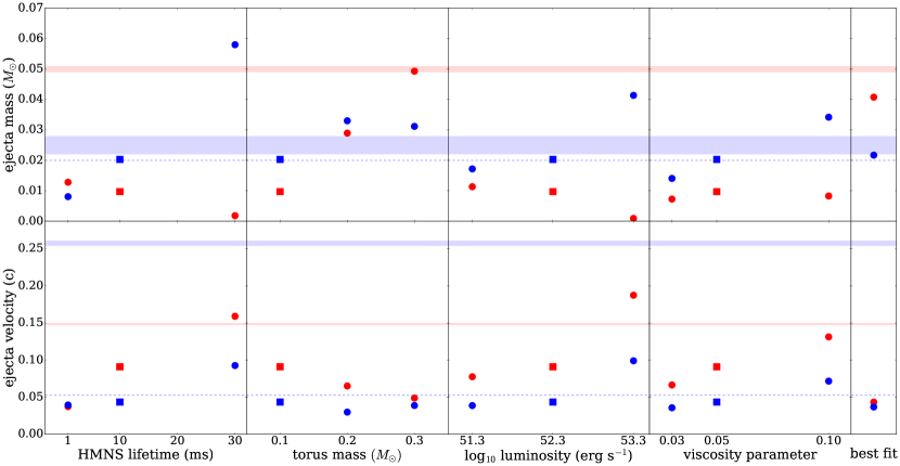
Figure 1: Ejected mass (top) and mass-averaged velocity (bottom) of the unbound disk outflow as a function of selected parameters: HMNS lifetime, initial torus mass, initial HMNS neutrino/antineutrino luminosity, and $\alpha$-viscosity parameter. The rightmost panel shows our ‘best fit’ model. Red and blue symbols denote lanthanide-rich ($Y_{e}<0.25$) and poor material, respectively, with squares denoting our ‘base’ model (Table 1). Data points have a fiducial uncertainty of $10\%$ due to resolution. The horizontal red and blue bands correspond to the two-component fit of GW170817 by Villar et al. (2017), while the horizontal dotted blue line corresponds to the (average) disk outflow values used by Kawaguchi et al. (2018).

3 Results

3.1 Overview of Disk Evolution

The qualitative evolution of the torus is independent of parameter choices, for details see MF14 and Lippuner et al. (2017). While the HMNS is present, accretion of the disk forms a high-density ($\sim 10^{12}\;\rm{g\;cm}^{-3}$) boundary layer around the HMNS. Due to intense neutrino and viscous heating, material is ejected from the boundary layer and from the edges of the disk on the local thermal time ($\sim 10$ ms). Material escaping within $\sim 20$ deg of the polar axis has $Y_{e}\sim 0.5$ due to strong irradiation, while on the equator the outflow has a $Y_{e}$ closer to the initial disk value. The bulk of the disk remains neutron-rich ($Y_{e}\sim 0.2$) due the higher densities and shadowing of neutrino irradiation.

Upon collapse of the HMNS into a BH, the boundary layer accretes within $\sim 0.1$ ms, and a rarefaction wave is launched outward. The torus readjusts on the equatorial plane, evacuating the polar funnel. After a viscous time ($\sim 100-300$ ms), weak interactions freeze out and mass is ejected due to heating by viscosity and nuclear recombination. By this time the electron fraction of the outflow is higher than the initial disk value due to the lower degeneracy ($Y_{e}\sim 0.2-0.3$).

3.2 Parameter Sensitivity

Table 1 shows the mass and mass-averaged radial velocity of unbound disk ejecta for all models, as measured at a radius $r=10^{9}$ cm. We use $Y_{e}=0.25$ to divide the ejecta into lanthanide-poor (‘blue’) and lanthanide-rich (‘red’) material (e.g., Lippuner & Roberts 2015). Figure 1 illustrates the most sensitive parameter dependencies. While here we use the two-component fit of Villar et al. (2017) as a reference observational result, our general conclusions are independent of the specific (multi-component) kilonova fit used.

Our baseline model ejects an amount of mass with $Y_{e}>0.25$ that approaches the observationally-inferred value, but there is insufficient lanthanide-rich mass ejected by a factor of $5$. Also, the average velocity of the blue component is lower than that of the red ejecta, with the latter being $0.09c$ only.

The larger amount of blue relative to red ejecta for the default HMNS lifetime ($\sim 10$ ms) differs from that obtained by MF14, because the latter used a non-spinning BH after HMNS collapse. The red ejecta is produced in the initial thermal expansion of the disk on the side of the torus opposite to the HMNS, before weak interactions have time to significantly reprocess the disk composition, and therefore depends entirely on the initial condition chosen in the baseline model ($Y_{e}=0.1$). Model ye25 imposes $Y_{e}=0.25$ initially in the disk, resulting in negligible red ejecta.

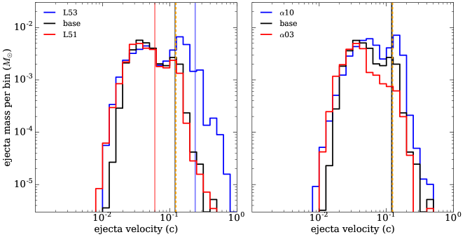
Figure 2: Mass histogram of unbound material ejected at $r=10^{9}$ cm, as a function of velocity, for models that vary the magnitude of the initial HMNS luminosity (left) and the viscosity parameter (right), as labeled. The vertical solid lines show the asymptotic velocity for a pure neutrino driven wind (equation 1), and the vertical dashed line shows the maximum velocity achievable from alpha particle recombination energy alone (equation 2).

Increasing the HMNS lifetime, viscosity parameter, or initial HMNS luminosity results in the same trend: higher blue mass ejected, constant or decreasing red mass, and moderate increase in the outflow velocities. In all cases, the average velocity of the blue ejecta does not exceed $0.1c$, and the red ejecta exceeds $0.15c$ only when its mass is $\ll 0.01M_{\odot}$. The physics behind this trend is different in each case: longer HMNS lifetime results in longer neutrino irradiation and absence of mass/energy loss to the BH, higher viscosity parameter increases viscous heating (thereby increasing the entropy and thus equilibrum $Y_{e}$) and accelerates the disk evolution, while a higher HMNS luminosity increases the strength of neutrino heating and accelerates the rate of change of $Y_{e}$.

Increasing the torus mass increases the lanthanide-rich mass, in part due to a larger thermal outflow that contains the most neutron-rich material, but also because the late-time viscous outflow becomes more neutron-rich. The blue mass peaks at $M_{t}=0.2M_{\odot}$ and then decreases for higher tori masses. The average velocities of both components remain below $0.05c$.

Changes in the initial torus properties other than mass or composition produce minor quantitative changes, as illustrated by models rt60 and s10. Similarly, changes in the mass of the central object yield the same qualitative result. Increasing the HMNS radius increases the surface area of the star and decreases the density in the boundary layer, resulting in stronger torus irradiation and thus a higher electron fraction in the outflow. However, the total ejected mass is not significantly affected. We caution that these effects may be unique to our treatment of the HMNS as a hard boundary.

Finally, our best fit model involves increasing the torus mass and formation radius. The combination of these effects creates outflows with red and blue masses close to observational fits (allowing for an additional $0.01M_{\odot}$ supplement of red dynamical ejecta), but with lower average velocities for the blue component than required.

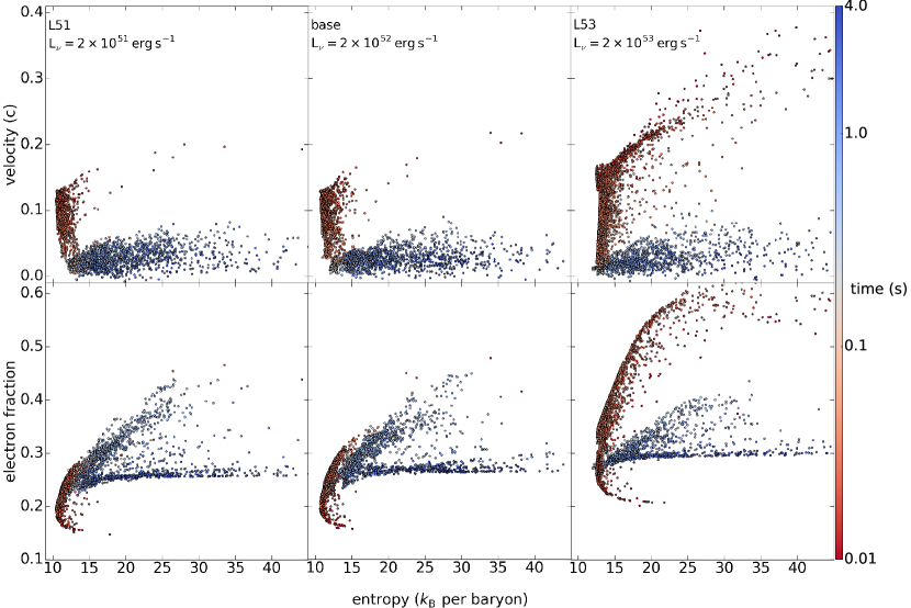
Figure 3: Properties of tracer particles ejected with positive energy, for models that vary the HMNS luminosity, as labeled, illustrating the different components of the disk outflow. The color of each particle corresponds to the time at which the temperature is $T=5\times 10^{9}$ K for the last time before ejection. The velocity, electron fraction, and entropy shown are the values attained at this time.

3.3 Physical constraints on the outflow velocity

The initial thermal outflow is launched by a combination of viscous and neutrino heating. Viscous angular momentum transport enhances the outflow relative to a pure neutrino driven wind, by transporting material to shallower regions of the potential well, in addition to enhancing energy deposition (Lippuner et al., 2017).

Figure 2 illustrates the magnitude of this effect for models that vary the neutrino luminosity and viscosity parameter. The velocity distribution of the outflow is broad, and always exceeds the asymptotic velocity obtained in steady-state neutrino-driven wind models (Thompson et al., 2001; Metzger et al., 2018)

$$v_{\nu}\approx 0.12c\bigg{(}\frac{L_{\nu}}{2\times 10^{52}}\bigg{)}^{0.3}.$$ (1)

The low-velocity portion of the distribution is ubiquitous to all models, arising from the late-time viscous/recombination-driven outflow which is launched once the disk has spread to larger radii. This component has an upper limit close to the maximum velocity that can be gained from nuclear recombination of alpha particles

$$v_{\rm rec}=\sqrt{2B_{\alpha}/m_{\alpha}}\approx 0.12c,$$ (2)

where $B_{\alpha}$ and $m_{\alpha}$ are nuclear binding energy and mass of an alpha particle (see, e.g., Fernández et al. 2018).

The different components of the outflow can be separated with tracer particles (Lippuner et al., 2017), as shown in Figure 3 for the models that vary the neutrino luminosity. The prompt ($t<0.1$ s) neutrino-driven wind appears as a tight correlation between the entropy and electron fraction of the particles. The importance of this component increases significantly with increasing neutrino luminosity, with the correlation extending to higher velocities and electron fractions. An intermediate component ($0.1<t<1$ s) also shows a correlation between entropy and electron fraction extending up to $Y_{e}=0.4$, but with a larger scatter than the prompt outflow and a lower velocity ($<0.1c$). The late-time viscous/recombination-powered wind in the advective phase ($t>1$ s) has nearly constant average velocity ($\lesssim 0.05c$) and electron fraction ($\lesssim 0.3$), but with a wide range of entropies.

Out of these components, only the prompt viscously-enhanced neutrino-driven wind is able to significantly exceed $0.1c$. However, in our most extreme case (model L53), the ejected mass with speeds above $0.2c$ and $Y_{e}>0.25$ is less than $3\times 10^{-3}M_{\odot}$.

We conclude that a combination of neutrino heating and viscous angular momentum transport in hydrodynamics is not able to account for the observed components of the GW170817 when considering the HMNS disk outflow alone. This conclusion is not altered by our omission of full general relativistic effects, since the dynamics close to the BH horizon is not a key element for the generation of outflows while the HMNS is present, and our results are consistent with those of Fujibayashi et al. (2018), who include all relativistic effects.

3.4 Homologous disk ejecta

For reference, we provide fits to our disk ejecta once it has reached homologous expansion, as needed for radiative transfer models. We compute the evolution into this phase ($\sim 1000$ s after merger) following the same method as in Kasen et al. (2015). Figure 4 shows the density and electron fraction profiles for the baseline model in this phase. For the ejecta density, we obtain acceptable fits with a broken power-law over a finite velocity range:

$$\rho/\rho_{0}=\Bigg{\{}\begin{array}[]{ll}(v/v_{0})^{-\eta_{0}}&v_{0}<v<v_{1}\\ (v_{1}/v_{0})^{-\eta_{0}}\,(v/v_{1})^{-\eta_{1}}&v_{1}<v<v_{2},\end{array}$$ (3)

where $\rho$ and $v$ are the ejecta density and radial velocity, respectively. The velocity range $[v_{0},v_{2}]$ is fixed by requiring that $90\%$ of the energy is kinetic, and it is beyond the turbulent region ($r>1.26\times 10^{6}$ km). The remaining variables $(\rho_{0},v_{1},\eta_{0},\eta_{1})$ are fit parameters.

The electron fraction has a more complicated behavior, hence we do not attempt to fit it. Parameters for equation (3) and average electron fraction are given in the right panel of Figure 4.

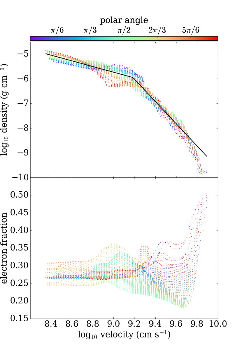
Model	$\rho_{0}/10^{-5}$	$v_{0}/c$	$v_{1}/c$	$v_{2}/c$	$\eta_{0}$	$\eta_{1}$	$\bar{Y}_{e}$
	(g cm-3)	($10^{-3}$)	($10^{-2}$)	($10^{-1}$)
base	1.024	7.479	5.101	2.604	1.150	4.503	0.264
a10	0.745	7.771	6.119	2.872	1.125	3.678	0.287
a03	4.485	6.955	3.827	2.371	1.788	4.858	0.260
t01	2.414	7.172	5.347	1.443	1.665	7.671	0.238
t30	0.585	7.739	5.337	3.146	0.875	2.946	0.354
M2.7	2.195	7.138	4.619	2.696	1.479	4.154	0.269
M2.6	2.430	7.109	6.632	2.459	1.741	5.276	0.257
L51	1.893	7.488	5.234	2.314	1.525	4.708	0.254
L53	1.667	7.535	4.728	4.349	1.512	3.252	0.354
mt03	6.673	6.828	4.586	2.263	1.404	5.266	0.233
mt02	3.714	6.822	3.461	2.501	0.996	4.376	0.242
rt60	3.551	6.868	5.747	2.251	1.818	5.589	0.242
rs30	2.543	7.214	4.126	2.019	1.445	5.197	0.233
s10	1.601	7.414	4.352	2.366	1.125	4.936	0.235
ye25	1.299	7.463	4.091	2.482	1.095	4.010	0.311
best	6.284	6.623	4.597	2.415	1.354	5.673	0.233

Figure 4: Left: Ejecta in the homologous phase for the base model ($t=1000$s), shown as density (top) and electron fraction (bottom) as a function of radial velocity in each computational cell, colored by polar angle. The solid line shows a broken power-law fit to the density profile. Right: Parameters of the broken power-law fit to the density in homology (equation 3). For reference, we also provide the mass-averaged electron fraction of the outflow.

4 Summary and Discussion

We have studied the long-term outflows from disks around HMNS remnants that collapse into BHs, using axisymmetric hydrodynamic simulations that include the dominant physical effects save for magnetic stresses. We find that for plausible parameters compatible with GW170817, hydrodynamic disk outflow models that employ shear viscosity to transport angular momentum cannot achieve mass-averaged velocities compatible with the blue kilonova as inferred from multi-component kilonova fits. While the ejected mass can in principle be brought closer to the inferred values by a suitable parameter choice, the same cannot be achieved for the velocities of both components.

Kawaguchi et al. (2018) find that radiative transfer simulations that include reprocessing of photons from the disk outflow by the dynamical ejecta do not require a disk wind expanding faster than $0.1c$ to explain the GW170817 kilonova. Here the dynamical ejecta provides a velocity boost to these blue photons, and eliminates the need for high ejecta masses, bringing it into agreement with current predictions from numerical relativity simulations. Our disk outflow models are fully compatible with their results (c.f. Figure 1). Establishing whether this is the correct resolution to the wind velocity problem requires further work.

Alternatively, state-of-the-art numerical relativity simulations predict too little dynamical ejecta to reconcile the large masses moving at $0.25c$. Enhancements in this prompt ejecta can be obtained for example by viscous effects, either by ejecting material directly from the HMNS at early times (Shibata et al., 2017b), or by thermally boosting the dynamical ejecta (Radice et al., 2018). The robustness of these effects remains to be further explored.

The only remaining way to significantly boost the disk velocities are magnetic stresses. Initial three-dimensional GRMHD models of BH remnant disks show that this can easily be achieved (Siegel & Metzger, 2018; Fernández et al., 2018). The conjecture is further supported by early-phase simulations of magnetized, differentially rotating HMNS remnants (e.g., Kiuchi et al. 2012; Siegel et al. 2014). Including the effects of magnetic fields is the most straightforward way to improve our simulations.

References

- Abbott et al. (2017a) Abbott, B. P., Abbott, R., Abbott, T. D., et al. 2017a, ApJ, 848, L13
- Abbott et al. (2017b) Abbott, B. P., et al. 2017b, ApJ, 848, L12
- Artemova et al. (1996) Artemova, I. V., Bjoernsson, G., & Novikov, I. D. 1996, ApJ, 461, 565
- Bauswein et al. (2017) Bauswein, A., Just, O., Janka, H.-T., & Stergioulas, N. 2017, ApJ, 850, L34
- Côté et al. (2018) Côté, B., Fryer, C. L., Belczynski, K., et al. 2018, ApJ, 855, 99
- Cowperthwaite et al. (2017) Cowperthwaite, P. S., et al. 2017, ApJ, 848, L17
- Dessart et al. (2009) Dessart, L., Ott, C. D., Burrows, A., Rosswog, S., & Livne, E. 2009, ApJ, 690, 1681
- Drout et al. (2017) Drout, M. R., et al. 2017, Science, 358, 1570
- Dubey et al. (2009) Dubey, A., Antypas, K., Ganapathy, M. K., et al. 2009, Parallel Computing, 35, 512
- Fernández & Metzger (2013) Fernández, R., & Metzger, B. D. 2013, MNRAS, 435, 502
- Fernández et al. (2018) Fernández, R., Tchekhovskoy, A., Quataert, E., Foucart, F., & Kasen, D. 2018, MNRAS, in press, arXiv:1808.00461
- Fontes et al. (2015) Fontes, C. J., Fryer, C. L., Hungerford, A. L., et al. 2015, High Energy Density Physics, 16, 53
- Fryxell et al. (2000) Fryxell, B., Olson, K., Ricker, P., et al. 2000, ApJS, 131, 273
- Fujibayashi et al. (2018) Fujibayashi, S., Kiuchi, K., Nishimura, N., Sekiguchi, Y., & Shibata, M. 2018, ApJ, 860, 64
- Hanauske et al. (2017) Hanauske, M., Takami, K., Bovard, L., et al. 2017, Phys. Rev. D, 96, 043004
- Hotokezaka et al. (2013) Hotokezaka, K., Kiuchi, K., Kyutoku, K., et al. 2013, Phys. Rev. D, 87, 024001
- Hunter (2007) Hunter, J. D. 2007, Computing In Science & Engineering, 9, 90
- Just et al. (2015) Just, O., Bauswein, A., Ardevol Pulpillo, R., Goriely, S., & Janka, H.-T. 2015, MNRAS, 448, 541
- Kasen et al. (2013) Kasen, D., Badnell, N. R., & Barnes, J. 2013, ApJ, 774, 25
- Kasen et al. (2015) Kasen, D., Fernández, R., & Metzger, B. D. 2015, MNRAS, 450, 1777
- Kasen et al. (2017) Kasen, D., Metzger, B., Barnes, J., Quataert, E., & Ramirez-Ruiz, E. 2017, Nature, 551, 80
- Kawaguchi et al. (2018) Kawaguchi, K., Shibata, M., & Tanaka, M. 2018, ApJ, 865, L21
- Kiuchi et al. (2012) Kiuchi, K., Kyutoku, K., & Shibata, M. 2012, PRD, 86, 064008
- Li & Paczyński (1998) Li, L.-X., & Paczyński, B. 1998, ApJ, 507, L59
- Lippuner et al. (2017) Lippuner, J., Fernández, R., Roberts, L. F., et al. 2017, MNRAS, 472, 904
- Lippuner & Roberts (2015) Lippuner, J., & Roberts, L. F. 2015, ApJ, 815, 82
- Margalit & Metzger (2017) Margalit, B., & Metzger, B. D. 2017, ApJ, 850, L19
- Metzger & Fernández (2014) Metzger, B. D., & Fernández, R. 2014, MNRAS, 441, 3444
- Metzger et al. (2018) Metzger, B. D., Thompson, T. A., & Quataert, E. 2018, ApJ, 856, 101
- Metzger et al. (2010) Metzger, B. D., Martínez-Pinedo, G., Darbha, S., et al. 2010, MNRAS, 406, 2650
- Perego et al. (2014) Perego, A., Rosswog, S., Cabezón, R. M., et al. 2014, MNRAS, 443, 3134
- Radice et al. (2018) Radice, D., Perego, A., Hotokezaka, K., et al. 2018, ApJL, in press, arXiv:1809.11163
- Richers et al. (2015) Richers, S., Kasen, D., O’Connor, E., Fernández, R., & Ott, C. D. 2015, ApJ, 813, 38
- Shakura & Sunyaev (1973) Shakura, N. I., & Sunyaev, R. A. 1973, A&A, 24, 337
- Shibata et al. (2017a) Shibata, M., Fujibayashi, S., Hotokezaka, K., et al. 2017a, Phys. Rev. D, 96, 123012
- Shibata & Kiuchi (2017) Shibata, M., & Kiuchi, K. 2017, Phys. Rev. D, 95, 123003
- Shibata et al. (2017b) Shibata, M., Kiuchi, K., & Sekiguchi, Y.-i. 2017b, PRD, 95, 083005
- Siegel et al. (2014) Siegel, D. M., Ciolfi, R., & Rezzolla, L. 2014, ApJ, 785, L6
- Siegel & Metzger (2018) Siegel, D. M., & Metzger, B. D. 2018, ApJ, 858, 52
- Tanaka (2016) Tanaka, M. 2016, Advances in Astronomy, 2016, 634197
- Tanaka & Hotokezaka (2013) Tanaka, M., & Hotokezaka, K. 2013, ApJ, 775, 113
- Tanaka et al. (2017) Tanaka, M., et al. 2017, PASJ, 69, 102
- Thompson et al. (2001) Thompson, T. A., Burrows, A., & Meyer, B. S. 2001, ApJ, 562, 887
- Timmes & Swesty (2000) Timmes, F. X., & Swesty, F. D. 2000, ApJS, 126, 501
- Villar et al. (2017) Villar, V. A., Guillochon, J., Berger, E., et al. 2017, ApJ, 851, L21