Trajectory PHD and CPHD filters

Abstract

This paper presents the probability hypothesis density filter (PHD) and the cardinality PHD (CPHD) filter for sets of trajectories, which are referred to as the trajectory PHD (TPHD) and trajectory CPHD (TCPHD) filters. Contrary to the PHD/CPHD filters, the TPHD/TCPHD filters are able to produce trajectory estimates from first principles. The TPHD filter is derived by recursively obtaining the best Poisson multitrajectory density approximation to the posterior density over the alive trajectories by minimising the Kullback-Leibler divergence. The TCPHD is derived in the same way but propagating an independent identically distributed (IID) cluster multitrajectory density approximation. We also propose the Gaussian mixture implementations of the TPHD and TCPHD recursions, the Gaussian mixture TPHD (GMTPHD) and the Gaussian mixture TCPHD (GMTCPHD), and the $L$-scan computationally efficient implementations, which only update the density of the trajectory states of the last $L$ time steps.

I Introduction

The probability hypothesis density (PHD) and cardinality PHD (CPHD) filters are widely used random finite set (RFS) algorithms for multitarget filtering, which aims to estimate the state of the targets at the current time based on a sequence of measurements [1, 2, 3, 4, 5, 6, 7]. These filters have been successfully used in different applications such as multitarget tracking [1], distributed multi-sensor fusion [8, 9], robotics [10, 11], computer vision [12, 13], road mapping [14] and sensor control [15].

The PHD/CPHD filters fit into the assumed density filtering framework and propagate a certain type of multitarget density on the current set of targets through the prediction and update steps [16]. The PHD filter considers a Poisson multitarget density, in which the cardinality of the set is Poisson distributed and, for each cardinality, its elements are independent and identically distributed (IID). On the other hand, the CPHD filter considers an IID cluster multitarget density, in which the cardinality distribution of the set is arbitrary and, for each cardinality, its elements are IID. If the output of either the prediction or the update step is no longer Poisson/IID cluster, the PHD/CPHD filters obtain the best Poisson/IID cluster approximation by minimising the Kullback-Leibler divergence (KLD).

The most important benefit of the PHD/CPHD filters is their low computational burden, as they avoid the measurement-to-target association problem. However, their main drawbacks are their relatively low performance in some scenarios [1, 17] and the fact that they do not build tracks, which denote sequences of target states that belong to the same target. The smoother versions of these filters [1, 18, 19] do not solve these drawbacks.

Despite the fact that the PHD/CPHD filters are unable to provide tracks in a mathematically rigorous way, several track building procedures have been proposed [20, 21, 22, 23, 24]. A track building procedure for PHD/CPHD filters was proposed in [25] by adding labels [26, 27] to the target states. Nonetheless, in the resulting labelled Poisson and labelled IID cluster densities, there is total confusion in the label-to-target association so they are not useful for track formation [25, Sec. III.B][28, Sec. II.B]. To solve this issue in [25], apart from the unique labels, unique tags are added to the PHD components, as in [22], and the original PHD/CPHD recursions are applied. However, in the considered posterior density, the tags are not part of the target state and are marginalised out. Therefore, the posterior is still distributed as labelled Poisson or labelled IID cluster and, theoretically, it does not have information to infer tracks. While tagging PHD components works well in some scenarios, each PHD component does not generally represent information about a unique target, as the corresponding number of targets is Poisson distributed. In fact, adding tags to the PHD components and reporting estimates with unique tags to build trajectories, can lead to track switches, missed detections and false targets when there is more than one target represented by the same tag.

In this paper, we address the intrinsic inability of standard PHD/CPHD filters to infer trajectories by developing PHD/CPHD filters that provide tracks from first principles, without adding labels or tags. We propose the trajectory PHD (TPHD) and trajectory CPHD (TCPHD) filters, which follow the same assumed density filtering scheme as the PHD/CPHD filters [29] with a fundamental difference: instead of using a set of targets as the state variable, they use a set of trajectories [30, 28].

The TPHD filter propagates a Poisson multitrajectory density on the space of sets of trajectories through the prediction and update steps, with a KLD minimisation after the update step. A diagram of the resulting Bayesian recursion is given in Figure 1. Similarly, the TCPHD filter propagates an IID cluster multitrajectory density and performs a KLD minimisation after the prediction and update steps, see Figure 2. Due to the widespread use of PHD/CPHD filters, this paper covers an important gap in the literature, as we show how PHD/CPHD filtering can be endowed with the ability to infer trajectories in a rigorous and principled way. In particular, the TPHD and TCPHD filters are able to estimate the trajectories of the alive targets by propagating a Poisson and an IID cluster multitrajectory density through the filtering recursion using KLD minimisations. The TPHD and TCPHD filters also avoid the above-mentioned drawbacks of trajectory estimation based on labelling/tagging the PHD. Apart from theoretically sound track formation, the proposed filters also have the advantage, compared to previous track building procedures used in PHD/CPHD filters, that they can update the information regarding past states of the trajectories.

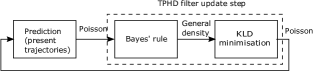
Figure 1: TPHD filter diagram for estimating the present trajectories at the current time. The TPHD filter assumes that the multitrajectory densities involved are Poisson (on the space of sets of trajectories). The output of Bayes’ rule is no longer Poisson but, in order to be able to perform the Bayesian recursion, it obtains the best Poisson approximation to the filtering density by minimising the KLD.

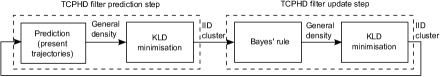
Figure 2: TCPHD filter diagram for estimating the present trajectories at the current time. The TCPHD filter assumes that the multitrajectory densities involved are IID cluster. The output of the prediction and Bayes’ rule are no longer IID clusters but the TCPHD filter obtains the best IID cluster approximation by minimising the KLD.

In this paper, we also propose Gaussian mixture implementations of the TPHD/TCPHD filters, which follow the spirit of the Gaussian mixture PHD/CPHD filters [3, 5]. The resulting Gaussian mixture TPHD (GMTPHD) and TCPHD (GMTCPHD) filters build trajectories under a Poisson or IID cluster approximation, whose PHD is represented by a Gaussian mixture. In this setting, a Gaussian component of the GMTPHD/GMTCPHD filter represents information over entire trajectories, while a Gaussian component in the Gaussian mixture PHD/CPHD filters (tagged or not) represents information over current target states. It is therefore straightforward to extract trajectory estimates from the GMTPHD/GMTCPHD filters. Additionally, we propose a version of the GMTPHD/GMTCPHD filters with lower computational burden called the $L$-scan GMTPHD/GMTCPHD filters. In practice, these filters only update the multitrajectory density of the trajectory states of the last $L$ time instant leaving the rest unaltered, which is quite efficient for implementation. The theoretical foundation of the $L$-scan GMTPHD filter is also based on the assumed density filtering framework and KLD minimisations. Preliminary results of this paper covering the TPHD filter were presented in [29].

The remainder of the paper is organised as follows. Section II presents background material on sets of trajectories. In Section III, we introduce the Poisson and IID cluster multitrajectory densities and some of their properties. The TPHD and TCPHD filters are derived in Sections IV and V, respectively. Their Gaussian mixture implementations are provided in Section VI. Simulation results are provided in Section VII. Finally, conclusions are drawn in Section VIII.

II Background

In this section, we describe some background material on multiple target tracking using sets of trajectories [28]. We review the considered variables, the set integral and cardinality distribution for sets of trajectories in Sections II-A, II-B and II-C, respectively. Finally, we introduce the PHD for sets of trajectories in Section II-D.

II-A Variables

A single target state $x\in\mathbb{R}^{n_{x}}$ contains information of interest about the target, e.g., its position and velocity. A set of single target states $\mathbf{x}$ belongs to $\mathcal{F}\left(\mathbb{R}^{n_{x}}\right)$ where $\mathcal{F}\left(\mathbb{R}^{n_{x}}\right)$ denotes the set of all finite subsets of $\mathbb{R}^{n_{x}}$. We are interested in estimating all target trajectories, where a trajectory consists of a sequence of target states that can start at any time step and end any time later on. Mathematically, a trajectory is represented as a variable $X=\left(t,x^{1:i}\right)$ where $t$ is the initial time step of the trajectory, $i$ is its length and $x^{1:i}=\left(x^{1},...,x^{i}\right)$ denotes a sequence of length $i$ that contains the target states at consecutive time steps of the trajectory.

We consider trajectories up to the current time step $k$. As a trajectory $\left(t,x^{1:i}\right)$ exists from time step $t$ to $t+i-1$, variable $\left(t,i\right)$ belongs to the set $I_{(k)}=\left\{\left(t,i\right):0\leq t\leq k\,\mathrm{and}\,1\leq i\leq k-t+1\right\}$. A single trajectory $X$ up to time step $k$ therefore belongs to the space $T_{\left(k\right)}=\uplus_{\left(t,i\right)\in I_{(k)}}\left\{t\right\}\times\mathbb{R}^{in_{x}}$, where $\uplus$ stands for disjoint union, which is used to highlight that the sets are disjoint. Similarly to the set ${\bf x}$ of targets, we denote a set of trajectories up to time step $k$ as $\mathbf{X}\in\mathcal{F}\left(T_{\left(k\right)}\right)$.

Given a trajectory $X=\left(t,x^{1:i}\right)$, the set $\tau^{k^{\prime}}\left(X\right)$, which can be empty, denotes the corresponding target state at a time step $k^{\prime}$. Given a set $\mathbf{X}$ of trajectories, the set $\tau^{k^{\prime}}\left(\mathbf{X}\right)$ of target states at time $k^{\prime}$ is $\tau^{k^{\prime}}\left(\mathbf{X}\right)=\bigcup_{X\in\mathbf{X}}\tau^{k^{\prime}}\left(X\right)$.

II-B Set integral

Given a real-valued function $\pi\left(\cdot\right)$ on the single trajectory space $T_{\left(k\right)}$, its integral is [28]

$$\int\pi\left(X\right)dX =\sum_{\left(t,i\right)\in I_{(k)}}\int\pi\left(t,x^{1:i}\right)dx^{1:i}.$$ (1)

This integral goes through all possible start times, lengths and target states of the trajectory. Given a real-valued function $\pi\left(\cdot\right)$ on the space $\mathcal{F}\left(T_{\left(k\right)}\right)$ of sets of trajectories, its set integral is [28]

$$\int\pi\left(\mathbf{X}\right)\delta\mathbf{X} =\sum_{n=0}^{\infty}\frac{1}{n!}\int\pi\left(\left\{X_{1},...,X_{n}\right\}\right)dX_{1:n}$$ (2)

where $X_{1:n}=\left(X_{1},...,X_{n}\right)$. A function $\pi\left(\cdot\right)$ is a multitrajectory density if $\pi\left(\cdot\right)\geq 0$ and its set integral is one.

II-C Cardinality distribution

Given a multitrajectory density $\pi\left(\cdot\right)$, its cardinality distribution is

$$\rho_{\pi}\left(n\right) =\frac{1}{n!}\int\pi\left(\left\{X_{1},...,X_{n}\right\}\right)dX_{1:n},$$ (3)

which is analogous to the case where there is a set of targets.

II-D Probability hypothesis density

The PHD [1] of a multitrajectory density $\pi\left(\cdot\right)$ is

$$D_{\pi}(X) =\int\pi\left(\left\{X\right\}\cup\mathbf{X}\right)\delta\mathbf{X}.$$ (4)

As in the PHD for RFS of targets, integrating the PHD in a region $A\subseteq T_{\left(k\right)}$ gives us the expected number of trajectories in this region [1, Eq. (4.76)]:

$$\hat{N}_{A} =\int_{A}D_{\pi}(X)dX$$

$$=\sum_{\left(t,i\right)\in I_{(k)}}\int 1_{A}\left(t,x^{1:i}\right)D_{\pi}(t,x^{1:i})dx^{1:i}$$ (5)

where $1_{A}\left(\cdot\right)$ is the indicator function of a subset $A$: $1_{A}\left(z\right)=1$ if $z\in A$ and $1_{A}\left(z\right)=0$ otherwise. Therefore, the expected number of trajectories up to time step $k$ is given by substituting $A=T_{\left(k\right)}$ into (5).

Example 1.

Let us consider a multitrajectory density $\nu\left(\cdot\right)$ with PHD

$$D_{\nu}\left(1,x^{1}\right) =\mathcal{N}\left(x^{1};10,1\right)+\mathcal{N}\left(x^{1};1000,1\right)$$ (6)

$$D_{\nu}\left(1,x^{1:2}\right) =\mathcal{N}\left(x^{1:2};\left(10,10.1\right),\left[\begin{array}[]{cc}1&1\\ 1&2\end{array}\right]\right),$$ (9)

and $D_{\nu}\left(X\right)=0$ for $X\neq\left(1,x^{1}\right)$ and $X\neq\left(1,x^{1:2}\right)$, where $\mathcal{N}\left(\cdot;m,P\right)$ is a Gaussian density with mean $m$ and covariance matrix $P$. The expected number of trajectories that start at time one with length 1 is given by substituting $A=\left\{1\right\}\times\mathbb{R}^{n_{x}}$ into (5) so

$$\hat{N}_{A} =\int D_{\nu}\left(1,x^{1}\right)dx^{1}=2.$$

The expected number of trajectories up to time step $k=2$ is $\hat{N}_{T_{\left(k\right)}}=3$. $\oblong$

III Poisson and IID cluster trajectory RFSs

In this section, we explain the Poisson and IID cluster trajectory RFSs.

III-A Multitrajectory densities

III-A1 Poisson RFS

For a Poisson RFS, the cardinality of the set is Poisson distributed and, for each cardinality, its elements are IID. A Poisson multitrajectory density $\nu\left(\cdot\right)$ has the form

$$\nu\left(\left\{X_{1},...,X_{n}\right\}\right) =e^{-\lambda_{\nu}}\lambda_{\nu}^{n}\prod_{j=1}^{n}\breve{\nu}\left(X_{j}\right)$$ (10)

where $\breve{\nu}\left(\cdot\right)$ is a single trajectory density, which implies

$$\int\breve{\nu}\left(X\right)dX =1,$$ (11)

and $\lambda_{\nu}\geq 0$. A Poisson multitrajectory density is characterised by either its PHD $D_{\nu}(X)=\lambda_{\nu}\breve{\nu}\left(X\right)$ or by $\lambda_{\nu}$ and $\breve{\nu}\left(\cdot\right)$ [1]. As a result, using (5), the expected number of trajectories is $\hat{N}_{T_{\left(k\right)}}=\lambda_{\nu}$. Further, its cardinality distribution is given by

$$\rho_{\nu}\left(n\right)=\frac{1}{n!}\int\nu\left(\left\{X_{1},...,X_{n}\right\}\right)dX_{1:n} =\frac{1}{n!}e^{-\lambda_{\nu}}\lambda_{\nu}^{n}.$$ (12)

Example 2.

We consider a Poisson RFS with the PHD of Example 1. Using (12), its cardinality distribution is Poisson with $\lambda_{\nu}=3$ and, therefore, its single trajectory density is $\breve{\nu}\left(X\right)=D_{\nu}\left(X\right)/3$. $\oblong$

III-A2 IID cluster RFS

For an IID cluster RFS with multitrajectory density $\nu\left(\cdot\right)$, the cardinality is distributed according to the probability mass function $\rho_{\nu}\left(\cdot\right)$ and, for each cardinality, its elements are IID according to a single trajectory density $\breve{\nu}\left(\cdot\right)$. The resulting multitrajectory density is

$$\nu\left(\left\{X_{1},...,X_{n}\right\}\right) =\rho_{\nu}\left(n\right)n!\prod_{j=1}^{n}\breve{\nu}\left(X_{j}\right).$$ (13)

As $\breve{\nu}\left(\cdot\right)$ is a single trajectory density, it meets (11). The PHD of (13) is given by [1]

$$D_{\nu}\left(x\right) =\breve{\nu}\left(x\right)\sum_{n=0}^{\infty}n\rho_{\nu}\left(n\right)$$ (14)

where the second factor corresponds to the expected number of trajectories. An IID cluster density can be characterised either by $\rho_{\nu}\left(\cdot\right)$ and $\breve{\nu}\left(\cdot\right)$, or by $\rho_{\nu}\left(\cdot\right)$ and $D_{\nu}\left(\cdot\right)$. How to draw samples from an IID cluster trajectory RFS, which includes the Poisson trajectory RFS as a particular case, is explained in Appendix A in the supplementary material.

III-B KLD minimisation

In this subsection, we provide two KLD minimisation theorems for Poisson and IID cluster multitrajectory densities, which will be used to derive the trajectory PHD/CPHD filters.

The KLD $\mathrm{D}\left(\pi\left\|\nu\right.\right)$ between multitrajectory densities $\pi\left(\cdot\right)$ and $\nu\left(\cdot\right)$ is given by [1]

$$\mathrm{D}\left(\pi\left\|\nu\right.\right) =\int\pi\left(\mathbf{X}\right)\log\frac{\pi\left(\mathbf{X}\right)}{\nu\left(\mathbf{X}\right)}\delta\mathbf{X}.$$ (15)

Then, the following theorems hold:

Theorem 3.

Given a multitrajectory density $\pi\left(\cdot\right)$, the Poisson multitrajectory density $\nu\left(\cdot\right)$ that minimises the KLD $\mathrm{D}\left(\pi\left\|\nu\right.\right)$ is characterised by the PHD $D_{\nu}\left(\cdot\right)=D_{\pi}\left(\cdot\right)$.

Theorem 4.

Given a multitrajectory density $\pi\left(\cdot\right)$, the IID cluster multitrajectory density $\nu\left(\cdot\right)$ that minimises the KLD $\mathrm{D}\left(\pi\left\|\nu\right.\right)$ is characterised by the PHD $D_{\nu}\left(\cdot\right)=D_{\pi}\left(\cdot\right)$ and the cardinality distribution $\rho_{\nu}\left(\cdot\right)=\rho_{\pi}\left(\cdot\right)$.

Theorem 3 is proved in Appendix A in [29]. The analogous theorem for sets of targets was proved in [31]. Theorem 4 is proved in Appendix B in the supplementary material. The analogous theorem for sets of targets was proved in [32, 16]. It should be noted that, as a Poisson RFS is a special type of IID cluster RFS, the best fitting IID cluster RFS always has a lower or equal KLD than the best fitting Poisson RFS.

III-C Inference only on alive trajectories

In this section, we explain why the TPHD and TCPHD filters are mainly useful to approximate the posterior multitrajectory density over alive trajectories, but not the posterior over all trajectories, which also include dead trajectories. This serves as a motivation to present the TPHD and TCPHD filters for tracking only the alive trajectories in the next sections.

Let us first explain why the TPHD filter, which considers a Poisson approximation, is only useful for the alive trajectories [29, Sec. V.B], though it was derived in [29] for dead and alive trajectories. In the prediction step, the part of the PHD that represents a trajectory that dies at the current time step is multiplied by the probability of death (one minus the probability of survival) [29, Thm. 5], which is usually low. As time goes on, the part of the PHD that represents dead trajectories never changes. As a result, even if a trajectory exists with a very high probability at some point in time, once it dies, the TPHD filter over all trajectories indicates that it existed with a very low probability. Therefore, the TPHD does not contain accurate information about dead trajectories, though it does contain useful information about alive trajectories.

In the following, we argue with an example why the TCPHD filter, which considers an IID cluster approximation, should only consider alive trajectories, as the TPHD filter.

Example 5.

Let us consider that the posterior $\pi^{k}\left(\cdot\right)$ over the set of trajectories at time $k$ has $m$ trajectories with probability 1 so $\rho_{\pi^{k}}\left(m\right)=1$. In addition, $\pi^{k}\left(\cdot\right)$ indicates that there are $m_{d}$ dead trajectories with independent (single trajectory) densities $\breve{d}_{1}\left(\cdot\right),...,\breve{d}_{m_{d}}\left(\cdot\right),$ and $m_{a}$ alive trajectories with independent densities $\breve{a}_{1}\left(\cdot\right),...,\breve{a}_{m_{a}}\left(\cdot\right)$, where $m_{d}+m_{a}=m$. Note that we can obtain this kind of true posterior, without TPHD/TCPHD approximations, if the probability of detection is one, there is no clutter, targets are born independently and they are far from each other at all time steps. In Appendix C (see supplementary material), we compute the best IID cluster density approximation $\nu^{k}\left(\cdot\right)$ to $\pi^{k}\left(\cdot\right)$ using Theorem 4 and show that the cardinality distribution of the alive targets in $\nu^{k}\left(\cdot\right)$ is

$$\rho_{a}\left(n\right) =\left(\begin{array}[]{c}m\\ n\end{array}\right)\left(\frac{m_{a}}{m}\right)^{n}\left(1-\frac{m_{a}}{m}\right)^{m-n},$$ (18)

where $n\in\left\{0,1,...,m\right\}$. As the filtering recursion continues, the total number $m$ of trajectories can only increase. On the contrary, $m_{a}$ does not necessarily increase so after a sufficiently long time $\frac{m_{a}}{m}$ may become very small. Then, using the Poisson limit theorem, the cardinality distribution of the alive targets can be approximated as Poisson with parameter $m_{a}$ [33]. Therefore, even in this simple example in which the cardinality of the alive targets is known, the best IID cluster approximation of the whole trajectory posterior approximates the cardinality of the alive targets as a Poisson distribution. $\oblong$

The conclusion of the previous example is that, in the long run, an IID cluster RFS is not necessarily better than a Poisson RFS, both considered over all trajectories, to approximate the cardinality distribution of the alive targets. In most applications, the cardinality of the alive trajectories is considerably more important than the cardinality of the total number of trajectories. In this paper, we therefore focus on an IID cluster approximation of the alive trajectories to develop the TCPHD filter. This implies that the TCPHD filter has an arbitrary cardinality distribution for the alive targets, as the CPHD filter.

IV Trajectory PHD filter

In this section, we derive the TPHD filter for tracking the alive targets. The TPHD propagates the multitrajectory density of a Poisson RFS through the filtering recursion. In the update step, the TPHD filter uses Bayes’ rule followed by a KLD minimisation to approximate the posterior as Poisson, see Figure 1. In Section IV-A, we present the Bayesian filtering recursion for sets of trajectories. The prediction and update steps of the TPHD filter are given in Sections IV-B and IV-C, respectively.

IV-A Bayesian filtering recursion

The posterior multitrajectory density $\pi^{k}\left(\cdot\right)$ at time $k$, which denotes the density of set of trajectories present at time $k$ given all measurements up to time $k$, is calculated via the prediction and update steps:

$$\omega^{k}\left(\mathbf{X}\right) =\int f\left(\mathbf{X}\left|\mathbf{Y}\right.\right)\pi^{k-1}\left(\mathbf{Y}\right)\delta\mathbf{Y}$$ (19)

$$\pi^{k}\left(\mathbf{X}\right) =\frac{\ell^{k}\left(\mathbf{z}^{k}|\tau^{k}\left(\mathbf{X}\right)\right)\omega^{k}\left(\mathbf{X}\right)}{\ell^{k}\left(\mathbf{z}^{k}\right)}$$ (20)

where $f\left(\cdot\left|\cdot\right.\right)$ is the transition density, $\omega^{k}\left(\cdot\right)$ is the predicted density at time $k$, $\mathbf{z}^{k}$ is the set of measurements at time $k$, $\ell^{k}\left(\cdot|\tau^{k}\left(\mathbf{X}\right)\right)$ is the density of the measurements given the current RFS of targets and

$$\ell^{k}\left(\mathbf{z}^{k}\right) =\int\ell^{k}\left(\mathbf{z}^{k}|\tau^{k}\left(\mathbf{X}\right)\right)\omega^{k}\left(\mathbf{X}\right)\delta\mathbf{X}$$

is the density of the measurements given the predicted density $\omega^{k}\left(\cdot\right)$. The predicted density at time $k$ is the density of the set of trajectories present at time step $k$ given the measurements up to time step $k-1$. As we only take into account the present trajectories, the only term that changes in (19)-(20) with respect to considering all trajectories is $f\left(\cdot\left|\cdot\right.\right)$, see [34, Sec. IV.A] for a detailed explanation. The description of these models will be given in Sections IV-B and IV-C.

IV-B Prediction

We make the following assumptions in the prediction step:

• P1 Given the current set ${\bf x}$ of targets, each target $x\in{\bf x}$ survives with probability $p_{S}\left(x\right)$ and moves to a new state with a transition density $g\left(\cdot\left|x\right.\right)$, or dies with probability $1-p_{S}\left(x\right)$.

• P2 The multitarget state at the next time step is the union of the surviving targets and new targets, which are born independently with a Poisson multitarget density $\beta_{\tau}\left(\cdot\right)$.

• P3 The multitrajectory density $\pi^{k-1}\left(\cdot\right)$ of the trajectories present at time $k-1$ represents a Poisson RFS.

Note that we use subindex $\tau$ in densities on RFS of targets, as in $\beta_{\tau}\left(\cdot\right)$. Let $\mathbb{N}_{k}=\left\{1,...,k\right\}$. Then, the relation between predicted PHD at time $k$ and the PHD of the posterior at time $k-1$ is given by the following theorem.

Theorem 6 (TPHD filter prediction).

Under Assumptions P1-P3, the predicted PHD $D_{\omega^{k}}\left(\cdot\right)$ of the trajectories present at time $k$ is

$$D_{\omega^{k}}\left(X\right) =D_{\xi^{k}}\left(X\right)+D_{\beta^{k}}\left(X\right)$$ (21)

where

$$D_{\beta^{k}}\left(t,x^{1:i}\right) =D_{\beta_{\tau}}\left(x^{1}\right)1_{\left\{k\right\}}\left(t\right)$$

$$D_{\xi^{k}}\left(t,x^{1:i}\right) =p_{S}\left(x^{i-1}\right)g\left(x^{i}\left|x^{i-1}\right.\right)$$

$$\quad\times D_{\pi_{k-1}}\left(t,x^{1:i-1}\right)1_{\mathbb{N}_{k-1}}\left(t\right)$$

if $t+i-1=k$ or zero otherwise.

This theorem is proved in [29] for a more general case in which dead trajectories are considered. As mentioned in Section III-C, in this paper, we only present the results for alive trajectories, as the results are mainly useful in this case. The predicted PHD is the sum of the PHD $D_{\beta^{k}}\left(\cdot\right)$ of the trajectories born at time step $k$ and the PHD $D_{\xi^{k}}\left(\cdot\right)$ of the surviving trajectories. The end time of trajectory $\left(t,x^{1:i}\right)$ is $t+i-1$ so $D_{\omega^{k}}\left(t,x^{1:i}\right)$ is zero if $t+i-1\neq k$. For the surviving trajectories, we multiply the PHD by the transition density and the survival probability. Note that the provided PHD characterises the Poisson RFS that represents the predicted density.

IV-C Update

We make the following assumptions in the update step:

• U1 For a given multi-target state $\mathbf{x}$ at time $k$, each target state $x\in\mathbf{x}$ is either detected with probability $p_{D}\left(x\right)$ and generates one measurement with density $l\left(\cdot|x\right)$, or missed with probability $1-p_{D}\left(x\right)$.

• U2 The measurement $\mathbf{z}^{k}$ is the union of the target-generated measurements and Poisson clutter with density $c\left(\cdot\right)$.

• U3 The multitrajectory density $\omega{}^{k}\left(\cdot\right)$ represents a Poisson RFS.

Let $\Xi_{n,n_{z}}$ denote the set that contains all the vectors $\sigma=\left(\sigma_{1},...,\sigma_{n}\right)$ that indicate associations of $n_{z}$ measurements to $n$ targets, which can be either detected or undetected. If $\sigma\in\Xi_{n,n_{z}}$, $\sigma_{i}=j\in\left\{1,...,n_{z}\right\}$ indicates that measurement $j$ is associated with target $i$ and $\sigma_{i}=0$ indicates that target $i$ has not been detected. Under Assumptions U1 and U2, which define the standard measurement model, the density of the measurement given the state is [1, Eq. (7.21)]

$$\ell^{k}\left(\left\{z_{1},...,z_{n_{z}}\right\}\left|\left\{x_{1},...,x_{n}\right\}\right.\right)$$

$$\quad=e^{-\lambda_{c}}\left[\prod_{i=1}^{n_{z}}\lambda_{c}\breve{c}\left(z_{i}\right)\right]\left[\prod_{i=1}^{n}\left(1-p_{D}\left(x_{i}\right)\right)\right]$$

$$\qquad\times\sum_{\sigma\in\Xi_{n,n_{z}}}\prod_{i:\sigma_{i}>0}\frac{p_{D}\left(x_{i}\right)l\left(z_{\sigma_{i}}|x_{i}\right)}{\left(1-p_{D}\left(x_{i}\right)\right)\lambda_{c}\breve{c}\left(z_{\sigma_{i}}\right)}.$$ (22)

where $\lambda_{c}$ and $\breve{c}\left(\cdot\right)$ characterise $c\left(\cdot\right)$, see (10).

Let $L_{\mathbf{z}^{k}}\left(\cdot\right)$ denote the PHD filter pseudolikelihood function, which is given by [1, Sec. 8.4.3]

$$L_{\mathbf{z}^{k}}\left(x\right) =1-p_{D}\left(x\right)+p_{D}\left(x\right)$$

$$\quad\times\sum_{z\in\mathbf{z}^{k}}\frac{l\left(z|x\right)}{\lambda_{c}\breve{c}\left(z\right)+\int p_{D}\left(y\right)l\left(z|y\right)D_{\omega_{\tau}^{k}}\left(y\right)dy}$$

with $D_{\omega_{\tau}^{k}}\left(\cdot\right)$ representing the PHD of the targets at time $k$ of density $\omega^{k}\left(\cdot\right)$, which is given by [29]

$$D_{\omega_{\tau}^{k}}\left(y\right) =\sum_{t=1}^{k}\int D_{\omega^{k}}\left(t,x^{1:k-t},y\right)dx^{1:k-t}.$$ (23)

Then, the TPHD filter update step is given by the following theorem:

Theorem 7 (TPHD filter update).

Under Assumptions U1-U3, the updated PHD $D_{\pi^{k}}\left(\cdot\right)$ at time $k$ is

$$D_{\pi^{k}}\left(t,x^{1:i}\right) =D_{\omega^{k}}\left(t,x^{1:i}\right)L_{\mathbf{z}^{k}}\left(x^{i}\right)$$

if $t+i-1=k$ or zero, otherwise.

This theorem is proved in [29] for a more general case in which dead trajectories are included. It should be noted that Bayes’ update (20) uses a likelihood (22) that involves a summation over all target-to-measurement associations in the multitarget space. In contrast, the TPHD filter update is similar to the PHD filter update in the sense that it uses a pseudolikelihood function $L_{\mathbf{z}^{k}}\left(\cdot\right)$ which is defined on the single target space and only involves associations between a single target and the measurements.

V Trajectory CPHD filter

In this section we present the trajectory CPHD (TCPHD) filter for tracking the alive targets. The TCPHD propagates the multitrajectory density of an IID cluster RFS through the filtering recursion. In the prediction and update steps, the TCPHD filter makes use of a KLD minimisation to obtain an IID cluster approximation, see Figure 2.

Prior to deriving the TCPHD filter, we provide some notation. Given two sequences $a\left(n\right)$ and $b\left(n\right)$, $n\in\mathbb{N}\cup\left\{0\right\}$, we denote

$$\left\langle a,b\right\rangle =\sum_{n=0}^{\infty}a\left(n\right)b\left(n\right).$$

Given a set $\mathbf{z}$, the elementary symmetric function of order $j$ is [5]

$$e_{j}\left(\mathbf{z}\right) =\sum_{\mathbf{s}\subseteq\mathbf{z},\left|S\right|=j}\left(\prod_{\zeta\in\mathbf{s}}\zeta\right)$$ (24)

with $e_{0}\left(Z\right)=1$ by convention. We also use $\setminus$ to denote set subtraction.

V-A Prediction

The TCPHD filter prediction is obtained under Assumptions P1 and the additional assumptions

• P4 The multitarget state at the next time step is the union of the surviving targets and new targets, which are born independently with an IID cluster multitarget density $\beta_{\tau}\left(\cdot\right)$.

• P5 The multitrajectory density $\pi^{k-1}\left(\cdot\right)$ represents an IID cluster RFS.

Under Assumption P4, the set of new born trajectories at time $k$ has cardinality $\rho_{\beta^{k}}\left(\cdot\right)=\rho_{\beta_{\tau}}\left(\cdot\right)$ and PHD

$$D_{\beta^{k}}\left(t,x^{1:i}\right) =\begin{cases}D_{\beta_{\tau}}\left(x^{1}\right)&t=k,\,i=1\\ 0&\mathrm{otherwise}.\end{cases}$$

The TCPHD filter prediction consists of applying the usual prediction step plus a KLD minimisation, which is performed by calculating the cardinality distribution and PHD of the predicted density, see Figure 2. The result is given in the following theorem.

Theorem 8 (TCPHD filter prediction).

Under Assumptions P1, P4 and P5, the PHD of the predicted density is the same as in the PHD filter, see Theorem 6. The cardinality distribution of the predicted density is

$$\rho_{\omega^{k}}\left(m\right) =\sum_{j=0}^{m}\rho_{\beta^{k}}\left(m-j\right)\sum_{n=j}^{\infty}\left(\begin{array}[]{c}n\\ j\end{array}\right)\rho_{\pi^{k-1}}\left(n\right)$$ (27)

$$\quad\times\frac{\left[\int\left(1-p_{S}(x)\right)D_{\pi_{\tau}^{k-1}}(x)dx\right]^{n-j}}{\left[\int D_{\pi_{\tau}^{k-1}}(x)dx\right]^{n}}$$

$$\quad\times\left[\int p_{S}\left(x\right)D_{\pi_{\tau}^{k-1}}(x)dx\right]^{j}$$ (28)

where $D_{\pi_{\tau}^{k-1}}\left(\cdot\right)$ is the PHD of the targets at time $k-1$ according to $\pi^{k-1}\left(\cdot\right)$, which is calculated as in (23).

Theorem 8 is proved in Appendix E (see supplementary material). The TCPHD filter prediction updates the cardinality distribution as the CPHD filter. The TCPHD does not integrate out past states of the trajectories in the PHD to keep trajectory information, while the CPHD filter does.

V-B Update

The TCPHD filter update is derived under Assumption U1 and the additional assumptions

• U4 The measurement $\mathbf{z}^{k}$ is the union of the target-generated measurements and IID cluster clutter with density $c\left(\cdot\right)$.

• U5 The multitrajectory density $\omega{}^{k}\left(\cdot\right)$ represents an IID cluster RFS.

As indicated in Figure 2, the TCPHD update consists of applying Bayes’ rule, see (20), followed by a KLD minimisation, which is performed as indicated by Theorem 4. We first consider the distribution of the present targets at the current time. Under Assumption U5, it is direct to obtain that the distribution of the targets present at time $k$ is also an IID cluster with cardinality distribution $\rho_{\omega^{k}}\left(\cdot\right)$ and PHD (23). The resulting TCPHD filter update is given in the following theorem.

Theorem 9 (TCPHD filter update).

Under Assumptions U1, U4 and U5, the cardinality distribution and the PHD of the posterior at time $k$ are

$$\rho_{\pi^{k}}\left(n\right) =\frac{\Upsilon^{0}\left[D_{\omega_{\tau}^{k}},\mathbf{z}^{k}\right]\left(n\right)\rho_{\omega^{k}}\left(n\right)}{\left\langle\Upsilon^{0}\left[D_{\omega_{\tau}^{k}},\mathbf{z}^{k}\right],\rho_{\omega^{k}}\right\rangle}$$ (29)

$$D_{\pi^{k}}\left(t,x^{1:i}\right) =\frac{\left\langle\Upsilon^{1}\left[D_{\omega_{\tau}^{k}},\mathbf{z}^{k}\right],\rho_{\omega^{k}}\right\rangle}{\left\langle\Upsilon^{0}\left[D_{\omega_{\tau}^{k}},\mathbf{z}^{k}\right],\rho_{\omega^{k}}\right\rangle}$$

$$\quad\times\left(1-p_{D}\left(x^{i}\right)\right)D_{\omega^{k}}\left(t,x^{1:i}\right)$$

$$\quad+\sum_{z\in\mathbf{z}^{k}}\frac{\left\langle\Upsilon^{1}\left[D_{\omega_{\tau}^{k}},\mathbf{z}^{k}\setminus\left\{z\right\}\right],\rho_{\omega^{k}}\right\rangle}{\left\langle\Upsilon^{0}\left[D_{\omega_{\tau}^{k}},\mathbf{z}^{k}\right],\rho_{\omega^{k}}\right\rangle}$$

$$\quad\times\frac{l\left(z|x^{i}\right)}{\breve{c}\left(z\right)}p_{D}\left(x^{i}\right)D_{\omega^{k}}(t,x^{1:i})$$ (30)

if $t+i-1=k$ or $D_{\pi^{k}}\left(t,x^{1:i}\right)=0$, otherwise, and

$$\Upsilon^{u}\left[D_{\omega_{\tau}^{k}},\mathbf{z}^{k}\right]\left(n\right) =\sum_{j=0}^{\min\left(\left|\mathbf{z}^{k}\right|,n-u\right)}\left(\left|\mathbf{z}^{k}\right|-j\right)!\rho_{c}\left(\left|\mathbf{z}^{k}\right|-j\right)$$

$$\quad\times\frac{\left[\int\left(1-p_{D}(x)\right)D_{\omega_{\tau}^{k}}(x)dx\right]^{n-\left(j+u\right)}}{\left[\int D_{\omega_{\tau}^{k}}(x)dx\right]^{n}}$$

$$\quad\times\frac{n!}{\left(n-j-u\right)!}e_{j}\left(\Xi\left(D_{\omega_{\tau}^{k}},\mathbf{z}^{k}\right)\right)$$ (31)

$$\Xi\left(D_{\omega_{\tau}^{k}},\mathbf{z}^{k}\right) =\left\{\int\frac{l\left(z|x\right)}{\breve{c}\left(z\right)}p_{D}\left(x\right)D_{\omega_{\tau}^{k}}(x)dx:z\in\mathbf{z}^{k}\right\}.$$

Theorem 9 is proved in Appendix D (see supplementary material). The update step of the TCPHD filter is equivalent to the CPHD filter, with the main difference that the updated PHD contains information about previous states of the trajectories.

VI Gaussian mixture implementations

In this section, we present the Gaussian mixture implementations of the TPHD and TCPHD filters. We use the notation

$$\mathcal{N}\left(t,x^{1:i};t^{k},m^{k},P^{k}\right) =\begin{cases}\mathcal{N}\left(x^{1:i};m^{k},P^{k}\right)&t=t^{k},\,i=i^{k}\\ 0&\mathrm{otherwise}\end{cases}$$ (32)

where $i^{k}=\mathrm{dim}\left(m^{k}\right)/n_{x}$. Equation (32) represents a single trajectory Gaussian density with start time $t^{k}$, duration $i^{k}$, mean $m^{k}\in\mathbb{R}^{i^{k}n_{x}}$ and covariance matrix $P^{k}\in\mathbb{R}^{i^{k}n_{x}\times i^{k}n_{x}}$ evaluated at $\left(t,x^{1:i}\right)$. We use $\otimes$ to indicate the Kronecker product and $0_{m,n}$ is the $m\times n$ zero matrix.

We make the additional assumptions

• A1 The probabilities $p_{S}$ and $p_{D}$ are constants.

• A2 $g\left(x^{i}\left|x^{i-1}\right.\right)=\mathcal{N}\left(x^{i};Fx^{i-1},Q\right)$.

• A3 $l\left(z|x\right)=\mathcal{N}\left(z;Hx,R\right)$.

• A4 The PHD of the birth density $\beta^{k}\left(\cdot\right)$ is

  $$D_{\beta^{k}}\left(X\right) =\sum_{j=1}^{J_{\beta}^{k}}w_{\beta,j}^{k}\mathcal{N}\left(X;k,m_{\beta,j}^{k},P_{\beta,j}^{k}\right)$$ (33)

  where $J_{\beta}^{k}\in\mathbb{N}$ is the number of components, $w_{\beta,j}^{k}$ is the weight of the $j$th component, $m_{\beta,j}^{k}\in\mathbb{R}^{n_{x}}$ its mean and $P_{\beta,j}^{k}\in\mathbb{R}^{n_{x}\times n_{x}}$ its covariance matrix.

It should be noted that $F\in\mathbb{R}^{n_{x}\times n_{x}}$ is the single-target transition matrix, $Q\in\mathbb{R}^{n_{x}\times n_{x}}$ is the covariance matrix of the single-target process noise, $H\in\mathbb{R}^{n_{z}\times n_{x}}$ is the single-measurement matrix and $R\in\mathbb{R}^{n_{z}\times n_{z}}$ is the covariance matrix of the single-measurement noise. In addition, the models provided by A1-A4 could be time varying but time is omitted for notational convenience. In the rest of this section, we present the Gaussian mixture implementations of the TPHD and TCPHD filters in Sections VI-A and VI-B, respectively. The $L$-scan versions of the filters and trajectory estimation are addressed in Sections VI-C and VI-D. Finally, a discussion is provided in Section VI-E.

VI-A Gaussian mixture TPHD filter

Under Assumptions A1-A4, P1-P3 and U1-U3, we can calculate the TPHD filter in closed form giving rise to the GMTPHD filter, whose prediction and update steps are provided in the following propositions.

Proposition 10 (GMTPHD filter prediction).

Assume $\pi^{k-1}\left(\cdot\right)$ has a PHD

$$D_{\pi^{k-1}}\left(X\right) =\sum_{j=1}^{J^{k-1}}w_{j}^{k-1}\mathcal{N}\left(X;t_{j}^{k-1},m_{j}^{k-1},P_{j}^{k-1}\right)$$

where $t_{j}^{k-1}+i_{j}^{k-1}-1=k-1$ with $i_{j}^{k-1}=\mathrm{dim}\left(m_{j}^{k-1}\right)/n_{x}$. Then, the PHD of $\omega^{k}\left(\cdot\right)$ is

$$D_{\omega^{k}}\left(X\right) =D_{\beta^{k}}\left(X\right)+p_{S}\sum_{j=1}^{J^{k-1}}w_{j}^{k-1}\mathcal{N}\left(X;t_{j}^{k-1},m_{\omega,j}^{k},P_{\omega,j}^{k}\right)$$ (34)

where

$$m_{\omega,j}^{k} =\left[\left(m_{j}^{k-1}\right)^{T},\left(\dot{F}_{j}m_{j}^{k-1}\right)^{T}\right]^{T},$$

$$\dot{F}_{j} =\left[0_{1,i_{j}^{k-1}-1},1\right]\otimes F,$$

$$P_{\omega,j}^{k} =\left[\begin{array}[]{cc}P_{j}^{k-1}&P_{j}^{k-1}\dot{F}_{j}^{T}\\ \dot{F}_{j}P_{j}^{k-1}&\dot{F}_{j}P_{j}^{k-1}\dot{F}_{j}^{T}+Q\end{array}\right].$$

Proposition 10 is a consequence of Theorem 6 and conventional properties of Gaussian densities. Compared to the GMPHD filter prediction, the main difference is that previous states are not integrated out.

Proposition 11 (GMTPHD filter update).

Assume $\omega^{k}\left(\cdot\right)$ has a PHD

$$D_{\omega^{k}}\left(X\right) =\sum_{j=1}^{J_{\omega}^{k}}w_{\omega,j}^{k}\mathcal{N}\left(X;t_{\omega,j}^{k},m_{\omega,j}^{k},P_{\omega,j}^{k}\right).$$ (35)

Then, the PHD of $\pi^{k}\left(\cdot\right)$ is

$$D_{\pi^{k}}\left(X\right) =\left(1-p_{D}\right)D_{\omega^{k}}\left(X\right)$$

$$\,+\sum_{z\in\mathbf{z}^{k}}\sum_{j=1}^{J^{k}}w_{j}\left(z\right)\mathcal{N}\left(X;t_{\omega,j}^{k},m_{j}^{k}\left(z\right),P_{j}^{k}\right)$$ (36)

where

$$w_{j}\left(z\right) =\frac{p_{D}w_{\omega,j}^{k}q_{j}\left(z\right)}{\lambda_{c}\breve{c}\left(z\right)+p_{D}\sum_{l=1}^{J_{\omega}^{k}}w_{\omega,l}^{k}q_{l}\left(z\right)}$$

$$\overline{z}_{j} =\dot{H}_{j}m_{\omega,j}^{k},\quad S_{j}=\dot{H}_{j}P_{\omega,j}^{k}\dot{H}_{j}^{T}+R$$

$$\dot{H}_{j} =\left[0_{1,i_{\omega,j}^{k}-1},1\right]\otimes H$$

$$q_{j}\left(z\right) =\mathcal{N}\left(z;\overline{z}_{j},S_{j}\right)$$

$$m_{j}^{k}\left(z\right) =m_{\omega,j}^{k}+P_{\omega,j}^{k}\dot{H}^{T}S_{j}^{-1}\left(z-\overline{z}_{j}\right)$$

$$P_{j}^{k} =P_{\omega,j}^{k}-P_{\omega,j}^{k}\dot{H}^{T}S_{j}^{-1}\dot{H}P_{\omega,j}^{k}.$$

and $i_{\omega,j}^{k}=\mathrm{dim}\left(m_{\omega,j}^{k}\right)/n_{x}$

Proposition 11 is a consequence of Theorem 7 and the Kalman filter update equations [35]. Also, the GMTPHD filter update is similar to the GMPHD filter update. The main differences is that the GMTPHD updates the whole trajectories.

VI-B Gaussian mixture TCPHD filter

The GMTCPHD filtering recursion requires Assumptions A1-A4, P1, P4, P5, U1, U4 and U5, and is given by the following propositions.

Proposition 12 (GMTCPHD filter prediction).

Assume the posterior $\pi^{k-1}\left(\cdot\right)$ has a cardinality distribution $\rho_{\pi^{k-1}}\left(\cdot\right)$ and a PHD

$$D_{\pi^{k-1}}\left(X\right) =\sum_{j=1}^{J^{k-1}}w_{j}^{k-1}\mathcal{N}\left(X;t_{j}^{k-1},m_{j}^{k-1},P_{j}^{k-1}\right).$$ (37)

Then, the TCPHD filter prediction yields

$$\rho_{\omega^{k}}\left(m\right) =\sum_{j=0}^{m}\rho_{\beta^{k}}\left(m-j\right)$$

$$\quad\times\sum_{n=j}^{\infty}\left(\begin{array}[]{c}n\\ j\end{array}\right)\rho_{\pi^{k-1}}\left(n\right)\left(1-p_{S}\right)^{n-j}p_{S}^{j}$$

$$D_{\omega^{k}}\left(X\right) =D_{\beta^{k}}\left(X\right)+p_{S}\sum_{j=1}^{J^{k-1}}w_{j}^{k-1}\mathcal{N}\left(X;t_{j}^{k-1},m_{\omega,j}^{k},P_{\omega,j}^{k}\right)$$

where $m_{\omega,j}^{k}$ and $P_{\omega,j}^{k}$ are given in Proposition 10.

Proposition 12 is a consequence of Theorem 8. The main difference with the GMCPHD filter is that the GMTCPHD filter does not integrate out previous states in the PHD. It should also be noted that the GMTPHD and the GMTCPHD propagate the PHD in the same way. The difference is that the GMTCPHD also considers the cardinality of $\omega^{k}\left(\cdot\right)$.

Proposition 13 (GMTCPHD filter update).

Assume the prior $\omega^{k}\left(\cdot\right)$ has a cardinality distribution $\rho_{\omega^{k}}\left(\cdot\right)$ and a PHD

$$D_{\omega^{k}}\left(X\right) =\sum_{j=1}^{J_{\omega}^{k}}w_{\omega,j}^{k}\mathcal{N}\left(X;t_{\omega,j}^{k},m_{\omega,j}^{k},P_{\omega,j}^{k}\right).$$ (38)

Then, the TCPHD filter update yields

$$\rho_{\pi^{k}}\left(n\right) =\frac{\Psi^{0}\left[w_{\omega}^{k},\mathbf{z}^{k}\right]\left(n\right)\rho_{\omega^{k}}\left(n\right)}{\left\langle\Psi^{0}\left[w_{\omega}^{k},\mathbf{z}^{k}\right],\rho_{\omega^{k}}\right\rangle}$$

$$D_{\pi^{k}}\left(X\right) =\frac{\left\langle\Psi^{1}\left[w_{\omega}^{k},\mathbf{z}^{k}\right],\rho_{\omega^{k}}\right\rangle}{\left\langle\Psi^{0}\left[w_{\omega}^{k},\mathbf{z}^{k}\right],\rho_{\omega^{k}}\right\rangle}\left(1-p_{D}\right)D_{\omega^{k}}\left(X\right)$$

$$\quad+\sum_{z\in\mathbf{z}^{k}}\sum_{j=1}^{J_{\omega}^{k}}w_{j}\left(z\right)\mathcal{N}\left(X;t_{\omega,j}^{k},m_{j}^{k}\left(z\right),P_{j}^{k}\right)$$

where

$$\Psi^{u}\left[w_{\omega}^{k},\mathbf{z}^{k}\right]\left(n\right) =\sum_{j=0}^{\min\left(\left|\mathbf{z}^{k}\right|,n-u\right)}\left(\left|\mathbf{z}^{k}\right|-j\right)!\rho_{c}\left(\left|\mathbf{z}^{k}\right|-j\right)$$

$$\quad\times\frac{\left(1-p_{D}\right)^{n-\left(j+u\right)}}{\left\langle 1,w_{\omega}^{k}\right\rangle^{j+u}}\frac{n!}{\left(n-j-u\right)!}$$

$$\quad\times e_{j}\left(\Lambda\left(w_{\omega}^{k},\mathbf{z}^{k}\right)\right)$$

$$\Lambda\left(w_{\omega}^{k},\mathbf{z}^{k}\right) =\left\{\frac{p_{D}}{\breve{c}\left(z\right)}\left(w_{\omega}^{k}\right)^{T}q\left(z\right):z\in\mathbf{z}^{k}\right\}$$

$$w_{\omega}^{k} =\left[w_{\omega,1}^{k},...,w_{\omega,J_{\omega}^{k}}^{k}\right]^{T}$$

$$q\left(z\right) =\left[q_{1}\left(z\right),...,q_{J_{\omega}^{k}}\left(z\right)\right]^{T}$$

$$w_{j}\left(z\right) =\frac{p_{D}w_{\omega,j}^{k}q_{j}\left(z\right)\left\langle\Psi^{1}\left[w_{\omega}^{k},\mathbf{z}^{k}\setminus\left\{z\right\}\right],\rho_{\omega^{k}}\right\rangle}{\breve{c}\left(z\right)\left\langle\Psi^{0}\left[w_{\omega}^{k},\mathbf{z}^{k}\right],\rho_{\omega^{k}}\right\rangle}$$

and $q_{j}\left(z\right)$, $m_{j}^{k}\left(z\right)$ and $P_{j}^{k}$ are given in Proposition 11.

Proposition 13 is a consequence of Theorem 9 and the Kalman filter update [35]. The GMTCPHD filter update is analogous to the GMCPHD filter [5], with the difference that previous states of the target trajectories are also included.

VI-C $L$-scan implementations

In this section, we propose the use of pruning and absorption to limit the number of components in the Gaussian mixture and a computationally efficient implementation of the Gaussian mixture filters: the $L$-scan GMTPHD and GMTCPHD filters.

The PHD of the GMTPHD/GMTCPHD filters has an increasing number of components as time progresses and, to limit complexity, we need to bound the number of components. We use the following techniques: pruning with threshold $\Gamma_{p}$, setting a maximum number $J_{max}$ of components and absorption [29]. Absorption consists of removing components of the PHD whose distribution of the current target state is close to the distribution of the current target state of another component with a higher weight, and adding the weights of the removed components to the weight of the component that has not been removed. Absorption is motivated by the fact that if two components have a very similar distribution over the current target state, based on a Mahalanobis distance criterion, future measurements will affect both component weights and future states in a similar way. Therefore, without absorption, we would have two components with practically the same Gaussian densities for the trajectory states corresponding to recent time steps, for which we would be repeating the same calculations. It should also be noted that single trajectory densities can be quite different in the past even if they are similar for the current target state. Therefore, a direct use of merging [36] for single trajectory densities, which would use moment matching at all time steps, can provide poor results and absorption is preferred. The steps of the pruning and absorption algorithms for the GMTPHD/GMTCPHD filters are given in Algorithm 1, where we use the notation $\Phi_{j}^{k}=\left(w_{j}^{k},t_{j}^{k},m_{j}^{k},P_{j}^{k}\right)$ .

Algorithm 1 Pruning and absorption for the GMTPHD and GMTCPHD filters

Input: Posterior PHD parameters $\left\{\Phi_{j}^{k}\right\}_{j=1}^{J^{k}}$, pruning threshold $\Gamma_{p}$, absorption threshold $\Gamma_{a}$, maximum number of terms $J_{max}$.

Output: Pruned posterior PHD parameters $\left\{\Phi_{o,j}^{k}\right\}_{j=1}^{\hat{J}^{k}}$

- Set $l=0$ and $I=\left\{j\in\left\{1,...,J^{k}\right\}:w_{j}^{k}>\Gamma_{p}\right\}$.

while $I\neq\emptyset$ do

     - Set $l\leftarrow l+1$.

     - $j=\underset{i\in I}{\arg\max}\>w_{i}^{k}$.

     - $L=\left\{i\in I:\left(\hat{m}_{i}^{k}-\hat{m}_{j}^{k}\right)^{T}\left(\hat{P}_{j}^{k}\right)^{-1}\left(\hat{m}_{i}^{k}-\hat{m}_{j}^{k}\right)\leq\Gamma_{a}\right\}$ with $\hat{m}_{j}^{k}\in\mathbb{R}^{n_{x}}$ and $\hat{P}_{j}^{k}\in\mathbb{R}^{n_{x}\times n_{x}}$ denoting the mean and covariance matrix of the state at the current time step of the PHD component indexed by $j$.

     - $\Phi_{o,l}^{k}=\Phi_{j}^{k}$ with weight $w_{o,l}^{k}=\sum_{i\in L}w_{i}^{k}$.

     - $I\leftarrow I\setminus L$.

end while

- If $l>J_{max}$, only keep the $J_{max}$ components with highest weight.

In addition, as time progresses, the lengths of the trajectories increase so, eventually, it is not computationally feasible to implement the proposed filters directly. In order to address this problem, we propose the $L$-scan implementations that propagate the joint density of the states of the last $L$ time steps and independent densities for the previous states for each component of the PHD. This approach has a Kullback-Leibler divergence interpretation [29] and is motivated by the fact that measurements at the current time step only have a significant impact on the trajectory state estimates for recent time steps.

The $L$-scan GMTPHD/GMTCPHD filters are implemented as the GMTPHD/GMTCPHD with a minor modification in the prediction step, where we discard the correlations of states that happened $L$ time steps before the current time step. Given the predicted PHD $D_{\omega^{k}}\left(\cdot\right)$ in Gaussian mixture form, see (34), its $L$-scan version is given by approximating the covariance matrices $P_{\omega,j}^{k}$ as

$$P_{\omega,j}^{k} \approx\mathrm{diag}\left(\tilde{P}_{j}^{t_{\omega,j}^{k}},\tilde{P}_{j}^{t_{\omega,j}^{k}+1},...,\tilde{P}_{j}^{k-L},\tilde{P}_{j}^{k-L+1:k}\right)$$ (39)

where matrix $\tilde{P}_{j}^{k-L+1:k}\in\mathbb{R}^{L\cdot n_{x}\times L\cdot n_{x}}$ represents the joint covariance of the $L$ last time instants, obtained from $P_{\omega,j}^{k}$, and $\tilde{P}_{j}^{k}\in\mathbb{R}^{n_{x}\times n_{x}}$ represents the covariance matrix of the target state at time $k$, obtained from $P_{\omega,j}^{k}$. Therefore, we have independent Gaussian densities to represent the states outside the $L$-scan window, and a joint Gaussian density for the states in the $L$-scan window, as in [37]. The steps of the $L$-scan GMTPHD and GMTCPHD filters are summarised in Algorithm 2. It should be noted that the cardinality distribution is not affected by the choice of $L$ in both filters.

Algorithm 2 $L$-scan Gaussian mixture TPHD/TCPHD filter steps

- Initialisation:

   - For TPHD: $D_{\pi^{0}}\left(\cdot\right)=0$.

   - For TCPHD: $D_{\pi^{0}}\left(\cdot\right)=0$, $\rho_{\pi^{0}}\left(0\right)=1$.

for  $k=1$ to final time step  do

     - Prediction:

        - For TPHD: use Proposition 10.

        - For TCPHD: use Proposition 12.

        - Approximate $P_{\omega,j}^{k}$ using (39), which discards correlations outside the $L$-scan window.

     - Update:

        - For TPHD: use Proposition 11.

        - For TCPHD: use Proposition 13.

     - Perform pruning/absorption using Algorithm 1.

     - Estimate the alive trajectories, see Section VI-D.

end for

VI-D Estimation

In this section, we adapt two commonly used estimators of the GMPHD and GMCPHD filters to the GMTPHD and GMTCPHD filters. We have observed via simulations that better performance is obtained if these estimators are applied after the pruning/absorption step, as indicated in Algorithm 2.

VI-D1 GMTPHD

We adapt the estimator for the GMPHD filter described in [1, Sec. 9.5.4.4] for sets of trajectories. First, the number of trajectories is estimated as

$$\hat{N}^{k} =\mathrm{round}\left(\sum_{j=1}^{J^{k}}w_{j}^{k}\right).$$ (40)

Then, the estimated set of trajectories corresponds to $\left\{\left(t_{l_{1}}^{k},m_{l_{1}}^{k}\right),...,\left(t_{l_{\hat{N}^{k}}}^{k},m_{l_{\hat{N}^{k}}}^{k}\right)\right\}$ where $\left\{l_{1},...,l_{\hat{N}^{k}}\right\}$ are the indices of the PHD components with highest weights.

VI-D2 GMTCPHD

We adapt the estimator for the GMCPHD filter described in [1, Sec. 9.5.5.4] for sets of trajectories. The estimated cardinality at time step $k$ is obtained as

$$\hat{N}^{k} =\underset{n\in\mathbb{N}\cup\left\{0\right\}}{\arg\max}\,\rho_{\pi^{k}}\left(n\right).$$ (41)

Then, the estimated set of trajectories are given by $\left\{\left(t_{l_{1}}^{k},m_{l_{1}}^{k}\right),...,\left(t_{l_{\hat{N}^{k}}}^{k},m_{l_{\hat{N}^{k}}}^{k}\right)\right\}$ where $\left\{l_{1},...,l_{\hat{N}^{k}}\right\}$ are the indices of the PHD components with highest weights.

VI-E Discussion

In this section, we discuss some of the prominent aspects of the proposed filters. The TPHD/TCPHD filters have a similar structure as the PHD/CPHD filters, with the additional benefit of providing trajectory estimates for the alive targets. That is, at each time step, these filters can estimate the trajectories of each of the targets, including its time of birth. The main difference between the trajectory PHD/CPHD filters and their target counterparts is that the trajectory filters do not integrate out previous states of the trajectories.

The $L$-scan GMTPHD/GMTCPHD filters are computationally efficient implementations, which allow the propagation of the posterior for long time sequences. In fact, the 1-scan versions ($L=1$) of the GMTPHD/GMTCPHD filters perform the same computations as the GMPHD/GMCPHD, the only difference being that the trajectory versions store the mean and covariance of the trajectory state at each time instant for each component of the PHD.

It should be noted that the computations of the cardinality probability mass functions and elementary symmetric functions are the same as in the GMCPHD filter. To calculate the elementary symmetric functions, we use the recursive formula in [38, Eq. (2.3)]. We would also like to note that we have presented the filters considering linear and Gaussian models for ease of exposition. Nevertheless, we can still apply the GMTPHD and GMTCPHD filters for nonlinear measurement and dynamic models by first linearising the system and then applying the prediction and update steps with the linearised model. This is the usual procedure in nonlinear Gaussian filtering, for example, as in the extended Kalman filter, the unscented Kalman filter or the iterated posterior linearisation filter [35, 39].

VII Simulations

We proceed to assess the performance of the two proposed filters in comparison with the previous track building procedures for PHD/CPHD filters based on tagging each PHD component [22]. In this track building approach, we estimate the number $\hat{n}_{k}$ of targets as indicated in Section VI-D and take the $\hat{n}_{k}$ highest components of the PHD with different tags. These estimates are then appended to the estimated trajectories with the same tag at the previous time step. We refer to these algorithms as tagged PHD/CPHD filters. All units of the quantities in this section are given in the international system.

We consider a target state $x=\left[p_{x},\dot{p}_{x},p_{y},\dot{p}_{y}\right]^{T}$, which contains position and velocity. The parameters of the single-target dynamic process are

$$F=I_{2}\otimes\left(\begin{array}[]{cc}1&\tau\\ 0&1\end{array}\right),\quad Q=qI_{2}\otimes\left(\begin{array}[]{cc}\tau^{3}/3&\tau^{2}/2\\ \tau^{2}/2&\tau\end{array}\right)$$

where $\tau=0.5$ is the sampling time and $q=3.24$ is a parameter. We also set $p_{S}=0.99$. The parameters of the measurement model are

$$H=\left(\begin{array}[]{cccc}1&0&0&0\\ 0&0&1&0\end{array}\right),\quad R=\sigma^{2}I_{2},$$

where $\sigma^{2}=4$, and $p_{D}=0.9$. The clutter intensity is $D_{c}\left(z\right)=\lambda_{c}\cdot u_{A}\left(z\right)$ where $u_{A}\left(z\right)$ is a uniform density in region $A=\left[0,2000\right]\times\left[0,2000\right]$ and $\lambda_{c}=50$ is the average number of clutter measurements per scan. The birth process is Poisson with a PHD that is represented by a Gaussian mixture with parameters: $J_{\beta}^{k}=3$, $w_{\beta,j}^{k}=0.1$, $P_{\beta,j}^{k}=\mathrm{diag}\left(\left[225,100,225,100\right]\right)$ for $j\in\left\{1,2,3\right\}$, $m_{\beta,1}^{k}=\left[85,0,140,0\right]^{T}$, $m_{\beta,2}^{k}=\left[-5,0,220,0\right]^{T}$ and $m_{\beta,3}^{k}=\left[7,0,50,0\right]^{T}$.

We have implemented the $L$-scan GMTPHD and GMTCPHD filters with $L\in\left\{1,2,5\right\}$ in a scenario with $N_{s}=100$ time steps. We use a pruning threshold $\Gamma_{p}=10^{-4}$, absorption threshold $\Gamma_{a}=4$ and limit the number of components to 30. An exemplar output of the $1$-scan TPHD filter, the tagged PHD filter and the considered ground truth are shown in Figure 3. At each time step, TPHD and TCPHD filters provide an estimate of the set of present trajectories at the current time. The tagged PHD filter shows considerably worse performance as two targets are born at the same time step from the same PHD component. The start and end times of an estimated trajectory do not depend on the choice of $L$ so the output for any other $L$ has the same start time and duration, but with a different error.

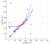
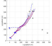
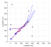
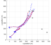
Figure 3: Exemplar outputs of the TPHD filter (top) and tagged PHD filter (bottom) at time steps 50 (left) and 70 (right), shown in a subregion of the surveillance area. The dashed blue lines represent the true trajectories. The blue squares and the numbers next to them denote the starting positions and starting times of different trajectories. There are four trajectories, two start at time step 1, close to each other, and end at time step 79. The other two start at time steps 5 and 10 and end at time steps 69 and 94, respectively. Black circles represent the current measurements. The TPHD filter is able to estimate the alive trajectories at each time step. The tagged PHD filter does not work well, as the estimator selects the highest peaks with distinct tags and there are two targets born from the same PHD component at the same time, which leads to track switching, false and missed targets. At time step 50, the tagged PHD filter estimates four trajectories, with one of length one in the birth location $\left[85,140\right]^{T}$. The tagged PHD filter at time step 70 estimates three trajectories, though one of them is no longer alive.

In the following, we evaluate the performance of the filters by Monte Carlo simulation with $N_{mc}=500$ runs. At each time step $k$, we measure the error between the set $\mathbf{X}_{a}^{k}$ of alive trajectories and its estimate $\mathbf{\hat{X}}_{a}^{k}$. In order to do so, we use the metric for sets of trajectories based on linear programming in [40] with parameters $p=2$, $c=10$ and $\gamma=1$, which we denote here as $d\left(\cdot,\cdot\right)$. In this case, $d^{2}\left(\cdot,\cdot\right)$ can be decomposed into the square costs: $c_{m}^{2}\left(\cdot,\cdot\right)$ for missed targets, $c_{f}^{2}\left(\cdot,\cdot\right)$ for false targets, $c_{l}^{2}\left(\cdot,\cdot\right)$ for the localisation error of properly detected targets, and $c_{t}^{2}\left(\cdot,\cdot\right)$ for track switches, as in performance evaluation in traditional multitarget tracking [41, Sec. 13.6]. That is, we have

$$d^{2}\left(\mathbf{X}_{a}^{k},\mathbf{\hat{X}}_{a}^{k}\right) =c_{l}^{2}\left(\mathbf{X}_{a}^{k},\mathbf{\hat{X}}_{a}^{k}\right)+c_{m}^{2}\left(\mathbf{X}_{a}^{k},\mathbf{\hat{X}}_{a}^{k}\right)$$

$$\quad+c_{f}^{2}\left(\mathbf{X}_{a}^{k},\mathbf{\hat{X}}_{a}^{k}\right)+c_{t}^{2}\left(\mathbf{X}_{a}^{k},\mathbf{\hat{X}}_{a}^{k}\right).$$ (42)

This decomposition is useful to analyse the performances of the filters, as done in this section. In our results, we only use the position elements to compute the error and normalise the error by the considered time window such that the squared error at time $k$ is $d^{2}\left(\mathbf{X}_{a}^{k},\mathbf{\hat{X}}_{a}^{k}\right)/k$. The root mean square (RMS) error at a given time step is calculated as

$$d\left(k\right) =\sqrt{\frac{1}{N_{mc}k}\sum_{i=1}^{N_{mc}}d^{2}\left(\mathbf{X}_{a}^{k},\mathbf{\hat{X}}_{a,i}^{k}\right)},$$ (43)

where $\mathbf{\hat{X}}_{a,i}^{k}$ is the estimate of the alive trajectories at time $k$ in the $i$th Monte Carlo run. In this scenario, the TPHD and TCPHD filters estimates do not have track switches and the resulting errors using $d\left(\mathbf{X}_{a}^{k},\mathbf{\hat{X}}_{a,i}^{k}\right)$ are the same as the errors computed by the sum of the generalised optimal sub-pattern assignment (GOSPA) metric ($\alpha=2$) [42] between the true targets and their estimates across all time steps. The tagged PHD and CPHD filters show track switches and therefore, the trajectory metric and GOSPA provide different errors.

The RMS trajectory errors for the algorithms are plotted in Figure 4. As expected, for the TPHD and TCPHD, increasing $L$ improves estimation performance and lowers the error. The TCPHD filter shows lower errors than the TPHD filter, except when targets disappear. The TCPHD filter also estimates the cardinality more accurately than the TPHD filter, except just after a target disappears, as can be seen in Figure 5. The tagged PHD and CPHD filters provide a considerably higher error, as track estimation is done in a manner that does not work well if two targets are born from the same PHD component at the same time.

In order to analyse the results more thoroughly, we make use of the metric decomposition indicated in (42). We compute the RMS costs in (42) at each time step normalised by $k$, as in (43). The results are shown in Figure 6. Tagged PHD and CPHD filters have a higher cost for missed targets and track switches than TPHD and TCPHD filters, as there are two targets born from the same PHD component and tagging does not work well in this case. We can see that increasing $L$ does not change the costs for missed and false targets and track switches for the trajectory algorithms, it mainly improves the localisation costs. We can see that the main advantage of using the TCPHD filter over the TPHD filter is the reduction of the number of missed targets. Both filters behave quite similarly in terms of localisation costs, missed targets and track switches. We can also see that the TCPHD filter has a higher cost for false targets than the PHD filter at time steps 70, 80 and 95, just after a target disappears.

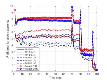
Figure 4: RMS trajectory metric error (43) of the alive trajectories for the TPHD/TCPHD filter and tagged PHD/CPHD filters. Filters based on sets of trajectories have a much higher performance than tagged filters. Increasing $L$ lowers the error.

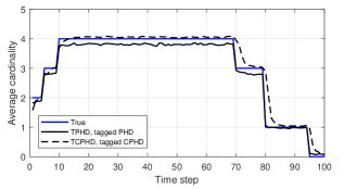
Figure 5: Estimated cardinality against time for the filters. CPHD-based filters estimate the cardinality more accurately except just after a target disappears.

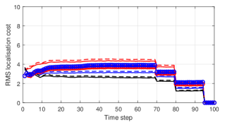
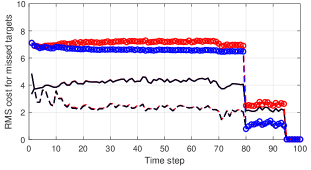
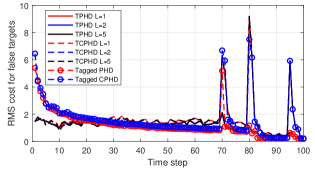
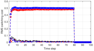
Figure 6: RMS costs for localisation errors for properly detected targets, missed targets, false targets and track switches for the alive trajectories at every time step. The scale of the $y$ axis changes in the figure for the switching cost. The RMS costs for missed targets and false targets do not change with the considered value of $L$. Increasing $L$, decreases the localisation cost for trajectory-based algorithms. TCPHD misses fewer targets than TPHD. Switching cost is negligible for TPHD/TCPHD filters. The tagged PHD and CPHD filters have a high cost for missed targets and show track switching.

The running times of our Matlab implementations of the filters in a computer with a 3.5 GHz Intel Xeon E5 processor are shown in Table I. The running times of the TCPHD filter are roughly 1 second longer than the TPHD for all values of $L$. For visualisation clarity, we have only shown performance results for $L\in\left\{1,2,5\right\}$ in Figures 4 and 6. For any $L\in\left\{10,20,30\right\}$, performance is similar and slightly better than for $L=5$. In particular, the RMS error (43) considering all time steps

$$d_{T}= \sqrt{1/N_{s}\cdot\sum_{k=1}^{N_{s}}d^{2}\left(k\right)}$$ (44)

using the trajectory metric is decreased from 4.68 (TPHD) and 3.90 (TCPHD) with $L=5$ to 4.66 (TPHD) and 3.87 (TCPHD) with $L\in\left\{10,20,30\right\}$. Tagged filters have a higher computational burden than TPHD and TCPHD with low $L$, due to the estimation process that links the current target state estimates with the previously estimated trajectories using the tags.

Table I: Running times of the algorithms in seconds

$L$	1	2	5	10	20	30
TPHD	1.1	1.1	1.2	1.7	3.4	6.0
TCPHD	2.0	2.0	2.1	2.6	4.3	6.9
Tagged PHD	2.2
Tagged CPHD	3.2

Table II: Error in alive trajectories averaged over all time steps for the trajectory metric (TM) and OSPA

	TPHD						TCPHD						Tagged PHD		Tagged CPHD
	TM/GOSPA			OSPA			TM/GOSPA			OSPA			TM	OSPA	TM	OSPA
$L$	1	2	5	1	2	5	1	2	5	1	2	5	-	-	-	-
No change	5.54	4.89	4.68	3.94	3.64	3.55	4.98	4.17	3.90	3.39	3.01	2.89	7.31	5.55	7.12	5.34
$\sigma^{2}=16$	9.31	8.50	8.04	5.83	5.40	5.17	8.27	8.39	7.88	5.61	5.14	4.87	8.95	6.37	8.94	6.29
$\sigma^{2}=1$	4.48	4.18	4.13	3.43	3.30	3.28	3.71	3.30	3.23	2.77	2.59	2.56	6.81	5.33	6.55	5.09
$\lambda_{c}=70$	5.61	4.98	4.78	4.01	3.72	3.63	5.09	4.33	4.07	3.50	3.15	3.03	7.27	5.53	7.05	5.30
$\lambda_{c}=30$	5.49	4.84	4.63	3.90	3.60	3.51	4.89	4.08	3.81	3.31	2.93	2.81	7.28	5.52	7.06	5.29
$p_{D}=0.99$	4.15	3.34	3.09	2.63	2.21	2.09	4.07	3.23	2.97	2.57	2.14	2.01	7.17	5.36	7.20	5.35
$p_{D}=0.85$	5.88	5.19	4.93	4.15	3.84	3.73	5.48	4.68	4.39	3.80	3.43	3.30	7.28	5.54	7.15	5.38
$p_{D}=0.75$	6.77	6.07	5.76	4.84	4.53	4.41	6.40	5.59	5.23	4.47	4.11	3.95	7.59	5.81	7.35	5.55
$p_{S}=0.95$	5.57	4.93	4.72	3.97	3.68	3.59	5.08	4.31	4.06	3.49	3.12	3.01	7.35	5.60	7.16	5.38
$w_{\beta,j}^{k}=0.05$	5.56	4.91	4.70	3.97	3.68	3.59	5.00	4.21	3.94	3.45	3.08	2.96	7.33	5.58	7.15	5.40

We also show the RMS error (44) for other simulation parameters in Table II. In this table, we also include results where $d\left(\cdot,\cdot\right)$ is the sum of the OSPA error [43, 44], with the same $p$ and $c$, between target states and their estimates at each time step. The trajectory metric and GOSPA return the same errors for TPHD/TCPHD filters, for all simulation parameters considered, which implies that the cost of track switches is negligible. Tagged filters show track switches so the trajectory metric and GOSPA do not coincide. GOSPA errors are not shown due to space constraints, but they are generally 0.02 lower than the trajectory metric error for the tagged filters. According to all the metrics and all scenarios, the TCPHD filter is the best performing filter, followed by the TPHD filter. For both filters, all metrics and scenarios, the error decreases as $L$ increases. The errors of the tagged filters are, in general, considerably higher than for the set of trajectories filters. As expected, performance improves for all filters if the probability of detection increases, clutter intensity decreases and the measurement noise variance decreases. We have also shown results with a different probability of survival and birth intensity to show that the results are consistent with different simulation parameters.

VIII Conclusions

In this paper we have developed the trajectory PHD and CPHD filters based on KLD minimisations and sets of trajectories. The TPHD and TCPHD filters propagate a Poisson multitrajectory density and an IID cluster multitrajectory density through the filtering recursion to make inference on the set of alive trajectories. The theory presented in this paper endows the PHD/CPHD filters with the capability of estimating trajectories from first principles, which can span their already widespread use to more applications where tracks are required.

We have also proposed a Gaussian mixture implementation of the filters. In particular, the parameter $L$ of the $L$-scan versions governs the accuracy of the estimation of past states of the trajectories. We have analysed the proposed filters in terms of localisation errors, missed targets, false targets and track switches, and also based on OSPA. Increasing $L$ mainly improves the localisation error of past states of the trajectory for both filters. In general, the TCPHD filter outperforms the TPHD filter, and both provide better trajectory estimates than the ones provided by tagging the PHD and CPHD filters.

Supplementary material of “Trajectory PHD and CPHD filters”

Appendix A

In this appendix, we indicate how to draw samples from an IID cluster trajectory RFS, which includes the Poisson trajectory RFS as a particular case. Given a single trajectory density $\breve{\nu}\left(\cdot\right)$, the probability that the trajectory starts at time $t$ and has duration $i$ is

$$P_{\breve{\nu}}\left(t,i\right)=\int\breve{\nu}\left(t,x^{1:i}\right)dx^{1:i}.$$ (45)

Given the start time $t$ and duration $i$, the density of the target states of the trajectory is

$$\breve{\nu}\left(x^{1:i}|t,i\right) =\frac{\breve{\nu}\left(t,x^{1:i}\right)}{P_{\breve{\nu}}\left(t,i\right)}.$$ (46)

Therefore, we can draw samples from an IID cluster trajectory RFS using (45) and (46), as indicated in Algorithm 3.

Algorithm 3 Sampling from an IID cluster multitrajectory density

Input: IID cluster multitrajectory density $\nu\left(\cdot\right)$.

Output: Sample $X\thicksim\nu\left(\cdot\right)$.

- Set $X=\emptyset$ and sample $n\thicksim\rho_{\nu}\left(\cdot\right)$.

for  $j=1$ to $n$  do

     - Sample $\left(t,i\right)\thicksim P_{\breve{\nu}}\left(\cdot\right)$ and $x^{1:i}\thicksim\breve{\nu}\left(\cdot|t,i\right)$, see (45) and (46).

     - Set $X\leftarrow X\cup\left\{\left(t,x^{1:i}\right)\right\}$.

end for

Appendix B

In this appendix we prove Theorem 4. A multitrajectory density $\pi\left(\cdot\right)$ can be written as [31]

$$\pi\left(\left\{X_{1},...,X_{n}\right\}\right)=\rho_{\pi}\left(n\right)n!\pi_{n}\left(X_{1},...,X_{n}\right)$$ (47)

where $\pi_{n}\left(\cdot\right)$ is a permutation invariant ordered trajectory density such that

$$\int\pi_{n}\left(X_{1},...,X_{n}\right)dX_{1:n} =1.$$

The marginal density of this density is written as

$$\tilde{\pi}_{n}\left(X\right) =\int\pi_{n}\left(X,X_{2}...,X_{n}\right)dX_{2:n}$$

$$=\frac{1}{\rho_{\pi}\left(n\right)n!}\int\pi\left(\left\{X,X_{2},...,X_{n}\right\}\right)dX_{2:n}.$$

Substituting (13) and (47) into (15), we get

$$\mathrm{D}\left(\pi\left\|\nu\right.\right) =\sum_{n=0}^{\infty}\rho_{\pi}\left(n\right)\log\frac{\rho_{\pi}\left(n\right)}{\rho_{\nu}\left(n\right)}$$

$$\quad+\sum_{n=0}^{\infty}\rho_{\pi}\left(n\right)\int\pi_{n}\left(X_{1},...,X_{n}\right)$$

$$\quad\times\log\frac{\pi_{n}\left(X_{1},...,X_{n}\right)}{\prod_{j=1}^{n}\breve{\nu}\left(X_{j}\right)}dX_{1:n}.$$ (48)

The objective is to find $\rho_{\nu}\left(\cdot\right)$ and $\breve{\nu}\left(\cdot\right)$ that minimise $\mathrm{D}\left(\pi\left\|\nu\right.\right)$. From KLD minimisation over discrete variables, $\rho_{\nu}\left(\cdot\right)=\rho_{\pi}\left(\cdot\right)$ minimises the KLD. Minimizing $\mathrm{D}\left(\pi\left\|\nu\right.\right)$ w.r.t. $\breve{\nu}\left(\cdot\right)$ is equivalent to minimising the functional

$$L\left[\breve{\nu}\right] =-\int\sum_{n=0}^{\infty}\rho_{\pi}\left(n\right)n\tilde{\pi}_{n}\left(X\right)\log\breve{\nu}\left(X\right)dX.$$

which is minimised by [29]

$$\breve{\nu}\left(X\right) =\frac{D_{\pi}\left(X\right)}{\sum_{n=0}^{\infty}\rho_{\pi}\left(n\right)n},$$

or equivalently, $D_{\nu}\left(\cdot\right)=D_{\pi}\left(\cdot\right)$.

Appendix C

In this appendix, we prove (18). The IID cluster multitrajectory density $\nu^{k}\left(\cdot\right)$ that minimises the KLD has the same cardinality distribution and PHD as $\pi^{k}\left(\cdot\right)$. The cardinality distribution of $\pi^{k}\left(\cdot\right)$ is such that $\rho_{\pi^{k}}\left(m\right)=1$, so we compute its PHD. The posterior can be written as [45, Eq. (12.91)]

$$\pi^{k}\left(\left\{X_{1},...,X_{m}\right\}\right) =\sum_{\sigma\in\Xi_{m}}\left[\prod_{i=1}^{m_{a}}\breve{a}_{i}\left(X_{\sigma_{i}}\right)\right]\left[\prod_{i=1}^{m_{d}}\breve{d}_{i}\left(X_{\sigma_{i+m_{a}}}\right)\right]$$ (49)

where $\Xi_{m}$ is the set that contains all permutations of $\left(1,...,m\right)$ and $\sigma_{i}$ is the $i$th component of $\sigma$.

Substituting (49) into (4), the PHD of the posterior is

$$D_{\pi^{k}}(X) =\sum_{n=0}^{\infty}\frac{1}{n!}\int\pi^{k}\left(\left\{X,X_{1},...,X_{n}\right\}\right)dX_{1:n}$$

$$=\sum_{i=1}^{m_{a}}\breve{a}_{i}\left(X\right)+\sum_{i=1}^{m_{d}}\breve{d}_{i}\left(X\right),$$

which is equal to $D_{\nu^{k}}(X)$. Then, using (14), we have that the single trajectory density $\breve{\nu}^{k}\left(\cdot\right)$ is

$$\breve{\nu}^{k}\left(X\right) =\frac{D_{\nu^{k}}(X)}{m}$$

$$=\frac{\sum_{i=1}^{m_{a}}\breve{a}_{i}\left(X\right)+\sum_{i=1}^{m_{d}}\breve{d}_{i}\left(X\right)}{m}.$$

A single trajectory with this density exists at the current time $k$ with probability $m_{a}/m$. As we have $m$ IID trajectories with this distribution, the number of alive trajectories follows the binomial distribution in (18).

Appendix D

In this appendix, we prove Theorem 9 (TCPHD update). The proof is quite similar to the CPHD update [16].

D-A Density of the measurement

As the current set of targets is an IID cluster with cardinality $\rho_{\omega^{k}}\left(\cdot\right)$ and PHD $D_{\omega_{T}^{k}}\left(\cdot\right)$, the density of the measurements, under Assumptions U1, U4 and U5, is the same as in the CPHD filter [16, Eq. (32)].

$$\ell^{k}\left(\mathbf{z}^{k}\right) =\left\langle\rho_{\omega^{k}},\Upsilon^{0}\left[D_{\omega_{\tau}^{k}},\mathbf{z}^{k}\right]\right\rangle\prod_{z\in\mathbf{z}^{k}}\breve{c}\left(z\right).$$ (50)

D-B Cardinality of the posterior

As the set of trajectories present at the current time has the same cardinality as the set of targets at the current time, the updated cardinality distribution is the same in both cases so the TCPHD cardinality update is the same as the CPHD filter cardinality update, which is given in (29).

D-C PHD of the posterior

The PHD of the posterior is

$$D_{\pi^{k}}(X)$$

$$\quad=\int\pi^{k}\left(\left\{X\right\}\cup\mathbf{X}\right)\delta\mathbf{X}$$

$$\quad=\frac{1}{\ell^{k}\left(\mathbf{z}^{k}\right)}\int\ell^{k}\left(\mathbf{z}^{k}\left|\tau^{k}\left(\left\{X\right\}\cup\mathbf{X}\right)\right.\right)\omega^{k}\left(\left\{X\right\}\cup\mathbf{X}\right)\delta\mathbf{X}$$

$$\quad=\frac{1}{\ell^{k}\left(\mathbf{z}^{k}\right)}\sum_{n=0}^{\infty}\left(n+1\right)\int\ell^{k}\left(\mathbf{z}^{k}|\tau^{k}\left(\left\{X,X_{1},...,X_{n}\right\}\right)\right)$$

$$\quad\times\rho_{\omega^{k}}\left(n+1\right)\breve{\omega}^{k}\left(X\right)\left[\prod_{j=1}^{n}\breve{\omega}^{k}\left(X_{j}\right)\right]dX_{1:n}.$$

We apply the decomposition [16, Eq. (14)]

$$\ell^{k}\left(\mathbf{z}^{k}\left|\tau^{k}\left(\left\{X\right\}\right)\cup\tau^{k}\left(\mathbf{X}\right)\right.\right)$$

$$\quad=\left(1-p_{D}\left(\tau^{k}\left(\left\{X\right\}\right)\right)\right)\ell^{k}\left(\mathbf{z}^{k}\left|\tau^{k}\left(\mathbf{X}\right)\right.\right)$$

$$\quad+p_{D}\left(\tau^{k}\left(\left\{X\right\}\right)\right)\sum_{z\in\mathbf{z}^{k}}l\left(z|\tau^{k}\left(\left\{X\right\}\right)\right)\ell^{k}\left(\mathbf{z}^{k}\setminus\left\{z\right\}\left|\tau^{k}\left(\mathbf{X}\right)\right.\right)$$

and obtain $D_{\pi^{k}}(t,x^{1:i})$

$$=\frac{\left(1-p_{D}\left(x^{i}\right)\right)\breve{\omega}^{k}\left(t,x^{1:i}\right)}{\ell^{k}\left(\mathbf{z}^{k}\right)}\sum_{n=0}^{\infty}\left(n+1\right)\rho_{\omega^{k}}\left(n+1\right)$$

$$\quad\times\int\ell^{k}\left(\mathbf{z}^{k}|\tau^{k}\left(\left\{X_{1},...,X_{n}\right\}\right)\right)\left[\prod_{j=1}^{n}\breve{\omega}^{k}\left(X_{j}\right)\right]dX_{1:n}$$

$$\quad+\frac{p_{D}\left(x^{i}\right)\breve{\omega}^{k}\left(t,x^{1:i}\right)}{\ell^{k}\left(\mathbf{z}^{k}\right)}\sum_{z\in\mathbf{z}^{k}}l\left(z|x^{i}\right)\sum_{n=0}^{\infty}\left(n+1\right)\rho_{\omega^{k}}\left(n+1\right)$$

$$\quad\times\int\ell^{k}\left(\mathbf{z}^{k}\setminus\left\{z\right\}\left|\tau^{k}\left(\left\{X_{1},...,X_{n}\right\}\right)\right.\right)\left[\prod_{j=1}^{n}\breve{\omega}^{k}\left(X_{j}\right)\right]dX_{1:n}$$

$$=\frac{\left(1-p_{D}\left(x^{i}\right)\right)\breve{\omega}^{k}\left(t,x^{1:i}\right)}{\ell^{k}\left(\mathbf{z}^{k}\right)}\sum_{n=0}^{\infty}\left(n+1\right)\rho_{\omega^{k}}\left(n+1\right)$$

$$\quad\times\int\ell^{k}\left(\mathbf{z}^{k}|\left\{x_{1},...,x_{n}\right\}\right)\left[\prod_{j=1}^{n}\breve{\omega}_{\tau}^{k}\left(x_{j}\right)\right]dx_{1:n}$$

$$\quad+\frac{p_{D}\left(x^{i}\right)\breve{\omega}^{k}\left(t,x^{1:i}\right)}{\ell^{k}\left(\mathbf{z}^{k}\right)}\sum_{z\in\mathbf{z}^{k}}l\left(z|x^{i}\right)\sum_{n=0}^{\infty}\left(n+1\right)\rho_{\omega^{k}}\left(n+1\right)$$

$$\quad\times\int\ell^{k}\left(\mathbf{z}^{k}\setminus\left\{z\right\}\left|\left\{x_{1},...,x_{n}\right\}\right.\right)\left[\prod_{j=1}^{n}\breve{\omega}_{\tau}^{k}\left(x_{j}\right)\right]dx_{1:n}.$$ (51)

From [16, Eq. (39)], we know that

$$\sum_{n=0}^{\infty}\left(n+1\right)\rho_{\omega^{k}}\left(n+1\right)$$

$$\quad\times\int\ell^{k}\left(\mathbf{z}^{k}|\left\{x_{1},...,x_{n}\right\}\right)\left[\prod_{j=1}^{n}\breve{\omega}_{\tau}^{k}\left(x_{j}\right)\right]dx_{1:n}$$

$$\quad=\int D_{\omega_{\tau}^{k}}(x)dx\left\langle\rho_{\omega^{k}},\Upsilon^{1}\left[D_{\omega_{\tau}^{k}},\mathbf{z}^{k}\right]\right\rangle\prod_{z\in\mathbf{z}^{k}}\breve{c}\left(z\right).$$ (52)

Substituting (50) and (52) into the first and second term of (51) completes the proof of (30).

Appendix E

In this appendix, we prove Theorem 8 (TCPHD prediction). We proceed to calculate the cardinality and PHD of the predicted multitrajectory density. As in the CPHD filter, the assumptions of the TCPHD filter prediction (P1, P4, P5) are similar to the TCPHD filter update (U1, U4, U5) so the proof of the TCPHD filter update, which is given in Appendix D, is useful for the TCPHD filter prediction, as in the CPHD filter [16].

E-A Cardinality

The cardinality distribution of the predicted multitrajectory density for alive targets is analogous to the cardinality distribution $\rho_{\ell^{k}}\left(\cdot\right)$ of the measurement, which can be calculated from (50) in the same way as in [16, Sec. V.C]. The result is

$$\rho_{\ell^{k}}\left(m\right) =\sum_{j=0}^{m}\rho_{c}\left(m-j\right)\sum_{n=j}^{\infty}\left(\begin{array}[]{c}n\\ j\end{array}\right)\rho_{\omega^{k}}\left(n\right)$$

$$\quad\times\frac{\left[\int\left(1-p_{D}(x)\right)D_{\omega_{\tau}^{k}}(x)dx\right]^{n-j}}{\left[\int D_{\omega_{\tau}^{k}}(x)dx\right]^{n}}$$

$$\quad\times\left[\int p_{D}\left(x\right)D_{\omega_{\tau}^{k}}(x)dx\right]^{j}.$$

By changing $\rho_{c}\left(\cdot\right)$, $p_{D}\left(\cdot\right)$ and $\omega^{k}\left(\cdot\right)$ for $\rho_{\beta^{k}}\left(\cdot\right)$, $p_{S}\left(\cdot\right)$ and $\pi{}^{k}\left(\cdot\right)$, respectively, we obtain (28).

E-B PHD

The result for the PHD of the TCPHD prediction, which is the same as for the TPHD prediction, see (21), can be established directly based on thinning, displacement and superposition of point processes, as in the CPHD filter for targets [16]. Nevertheless, for completeness, we provide more details regarding its calculation here.

We have a multitrajectory density $\pi^{k-1}\left(\cdot\right)$ with a PHD $D_{\pi_{k-1}}\left(\cdot\right)$ and we want to compute the PHD of the multitrajectory density $\omega^{k}\left(\cdot\right)$, which is $D_{\omega^{k}}\left(\cdot\right)$. We first compute the PHD of $\xi^{k}\left(\cdot\right)$, which represents the multitrajectory density of the surviving trajectories and is given by

$$\xi^{k}\left(\mathbf{X}\right) =\int f_{s}\left(\mathbf{X}|\mathbf{Y}\right)\pi^{k-1}\left(\mathbf{Y}\right)\delta\mathbf{Y}$$ (53)

where $f_{s}\left(\cdot|\cdot\right)$ is the transition multitrajectory density for surviving trajectories. We proceed to explain a decomposition of $f_{s}\left(\cdot|\cdot\right)$, which will be useful for the proof.

We first write the probability of survival and single trajectory transition density for alive trajectories at time $k$ as a function of trajectories. These correspond to

$$p^{\prime}_{S}\left(t,x^{1:i}\right) =p_{S}\left(x^{i}\right)$$ (54)

$$g^{\prime}\left(t,x^{1:i}|t^{\prime},z^{1:i^{\prime}}\right) =\delta\left[t-t^{\prime}\right]g\left(x^{i}|z^{i^{\prime}}\right)\delta\left(x^{1:i-1}-z^{1:i^{\prime}}\right)$$ (55)

where $t+i-1=k$ and $t^{\prime}+i^{\prime}-1=k-1$, otherwise, $p^{\prime}_{S}\left(\cdot\right)$ and $g^{\prime}\left(\cdot|\cdot\right)$ are zero. Also, $\delta\left[\cdot\right]$ and $\delta\left(\cdot\right)$ denote Kronecker and Dirac delta, respectively.

We use the following decomposition for the transition density of surviving trajectories

$$f_{s}\left(\left\{X\right\}\cup\mathbf{X}|\mathbf{Y}\right) =\sum_{Y\in\mathbf{Y}}g^{\prime}\left(X|Y\right)p^{\prime}_{S}\left(Y\right)f_{s}\left(\mathbf{X}|\mathbf{Y}\setminus\left\{Y\right\}\right).$$

Note that this decomposition results from the fact that given the surviving trajectories $\left\{X\right\}\cup\mathbf{X}$, trajectory $X$ must have survived from a trajectory $Y$ that belongs to $\mathbf{Y}$ and the rest of the surviving trajectories $\mathbf{X}$ have survived from the rest of the trajectories at the previous time step $\mathbf{Y}\setminus\left\{Y\right\}$.

The PHD of the surviving trajectories is obtained by substituting (53) into (4)

$$D_{\xi^{k}}\left(X\right) =\int\xi^{k}\left(\mathbf{X}\cup\left\{X\right\}\right)\delta\mathbf{X}$$

$$=\int\left[\int f_{s}\left(\left\{X\right\}\cup\mathbf{X}|\mathbf{Y}\right)\delta\mathbf{X}\right]\pi^{k-1}\left(\mathbf{Y}\right)\delta\mathbf{Y}.$$ (56)

We simplify the inner integral in (56) as

$$\int f_{s}\left(\left\{X\right\}\cup\mathbf{X}|\mathbf{Y}\right)\delta\mathbf{X}$$

$$=\int\sum_{Y\in\mathbf{Y}}g^{\prime}\left(X|Y\right)p^{\prime}_{S}\left(Y\right)f_{s}\left(\mathbf{X}|\mathbf{Y}\setminus\left\{Y\right\}\right)\delta\mathbf{X}$$

$$=\sum_{Y\in\mathbf{Y}}g^{\prime}\left(X|Y\right)p^{\prime}_{S}\left(Y\right).$$

Substituting this equation into (56) and applying Campbell’s theorem [1, Sec. 4.2.12]

$$D_{\xi^{k}}\left(X\right) =\int\left(\sum_{Y\in\mathbf{Y}}g^{\prime}\left(X|Y\right)p^{\prime}_{S}\left(Y\right)\right)\pi^{k-1}\left(\mathbf{Y}\right)\delta\mathbf{Y}$$

$$=\int g^{\prime}\left(X|Y\right)p^{\prime}_{S}\left(Y\right)D_{\pi^{k-1}}\left(Y\right)dY.$$ (57)

Substituting (54) and (55) into (57) yields $D_{\xi^{k}}\left(\cdot\right)$ in (21). By the superposition theorem of point processes [46], the PHD of $\omega^{k}\left(\cdot\right)$ is the sum of the PHDs of the surviving trajectories, which is given by $D_{\xi^{k}}\left(\cdot\right)$, and the PHD of the new born trajectories, which is given by $D_{\beta^{k}}\left(\cdot\right)$. Therefore, the TCPHD prediction equation for the PHD is the same as for the TPHD filter, see (21).

References

- [1] R. P. S. Mahler, Advances in Statistical Multisource-Multitarget Information Fusion. Artech House, 2014.
- [2] K. Granström, C. Lundquist, and O. Orguner, “Extended target tracking using a Gaussian-mixture PHD filter,” IEEE Transactions on Aerospace and Electronic Systems, vol. 48, no. 4, pp. 3268–3286, Oct. 2012.
- [3] B.-N. Vo and W.-K. Ma, “The Gaussian mixture probability hypothesis density filter,” IEEE Transactions on Signal Processing, vol. 54, no. 11, pp. 4091–4104, Nov. 2006.
- [4] C. Lundquist, K. Granström, and U. Orguner, “An extended target CPHD filter and a gamma Gaussian inverse Wishart implementation,” IEEE Journal of Selected Topics in Signal Processing, vol. 7, no. 3, pp. 472–483, June 2013.
- [5] B.-T. Vo, B.-N. Vo, and A. Cantoni, “Analytic implementations of the cardinalized probability hypothesis density filter,” IEEE Transactions on Signal Processing, vol. 55, no. 7, pp. 3553–3567, July 2007.
- [6] N. Whiteley, S. Singh, and S. Godsill, “Auxiliary particle implementation of probability hypothesis density filter,” IEEE Transactions on Aerospace and Electronic Systems, vol. 46, no. 3, pp. 1437–1454, July 2010.
- [7] O. Erdinc, P. Willett, and Y. Bar-Shalom, “The bin-occupancy filter and its connection to the PHD filters,” IEEE Transactions on Signal Processing, vol. 57, no. 11, pp. 4232–4246, Nov. 2009.
- [8] M. Üney, D. E. Clark, and S. J. Julier, “Distributed fusion of PHD filters via exponential mixture densities,” IEEE Journal of Selected Topics in Signal Processing, vol. 7, no. 3, pp. 521–531, June 2013.
- [9] G. Battistelli, L. Chisci, C. Fantacci, A. Farina, and A. Graziano, “Consensus CPHD filter for distributed multitarget tracking,” IEEE Journal of Selected Topics in Signal Processing, vol. 7, no. 3, pp. 508–520, June 2013.
- [10] C. S. Lee, S. Nagappa, N. Palomeras, D. Clark, and J. Salvi, “SLAM with SC-PHD filters: An underwater vehicle application,” IEEE Robotics & Automation Magazine, vol. 21, no. 2, pp. 38–45, June 2014.
- [11] J. Mullane, B.-N. Vo, M. D. Adams, and B.-T. Vo, “A random-finite-set approach to Bayesian SLAM,” IEEE Transactions on Robotics, vol. 27, no. 2, pp. 268–282, April 2011.
- [12] E. Maggio, M. Taj, and A. Cavallaro, “Efficient multitarget visual tracking using random finite sets,” IEEE Transactions on Circuits and Systems for Video Technology, vol. 18, no. 8, pp. 1016–1027, Aug. 2008.
- [13] T. M. Wood, C. A. Yates, D. A. Wilkinson, and G. Rosser, “Simplified multitarget tracking using the PHD filter for microscopic video data,” IEEE Transactions on Circuits and Systems for Video Technology, vol. 22, no. 5, pp. 702–713, May 2012.
- [14] C. Lundquist, L. Hammarstrand, and F. Gustafsson, “Road intensity based mapping using radar measurements with a probability hypothesis density filter,” IEEE Transactions on Signal Processing, vol. 59, no. 4, pp. 1397–1408, April 2011.
- [15] B. Ristic, B.-N. Vo, and D. Clark, “A note on the reward function for PHD filters with sensor control,” IEEE Transactions on Aerospace and Electronic Systems, vol. 47, no. 2, pp. 1521–1529, April 2011.
- [16] A. F. García-Fernández and B.-N. Vo, “Derivation of the PHD and CPHD filters based on direct Kullback-Leibler divergence minimization,” IEEE Transactions on Signal Processing, vol. 63, no. 21, pp. 5812–5820, Nov. 2015.
- [17] D. Franken, M. Schmidt, and M. Ulmke, “"Spooky action at a distance" in the cardinalized probability hypothesis density filter,” IEEE Transactions on Aerospace and Electronic Systems, vol. 45, no. 4, pp. 1657–1664, Oct. 2009.
- [18] N. Nadarajah, T. Kirubarajan, T. Lang, M. McDonald, and K. Punithakumar, “Multitarget tracking using probability hypothesis density smoothing,” IEEE Transactions on Aerospace and Electronic Systems, vol. 47, no. 4, pp. 2344–2360, Oct. 2011.
- [19] S. Nagappa, E. D. Delande, D. E. Clark, and J. Houssineau, “A tractable forward-backward CPHD smoother,” IEEE Transactions on Aerospace and Electronic Systems, vol. 53, no. 1, pp. 201–217, Feb. 2017.
- [20] L. Lin, Y. Bar-Shalom, and T. Kirubarajan, “Track labeling and PHD filter for multitarget tracking,” IEEE Transactions on Aerospace and Electronic Systems, vol. 42, no. 3, pp. 778–795, July 2006.
- [21] K. Panta, B.-N. Vo, and S. Singh, “Novel data association schemes for the probability hypothesis density filter,” IEEE Transactions on Aerospace and Electronic Systems, vol. 43, no. 2, pp. 556–570, April 2007.
- [22] K. Panta, D. Clark, and B.-N. Vo, “Data association and track management for the Gaussian mixture probability hypothesis density filter,” IEEE Transactions on Aerospace and Electronic Systems, vol. 45, no. 3, pp. 1003–1016, July 2009.
- [23] E. Pollard, B. Pannetier, and M. Rombaut, “Hybrid algorithms for multitarget tracking using MHT and GM-CPHD,” IEEE Transactions on Aerospace and Electronic Systems, vol. 47, no. 2, pp. 832–847, April 2011.
- [24] Z. Lu, W. Hu, Y. Liu, and T. Kirubarajan, “A new cardinalized probability hypothesis density filter with efficient track continuity and extraction,” in 21st International Conference on Information Fusion, 2018.
- [25] Z. Lu, W. Hu, and T. Kirubarajan, “Labeled random finite sets with moment approximation,” IEEE Transactions on Signal Processing, vol. 65, no. 13, pp. 3384–3398, July 2017.
- [26] A. F. García-Fernández, J. Grajal, and M. R. Morelande, “Two-layer particle filter for multiple target detection and tracking,” IEEE Transactions on Aerospace and Electronic Systems, vol. 49, no. 3, pp. 1569–1588, July 2013.
- [27] B. T. Vo and B. N. Vo, “Labeled random finite sets and multi-object conjugate priors,” IEEE Transactions on Signal Processing, vol. 61, no. 13, pp. 3460–3475, July 2013.
- [28] A. F. García-Fernández, L. Svensson, and M. R. Morelande, “Multiple target tracking based on sets of trajectories,” accepted for publication in IEEE Transactions on Aerospace and Electronic Systems, 2019. [Online]. Available: https://arxiv.org/abs/1605.08163
- [29] A. F. García-Fernández and L. Svensson, “Trajectory probability hypothesis density filter,” in 21st International Conference on Information Fusion, 2018.
- [30] L. Svensson and M. Morelande, “Target tracking based on estimation of sets of trajectories,” in 17th International Conference on Information Fusion, 2014.
- [31] R. P. S. Mahler, “Multitarget Bayes filtering via first-order multitarget moments,” IEEE Transactions on Aerospace and Electronic Systems, vol. 39, no. 4, pp. 1152–1178, Oct. 2003.
- [32] J. L. Williams, “An efficient, variational approximation of the best fitting multi-Bernoulli filter,” IEEE Transactions on Signal Processing, vol. 63, no. 1, pp. 258–273, Jan. 2015.
- [33] A. Papoulis and S. U. Pillai, Probability, Random Variables and Stochastic Processes. McGraw-Hill, 2002.
- [34] K. Granström, L. Svensson, Y. Xia, J. L. Williams, and A. F. García-Fernández, “Poisson multi-Bernoulli mixture trackers: continuity through random finite sets of trajectories,” in 21st International Conference on Information Fusion, 2018.
- [35] S. Särkkä, Bayesian Filtering and Smoothing. Cambridge University Press, 2013.
- [36] D. Salmond, “Mixture reduction algorithms for point and extended object tracking in clutter,” IEEE Transactions on Aerospace and Electronic Systems, vol. 45, no. 2, pp. 667–686, April 2009.
- [37] W. Koch and F. Govaers, “On accumulated state densities with applications to out-of-sequence measurement processing,” IEEE Transactions on Aerospace and Electronic Systems, vol. 47, no. 4, pp. 2766–2778, 2011.
- [38] H. Oruç and H. K. Akmaz, “Symmetric functions and the Vandermonde matrix,” Journal of Computational and Applied Mathematics, vol. 172, no. 1, pp. 49–64, Nov. 2004.
- [39] A. F. García-Fernández, L. Svensson, M. R. Morelande, and S. Särkkä, “Posterior linearization filter: principles and implementation using sigma points,” IEEE Transactions on Signal Processing, vol. 63, no. 20, pp. 5561–5573, Oct. 2015.
- [40] A. S. Rahmathullah, A. F. García-Fernández, and L. Svensson, “A metric on the space of finite sets of trajectories for evaluation of multi-target tracking algorithms,” 2016. [Online]. Available: http://arxiv.org/abs/1605.01177
- [41] S. Blackman and R. Popoli, Design and Analysis of Modern Tracking Systems. Artech House, 1999.
- [42] A. S. Rahmathullah, A. F. García-Fernández, and L. Svensson, “Generalized optimal sub-pattern assignment metric,” in 20th International Conference on Information Fusion, 2017.
- [43] D. Schuhmacher and A. Xia, “A new metric between distributions of point processes,” vol. 40, no. 3, pp. 651–672, Sep. 2008.
- [44] D. Schuhmacher, B.-T. Vo, and B.-N. Vo, “A consistent metric for performance evaluation of multi-object filters,” IEEE Transactions on Signal Processing, vol. 56, no. 8, pp. 3447–3457, Aug. 2008.
- [45] R. P. S. Mahler, Statistical Multisource-Multitarget Information Fusion. Artech House, 2007.
- [46] D. Stoyan, W. S. Kendall, and J. Mecke, Stochastic geometry and its applications. John Wiley & Sons, 1995.