High-frequency breakdown of the integer QHE in GaAs/AlGaAs heterojunctions

Abstract

The integer quantum Hall effect is a well-studied phenomenon at frequencies below about 100 Hz. The plateaus in high-frequency Hall conductivity were experimentally proven to retain up to 33 GHz, but the behavior at higher frequencies has remained largely unexplored. Using continuous wave THz spectroscopy, the complex Hall conductivity of GaAs/AlGaAs heterojunctions was studied in the range of 69–1100 GHz. Above 100 GHz, the quantum plateaus are strongly smeared out and replaced by weak quantum oscillations in the real part of the conductivity. The amplitude of the oscillations decreases with increasing frequency. Near 1 THz, the Hall conductivity does not reveal any features related to the filling of Landau levels. Similar oscillations are observed in the imaginary part as well, this effect has no analogy at zero frequency. This experimental picture is in disagreement with existing theoretical considerations of the high-frequency quantum Hall effect.

I Introduction

The discovery of the integer quantum Hall effect (IQHE)Klitzing et al. (1980) has attracted much interest in scientific community. The vast majority of experimental and theoretical investigations have been devoted to the study of the QHE at frequencies below 100 Hz, and in this range the phenomenon of Hall quantization has been studied very extensively. In experiments on QHE it is more convenient to apply an alternating current, rather than a direct current. At several Hertz $\sigma_{xy}(\omega)$ is indistinguishable from the DC Hall conductivity. Measurable frequency dependence can be detected when $\omega$ is increased up to the microwave range. In this range the standard contact techniques become inapplicable and high-frequency Hall conductivity is be studied using the interaction of electromagnetic waves with a two-dimensional electron gas (2DEG). Kuchar et al.Kuchar et al. (1986) used a crossed waveguide setup to observe Hall quantization at 33 GHz. Galchenkov et al.Galchenkov et al. (1987) used a circular waveguide to study the evolution of the Hall plateaus in the 24–70 GHz range. A review of experiments on the longitudinal conductivity $\sigma_{xx}(\omega)$ below 20 GHz can be found in Ref. [Hohls et al., 2002].

Further frequency increases can be achieved in quasi-optical spectrometers, suitable for measurements in the range of 100–1000 GHz. In the case of a thin conducting film, the Hall conductivity is directly related to the Faraday rotation angleVolkov and Mikhailov (1985). Recent experimental works Shimano et al. (2013); Okada et al. (2016); Wu et al. (2016); Dziom et al. (2017a) on the observation of the quantized Faraday rotation in novel materials have inspired a development of theories for a non-linear Hall response Tse (2016); Lee and Tse (2017). A linear high-frequency Hall response is far from being completely understood for systems with parabolic electron bands (AlGaAs, Si, Ge). Experimentally, the Hall effect in the THz range was observed in GaAs/AlGaAs heterojunctions Ikebe et al. (2010); Stier et al. (2015) and in Ge quantum wells Failla et al. (2016). The high-frequency data in Refs. [Ikebe et al., 2010; Stier et al., 2015; Failla et al., 2016] do not demonstrate quantum plateaus that would be comparable with corresponding DC data. In Ref. [Stier et al., 2015] the experiment was conducted at two frequencies (2.52 and 3.14 THz), using an optically pumped molecular gas laser. In Refs. [Ikebe et al., 2010,Failla et al., 2016] the Hall conductivity was measured using time-domain spectroscopy (TDS). In principle, TDS allows the Hall conductivity to be obtained at fixed frequencies, but the authors present the data averaged over a wide spectral range. Due to this averaging, information about the frequency dependence of the Hall conductivity was lost. Thus, the question, of how the static QHE transforms into a dynamic one, remains unresolved.

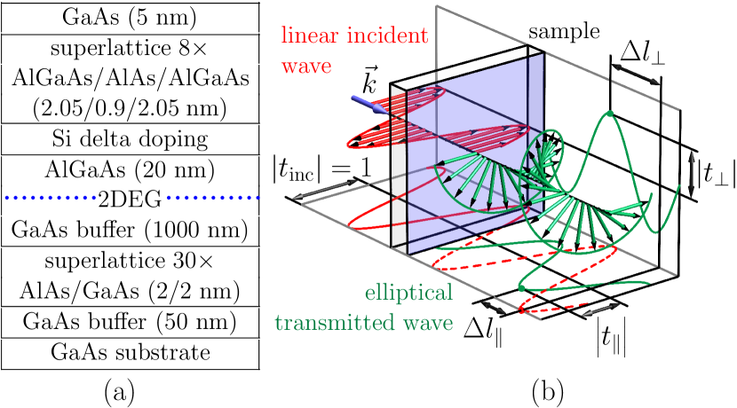
Figure 1: (a) Detailed structure of GaAs/AlGaAs heterojunctions. The aluminum fraction in Al_xGa_1-xAs is $x=31.35$%. The samples #1 and #2 differ by the amount of silicon in the doping layer (Tab. 1). (b) Transmission spectroscopy of a two-dimensional electron gas. The linearly polarized incident wave becomes elliptically polarized upon passing through the electron gas in a magnetic field. Using a polarizer (not shown), transmission amplitudes of the linear components were measured along initial ($t_{\parallel}$) and perpendicular ($t_{\perp}$) directions. A second reference beam, schematically shown by the red dashed line, was used to determine the phase shift $\Delta l$ produced by the sample. The knowledge of two complex transmission coefficients $t_{\parallel}=\left|t_{\parallel}\right|e^{\imath k\Delta l_{\parallel}}$ and $t_{\perp}=\left|t_{\perp}\right|e^{\imath k\Delta l_{\perp}}$ is sufficient to calculate the high-frequency complex Hall conductivity without additional model assumptions.

In order to study the evolution of the quantum Hall plateaus with respect to frequency, a series of experiments were conducted on MBE-grown GaAs/AlGaAs heterojunctions, one of the most suitable system to investigate the DC QHE. The results of the crossed-waveguide method were reproduced Kuchar et al. (1986); Galchenkov et al. (1987) and a QHE plateau was observed at 69 GHz. Above 100 GHz the plateaus were replaced by oscillations that disappeared completely as the frequency approached 1 THz.

II Samples and experimental technique

Table 1: Parameters of GaAs/AlGaAs heterostructures at $T=1.9$ K. $n_{\text{2D}}$: two-dimensional density, $\mu$: mobility, $\tau$: relaxation time, $m$: cyclotron mass, size: dimensions of the substrate. The superscripts “DC” and “THz” denote the quantities, independently obtained in DC and spectroscopic experiments, respectively.

	Sample #1	Sample #2
$n_{\text{2D}}^{\text{DC}}$(cm-2)	$(2.3\pm 0.2)\times 10^{11}$	$(3.6\pm 0.3)\times 10^{11}$
$n_{\text{2D}}^{\text{THz}}$(cm-2)	$(2.4\pm 0.2)\times 10^{11}$	$(3.9\pm 0.8)\times 10^{11}$
$\mu^{\text{DC}}$(cm2/(V$\cdot$s))	$(1.0\pm 0.1)\times 10^{5}$	$(3.2\pm 0.5)\times 10^{5}$
$\mu^{\text{THz}}$(cm2/(V$\cdot$s))	$(1.1\pm 0.1)\times 10^{5}$	$(2.5\pm 0.5)\times 10^{5}$
$\tau$(ps)	$4.5\pm 0.5$	$10\pm 2$
$m/m_{0}$	$0.070\pm 0.001$	$0.070\pm 0.002$
size (mm3)	10$\times$10$\times$0.660	5$\times$5$\times$0.367

The experimental data, presented in this paper, have been obtained on two GaAs/AlGaAs heterojunctions, grown by molecular beam epitaxy (see Fig. 1(a)). Characteristic parameters of the samples, obtained in DC and spectroscopic experiments at 1.9 K, are given in Tab. 1. Sample #1 had a reduced silicon delta doping level in comparison with sample #2, which led to a lower electron density and a shorter relaxation time. Insulating GaAs, used as a substrate, was transparent to the radiation in the full range of the spectrometer. The substrate was characterized by a dielectric constant $\varepsilon=12$ with a negligible frequency dependence. Indium electrical contacts Sebestyen (1982); Lakhani (1984), placed in the corners and the center of the sides, were prepared on each sample by baking at 400^∘C in a reducing atmosphere (Ar+4%H). All spectroscopic experiments were accompanied by simultaneous measurements of resistances $R_{xx}$ and $R_{xy}$ using lock-in techniques; typical values of the applied current were $I\approx 1\,\mu$A. The application of the relatively high current without non-linear effects was possible because of large dimensions of the samples in comparison with standard Hall bars, see Tab. 1. During the experiments the sample was placed into a superconducting magnet with optical windows, made of $50\,\mu$m mylar films. The sample volume was filled with liquid helium and pumped down to maintain the temperature of the sample at 1.9 K.

Heterostructures including mixed Al_xGa_1-xAs layers (Fig. 1(a)) are known to demonstrate a strong effect of persistent photoconductivity Baba et al. (1983). For samples cooled in the dark the subsequent illumination with visible light leads to an increase of the electron density Nathan (1986). The photo-induced charge carriers persist in the sample even after the switching off of the light and they may create an additional conductive channel parallel to the 2D electrons. In experiments on illuminated samples #1 and #2 the longitudinal DC resistance $R_{xx}$ acquired non-zero values at integer filling factors and the shape of Hall plateaus became distorted after illumination. In order to avoid the persistent photoconductivity effects the optical windows were constantly covered by black paper that blocked visible light. All data presented in this work were obtained on samples in the dark.

The high-frequency Hall conductivity of the two-dimensional electron gas was measured in the range of 69-1100 GHz using a two-beam Mach-Zehnder interferometer. Backward wave oscillators (BWOs) produced a continuous monochromatic wave that was guided in free space using dielectric lenses, metallic mirrors and free-standing wire-grid polarizers. A quasi-parallel incident beam was focused on a sample by a lens with a diameter of 50 mm and a focal distance of 140 mm. The transmitted wave passed through a similar lens to restore a quasi-parallel beam. The intensity of the transmitted beam was measured by a 4.2 K helium cooled Si bolometer.

Upon passing through the sample, the linearly polarized wave became elliptically polarized, see Fig. 1(b). First, a linear component with the same polarization as in the incident wave was filtered by a wire-grid polarizer. The intensity of this component with the sample in the beam divided by the intensity without the sample gave the absolute value of the complex parallel transmission $\left|t_{\parallel}\right|^{2}$. The phase shift $\Delta l_{\parallel}$ was measured using a reference beam to obtain the complex parallel coefficient as $t_{\parallel}=\left|t_{\parallel}\right|e^{\imath k\Delta l_{\parallel}}$, where $k=\omega/c$ is the wave vector. The polarizer was then rotated by $90^{\circ}$ and the procedure was repeated to obtain a complex crossed transmission coefficient $t_{\perp}=\left|t_{\perp}\right|e^{\imath k\Delta l_{\perp}}$.

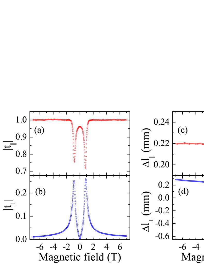
Figure 2: Field dependence of the transmission coefficients for sample #1 (Tab. 1) at 332 GHz. Cyclotron resonance is observed at $\pm 0.83$ T as a dip in the parallel amplitude (a) and a peak in the crossed amplitude (b). The sign change of the external magnetic field does not affect the parallel transmission ($t_{\parallel}(B)=t_{\parallel}(-B)$), while the complex crossed coefficient changes sign ($t_{\perp}(B)=-t_{\perp}(-B)$). As a result, the parallel phase shift generated by the sample is an even function of magnetic field (c), and the values of the crossed phase shift differ by half a wavelength (d). The panel (e) shows $\left|t_{\perp}\right|$ near a wide plateau in DC Hall conductance.

In order to obtain the Hall conductivity as a function of the magnetic field, the transmission coefficients were measured at fixed frequencies (Fig. 2). The frequency generated by the BWO was controlled by an accelerating voltage and could be set to any value within a certain range. Acting as a Fabry-Pérot resonator, the dielectric substrate produced regular oscillations in the transmission spectra (see the upper inset in Fig. 3). The frequencies $f_{z}$, at which the transmission was maximal, were determined by the relation $\sqrt{\varepsilon}ka=\pi z$, where $z$ is an integer. In the framework of a matrix formalism Berreman (1972), the substrate is described by a transfer matrix $M$ that connects electromagnetic (EM) fields at the opposite surfaces. At frequencies $f_{z}$, the transfer matrix of a non-absorbing dielectric slab degenerates into an identity matrix: $M=(-1)^{z}I$. At these frequencies the substrate virtually “disappears”, as it simply duplicates the EM field at its surfaces. In transmission coefficients the substrate causes only a phase shift that is equal to the thickness and a sign change, if $z$ is odd. For sample #1 ($\varepsilon=12$, $a=0.66$ mm), the frequencies $f_{z}$ were multiples of 67 GHz. Measuring at one of the transmission maxima allows a higher signal to be obtained, all else being equal. For this reason, most of the measurements at fixed frequencies $f$, presented in this work, were carried out at $f\approx f_{z}$.

The lowest frequency at which the quasi-optical method produces reliable results, is determined by the sample dimensions. The size of the focal spot can be estimated as $f\lambda/D$, where $f=140$ mm is the focal distance, $D=50$ mm is the diameter of the lens and $\lambda$ is the radiation wavelength. The measured transmission coefficient starts to be affected by diffraction corrections when the focal spot is comparable with the sample dimensions. Therefore, in case of larger sample #1 (see Tab. 1) the spectroscopic measurements could be extended down to frequencies below 100 GHz.

III Data processing

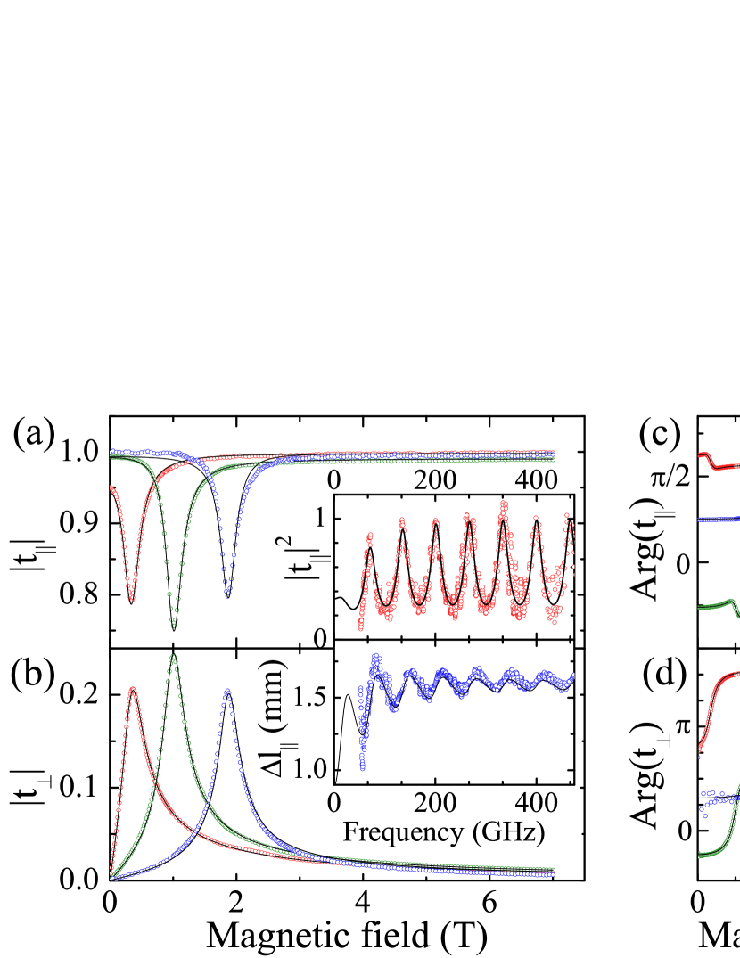
Figure 3: Symmetrized transmission coefficients for sample #1 at frequencies 134 (red), 401 (green) and 730 GHz (blue) as a function of external magnetic field. The parallel transmission in the zero field is shown as a function of frequency in the inset. The black solid lines represent classical Drude fits.

Knowing the two complex coefficients $t_{\parallel}$ and $t_{\perp}$, the complex Hall conductivity can be calculated at frequency $\omega$ as in Ref. [Dziom et al., 2017b]:

$$\sigma_{xy}=\frac{2\sqrt{\varepsilon}e^{-\imath ka}t_{\perp}}{Z_{0}(t_{\parallel}^{2}+t_{\perp}^{2})(\sqrt{\varepsilon}\cos{\beta}-\imath\sin{\beta})},$$ (1)

where $a$ is the substrate thickness, $\varepsilon$ is the dielectric constant of the substrate, $\beta=\sqrt{\varepsilon}ka$ and $Z_{0}\approx 377$ $\Omega$ is the impedance of free space. Equation (1) can be simplified in the case when $\omega$ is close to one of the transmission maxima and the magnetic field $B$ is much higher than the cyclotron resonanceDziom et al. (2017b); Shuvaev et al. (2012) (CR) field $B_{c}$. The vicinity of a maximum corresponds to the value of $\beta=\pi z$, where $z$ is an integer. If the condition $B\gg B_{c}$ is satisfied, then the crossed signal is small and the absorption in 2DEG is negligible: $\left|t_{\perp}\right|\ll\left|t_{\parallel}\right|\simeq 1$, see Fig. 2(a, b). In this case, Eq. (1) can be simplified to

$$\left|\sigma_{xy}\right|=\frac{2}{Z_{0}}\left|t_{\perp}\right|.$$

Therefore, far from the cyclotron resonance, the plot of directly measured quantity $\left|t_{\perp}(B)\right|$ represents the absolute value of the Hall conductivity $\left|\sigma_{xy}\right|$, measured in units of $2/Z_{0}$. Figure 2(e) shows the curve $\left|t_{\perp}(B)\right|$, measured at 332 GHz, together with the DC Hall conductance. The $y$-scales in Fig. 2(e) are intentionally mismatched, in order to avoid overlapping data and to clearly demonstrate the absence of any quantum plateaus in the high-frequency Hall conductivity.

Since the absence of quantization might be a trivial consequence of heating of 2DEG by the radiation Dziom et al. (2017a), every spectroscopic experiment was accompanied by simultaneous transport measurements. In the vicinity of QHE plateaus the effect of THz radiation on DC Hall conductance did not exceed 0.3%. The black solid line in Fig. 2(e) shows DC Hall conductance that was measured simultaneously with the crossed transmission, shown by blue circles. Thus the experiment demonstrates that the disappearance of quantum plateaus in high-frequency Hall conductivity is of non-temperature origin. In previous experiments on HgTe quantum wellsDziom et al. (2017a) we checked possible effects of heating by THz radiation. In typical experimental conditions the temperature change was $\sim 0.05$ K, which supports the arguments above.

The linear polarization of electromagnetic radiation is strictly defined in case of an infinite plane wave only. In the ideal case, the complex coefficient $t_{\parallel}(B)$ is an even function of the magnetic field, and $t_{\perp}(B)$ is an odd function. In the real experimental setup, the beam is restricted by the size of the optical elements and by the superconducting magnet. These factors, along with the imperfections of the polarizers, led to a depolarization of the optical beam, seen as a deviation from the perfect symmetry in the experimental data (Fig. 2). To reduce these external contributions, a symmetric part of the experimental complex coefficient $t_{\parallel}$ was taken as $[t_{\parallel}(B)+t_{\parallel}(-B)]/2$ and an antisymmetric part of $t_{\perp}$ as $[t_{\perp}(B)-t_{\perp}(-B)]/2$. These corrected transmission coefficients were used in Eq. (1) to calculate the Hall conductivity. Figure 3 shows an example of (anti)symmetrized transmission data together with the classical Drude fitting curves. The fitting procedure allowed for the effective cyclotron mass $m$, the relaxation time $\tau$, and the electron density $n_{\text{2D}}^{\text{THz}}$ to be obtained in 2DEG. Qualitatively, the mass determined the position of the cyclotron resonance, while the combination of the density and the relaxation time determined its amplitude and width. The quantity $\mu^{\text{THz}}=e\tau/m$ was compared with the mobility $\mu^{\text{DC}}$, obtained from the DC measurements of $R_{xx}$. The electron density was another parameter obtained in DC and THz experiments independently. Both the density and the mobility were found to be in a good agreement, as it can be seen from Tab 1.

IV High-frequency Hall conductivity

IV.1 Real part of $\sigma_{xy}(\omega)$

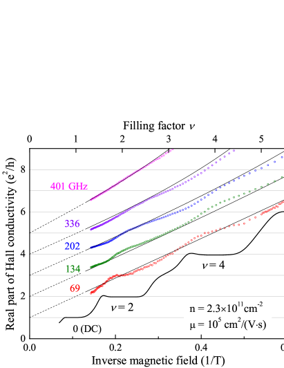
Figure 4: Evolution of the Hall conductivity with increasing frequency for sample #1 (Tab. 1). The DC conductivity, shown by the black solid line, exhibits plateaus near the even filling factors $\nu=nh/eB$. High-frequency curves are shifted by 1 for clarity. At 69 GHz (red) the real part of $\sigma_{xy}$ has a narrow plateau only around $\nu=2$. Further increasing of the frequency leads to the smearing of the plateau and to the suppression of quantum deviations from classical Drude behavior (shown by thin black curves).

In order to trace the evolution of the quantum plateaus with increasing frequency, the real part of the Hall conductivity in sample #1 is plotted as a function of the inverse magnetic field in Fig. 4. The DC conductance, shown by the black curve, demonstrates wide plateaus at even filling factors $\nu=nh/eB$. In a separate experiment, the DC measurement was extended up to 14 T. The plateau at $\nu=1$ was also resolved. The overall behavior of the high-frequency data is well described by the classical Drude theoryPalik and Furdyna (1970), shown by thin black curves. At frequencies below 250 GHz, the cyclotron resonance is located in low magnetic fields, thus the fitting curves in Fig. 4 are close to a straight line $\operatorname{Re}\sigma_{xy}\propto B^{-1}\propto\nu$. At 69 GHz (red symbols) a plateau at $\nu=2$ can be detected in the experimental conductivity. The width of this plateau is 30% of that in the DC data. There is no interval with constant $\operatorname{Re}\sigma_{xy}(B)$ at 134 GHz (green symbols), and even the slope $\partial\sigma_{xy}/\partial\nu$ does not tend to zero at $\nu=2$. At 134 GHz, the filling of the second Landau level is revealed as a slight quantum deviation from the classical curve $\operatorname{Re}\sigma_{\text{Drude}}(B)$. At higher frequencies, the amplitude of the quantum deviation decreases. At 401 GHz (magenta symbols) no signs of the initial plateau can be detected visually on the plot. The position of the quantum feature in $\operatorname{Re}\sigma_{xy}(B)$ can be determined by tracking the minimum slope that shifts to lower magnetic fields with increasing frequency. The plateaus at higher filling factors are smeared out at 69 GHz and they disappear in a similar way.

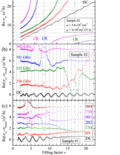
Figure 5: (a) The Hall conductivity for sample #2 (Tab. 1) at different frequencies as a function of the inverse magnetic field and the Landau filling factor $\nu=nh/eB$. The positions of the cyclotron resonance are denoted by “CR”. The solid gray lines are classical Drude fits. (b, c) The difference between the experimental data and the classical fits for samples #2 and #1, respectively. For clarity, the data sets are shifted by $2e^{2}/h$ in (a, b) and by $e^{2}/h$ in (c). All panels are matched by $\nu$ and the magnetic field is indicated for sample #2 (a, b).

In comparison with sample #1, sample #2 had a higher electron mobility and electron density (see Tab. 1). The evolution of the real part of $\sigma_{xy}$ for sample #2 is shown in Fig. 5(a). Similar to sample #1, the cyclotron resonance in high-frequency Hall conductivity can be approximated by classical Drude fits. Quantum oscillations, corresponding to the filling of Landau levels, can be detected in the high-field region as well. The difference between the experimental conductivity and the classical Drude fit is plotted in Fig. 5(b). The large discrepancy at $B\approx B_{c}$ is due to the large value of optical conductivity (approaching 100 e²/h) along with the steep slope $\partial\sigma_{xy}/\partial\nu$. A maximal amplitude of the quantum deviations in the sample #2 is achieved at filling factors of $\nu>10$, while the oscillations attenuate with increasing filling factor $\nu$ in sample #1, see Fig. 5(c).

Although no flat plateaus can be detected in the high-frequency $\sigma_{xy}$, the amplitude of the quantum deviations at 236 GHz (Fig. 5(b)) above $\nu=10$ is comparable with the amplitude of quantum deviations in the DC conductance. The phase of the AC deviations is shifted with respect to the DC data. This effect is better seen in Fig. 5(b) when comparing DC and 236 GHz curves around $\nu=12$. The DC $\sigma_{xy}$ and $\sigma_{\text{Drude}}$ coincide at integer filling factors $\nu=10$, 12, 14, …, and their difference $(\sigma_{xy}-\sigma_{\text{Drude}})$ peaks at half integers above and below (e.g. positive peaks at $\nu=9.5$, 11.5, 13.5, …and negative peaks at 10.5, 12.5, 14.5, …) However for the AC data at 236 GHz the difference has positive peaks at $\nu=10$, 12, 14, etc. A similar phase shift can be observed in sample #1 around $\nu=3$, see Fig. 5(c). The shift of oscillations in the difference $(\sigma_{xy}-\sigma_{\text{Drude}})$ corresponds to a shift of positions of the minimal slope $\operatorname{Re}(\partial\sigma_{xy}/\partial\nu)$ towards higher values of $\nu$ and towards smaller magnetic fields. Similar effect was reported previously Galchenkov et al. (1987); Ikebe et al. (2010) and attributed to the difference in the Landau level broadening and in the localization length between adjacent Landau levels.

According to the relation $\Omega_{c}\propto B\propto 1/\nu_{c}$, the cyclotron resonance shifts to lower $\nu$ as the radiation frequency increases. Figures 5(b, c) demonstrate that the quantum oscillations become attenuated to the right of the CR ($\nu>\nu_{c}$), where the radiation frequency exceeds the cyclotron gap ($\omega>\Omega_{c}$).

IV.2 Imaginary part of $\sigma_{xy}(\omega)$

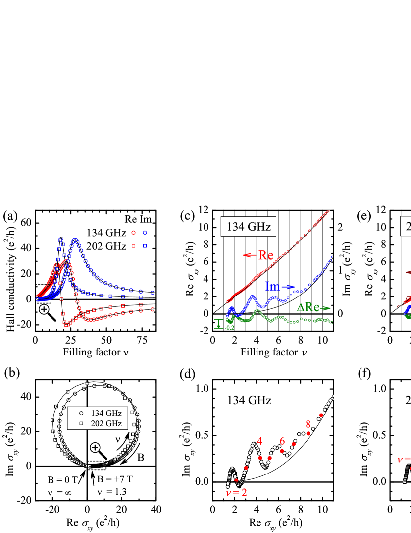
Figure 6: The complex Hall conductivity $\sigma_{xy}$ in sample #1 (Tab. 1) at 134 and 202 GHz. (a) Real and imaginary parts of $\sigma_{xy}$ are shown as a function of the Landau filing factor $\nu=nh/eB$. The overall resonance behavior is well described by the Drude model (black solid lines). Panel (b) shows $\sigma_{xy}$ on a complex plane as a parametric plot with the filling factor as a parameter. In the low-$\nu$ limit (c–f), where QHE is observed in DC, the imaginary part of $\sigma_{xy}$ demonstrates substantial periodic deviations from the classical curve (c, e). These deviations are comparable to the deviations in the real part, shown by green symbols on the same scale. In panels (d, f) the integer values of $\nu$ are indicated by red symbols.

While the Hall conductivity is a real number in the static case, it becomes a complex number with a nonzero imaginary part at finite frequencies. Figures 6(a,c,e) show the experimentally obtained $\sigma_{xy}(\nu)$ (symbols) at 134 and 202 GHz together with the Drude fits (solid curves) for sample #1. Figures 6(b,d,f) show $\sigma_{xy}$ on a complex plane as a parametric plot with the filling factor $\nu$ as a parameter. The sweep of the magnetic field from 7 to 0 T corresponds to the change of $\nu$ from 1.32 to $\infty$. In this representation, classical theory produces a circle-like curve, depicted in Fig. 6(b) by black solid lines. For higher frequencies the curve is getting closer to a perfect circle that is centered on the imaginary axis and passes through the origin of the coordinates. The resonance behavior of experimental conductivity is well described by the classical Drude theory, see Fig. 6(a, b). However, when only a few Landau levels are occupied, $\sigma_{xy}$ demonstrates substantial deviations from the classical curve, see Fig. 6(c–f). Due to experimental limitations, the complex argument of $\sigma_{xy}(\nu)$ was determined up to an unknown constant value, which can be estimated by comparing with the Drude fit. In Fig. 6 this value was chosen to match the theoretical and experimental curves near $\nu=10$, where the quantum deviations are faded out. In this case, the imaginary part of the quantum corrections appears to be positive nearly everywhere and the imaginary part of $\sigma_{xy}$ tends to preserve its original sign. As discussed above, in the real part of $\sigma_{xy}$, the deviations can be regarded as remnants of the DC Hall plateaus. Figures 6(c, e) show the real part of the difference $(\sigma_{xy}-\sigma_{\text{Drude}})$, depicted by green symbols on the same scale as the imaginary part. These plots demonstrate that the quantum oscillations have similar amplitudes in the real and imaginary parts and that the phases are shifted by $\approx\pi/2$. The broken periodicity below $\nu=2$ is likely due to the presence of the quantum plateau at $\nu=1$, which is the only odd plateau resolved in this sample (Fig. 4).

V Discussion

The most striking feature of the QHE at zero frequency is the exact quantization of the Hall resistance $R_{xy}$, which is a macroscopic property of a whole sample, directly obtained in DC experiments. This fact alone does not prove that $\sigma_{xy}$ is also exactly quantized Kuchar et al. (1987), because local inhomogeneities of the two-dimensional gas are always present in a real sample. Unlike the contact techniques, the spectroscopic experiments test $\sigma_{xy}$ directly. Experiments at 30 GHz Kuchar et al. (1987) demonstrated that the plateaus of non-zero width are also present in $\sigma_{xy}$. As shown above, the plateaus in $\sigma_{xy}$ disappear at higher frequencies. For the samples in this study the critical frequency lies near 100 GHz. Above this frequency the two-dimensional electron gas loses its QHE features and the Hall conductivity follows the classical Drude model.

Although the IQHE has been extensively studied theoretically, only a few works have addressed the Hall conductivity in a high-frequency regime Morimoto et al. (2009). When calculating the Hall conductivity in a linear approximation, a common approach is to apply linear perturbation theory (Kubo formalism) to a model system. The theoretical models of IQHE consider non-interacting fermions in a strong magnetic field, placed in a model potential, which simulates the presence of impurities and constraints in a sample. Depending on the chosen potential, the analysis of such models can be conducted analytically or numerically.

In Refs. [Morimoto et al., 2009,Morimoto et al., 2010] the high-frequency Hall conductivity was calculated using a numerical method of exact diagonalization. In order to model the disorder, the authors treated randomly distributed Gaussian scatterers. As calculated within this model, $\sigma_{xy}(\omega)$ was found to retain the Hall plateaus in the THz range. In Ref. [Ikebe et al., 2010], these model results were referred to justify the procedure of averaging $\sigma_{xy}(\omega,\nu)$ over a range of frequencies from 0.5 to 1.2 THz. The resulting averaged $\widetilde{\sigma}_{xy}(\nu)$ had a plateau-like feature of vanishing width in comparison with a wide plateau in DC. This experimental fact, reported in Ref. [Ikebe et al., 2010], indicates that the plateaus actually smeared out below 1.2 THz. The procedure of averaging should be reconsidered, since it only masks the disappearance of the Hall plateaus for increasing frequencies.

In earlier works, the high-frequency Hall conductivity was treated analytically in two opposite limits: for scatterers with $\delta$-potential Lozovik et al. (1984) and for a slowly varying potential of impurities Apenko and Lozovik (1985). In Ref. [Lozovik et al., 1984], the Hall conductivity was obtained within the $\delta$-impurity model Prange (1981) as a function of electron density $n$. At finite frequencies, the dependence $\operatorname{Re}\sigma_{xy}(n)$ is predicted to have a single-dip or a double-dip structure instead of a flat plateau at DC. A monotonic dependence $\operatorname{Re}\sigma_{xy}(n)$ is achieved only if both negative and positive $\delta$-impurities are present in the calculation and the Landau level broadening exceeds the cyclotron energy. The last condition was likely not fulfilled in this study’s samples, while the experimental high-frequency $\operatorname{Re}\sigma_{xy}(B)$ was monotonic in the vicinity of the DC plateaus. Unfortunately, the imaginary part of $\sigma_{xy}$ was not treated in Ref. [Lozovik et al., 1984] and no explicit estimation was given for the critical frequency $f_{0}$ at which the plateaus were destroyed. However, the consideration can be extended. In particular, the critical frequency $f_{0}$ can be shown to be close to the half-width $\Gamma/(4\pi\hbar)$ of the corresponding broadened Landau level Lozovik (2017). If the level broadening is assumed to be caused by the scattering on short-range ionized impurities, then the width can be estimated as Tsuneya and Yasutada (1974):

$$\Gamma=\hbar\sqrt{\frac{2\Omega_{c}}{\pi\tau}}.$$ (2)

Since the cyclotron frequency $\Omega_{c}=eB/m$ increases with magnetic field, the plateaus at small filling factors are expected to be retained at higher radiation frequencies. Using the parameters in Tab. 1 for sample #1, the critical frequency is obtained as $f_{0}=47\sqrt{B}$ GHz. For the plateaus at $\nu=2$ and $\nu=4$, the estimated critical frequencies are 102 and 72 GHz, respectively. In agreement with this estimation, the plateau at $\nu=2$ at 69 GHz was experimentally observed. The plateau at $\nu=4$ was not resolved, as the corresponding critical frequency of 72 GHz is close to the radiation frequency. The plateaus at $\nu>4$ are already absent at $f\geq 69$ GHz, since they occur in $R_{xy}$ at even lower magnetic fields. Due to the longer relaxation time in sample #2 (Tab. 1), the estimated Landau level width was smaller and the critical frequency was lower than in sample #1. For this reason, no plateaus in high-frequency conductivity could be observed in sample #2.

If Eq. (2) is applied to the case of HgTe films Shuvaev et al. (2016) and to graphene Shimano et al. (2013), critical frequencies of 1 THz and $\approx 3$ THz are obtained, respectively. These higher values are formally achieved due to the smaller effective masses and the shorter relaxation times in the CdHgTe wells and in graphene. The direct application of Eq. (2) to the systems with a strongly non-parabolic dispersion is questionable. However, it is possible that the observation of the quantized Faraday rotation in these materials at higher frequencies is indeed connected to the larger width of the Landau levels.

In Ref. [Apenko and Lozovik, 1985] the Hall conductivity was calculated using the drift approximation Iordansky (1982); Kazarinov and Luryi (1982). In the limit of very high frequencies, $\sigma_{xy}(\nu)$ tended to the classical straight line with a small quantum correction:

$$\sigma_{xy}(\nu)=\nu e^{2}/h+\delta\sigma_{xy}(\nu).$$

As calculated within this model, the term $\delta\sigma_{xy}$ has zero imaginary part, while the experimental $\delta\sigma_{xy}$ has both real and imaginary parts of a similar amplitude. The calculation of intermediate frequencies resulted in $\sigma_{xy}$ with a non-zero imaginary part. However, in this case the dependence of $\operatorname{Re}\sigma_{xy}(\nu)$ was not monotonic. Thus, the shape of the smeared quantum plateaus is not described by this approach even qualitatively. The critical frequency calculated in the drift approximation was connected to the level broadening, similar to the case of $\delta$-potential treated above.

None of the existing theoretical models provides a satisfactory description for the shape of the plateaus in the high-frequency Hall conductivity. The numerical method of exact diagonalization predicts the persistence of the plateaus in the THz range. Within this model, a decrease in disorder leads to a decreasing width $\Gamma$ of Landau levels and to a more distinct quantization in $\sigma_{xy}$. In contrast, the analytical methods predict the destruction of the plateaus at frequencies $f>\Gamma/h$. Within these models, a stronger disorder allows the quantum plateaus to occur at higher frequencies. The experimental data presented in this work and in Refs. [Kuchar et al., 1987; Stier et al., 2015; Shimano et al., 2013; Shuvaev et al., 2016] support the result of the analytical methods. An ultimate understanding requires further systematic experimental studies on samples with significantly different electron mobilities and cyclotron masses.

VI Conclusions

The dynamic quantum Hall effect was studied using continuous-wave THz spectroscopy in the frequency range of 69–1100 GHz. A clear frequency dependence of the quantum deviations from the classical Drude model was observed. The extinction of the QHE plateaus took place near 100 GHz. Only small quantum corrections were observed above this frequency. Some theoretical models describe this phenomenon qualitatively, while other models predict the persistence of the plateaus in the high-frequency range. The results of this work will stimulate efforts towards a complete understanding of the IQHE.

VII Acknowledgments

We acknowledge valuable discussion with Yu. Lozovik and Zh. Gevorkyan. This work was supported by Austrian Science Funds (W–1243, P27098–N27, I3456–N27).

References

- Klitzing et al. (1980) K. v. Klitzing, G. Dorda, and M. Pepper, “New method for high-accuracy determination of the fine-structure constant based on quantized Hall resistance,” Phys. Rev. Lett. 45, 494–497 (1980).
- Kuchar et al. (1986) F. Kuchar, R. Meisels, G. Weimann, and W. Schlapp, “Microwave Hall conductivity of the two-dimensional electron gas in GaAs-AlxGa1-xAs,” Phys. Rev. B 33, 2965–2967 (1986).
- Galchenkov et al. (1987) L. A. Galchenkov, I. M. Grodnenskii, M. V. Kostovetskii, and O. R. Matov, “Frequency dependence of the Hall conductivity of a 2D electron gas,” JETP Lett. 46, 542 (1987).
- Hohls et al. (2002) F. Hohls, U. Zeitler, R. J. Haug, R. Meisels, K. Dybko, and F. Kuchar, “Dynamical scaling of the quantum Hall plateau transition,” Phys. Rev. Lett. 89, 276801 (2002).
- Volkov and Mikhailov (1985) V. A. Volkov and S. A. Mikhailov, “Quantization of the Faraday effect in systems with a quantum Hall effect,” JETP Lett. 41, 476 (1985).
- Shimano et al. (2013) R. Shimano, G. Yumoto, J. Y. Yoo, R. Matsunaga, S. Tanabe, H. Hibino, T. Morimoto, and H. Aoki, “Quantum Faraday and Kerr rotations in graphene,” Nat. Commun. 4, 1841 (2013).
- Okada et al. (2016) K. N. Okada, Y. Takahashi, M. Mogi, R. Yoshimi, A. Tsukazaki, K. S. Takahashi, N. Ogawa, M. Kawasaki, and Y. Tokura, “Terahertz spectroscopy on Faraday and Kerr rotations in a quantum anomalous Hall state,” Nat. Commun. 7, 12245 (2016).
- Wu et al. (2016) Liang Wu, M. Salehi, N. Koirala, J. Moon, S. Oh, and N. P. Armitage, “Quantized Faraday and Kerr rotation and axion electrodynamics of the surface states of three-dimensional topological insulators,” Science 354, 1124 (2016).
- Dziom et al. (2017a) V. Dziom, A. Shuvaev, A. Pimenov, G. V. Astakhov, C. Ames, K. Bendias, J. Böttcher, G. Tkachov, E. M. Hankiewicz, C. Brüne, and L. W. Buhmann, H. Molenkamp, “Observation of the universal magnetoelectric effect in a 3D topological insulator,” Nat. Commun. 8, 15197 (2017a).
- Tse (2016) Wang-Kong Tse, “Coherent magneto-optical effects in topological insulators: Excitation near the absorption edge,” Phys. Rev. B 94, 125430 (2016).
- Lee and Tse (2017) W.-R. Lee and W.-K. Tse, “Dynamical quantum anomalous Hall effect in strong optical fields,” Phys. Rev. B 95, 201411 (2017).
- Ikebe et al. (2010) Y. Ikebe, T. Morimoto, R. Masutomi, T. Okamoto, H. Aoki, and R. Shimano, “Optical Hall effect in the integer quantum Hall regime,” Phys. Rev. Lett. 104, 256802 (2010).
- Stier et al. (2015) A. V. Stier, C. T. Ellis, J. Kwon, H. Xing, H. Zhang, D. Eason, G. Strasser, T. Morimoto, H. Aoki, H. Zeng, B. D. McCombe, and J. Cerne, “Terahertz dynamics of a topologically protected state: Quantum Hall effect plateaus near the cyclotron resonance of a two-dimensional electron gas,” Phys. Rev. Lett. 115, 247401 (2015).
- Failla et al. (2016) M. Failla, J. Keller, G. Scalari, C. Maissen, J. Faist, C. Reichl, W. Wegscheider, O. J. Newell, D. R. Leadley, M. Myronov, and J. Lloyd-Hughes, “Terahertz quantum Hall effect for spin-split heavy-hole gases in strained Ge quantum wells,” New J. Phys. 18, 113036 (2016).
- Sebestyen (1982) T. Sebestyen, “Models for ohmic contacts on graded crystalline or amorphous heterojunctions,” Solid-State Electron. 25, 543 (1982).
- Lakhani (1984) A. A. Lakhani, “The role of compound formation and heteroepitaxy in indium-based ohmic contacts to GaAs,” J. Appl. Phys. 56, 1888 (1984).
- Baba et al. (1983) T. Baba, T. Mizutani, and M. Ogawa, “Elimination of persistent photoconductivity and improvement in Si activation coefficient by Al spatial separation from Ga and Si in Al-Ga-As:Si solid system. A novel short period AlAs/n-GaAs superlattice,” Jpn. J. Appl. Phys. 22, L627 (1983).
- Nathan (1986) M. I. Nathan, “Persistent photoconductivity in AlGaAs/GaAs modulation doped layers and field effect transistors: A review,” Solid-State Electron. 29, 167 (1986).
- Berreman (1972) D. W. Berreman, “Optics in stratified and anisotropic media: 4x4-matrix formulation,” J. Opt. Soc. Am. 62, 502 (1972).
- Dziom et al. (2017b) V. Dziom, A. Shuvaev, N. N. Mikhailov, and A. Pimenov, “Terahertz properties of Dirac fermions in films with optical doping,” 2D Mater. 4, 024005 (2017b).
- Shuvaev et al. (2012) A. M. Shuvaev, G. V. Astakhov, C. Brüne, H. Buhmann, L. W. Molenkamp, and A. Pimenov, “Terahertz magneto-optical spectroscopy in thin films,” Semicond. Sci. Technol. 27, 124004 (2012).
- Palik and Furdyna (1970) E. D. Palik and J. K. Furdyna, “Infrared and microwave magnetoplasma effects in semiconductors,” Rep. Prog. Phys. 33, 1193 (1970).
- Kuchar et al. (1987) F. Kuchar, R. Meisels, K. Y. Lim, P. Pichler, G. Weimann, and W. Schlapp, “Hall conductivity at microwave and submillimeter frequencies in the quantum Hall effect regime,” Phys. Scr. 1987, 79 (1987).
- Morimoto et al. (2009) T. Morimoto, Y. Hatsugai, and H. Aoki, “Optical Hall conductivity in ordinary and graphene quantum Hall systems,” Phys. Rev. Lett. 103, 116803 (2009).
- Morimoto et al. (2010) T. Morimoto, Y. Avishai, and H. Aoki, “Dynamical scaling analysis of the optical Hall conductivity in the quantum Hall regime,” Phys. Rev. B 82, 081404 (2010).
- Lozovik et al. (1984) Yu. E. Lozovik, V. M. Farztdinov, and Zh. S. Gevorkyan, “Dynamic quantum Hall effect,” JETP Lett. 39, 179 (1984).
- Apenko and Lozovik (1985) S. M. Apenko and Yu. E. Lozovik, “Quantization of the Hall conductivity of a two-dimensional electron gas in a strong magnetic field,” J. Exp. Theor. Phys. 62, 328 (1985).
- Prange (1981) R. E. Prange, “Quantized Hall resistance and the measurement of the fine-structure constant,” Phys. Rev. B 23, 4802 (1981).
- Lozovik (2017) Yu. E. Lozovik, “private communications,” (2017).
- Tsuneya and Yasutada (1974) A. Tsuneya and U. Yasutada, “Theory of oscillatory g factor in an MOS inversion layer under strong magnetic fields,” J. Phys. Soc. Jpn. 37, 1044 (1974).
- Shuvaev et al. (2016) A. Shuvaev, V. Dziom, Z. D. Kvon, N. N. Mikhailov, and A. Pimenov, “Universal Faraday rotation in wells with critical thickness,” Phys. Rev. Lett. 117, 117401 (2016).
- Iordansky (1982) S.V. Iordansky, “On the conductivity of two dimensional electrons in a strong magnetic field,” Solid State Commun. 43, 1 – 3 (1982).
- Kazarinov and Luryi (1982) R. F. Kazarinov and S. Luryi, “Quantum percolation and quantization of Hall resistance in two-dimensional electron gas,” Phys. Rev. B 25, 7626–7630 (1982).