Spectroscopic and astrometric radial velocities: Hyades as a benchmark

Abstract

We study the accuracy of spectroscopic RVs by comparing spectroscopic and astrometric RVs for stars of the Hyades open cluster. Rather accurate astrometric RVs are available for the Hyades’ stars, based on Hipparcos and on the first Gaia data release. We obtained HARPS spectra for a large sample of Hyades stars, and we homogeneously analysed them. After cleaning the sample from binaries, RV variables, and outliers, 71 stars remained. The distribution of the observed RV difference (spectroscopic – astrometric) is skewed and depends on the star right ascension. This is consistent with the Hyades cluster rotating at $42.3$ m s^-1pc^-1. The two Hyades giants in the sample show, as predicted by gravitational redshift (GR), a spectroscopic RV that is blue-shifted with respect to the dwarfs, and the empirical GR slope is of $626\pm 131$ m $s^{-1}$, in agreement with the theoretical prediction. The difference between spectroscopic and astrometric RVs is very close to zero, within the uncertainties. In particular, the mean difference is of $-33$ m s^-1 and the median is of $-16$ m s^-1 when considering the Gaia-based RVs (corrected for cluster rotation), with a $\sigma$ of $347$ m s^-1, very close to the expected cluster velocity dispersion. We also determine a new value of the cluster centroid spectroscopic RV: $39.36\pm 0.26$ km s^-1. The spectroscopic RV measurements are expected, from simulations, to depend on stellar rotation, but our data do not confirm these predictions. We finally discuss the other phenomena that can influence the RV difference, such as cluster expansion, stellar activity, general relativity, and Galactic potential. Clusters within the reach of current telescopes are expected to show differences of several hundreds m s^-1, depending on their position in the Galaxy.

1 Introduction

The measurement of the Doppler shift between the absorption lines of a star with respect to a reference spectrum is commonly dubbed the stellar “radial velocity” (RV), but in reality these measurements are affected by a number of effects, that are not easy to measure and new definitions of RV have been recently adopted by IAU, one for spectroscopic mesurements, one for astrometric ones (Lindegren & Dravins, 2003, for a full discussion).

Dravins et al. (1999) discuss three methods to obtain astrometric RVs, one of which is suitable for moving groups and clusters. It is based on the concept that the angular extent of a cluster changes with time because, thanks to its RV, its distance will change. Unfortunately, precise astrometric RVs are only available for a small number of stars and for a few open clusters (Madsen et al., 2002, M02 hereafter).

The early comparison between spectroscopic and astrometric RVs for the stars of the Hyades has shown a fair agreement between the two measurements, and a potential dependence of the RV difference on the stellar spectral type and rotational velocity (M02). Amongst the effects affecting the spectroscopic measurements but not the astrometric ones, GR is likely the most prominent, since it affects differentially non-degenerate stars of the same cluster of up to several hundreds m s^-1 and white dwarfs up to km s^-1. On a previous study of giants and dwarfs in the open cluster M67, Pasquini et al. (2011) did not find evidence for GR, when measuring the RVs by using cross correlation techniques and the same digital mask for all the stars. The authors generated synthetic spectral lines with 3D atmospheres models, and found that the increased photospheric blue shift in solar-type main sequence stars roughly compensates the lower GR effect in evolved stars. These first results show a rather intriguing situation, and makes the problem worth to be studied in more detail.

We present a comparison between spectroscopic RV data collected with the HARPS spectrograph (Mayor et al., 2003) and astrometric data from M02. While developing this work, the Gaia Mission provided its first data release (Gaia Collaboration et al., 2017, G17 henceforth) with new astrometric data and a potentially more accurate estimate of the space velocity of the cluster, which is the only information we need to estimate astrometric RVs. Some Gaia data are not available for Hyades stars (mostly bright) because of reduction issues that may be fixed in the future, but they can be replaced by other data (specifically the equatorial coordinates $\alpha$ and $\delta$) for the calculation of astrometric RVs (see Sect. 2.2 for more details).

The main questions we address in this work is to which extent astrometric and spectroscopic RV measurements agree, and to which extent the difference between spectroscopic and astrometric RVs are affected by stellar activity, GR, atmospheric 3D effects, cluster expansion, galactic potential. We note that, since the results of two independent methods (Doppler vs. astrometric) are compared, the accuracy of the measurements matters, rather than their precision. This is a rare case, since, in general, the RV variations with time (and therefore precision) is what most users measure.

Relevant data about the Hyades are presented in Sect. 2, together with our HARPS observations and the estimate of the physical stellar parameters used in our analysis. A first analysis of the HARPS RV measurements is presented in Sec. 3, where they are compared with astrometric and spectroscopic RVs from the literature. A more detailed discussion between HARPS and astrometric RVs is provided in Sect. 4, where major and minor effects that may distort these measurements are discussed and the results of our 3D simulations are applied. The major effects are analysed in more detail in Sect. 5, where an accurate GR measurement is obtained for the Hyades stars. A HARPS-based cluster RV is determined in Sect. 6 by considering the spatial distribution of the Hyades members. Finally, our conclusions are summarized in Sect. 7.

2 Hyades: the benchmark test

The Hyades is a relatively young cluster, with an age of $\sim$ 625 $\pm$ 50 $\rm{Myr}$ (P98), and it is the closest open cluster to the Sun ($\sim$ 46.5 pc, van Leeuwen, 2009). Several astrometric studies of the Hyades exist, based on Hipparcos measurements (P98, M02, de Bruijne 2001, van Leeuwen 2007), and recently G17 provided a first Gaia solution. For this work we use as a baseline the M02 study, that provided a clean sample, astrometric RVs for al stars and compared them with the spectroscopic ones.

The Hyades metallicity has been studied in detail ($[Fe/H]=0.18$ dex, Dutra-Ferreira et al. 2016) and the good parallaxes measurements coupled to the other observations make it possible to compute rather precise stellar parameters. Hyades stars have also been targets of planet searches using RVs (Cochran et al., 2002; Paulson et al., 2004) and one of the four Hyades giants was reported to host a giant planet. More recently, Quinn et al. (2014) reported the discovery of the first hot Jupiter orbiting a K dwarf HD 285507 in this cluster. The relevance of these studies for the present work is mainly that Paulson et al. (2004) constrained the spectroscopic RV jitter of typical solar-type stars in the Hyades to less than 40 m s^-1. This jitter provides therefore a fundamental limit to the accuracy that can be obtained from the measurement of a single spectrum. Even if the HARPS RV precision is of a few m s^-1 or less, the accuracy of the spectroscopic RV will be limited by this jitter, having only one observation/star.

A total of 218 stars, selected from the list of P98, were observed, out of which 131 match with the list of M02, which is cleaned for membership and some binarity.

Table 1: Selected objects in the Hyades cluster.

#	HIP	SpType	$V_{\rm mag}$	$(B-V)$	$RV_{\rm P98}^{\rm Spectr.}$	$RV_{\rm M02}^{\rm Astrom.}$	$RV_{\rm G17}^{\rm Astrom.}$	$RV_{\rm HARPS}$	FWHM	$S/N$	Flag
			(mag)	(mag)	(km s-1)	(km s-1)	(km s-1)	(km s-1)	(km s-1)
1	13600	K0	8.83	0.704 $\pm$ 0.023	30.41 $\pm$ 0.23	27.73 $\pm$ 0.58	27.59 $\pm$ 0.13	31.1452 $\pm$ 0.0004	7.0	116	0
2	16529	G5	8.88	0.844 $\pm$ 0.000	32.72 $\pm$ 0.17	32.47 $\pm$ 0.59	32.34 $\pm$ 0.14	32.0867 $\pm$ 0.0007	7.5	116	0
3	16908	G5	9.35	0.917 $\pm$ 0.001	33.56 $\pm$ 0.21	33.39 $\pm$ 0.59	33.26 $\pm$ 0.14	31.6168 $\pm$ 0.0007	7.4	116	0
4	18327	K2	8.99	0.895 $\pm$ 0.001	36.79 $\pm$ 0.13	36.03 $\pm$ 0.59	35.90 $\pm$ 0.15	36.4212 $\pm$ 0.0010	8.5	97	0
5	19098	K2	9.31	0.890 $\pm$ 0.008	37.61 $\pm$ 0.05	37.16 $\pm$ 0.59	37.03 $\pm$ 0.16	36.8190 $\pm$ 0.0007	8.3	98	0
6	19148	G0	7.85	0.593 $\pm$ 0.005	38.04 $\pm$ 0.17	37.44 $\pm$ 0.59	37.31 $\pm$ 0.16	37.5821 $\pm$ 0.0009	10.7	131	0
7	19365	G0IV	8.27	0.637 $\pm$ 0.002	37.92 $\pm$ 0.15	35.57 $\pm$ 0.59	35.45 $\pm$ 0.15	38.8555 $\pm$ 0.0012	10.0	122	0
8	19781	G5V	8.45	0.693 $\pm$ 0.011	39.24 $\pm$ 0.06	38.43 $\pm$ 0.60	38.30 $\pm$ 0.16	38.1808 $\pm$ 0.0013	9.3	97	0
9	19796	F8V	7.11	0.514 $\pm$ 0.008	38.50 $\pm$ 0.15	38.65 $\pm$ 0.60	38.52 $\pm$ 0.16	38.2816 $\pm$ 0.0042	22.6	130	0
10	20146	G8V	8.47	0.721 $\pm$ 0.016	38.80 $\pm$ 0.08	38.66 $\pm$ 0.60	38.53 $\pm$ 0.16	38.0862 $\pm$ 0.0010	9.3	124	0
11	20205	G8III	3.65	0.981 $\pm$ 0.012	39.28 $\pm$ 0.11	38.91 $\pm$ 0.60	38.79 $\pm$ 0.16	38.5485 $\pm$ 0.0007	8.5	116	0
12	20480	G9V	8.84	0.758 $\pm$ 0.003	39.24 $\pm$ 0.24	38.56 $\pm$ 0.60	38.44 $\pm$ 0.16	38.7314 $\pm$ 0.0009	8.2	105	0
13	20492	K1V	9.11	0.855 $\pm$ 0.018	40.29 $\pm$ 0.06	39.38 $\pm$ 0.60	39.26 $\pm$ 0.16	39.5077 $\pm$ 0.0010	8.4	100	0
14	20557	F8V	7.13	0.518 $\pm$ 0.014	38.94 $\pm$ 0.13	38.59 $\pm$ 0.60	38.47 $\pm$ 0.16	38.2739 $\pm$ 0.0038	17.2	102	0
15	20614	F4V	5.97	0.378 $\pm$ 0.014	36.60 $\pm$ 1.20	39.06 $\pm$ 0.60	38.94 $\pm$ 0.16	31.9955 $\pm$ 0.0074	9.4	175	0
16	20826	F8	7.49	0.560 $\pm$ 0.007	40.22 $\pm$ 0.21	39.99 $\pm$ 0.60	39.86 $\pm$ 0.17	39.6935 $\pm$ 0.0020	13.6	127	0
17	20850	K0V	9.02	0.839 $\pm$ 0.007	40.94 $\pm$ 0.08	39.89 $\pm$ 0.60	39.77 $\pm$ 0.16	40.2936 $\pm$ 0.0009	8.0	98	0
18	20889	K0III	3.53	1.014 $\pm$ 0.006	39.37 $\pm$ 0.06	39.39 $\pm$ 0.60	39.27 $\pm$ 0.16	38.4354 $\pm$ 0.0004	9.0	199	0
19	20949	G5	9.19	0.766 $\pm$ 0.002	39.02 $\pm$ 0.17	38.12 $\pm$ 0.59	38.01 $\pm$ 0.15	38.6972 $\pm$ 0.0011	7.5	76	0
20	20978	K1V	9.08	0.865 $\pm$ 0.013	40.97 $\pm$ 0.06	39.83 $\pm$ 0.60	39.71 $\pm$ 0.16	40.2908 $\pm$ 0.0017	8.6	59	0
21	21099	G8V	8.59	0.734 $\pm$ 0.014	40.62 $\pm$ 0.08	39.51 $\pm$ 0.60	39.39 $\pm$ 0.16	39.8309 $\pm$ 0.0009	8.4	109	0
22	21741	K0V	9.40	0.811 $\pm$ 0.000	41.34 $\pm$ 0.16	39.75 $\pm$ 0.60	39.64 $\pm$ 0.16	40.2362 $\pm$ 0.0013	8.9	84	0
23	22380	F5	8.98	0.833 $\pm$ 0.003	41.62 $\pm$ 0.15	41.27 $\pm$ 0.60	41.16 $\pm$ 0.17	41.7660 $\pm$ 0.0010	8.4	95	0
24	22422	F8	7.72	0.578 $\pm$ 0.009	42.04 $\pm$ 0.14	41.65 $\pm$ 0.60	41.53 $\pm$ 0.17	41.5230 $\pm$ 0.0015	9.6	96	0
25	22566	F8	7.90	0.527 $\pm$ 0.008	42.92 $\pm$ 0.19	41.85 $\pm$ 0.60	41.73 $\pm$ 0.17	42.4678 $\pm$ 0.0025	15.2	126	0
26	23069	G5	8.89	0.737 $\pm$ 0.001	43.68 $\pm$ 0.16	42.48 $\pm$ 0.60	42.37 $\pm$ 0.17	42.9643 $\pm$ 0.0009	7.6	100	0
27	23498	K0	9.00	0.765 $\pm$ 0.002	43.51 $\pm$ 0.19	42.90 $\pm$ 0.60	42.79 $\pm$ 0.17	43.2023 $\pm$ 0.0012	8.9	93	0
28	23750	K0	8.82	0.730 $\pm$ 0.015	42.31 $\pm$ 0.18	42.67 $\pm$ 0.60	42.56 $\pm$ 0.17	42.8852 $\pm$ 0.0012	9.4	101	0
29	24923	K0	9.03	0.765 $\pm$ 0.029	43.70 $\pm$ 0.23	44.17 $\pm$ 0.60	44.07 $\pm$ 0.17	44.5765 $\pm$ 0.0011	9.1	107	0
30	10672	G0	8.55	0.567 $\pm$ 0.021	26.40 $\pm$ 0.32	21.30 $\pm$ 0.56	21.15 $\pm$ 0.12	27.0446 $\pm$ 0.0009	11.0	108	1
31	15300	M0	11.11	1.408 $\pm$ 0.007	29.84 $\pm$ 0.29	30.06 $\pm$ 0.58	29.93 $\pm$ 0.13	29.3413 $\pm$ 0.0031	7.5	45	1
32	15563	K7V:	9.65	1.130 $\pm$ 0.015	30.45 $\pm$ 0.26	31.72 $\pm$ 0.58	31.58 $\pm$ 0.15	31.0463 $\pm$ 0.0006	8.2	99	1
33	15720	–	11.03	1.431 $\pm$ 0.004	28.90 $\pm$ 0.45	30.60 $\pm$ 0.58	30.47 $\pm$ 0.13	29.9547 $\pm$ 0.0023	7.2	59	1
34	16548	M0V:	11.88	1.378 $\pm$ 0.015	26.60 $\pm$ 0.34	33.41 $\pm$ 0.58	33.27 $\pm$ 0.15	28.6738 $\pm$ 0.0029	7.3	45	1
35	17766	M1	10.85	1.340 $\pm$ 0.015	35.40 $\pm$ 0.25	35.51 $\pm$ 0.59	35.37 $\pm$ 0.16	34.9527 $\pm$ 0.0022	7.4	53	1
36	18018	K7	10.17	1.160 $\pm$ 0.040	35.30 $\pm$ 0.12	34.67 $\pm$ 0.59	34.55 $\pm$ 0.15	34.5523 $\pm$ 0.0010	7.6	85	1
37	18322	M0	10.12	1.070 $\pm$ 0.015	37.18 $\pm$ 0.22	36.32 $\pm$ 0.59	36.18 $\pm$ 0.16	36.2453 $\pm$ 0.0008	8.1	89	1
38	18946	K5	10.12	1.095 $\pm$ 0.119	36.93 $\pm$ 0.26	36.76 $\pm$ 0.59	36.63 $\pm$ 0.15	36.0967 $\pm$ 0.0008	7.8	107	1
39	19082	–	11.41	1.347 $\pm$ 0.005	38.33 $\pm$ 0.22	36.96 $\pm$ 0.59	36.83 $\pm$ 0.15	37.4701 $\pm$ 0.0028	7.6	46	1
40	19207	K5	10.49	1.180 $\pm$ 0.015	38.95 $\pm$ 0.23	37.56 $\pm$ 0.59	37.43 $\pm$ 0.16	38.1161 $\pm$ 0.0016	8.1	64	1
41	19263	K0	9.94	1.005 $\pm$ 0.012	38.72 $\pm$ 0.05	37.53 $\pm$ 0.59	37.41 $\pm$ 0.16	38.0033 $\pm$ 0.0008	7.8	105	1
42	19316	–	11.28	1.327 $\pm$ 0.004	38.43 $\pm$ 0.28	37.91 $\pm$ 0.59	37.78 $\pm$ 0.16	37.9994 $\pm$ 0.0029	7.7	44	1
43	19441	K5V	10.10	1.192 $\pm$ 0.011	39.24 $\pm$ 0.16	38.15 $\pm$ 0.59	38.01 $\pm$ 0.16	38.2760 $\pm$ 0.0009	7.7	98	1
44	19808	K5	10.69	1.204 $\pm$ 0.008	40.51 $\pm$ 0.15	38.58 $\pm$ 0.60	38.45 $\pm$ 0.16	39.0411 $\pm$ 0.0020	7.7	52	1
45	19834	K2	11.56	1.363 $\pm$ 0.010	38.79 $\pm$ 0.36	38.53 $\pm$ 0.60	38.40 $\pm$ 0.16	38.2546 $\pm$ 0.0026	7.7	51	1
46	19862	M2	10.96	0.924 $\pm$ 0.301	38.96 $\pm$ 0.17	38.46 $\pm$ 0.60	38.34 $\pm$ 0.16	38.6097 $\pm$ 0.0017	7.2	58	1
47	20357	F5V	6.60	0.412 $\pm$ 0.014	39.20 $\pm$ 0.21	39.20 $\pm$ 0.60	39.07 $\pm$ 0.16	39.1183 $\pm$ 0.0075	28.5	119	1
48	20527	K5.5Ve	10.89	1.288 $\pm$ 0.002	40.64 $\pm$ 0.26	39.46 $\pm$ 0.60	39.34 $\pm$ 0.16	39.7234 $\pm$ 0.0019	7.4	55	1
49	20605	M0.5Ve	11.66	1.408 $\pm$ 0.013	40.20 $\pm$ 0.36	39.40 $\pm$ 0.60	39.28 $\pm$ 0.16	39.9854 $\pm$ 0.0060	9.4	38	1
50	20745	M0V	10.50	1.358 $\pm$ 0.002	41.38 $\pm$ 0.18	39.84 $\pm$ 0.60	39.71 $\pm$ 0.16	40.2956 $\pm$ 0.0022	7.6	56	1
51	20762	K7	10.48	1.146 $\pm$ 0.001	41.22 $\pm$ 0.21	39.83 $\pm$ 0.60	39.70 $\pm$ 0.16	40.2113 $\pm$ 0.0018	8.2	57	1
52	20827	K0	9.48	0.929 $\pm$ 0.005	40.46 $\pm$ 0.07	39.82 $\pm$ 0.60	39.70 $\pm$ 0.16	39.7185 $\pm$ 0.0008	8.0	103	1
53	21138	K5Ve	11.02	1.280 $\pm$ 0.014	41.28 $\pm$ 0.21	40.13 $\pm$ 0.60	40.01 $\pm$ 0.16	40.3908 $\pm$ 0.0025	7.7	46	1
54	21256	K8	10.69	1.237 $\pm$ 0.005	41.39 $\pm$ 0.20	39.56 $\pm$ 0.60	39.45 $\pm$ 0.16	40.0236 $\pm$ 0.0013	7.6	74	1
55	21261	–	10.74	1.197 $\pm$ 0.004	41.43 $\pm$ 0.15	39.89 $\pm$ 0.60	39.77 $\pm$ 0.16	40.1629 $\pm$ 0.0015	8.1	69	1

Notes. Columns are HIP: Hipparcos number; SpType: spectral type from the Hipparcos catalogue; $V_{\rm mag}$: visual magnitude; $(B-V)$: colour index; $RV_{\rm P98}^{\rm Spectr.}$: spectroscopic RV from P98; $RV_{\rm M02}^{\rm Astrom.}$: astrometric RV from M02; $RV_{\rm G17}^{\rm Astrom.}$: astrometric RV computed in this work from G17 data; $RV_{\rm HARPS}$: our HARPS RV measurements without zero point correction, from which we subtracted the HARPS mask zero point of $102$ m s^-1 for our analysis (see text); FWHM: full width at half maximum of the HARPS CCF; $S/N$: singal-to-noise ratio at 490 $\mu$m; Flag: quality flag. Flags are 0 and 1 for acceptable HARPS data with higher- and lower-quality CCF shape, respectively; “BY” for BY Dra variables with acceptable CCF shape; “SB” for spectroscopic binaries; and “x” for excluded targets (because of bad-quality CCF).

Table 1: Continued.

#	HIP	SpType	$V_{\rm mag}$	$(B-V)$	$RV_{\rm P98}^{\rm Spectr.}$	$RV_{\rm M02}^{\rm Astrom.}$	$RV_{\rm G17}^{\rm Astrom.}$	$RV_{\rm HARPS}$	FWHM	$S/N$	Flag
			(mag)	(mag)	(km s-1)	(km s-1)	(km s-1)	(km s-1)	(km s-1)
56	21723	K5	10.04	1.073 $\pm$ 0.005	42.50 $\pm$ 0.19	41.08 $\pm$ 0.60	40.96 $\pm$ 0.17	41.6793 $\pm$ 0.0010	7.9	89	1
57	22177	–	10.92	1.277 $\pm$ 0.005	43.16 $\pm$ 0.25	41.71 $\pm$ 0.60	41.59 $\pm$ 0.17	41.9002 $\pm$ 0.0021	7.5	50	1
58	22253	K2III	10.69	1.112 $\pm$ 0.004	41.78 $\pm$ 0.23	40.40 $\pm$ 0.60	40.29 $\pm$ 0.16	40.6158 $\pm$ 0.0014	8.3	71	1
59	22271	K7III	10.61	1.174 $\pm$ 0.005	40.30 $\pm$ 0.17	39.76 $\pm$ 0.60	39.65 $\pm$ 0.16	39.5603 $\pm$ 0.0013	7.2	70	1
60	22654	K0	10.29	1.070 $\pm$ 0.015	42.88 $\pm$ 0.25	41.48 $\pm$ 0.60	41.37 $\pm$ 0.17	41.6956 $\pm$ 0.0012	8.2	76	1
61	23312	K2	9.71	0.957 $\pm$ 0.047	42.21 $\pm$ 0.40	42.94 $\pm$ 0.60	42.82 $\pm$ 0.17	43.0503 $\pm$ 0.0007	7.6	110	1
62	13806	G5	8.92	0.855 $\pm$ 0.008	26.62 $\pm$ 0.21	26.86 $\pm$ 0.57	26.74 $\pm$ 0.12	26.3762 $\pm$ 0.0010	8.6	99	BY
63	13976	G5	7.97	0.926 $\pm$ 0.015	28.35 $\pm$ 0.18	28.60 $\pm$ 0.57	28.46 $\pm$ 0.14	28.9233 $\pm$ 0.0003	7.8	119	BY
64	19786	G0	8.05	0.640 $\pm$ 0.001	39.32 $\pm$ 0.14	38.57 $\pm$ 0.60	38.44 $\pm$ 0.16	38.4077 $\pm$ 0.0011	9.7	122	BY
65	19793	G3V	8.05	0.657 $\pm$ 0.007	38.21 $\pm$ 0.23	37.31 $\pm$ 0.59	37.19 $\pm$ 0.15	37.6314 $\pm$ 0.0011	10.0	138	BY
66	19934	K0V	9.14	0.813 $\pm$ 0.002	38.46 $\pm$ 0.19	37.80 $\pm$ 0.59	37.68 $\pm$ 0.16	38.2191 $\pm$ 0.0006	7.5	136	BY
67	20082	K3V	9.57	0.980 $\pm$ 0.005	39.64 $\pm$ 0.08	38.72 $\pm$ 0.60	38.59 $\pm$ 0.16	38.9685 $\pm$ 0.0008	7.4	98	BY
68	20130	G9V	8.62	0.745 $\pm$ 0.005	39.58 $\pm$ 0.06	38.34 $\pm$ 0.60	38.22 $\pm$ 0.16	38.7177 $\pm$ 0.0006	8.2	160	BY
69	20237	G0V	7.46	0.560 $\pm$ 0.014	38.81 $\pm$ 0.18	38.56 $\pm$ 0.60	38.44 $\pm$ 0.16	38.3962 $\pm$ 0.0018	15.4	168	BY
70	20485	K5V	10.47	1.231 $\pm$ 0.009	39.30 $\pm$ 0.21	39.27 $\pm$ 0.60	39.15 $\pm$ 0.16	38.4992 $\pm$ 0.0019	8.1	59	BY
71	20563	K4V	9.99	1.050 $\pm$ 0.011	39.95 $\pm$ 0.16	39.12 $\pm$ 0.60	39.00 $\pm$ 0.16	39.4498 $\pm$ 0.0008	7.8	111	BY
72	20577	G2V	7.79	0.599 $\pm$ 0.015	38.80 $\pm$ 0.08	39.27 $\pm$ 0.60	39.15 $\pm$ 0.16	37.7569 $\pm$ 0.0013	10.8	136	BY
73	20741	G8V	8.10	0.664 $\pm$ 0.008	40.23 $\pm$ 0.28	39.50 $\pm$ 0.60	39.38 $\pm$ 0.16	38.3392 $\pm$ 0.0011	8.0	89	BY
74	20815	F8V	7.41	0.537 $\pm$ 0.015	39.32 $\pm$ 0.24	39.71 $\pm$ 0.60	39.58 $\pm$ 0.16	39.3271 $\pm$ 0.0026	14.3	108	BY
75	20899	G2V	7.83	0.609 $\pm$ 0.010	39.99 $\pm$ 0.16	39.65 $\pm$ 0.60	39.53 $\pm$ 0.16	39.2047 $\pm$ 0.0013	11.2	137	BY
76	20951	K0V	8.95	0.831 $\pm$ 0.003	40.70 $\pm$ 0.06	39.65 $\pm$ 0.60	39.53 $\pm$ 0.16	39.9421 $\pm$ 0.0010	7.6	82	BY
77	21317	G1V	7.90	0.631 $\pm$ 0.014	40.78 $\pm$ 0.16	40.38 $\pm$ 0.60	40.26 $\pm$ 0.16	40.4391 $\pm$ 0.0012	9.9	120	BY
78	19554	F4V	5.71	0.360 $\pm$ 0.012	36.60 $\pm$ 1.20	38.28 $\pm$ 0.59	38.14 $\pm$ 0.16	36.9090 $\pm$ 0.0045	21.8	152	SB
79	19870	G4V	7.83	0.705 $\pm$ 0.003	38.46 $\pm$ 0.12	37.88 $\pm$ 0.59	37.75 $\pm$ 0.16	20.1114 $\pm$ 0.0015	8.2	123	SB
80	20019	G8V	8.32	0.756 $\pm$ 0.004	38.18 $\pm$ 0.13	38.56 $\pm$ 0.60	38.44 $\pm$ 0.16	-16.0670 $\pm$ 0.0013	12.8	170	SB
81	20419	K8	9.79	1.183 $\pm$ 0.005	40.77 $\pm$ 0.20	39.46 $\pm$ 0.60	39.34 $\pm$ 0.16	33.7640 $\pm$ 0.0014	6.2	101	SB
82	20455	G8III	3.77	0.983 $\pm$ 0.010	39.65 $\pm$ 0.08	39.04 $\pm$ 0.60	38.92 $\pm$ 0.16	37.5875 $\pm$ 0.0004	8.9	213	SB
83	20661	F7V	6.44	0.509 $\pm$ 0.005	39.10 $\pm$ 0.50	39.48 $\pm$ 0.60	39.35 $\pm$ 0.16	41.7982 $\pm$ 0.0035	25.7	184	SB
84	20679	K2V	8.99	0.935 $\pm$ 0.005	37.00 $\pm$ 7.50	39.27 $\pm$ 0.60	39.15 $\pm$ 0.16	40.9931 $\pm$ 0.0011	10.3	119	SB
85	20686	G5V	8.07	0.680 $\pm$ 0.600	40.72 $\pm$ 0.47	39.17 $\pm$ 0.60	39.05 $\pm$ 0.16	37.8761 $\pm$ 0.0014	13.3	149	SB
86	20712	F8V	7.36	0.557 $\pm$ 0.013	38.77 $\pm$ 0.14	38.83 $\pm$ 0.60	38.71 $\pm$ 0.16	24.7244 $\pm$ 0.0013	8.5	97	SB
87	20751	K5	9.45	1.033 $\pm$ 0.005	41.12 $\pm$ 0.20	39.93 $\pm$ 0.60	39.80 $\pm$ 0.17	45.8963 $\pm$ 0.0008	7.7	131	SB
88	20890	G8V	8.62	0.741 $\pm$ 0.014	39.91 $\pm$ 0.08	39.32 $\pm$ 0.60	39.20 $\pm$ 0.16	36.3041 $\pm$ 0.0007	7.8	96	SB
89	21112	F9V	7.78	0.540 $\pm$ 0.019	40.98 $\pm$ 0.31	40.22 $\pm$ 0.60	40.10 $\pm$ 0.17	40.7134 $\pm$ 0.0012	8.4	105	SB
90	21543	G1V	7.53	0.597 $\pm$ 0.012	42.00 $\pm$ 0.33	40.69 $\pm$ 0.60	40.57 $\pm$ 0.17	36.5396 $\pm$ 0.0018	11.6	112	SB
91	22203	G5	8.30	0.665 $\pm$ 0.006	42.42 $\pm$ 0.71	41.44 $\pm$ 0.60	41.32 $\pm$ 0.17	41.3213 $\pm$ 0.0011	8.6	108	SB
92	22224	K0	9.60	0.967 $\pm$ 0.005	40.32 $\pm$ 0.09	41.21 $\pm$ 0.60	41.09 $\pm$ 0.17	42.9301 $\pm$ 0.0015	7.6	58	SB
93	22524	F8	7.29	0.536 $\pm$ 0.011	42.74 $\pm$ 0.17	41.72 $\pm$ 0.60	41.60 $\pm$ 0.17	35.2684 $\pm$ 0.0046	23.0	129	SB
94	23983	A2m	5.43	0.249 $\pm$ 0.010	44.16 $\pm$ 0.14	43.56 $\pm$ 0.60	43.45 $\pm$ 0.17	43.9119 $\pm$ 0.0036	17.2	113	SB
95	13834	F5IV	5.80	0.415 $\pm$ 0.009	28.10 $\pm$ 1.20	27.97 $\pm$ 0.58	27.83 $\pm$ 0.13	27.3858 $\pm$ 0.0066	35.6	136	x
96	18170	F4V	5.97	0.354 $\pm$ 0.017	35.00 $\pm$ 2.50	35.77 $\pm$ 0.59	35.63 $\pm$ 0.15	33.2054 $\pm$ 0.0394	82.8	119	x
97	18658	F5V	6.35	0.417 $\pm$ 0.012	39.10 $\pm$ 1.10	36.94 $\pm$ 0.59	36.81 $\pm$ 0.16	37.7031 $\pm$ 0.0231	79.8	133	x
98	18735	F4V…	5.89	0.319 $\pm$ 0.005	31.70 $\pm$ 1.10	36.58 $\pm$ 0.59	36.45 $\pm$ 0.15	-13.1284 $\pm$ 0.0593	461.8	145	x
99	19261	F3V	6.02	0.397 $\pm$ 0.004	36.35 $\pm$ 0.26	37.65 $\pm$ 0.59	37.52 $\pm$ 0.16	36.3151 $\pm$ 0.0112	40.0	132	x
100	19504	F6V	6.61	0.427 $\pm$ 0.009	37.10 $\pm$ 0.30	37.66 $\pm$ 0.59	37.54 $\pm$ 0.16	37.1204 $\pm$ 0.0085	36.1	150	x
101	19591	K0	9.38	1.090 $\pm$ 0.015	36.90 $\pm$ 0.26	37.03 $\pm$ 0.59	36.91 $\pm$ 0.15	37.0939 $\pm$ 0.0099	6.7	109	x
102	19789	F5V	7.05	0.424 $\pm$ 0.006	38.40 $\pm$ 1.20	37.50 $\pm$ 0.59	37.38 $\pm$ 0.15	29.9866 $\pm$ 0.0388	104.8	143	x
103	19877	F5Vvar	6.31	0.400 $\pm$ 0.015	36.40 $\pm$ 1.20	38.51 $\pm$ 0.60	38.39 $\pm$ 0.16	37.4085 $\pm$ 0.0309	81.2	134	x
104	20215	F7V+…	6.85	0.509 $\pm$ 0.015	39.21 $\pm$ 0.27	38.84 $\pm$ 0.60	38.72 $\pm$ 0.16	38.6342 $\pm$ 0.0028	19.4	151	x
105	20219	F3V…	5.58	0.283 $\pm$ 0.008	42.00 $\pm$ 2.50	39.06 $\pm$ 0.60	38.93 $\pm$ 0.16	3.9646 $\pm$ 0.0298	154.9	162	x
106	20349	F5V	6.79	0.434 $\pm$ 0.015	37.10 $\pm$ 1.20	38.43 $\pm$ 0.60	38.31 $\pm$ 0.16	36.3019 $\pm$ 0.0257	106.1	179	x
107	20350	F6V	6.80	0.441 $\pm$ 0.014	40.80 $\pm$ 2.40	38.80 $\pm$ 0.60	38.68 $\pm$ 0.16	37.8929 $\pm$ 0.0230	59.8	100	x
108	20400	A3m	5.72	0.315 $\pm$ 0.008	37.80 $\pm$ 2.30	39.27 $\pm$ 0.60	39.15 $\pm$ 0.16	65.7194 $\pm$ 0.0090	42.7	166	x
109	20491	F5	7.18	0.462 $\pm$ 0.009	35.90 $\pm$ 0.50	38.04 $\pm$ 0.59	37.92 $\pm$ 0.15	37.4953 $\pm$ 0.0183	52.9	108	x
110	20542	A7V	4.80	0.154 $\pm$ 0.007	39.20 $\pm$ 1.20	39.17 $\pm$ 0.60	39.05 $\pm$ 0.16	37.8405 $\pm$ 0.0191	60.1	192	x
111	20567	F6V	6.96	0.450 $\pm$ 0.018	40.10 $\pm$ 0.60	39.24 $\pm$ 0.60	39.11 $\pm$ 0.16	38.6270 $\pm$ 0.0153	48.0	111	x
112	20842	Am	5.72	0.270 $\pm$ 0.015	37.50 $\pm$ 3.30	38.97 $\pm$ 0.60	38.85 $\pm$ 0.16	35.0437 $\pm$ 0.0275	119.7	185	x
113	20873	F0IV	5.90	0.325 $\pm$ 0.013	40.60 $\pm$ 0.30	39.86 $\pm$ 0.60	39.73 $\pm$ 0.16	36.6681 $\pm$ 0.0275	108.7	110	x
114	20901	A7V	5.02	0.215 $\pm$ 0.003	39.90 $\pm$ 4.10	40.02 $\pm$ 0.60	39.90 $\pm$ 0.17	33.7276 $\pm$ 0.0324	121.3	126	x
115	20948	F6V	6.90	0.451 $\pm$ 0.002	38.62 $\pm$ 0.24	39.65 $\pm$ 0.60	39.53 $\pm$ 0.16	38.9562 $\pm$ 0.0102	42.3	144	x
116	21008	F6V	7.09	0.470 $\pm$ 0.015	38.00 $\pm$ 2.50	39.46 $\pm$ 0.60	39.34 $\pm$ 0.16	39.1536 $\pm$ 0.0130	35.9	90	x
117	21029	A6IV	4.78	0.170 $\pm$ 0.001	41.00 $\pm$ 1.80	39.93 $\pm$ 0.60	39.81 $\pm$ 0.16	32.8012 $\pm$ 0.0430	88.0	144	x
118	21039	Am	5.47	0.258 $\pm$ 0.003	39.56 $\pm$ 0.23	39.99 $\pm$ 0.60	39.87 $\pm$ 0.16	39.1903 $\pm$ 0.0110	36.5	126	x

Table 1: Continued.

#	HIP	SpType	$V_{\rm mag}$	$(B-V)$	$RV_{\rm P98}^{\rm Spectr.}$	$RV_{\rm M02}^{\rm Astrom.}$	$RV_{\rm G17}^{\rm Astrom.}$	$RV_{\rm HARPS}$	FWHM	$S/N$	Flag
			(mag)	(mag)	(km s-1)	(km s-1)	(km s-1)	(km s-1)	(km s-1)
119	21066	F5	7.03	0.472 $\pm$ 0.013	41.35 $\pm$ 0.26	40.34 $\pm$ 0.60	40.22 $\pm$ 0.17	40.3800 $\pm$ 0.0118	40.2	115	x
120	21137	F4V…	6.01	0.338 $\pm$ 0.012	36.00 $\pm$ 2.50	40.09 $\pm$ 0.60	39.97 $\pm$ 0.16	13.7373 $\pm$ 0.0422	184.9	145	x
121	21152	F5V	6.37	0.420 $\pm$ 0.014	39.80 $\pm$ 1.00	40.46 $\pm$ 0.60	40.34 $\pm$ 0.17	39.5813 $\pm$ 0.0216	64.0	113	x
122	21267	F5V	6.62	0.429 $\pm$ 0.012	36.90 $\pm$ 0.90	40.49 $\pm$ 0.60	40.37 $\pm$ 0.17	39.5488 $\pm$ 0.0226	66.1	111	x
123	21459	F5IV	6.01	0.380 $\pm$ 0.600	43.30 $\pm$ 1.20	39.43 $\pm$ 0.60	39.32 $\pm$ 0.16	40.5994 $\pm$ 0.0392	107.3	136	x
124	21474	F5V	6.64	0.442 $\pm$ 0.018	33.70 $\pm$ 1.20	40.54 $\pm$ 0.60	40.42 $\pm$ 0.16	41.1699 $\pm$ 0.0199	65.6	120	x
125	21589	A6V	4.27	0.122 $\pm$ 0.005	44.70 $\pm$ 5.00	40.94 $\pm$ 0.60	40.82 $\pm$ 0.17	39.4782 $\pm$ 0.0547	112.9	168	x
126	21670	A5m	5.38	0.257 $\pm$ 0.009	36.30 $\pm$ 1.20	41.17 $\pm$ 0.60	41.05 $\pm$ 0.17	39.3510 $\pm$ 0.0326	77.4	114	x
127	22550	F6V	6.79	0.543 $\pm$ 0.013	42.44 $\pm$ 0.17	42.15 $\pm$ 0.60	42.03 $\pm$ 0.17	41.5021 $\pm$ 0.0016	10.7	123	x
128	22850	F3IV	6.36	0.292 $\pm$ 0.012	38.40 $\pm$ 2.00	41.61 $\pm$ 0.60	41.50 $\pm$ 0.17	24.9762 $\pm$ 0.0452	174.3	104	x
129	23214	F5V	6.75	0.450 $\pm$ 0.015	42.50 $\pm$ 1.50	42.44 $\pm$ 0.60	42.33 $\pm$ 0.17	42.2957 $\pm$ 0.0132	44.5	120	x
130	26382	F0V	5.53	0.237 $\pm$ 0.011	41.10 $\pm$ 1.20	44.49 $\pm$ 0.60	44.40 $\pm$ 0.17	28.8363 $\pm$ 0.0629	142.5	88	x
131	28356	F5IV	7.78	0.461 $\pm$ 0.015	45.00 $\pm$ 2.50	45.83 $\pm$ 0.59	45.74 $\pm$ 0.18	60.0714 $\pm$ 0.0212	63.1	142	x

2.1 Spectroscopic observations and data reduction

All spectra were acquired with the HARPS (High Accuracy Radial velocity Planet Searcher, Mayor et al., 2003) high-resolution spectrograph (R = 115 000), fed by the 3.6 m telescope in La Silla, Chile. The spectral range covers from 3800 to 6900 Å, with a small gap between 5300–5330 Å because of the arrangement of the CCD mosaic. All the spectra were reprocessed by the last version of the HARPS pipeline (Data Reduction Software version 3.5). All stars have been observed once, in some case observations have been repeated, if the first spectrum casted doubts on the quality of the data. The S/N ratio was always exceeding 50, that implies a photon noise precision of 2 m s^-1 or better for a slow rotating G star; as explained above, photon noise is not limiting the accuracy of the measurements. The list of the observed stars and the measured RV is given in Table 1.

All the spectra were cross correlated with the same digital G2 mask, based on the observed solar spectrum and optimised for the HARPS spectrograph. Being the mask based on an observed solar spectrum, we do not expect a large zero point correction, in fact the G2 HARPS mask has been recently calibrated by Lanza et al. (2016) using solar system bodies, who found a zero point shift of $\sim$100 m s^-1. We will come back on this point in Sect. 3.1.

All the cross-correlation functions (CCFs) and their fits have been checked visually, and a number of stars show lower quality CCFs, either because they present a slope in the CCF continuum, or because multiple peaks are observed, or because the CCF has a non gaussian shape. This is not too surprising, when considering that the original astrometric sample included binaries, as well as stars spanning a large range of spectral types. Hot stars have many fewer lines than the G2 mask and often much broadened by high stellar rotation. Cool stars have many more lines, and therefore present a richer and more complex spectrum. Nevertheless we consider the use of the same, well calibrated mask for all stars an enormous advantage to perform our investigation.

2.2 Astrometric radial velocities

Astrometric RVs for our initial sample were taken from M02, choosing the “Hipparcos” solution, that is the one recommended by the authors. M02 computed the RVs from their Eqs. (1)–(3). The critical input to these equations is the space velocity of the cluster, which is then combined with the right ascension $\alpha$ and declination $\delta$ of the cluster members. These parameters are enough to estimate astrometric RVs from a simple geometrical model assuming that all the cluster members are moving with the same space velocity of the cluster, with no acceleration. Possible accelerations originated, for example, from cluster rotation or expansion are not considered and may introduce biases (see Sect. 3.3). The expected error in the astrometric RV from M02 for each star is of the order of 600 m s^-1. Since the astrometric radial velocity is the the space motion of the cluster projected onto the line of sight for each star, the astrometric radial velocity error is dominated by the error in the cluster velocity vector, and is highly correlated from star to star.

As far as Gaia, G17 provide a more refined space velocity of the cluster in the 3$\times$2 matrix given by their Eq. (4). The first column of the matrix provides the space velocities computed from astrometric information only. The second column uses astrometric and spectroscopic data, so the resulting velocity is affected by the phenomena influencing the spectroscopic RVs discussed in this work. We therefore computed our Gaia based astrometric RVs from the pure astrometric solution of the space velocity: $V_{x}=-6.03\pm 0.08$ km s^-1, $V_{y}=45.56\pm 0.18$ km s^-1, and $V_{z}=5.57\pm 0.06$ km s^-1. The Gaia astrometric RVs are then calculated by simply using Eq. (2) of M02, which is given by:

$$RV_{\rm G17}^{\rm Astrom.}=V_{x}\cos\delta\cos\alpha+V_{y}\cos\delta\sin\alpha+V_{z}\sin\delta.$$ (1)

No parallax is needed and the errors induced by the uncertainty in the ($\alpha$, $\delta$) coordinates is negligible. The typical error associated to the astrometric RVs (G17 RVs hereafter) is around 160 m s^-1, almost one-forth of the M02 errors. Additional astrometric data are provided in Appendix B.

2.3 Mass to radius ratio

Since gravitational redshift depends on the stellar mass to radius ratio, $M/R$, this ratio was computed from the $(B-V)$ color by using theoretical isochrones, obtained from the CMD Web Interface (e.g., Bressan et al., 2012; Tang et al., 2014; Chen et al., 2014, 2015). The used isochrone has log(age/yr) = 8.8 with initial hydrogen and helium compositions (based on the XYZ Calculator web interface with the Grevesse & Sauval 1998 values) $Z=0.024$ and $Y=0.292$. Polynomial fits were obtained for the main sequence and red giant branch separately for the theoretical $(B-V)$ versus $M/R$ functions, from which photometric $M/R$ values were estimated for all the sample stars. Uncertainties were estimated with a Monte Carlo approach by applying fluctuations to the observed $(B-V)$ values within their errors.

3 Spectroscopic vs. astrometric RV

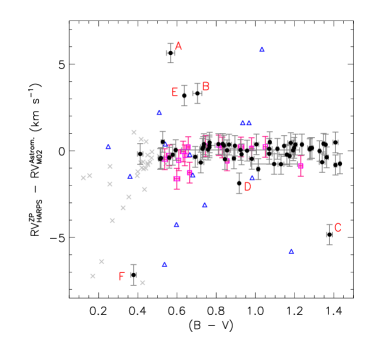
Figure 1: Difference $\Delta RV_{\rm M02}^{\rm ZP}$ between the spectroscopic RV corrected for zero point ($RV_{\rm HARPS}^{\rm ZP}$) and the astrometric RV ($RV_{\rm M02}^{\rm Astrom.}$) from M02 vs. $B-V$ for all the stars observed with HARPS. $RV_{\rm HARPS}^{\rm ZP}$ refers the HARPS RV measurements corrected for the zero point of 102 m s^-1 (see text). Its range is truncated for a close view of the data, and all stars beyond the bounds are binaries or have bad quality CCFs. Different symbols refer to quality classification: filled black circles for the selected data; grey crosses for the bad quality CCFs; blue triangles for spectroscopic binary stars (identified from the literature or from visual inspection of the CCFs); and purple squares for known BY Dra stars. Targets A–F are potential outliers described in Sect. 3. The magnitude $V$ and the $(B-V)$ color are from P98 and all stars shown fulfill the membership criterion of this work.

M02 sample was carefully selected for Hyades members that share the space velocity of the cluster with a low velocity spread. Out of the 168 stars in the M02 list, 131 were observed with HARPS. They constitute our initial sample since they have both, HARPS spectroscopic RV and M02 astrometric RV. After cleaning the M02 sample, we computed the G17 RVs for the finally selected stars.

When comparing spectroscopic and astrometric RV, we would expect, in the ideal case, a gaussian distribution. The centre representing the agreement between the two measurements and the dispersion of the distribution showing the velocity dispersion of the cluster (plus other sources of measurement noise). The cluster velocity dispersion should in fact dominate the width of the difference, because it will affect the spectroscopic RVs, but not the astrometric ones. The Hyades velocity dispersion is evaluated around 300–320 m s^-1 (P98; Reino et al. 2018).

The difference $\Delta RV_{\rm M02}^{\rm ZP}$ between the spectroscopic RV corrected for zero point (see Sect. 3.1), namely $RV_{\rm HARPS}^{\rm ZP}$, and the astrometric RV from M02, namely $RV_{\rm M02}^{\rm Astrom.}$, for the 131 sample stars is shown in Fig. 1. Different symbols indicate the quality of the fits, the binarity or stars with variable RV. Note that this Figure is limited to a $\sim\pm$ 7 km s^-1 range and several stars lay beyond these limits. This figure is equivalent and very similar to Fig. 4 of M02. The distribution of $\Delta RV_{\rm M02}^{\rm ZP}$ has an average value of $-2.0$ km s^-1, and a very broad standard deviation ($\sigma$) of 8.5 km s^-1. It is noticeable that many stars have a $\Delta RV_{\rm M02}^{\rm ZP}$ of several km s^-1, in large excess of the expected measurement errors and that the bulk of the sample is centred in a well defined sequence close to zero.

In order to have a more useful comparison, we cleaned the original sample from all the spectroscopic RV variables, such as known spectroscopic binaries and Delta Scuti stars. Several studies investigated binaries in the Hyades, in particular Griffin et al. (1988); Griffin (2012) summarise the results of many years of spectroscopic monitoring, identifying a number of spectroscopic binaries, which were first eliminated from the sample. Spectroscopic RVs of Delta Scuti stars are also known to vary by several km s^-1 (Poretti, 2001; Poretti et al., 2009) and these variables were also eliminated from the comparison.

In addition, the CCF peaks of some of the stars observed with HARPS are double, indicating that they are spectroscopic binaries. These stars (labelled as “SB” in the quality flag of table 1) were also removed. Finally a number of stars simply show rather bad CCFs. All of them are hot stars and the bad CCF profile is likely caused by the mismatch between the G2 mask and their early spectral types. We removed them as well from the final sample, although their exclusion or inclusion does not change substantially our main results. The likely single stars with bona fide CCFs (61 stars with flags 0 or 1 in Table 1) and the BY Dra variables (16 stars with “BY” flag) form our best sample, for a total of 77 stars. Not surprisingly, they concentrate around the solar-type region of the C-M diagram and cooler.

The mean difference $\Delta RV_{\rm M02}^{\rm ZP}$ for this sample is of $-101$ m s^-1 with a rather large spread, with $\sigma$ of 1.4 km s^-1. In fact, in spite all the known spectroscopic RV variables have been eliminated from the sample, a few stars show large spectroscopic – astrometric differences (larger than 2 km s^-1) (cf. Fig. 1); we searched in literature for more information on these stars and for all of them but one there is evidence for binarity or doubtful membership. Only for star (F) HIP 20614 we do not find any indication of binarity, however we notice that for this star the HARPS RV and the RV published by P98 differ by 5 km s^-1, indicating that its RV varies in the long period. We provide below a short summary of the stars with large spectroscopic and astrometric differences which have been discarded from our best sample.

• (A) HIP 10672. This star has a metallicity of $[Fe/H]=-0.12$ dex according to Paulson et al. (2004). In addition, the HARPS RV deviates from the published RV values.

• (B) HIP 13600. Chemical abundances deviate from those of the Hyades (Paulson et al., 2003). Therefore, this object is likely a nonmember.

• (C) HIP 16548 and (D) 16908. Both stars in the paper by Guenther et al. (2005) have low luminosity companion, about 3 mag fainter. One has a separation of 0.7 arc sec, one of 2.7.

• (E) HIP 19365. Given as potential binary in Simbad.

• (F) HIP 20614. Nothing special identified in different works (Hartkopf et al. 2001; Böhm-Vitense et al. 2002; P98), and no companion detected by speckle interferometry (Mason et al., 2009). Given the difference with previously published RV, we argue that also this star is a long period spectroscopic binary.

After removing these outliers, 71 objects are left. The average difference between spectroscopic (corrected for zero point) and astrometric RVs as measured from HARPS and Hipparcos (M02), namely $\Delta RV_{\rm M02}^{\rm ZP}$, is of $-85$ m s^-1, with a $\sigma$ of 464 m s^-1. The distribution of $\Delta RV_{\rm M02}^{\rm ZP}$, displayed in Fig. 2, is non gaussian, and the median is of +48 m s^-1. It is intriguing that this distribution is not gaussian, but skewed and possibly double-peaked. We discuss in Sect. 3.3 different possibilities for the origin of such asymmetry.

A cross-match between our final sample of 71 objects and the Gaia Archive results in a subsample of 65 objects with new astrometric data, including parallax. The astrometric RV can also be computed for the missing 6 objects by using equatorial coordinates from another catalogue in Eq. (2) of M02. We used the Hipparcos coordinates, which differ by typically $\sim 3$ arcsec from the Gaia values. This difference is negligible in the astrometric RV calculation. The distribution of the spectroscopic (from HARPS, corrected for zero point) minus astrometric RVs from G17, namely $\Delta RV_{\rm G17}^{\rm ZP}$, is similar to the $\Delta RV_{\rm M02}^{\rm ZP}$ distribution displayed in Fig. 2, just shifted by an offset. Therefore, the asymmetry of the $\Delta RV_{\rm M02}^{\rm ZP}$ distribution is also observed in the $\Delta RV_{\rm G17}^{\rm ZP}$ distribution. The $\sigma$ value of the $\Delta RV_{\rm G17}^{\rm ZP}$ distribution is 462 m s^-1, similar to the $\sigma$ of $\Delta RV_{\rm M02}^{\rm ZP}$.

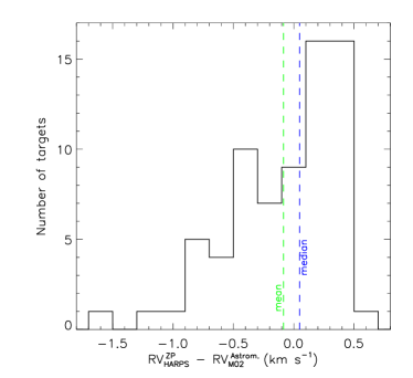
Figure 2: Distribution of the spectroscopic – astrometric RV differences (corrected for zero point), $\Delta RV_{\rm M02}^{\rm ZP}$, for the M02 astrometric solution for the best quality subsample (of 71 stars with flags 0, 1, and “BY”, and outliers excluded). The mean and median values of the distribution are illustrated by the green and blue dashed lines, respectively.

3.1 Accuracy of spectroscopic RV

Most spectroscopic RV applications (e.g. clusters membership, search for binaries or exo-planets) are interested in obtaining the highest measurements precision. The present study, that compares results obtained with different techniques, requires as well a high accuracy.

The zero point of the G2 mask of HARPS has been measured to an accuracy of a few m s^-1, by comparing spectroscopic RV and true velocities of solar system bodies, by Lanza et al. (2016), who find a (relativistic corrected) shift that varies between 98 and 102 m s^-1, correlating with the solar activity cycle. Our observations were taken in December 2014, in a period not included in the Lanza et al. study; however, since in the last years of the Lanza study the zero point of the HARPS G mask has been rather stable with time, we consider a zero point of 102 m s^-1 appropriate for our observations. This zero point correction must therefore be added to all the data of Table 1. We shall keep in mind that an additional, systematic uncertainty of $\pm$2 m s^-1 is associated to our HARPS observations when performing the zero point correction because of its uncertainty. For most spectra the formal error to the fit of the HARPS CCF is smaller than this zero point uncertainty. We also note that after the change of HARPS fibres to octagonal ones, the zero point of the G2 HARPS mask has moved by further $\sim$12 m s^-1 (Lo Curto et al., 2015; Molaro et al., 2016).

Other aspects of stellar physics affect the spectroscopic RV accuracy (see Lindegren & Dravins, 2003). Stellar activity, for instance, may contribute with two effects. The first effect is that rotating inhomogeneities on stellar surface or long-term activity cycles distort the spectral line profiles, producing shifts in the observed RVs of individual targets. However, the shifts are modulated with time, and by observing many stars we shall cover random rotation or activity-cycle phases. The net result is that we do not expect a systematic shift from this effect; rather an extra jitter in the spectroscopic radial velocity distribution, that will add to the cluster velocity dispersion (but it is almost one order of magnitude smaller). It is not easy to evaluate the RV variability introduced by activity, but several authors estimate that jitter to less than 40 m s^-1 for the Hyades (Paulson et al., 2004; Saar & Donahue, 1997). The second effect of activity may, instead, introduce a systematic shift, because all the Hyades cluster stars are enhanced in activity with respect to the Sun, and all our zero point corrections, either empirical or theoretical, are suitable for a quiet star. These (and other) effects are separately discussed in Sect. 4.

3.2 Accuracy of astrometric RVs

The difference between the M02 and G17 RVs is dominated by the offset caused by the different cluster space velocity found by the two authors. Being the astrometric radial velocities the projection of the coordinates vector on the space velocity vector, the use of a different space velocity translates into an offset, which is of $\left<RV_{\rm G17}-RV_{\rm M02}\right>=-123$ m s^-1, with a narrow $\sigma$ of 8 m s^-1 for our case.

The formal errors for the astrometric RV computed in M02 are given by Lindegren et al. (2000) and are of the order of 600 m s^-1. We must be careful on the interpretation of these astrometric uncertainties, because M02 mention that their alternative solution, based of Tycho values, has an offset of $-900$ m s^-1 with respect to the Hipparcos one. Similarly, van Leeuwen (2009) proposes a space motion for the Hyades that is also about 1 km s^-1 lower than the M02 one. The de Bruijne et al. (2002) solution as well as most solutions quoted in his paper and based on Hipparcos results, are compatible with M02. In their Table 1 de Bruijne (2001) compare the Hyades space motions derived in several studies, and the majority predicts an astrometric RV for the cluster between 39.44 and 39.51 km s^-1 (70 m s^-1 span); only the P98 and the Van Leeuwen solutions (plus the Tycho 2 solution of M02) form a distinct group, all providing a cluster RV about 1 km s^-1 smaller. These discrepancies should induce some caution in (over-) interpreting the results. The comparison with the Gaia solution is however reassuring, because the M02 Hipparcos solution and the Gaia G17 RVs agree to $\sim$120 m s^-1.

3.3 The cluster rotation

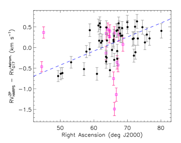
Figure 3: Spectroscopic – astrometric G17 RV differences (corrected for zero point), $\Delta RV_{\rm G17}^{\rm ZP}$, vs. right ascension ($\alpha$) for our stars. Dashed blue line is a linear fit (computed by excluding the BY Dra variables; see text) illustrating the correlation between these quantities. Target symbols and colours follow the same description as in Fig. 1.

In order to understand the origin of the asymmetry and the overall shape of the $\Delta RV_{\rm M02}^{\rm ZP}$ and $\Delta RV_{\rm G17}^{\rm ZP}$ distributions, we have looked at the dependence of $\Delta RV_{\rm G17}^{\rm ZP}$ on several parameters. The same analysis can be repeated with the M02 data, and provides same results, but with higher uncertainties. Most significant is the correlation between $\Delta RV_{\rm G17}^{\rm ZP}$ and the stars’ right ascension ($\alpha$), as shown in Fig. 3. The Pearson correlation coefficient of this plot is 0.35 for all the 71 targets and 0.56 if we remove the BY Dra variables (purple squares), which show a larger noise than the rest of the sample. A linear fit without considering the BY Dra variables gives that $\Delta RV_{\rm G17}^{\rm ZP}$ increases with $\alpha$ by $\sim$34 m/s/deg: $\Delta RV_{\rm G17}^{\rm ZP}=(0.0340\pm 0.0032)\alpha-(2.12\pm 0.21)$ km s^-1 (dashed blue line in the figure). A much weaker correlation for the declination ($\delta$) is also present in the data, but this is because $\alpha$ and $\delta$ are not fully independent. When $\Delta RV_{\rm G17}^{\rm ZP}$ is corrected for the $\alpha$ dependence, no correlation of $\Delta RV_{\rm G17}^{\rm ZP}$ with $\delta$ is left.

We tested and excluded two hypotheses that could explain such a dependence of $\Delta RV_{\rm G17}^{\rm ZP}$ with the target coordinates: inaccurate velocity vector and cluster expansion. The tests consisted of several trials of a simple Hyades model based on the derived parameters for its 3D position and space velocity. For the first hypothesis, we let the the velocity vector components free, in order to minimize the correlation between $\Delta RV_{\rm G17}^{\rm ZP}$ and $\alpha$. Because the changes in velocity should be greater than 1 km/s for such a minimization, we consider this cause unlikely. For the cluster expansion, we verified that adding a radial expansion velocity for the cluster does produce an asymmetry in the RV distribution. However, that velocity should be much larger than the upper limit of 70 m s^-1 estimated for the Hyades (see Sect. 4.3) to reproduce the observed distribution of $\Delta RV_{\rm G17}^{\rm ZP}$. We therefore also discarded this possibility.

A natural way of producing the $\Delta RV_{\rm G17}^{\rm ZP}$ dependence on $\alpha$ rotation of the cluster. Intuitively, a cluster rotation should naturally produce a dependence of RV with star position, possibly a double peak in the RV distribution, and a skewness if the observed stars are not distributed homogeneously with respect to the cluster center. We can convert the dependence on $\alpha$ into velocity gradient by assuming a distance of the cluster center at 46.09 parsecs (Reino et al., 2018), obtaining a rotation of 42.27 m s^-1 pc^-1.

We note that Vereshchagin & Chupina (2013) found indications of cluster rotation, with a gradient similar to ours, but with low statistical significance. More recently, Reino et al. (2018), based on GAIA DR2, concluded that the astrometric data alone do not support a significant rotation of the cluster. Our results provide evidence that the Hyades cluster rotates and therefore the comparison between spectroscopic and astrometric RV requires a correction for cluster rotation in the astrometric model.

4 Phenomena affecting spectroscopic and astrometric RV

4.1 Gravitational redshift

Gravitational redshift has been predicted by Einstein (1917). The GR effect scales with the solar mass and radius according to

$$\Delta RV_{GR}=636.5\times(M/R)-3.0\rm{~{}~{}m~{}s}^{-1}$$ (2)

(for $M$ and $R$ given in Solar units), where the first term is the redshift as the light emitted from the solar photosphere was observed from infinity and the second term is the correction by placing the observer at the mean Earth distance from the Sun (e.g., Lindegren & Dravins, 2003). Since the ratio $M/R$ may change easily by a factor 10 in an open cluster when comparing main sequence and giant stars (the effect is much larger for white dwarfs, but they are not studied here), this is a very relevant effect, because spectroscopic RV are affected by GR, while astrometric ones are not. The measurement of GR in the Sun is not trivial, and several attempts have shown a general agreement with the Einstein prediction, but with a limited accuracy (Beckers, 1977). Pasquini et al. (2011) studied spectroscopic RVs for many stars with different masses and radii in the open cluster M67, but did not find evidence for GR. They used 3D atmospheric models to simulate lines of different equivalent widths in giants and dwarfs, finding that the lines in the dwarfs are blue-shifted with respect to giant stars by an amount that largely compensates the differential GR. M67 is of solar chemical composition Randich et al. (2000), while the Hyades are metal rich (Dutra-Ferreira et al., 2016). The instrument and mask used by Pasquini et al. (2011) were also different from the one adopted here.

We estimated GR by computing the $M/R$ for each star, as described in Sect. 2.3. The GR and $M/R$ values are given in Table 2 together with other parameters that are described below. An analysis of the spectroscopic – astrometric RV differences allows us to measure the GR effect from our data. This analysis is presented in Sect. 5.

4.2 Convective line shifts

Convective blue shifts in stars are expected to be a major contributor to spectroscopic RVs, at a level comparable with GR, and being of opposite sign to GR, they will partially compensate for this effect.

Using a recent library of synthetic spectra based on hydrodynamical model atmospheres (Ludwig et al., 2017) we estimated convective line shifts for 75 stars of our “best” sample (two stars were too hot to be covered by the model calculations). This was done by cross-correlating the synthetic spectra with the G2-mask applied in the HARPS data reduction pipeline (Pepe et al., 2002). Effects of the finite spectral resolution of HARPS and stellar rotation were taken into account (see Appendix A for details). The predicted shifts are listed in Table 2.

We emphasize that the listed values are the results of the synthetic profiles convolved with the HARPS mask, so, while they are appropriate for the present work and for HARPS observations in general, they should not be taken as absolute values of the convective line shift in the particular star.

As sanity check we compared predicted shifts to the velocity zero point of +102 m s^-1 measured for the solar spectrum with HARPS by Lanza et al. (2016). We used reduced spectra provided at the ESO webpage (Collection of HARPS solar spectra) of Ceres, Ganymede, the Moon, and a daylight solar spectrum to estimate the full width at half maximum (FWHM) of the cross-correlation as observed by HARPS. Our calculations gave an FWHM of $7.2\pm 0.1$ km s^-1 for Ceres, Ganymede, and the Sun and $7.4\pm 0.1$ km s^-1 for the Moon. For the 7.2 km s^-1 width, we get a predicted shift for the solar spectrum of $-490.2$ m s^-1. Assuming a solar gravitational redshift of $+633.5$ m s^-1 this results in a total zero point correction of $+143.3$ m s^-1, to be compared to the value of Lanza and collaborators of $+102$ m s^-1. The difference of $41.3$ m s^-1 is within the numerical accuracy we expect for the theoretical spectra reflecting the underlying kinematics of flows in the 3D model atmospheres. Further possible sources of uncertainties are: wavelengths errors in the line list applied in the spectral synthesis, neglect of departures from local thermodynamic equilibrium in the spectral synthesis, and shortcomings of our approximate cross-correlation procedure when comparing to pipeline results. However, in view of the modest velocity offset found, we consider the correspondence satisfactory.

Having checked that the models provide sensible results for the Sun, we have applied the theoretical corrections for the two dominant effects, GR and convection, to all the stars, and the $\Delta RV_{\rm M02}^{GR+C}$ and $\Delta RV_{\rm G17}^{GR+C}$ values (the $GR+C$ superscript means corrected for GR and convection) so found are tabulated in Table 2. An analysis of these corrections is presented in Sect. 5.

Table 2: Gravitational and convective shifts.

#	HIP	$M/R$	$GR$	$C$	$GR+C$	$\Delta RV_{\rm M02}$	$\Delta RV_{\rm M02}^{GR}$	$\Delta RV_{\rm M02}^{GR+C}$	$\Delta RV_{\rm G17}$	$\Delta RV_{\rm G17}^{GR}$	$\Delta RV_{\rm G17}^{GR+C}$
			(m s-1)	(m s-1)	(m s-1)	(m s-1)	(m s-1)	(m s-1)	(m s-1)	(m s-1)	(m s-1)
2	16529	1.130 $\pm$ 0.041	716	-340	377	-383	-1100	-760	-255	-972	-632
4	18327	1.135 $\pm$ 0.046	720	-318	402	391	-329	-11	523	-197	121
5	19098	1.135 $\pm$ 0.077	719	-327	392	-341	-1061	-733	-214	-934	-606
6	19148	1.061 $\pm$ 0.070	672	-563	109	142	-530	33	269	-404	160
8	19781	1.097 $\pm$ 0.061	696	-449	246	-249	-945	-495	-121	-816	-367
9	19796	1.028 $\pm$ 0.052	651	-573	79	-368	-1020	-447	-236	-888	-315
10	20146	1.106 $\pm$ 0.048	701	-451	250	-574	-1275	-823	-447	-1147	-696
11	20205	0.248 $\pm$ 0.015	155	-566	-412	-362	-516	50	-241	-396	170
12	20480	1.115 $\pm$ 0.050	707	-389	318	171	-535	-146	289	-418	-29
13	20492	1.132 $\pm$ 0.064	717	-340	378	128	-590	-250	252	-465	-126
14	20557	1.030 $\pm$ 0.041	652	-602	51	-316	-969	-367	-196	-849	-247
16	20826	1.047 $\pm$ 0.039	663	-615	48	-296	-960	-345	-171	-834	-219
17	20850	1.130 $\pm$ 0.056	716	-345	371	404	-312	33	523	-193	152
18	20889	0.220 $\pm$ 0.013	137	-562	-425	-955	-1092	-530	-838	-975	-413
19	20949	1.117 $\pm$ 0.051	708	-392	315	577	-131	262	689	-18	374
20	20978	1.133 $\pm$ 0.038	718	-313	406	461	-257	55	584	-134	179
21	21099	1.109 $\pm$ 0.064	703	-413	290	321	-382	30	442	-261	151
22	21741	1.125 $\pm$ 0.059	713	-391	322	486	-227	164	599	-115	277
23	22380	1.129 $\pm$ 0.043	716	-355	360	496	-220	136	608	-108	247
24	22422	1.054 $\pm$ 0.053	668	-623	45	-127	-795	-172	-11	-680	-56
25	22566	1.034 $\pm$ 0.048	655	-617	38	618	-37	580	736	81	698
26	23069	1.110 $\pm$ 0.060	703	-396	308	484	-219	177	595	-109	287
27	23498	1.116 $\pm$ 0.063	708	-408	299	302	-405	3	417	-291	117
28	23750	1.108 $\pm$ 0.078	702	-438	264	215	-487	-49	324	-378	60
29	24923	1.116 $\pm$ 0.063	708	-410	297	406	-301	109	506	-201	209
31	15300	1.016 $\pm$ 0.077	644	-289	355	-719	-1362	-1074	-589	-1233	-944
32	15563	1.119 $\pm$ 0.033	709	-236	473	-674	-1383	-1147	-532	-1241	-1005
33	15720	1.003 $\pm$ 0.080	636	-286	350	-645	-1281	-995	-516	-1152	-866
35	17766	1.049 $\pm$ 0.050	665	-243	422	-557	-1222	-980	-421	-1086	-843
36	18018	1.112 $\pm$ 0.087	705	-229	476	-118	-823	-593	4	-701	-471
37	18322	1.129 $\pm$ 0.056	716	-236	480	-75	-791	-554	63	-652	-416
38	18946	1.126 $\pm$ 0.079	713	-236	478	-663	-1377	-1141	-535	-1249	-1013
39	19082	1.046 $\pm$ 0.118	663	-230	433	510	-153	77	637	-26	204
40	19207	1.107 $\pm$ 0.056	702	-234	467	556	-146	89	689	-13	221
41	19263	1.136 $\pm$ 0.065	720	-260	460	473	-247	13	598	-122	138
42	19316	1.055 $\pm$ 0.144	669	-273	396	89	-579	-307	220	-449	-176
43	19441	1.104 $\pm$ 0.062	700	-231	469	126	-574	-343	262	-437	-206
44	19808	1.100 $\pm$ 0.065	697	-231	466	461	-236	-5	590	-108	124
45	19834	1.039 $\pm$ 0.075	658	-351	307	-275	-934	-582	-144	-802	-451
46	19862	1.137 $\pm$ 0.227	721	-286	434	150	-571	-284	273	-448	-161
47	20357	0.983 $\pm$ 0.046	622	-522	101	-82	-704	-182	44	-579	-57
48	20527	1.072 $\pm$ 0.080	679	-236	443	263	-416	-180	384	-295	-59
49	20605	1.016 $\pm$ 0.110	644	-312	332	585	-58	254	707	63	375
50	20745	1.041 $\pm$ 0.053	660	-245	415	456	-204	41	586	-74	171
51	20762	1.116 $\pm$ 0.061	707	-236	472	381	-326	-90	508	-199	36
52	20827	1.137 $\pm$ 0.085	721	-333	388	-101	-822	-489	17	-703	-370
53	21138	1.075 $\pm$ 0.161	681	-234	447	261	-420	-187	385	-297	-63
54	21256	1.090 $\pm$ 0.079	691	-239	452	464	-227	11	575	-116	123
55	21261	1.102 $\pm$ 0.060	699	-234	465	273	-426	-192	388	-311	-77
56	21723	1.129 $\pm$ 0.061	716	-237	478	599	-116	121	717	1	239
57	22177	1.076 $\pm$ 0.071	682	-237	444	190	-492	-254	310	-372	-134
58	22253	1.123 $\pm$ 0.084	712	-248	463	216	-496	-247	324	-388	-140
59	22271	1.109 $\pm$ 0.051	703	-224	478	-200	-903	-678	-94	-796	-572
60	22654	1.129 $\pm$ 0.075	716	-248	468	216	-500	-252	322	-394	-146
61	23312	1.137 $\pm$ 0.106	721	-309	412	110	-611	-302	226	-495	-186
62	13806	1.132 $\pm$ 0.037	717	-318	399	-484	-1201	-883	-362	-1079	-761
63	13976	1.137 $\pm$ 0.060	721	-292	429	323	-397	-106	467	-253	38
64	19786	1.080 $\pm$ 0.071	684	-514	171	-162	-846	-333	-31	-715	-201

Notes. Columns are HIP: Hipparcos number; $M/R$: stellar mass over radius in solar units; $GR$: estimated gravitational redshift; $C$: estimated convective shift; $GR+C$: gravitational plus convective shift; $\Delta RV_{\rm M02}$: RV difference between HARPS (without zero point correction) and M02 measurements; $\Delta RV_{\rm M02}^{GR}$: $\Delta RV_{\rm M02}$ corrected from $GR$; $\Delta RV_{\rm M02}^{GR+C}$: $\Delta RV_{\rm M02}$ corrected from $GR+C$. $\Delta RV_{\rm G17}$: RV difference between HARPS (without zero point correction) and G17 measurements; $\Delta RV_{\rm G17}^{GR}$: $\Delta RV_{\rm G17}$ corrected from $GR$; $\Delta RV_{\rm G17}^{GR+C}$: $\Delta RV_{\rm G17}$ corrected from $GR+C$.

Table 2: Continued.

#	HIP	$M/R$	$GR$	$C$	$GR+C$	$\Delta RV_{\rm M02}$	$\Delta RV_{\rm M02}^{GR}$	$\Delta RV_{\rm M02}^{GR+C}$	$\Delta RV_{\rm G17}$	$\Delta RV_{\rm G17}^{GR}$	$\Delta RV_{\rm G17}^{GR+C}$
			(m s-1)	(m s-1)	(m s-1)	(m s-1)	(m s-1)	(m s-1)	(m s-1)	(m s-1)	(m s-1)
65	19793	1.086 $\pm$ 0.057	688	-520	168	321	-367	153	444	-244	276
66	19934	1.126 $\pm$ 0.042	714	-353	361	419	-294	58	544	-170	183
67	20082	1.137 $\pm$ 0.067	721	-283	438	249	-472	-190	374	-347	-64
68	20130	1.112 $\pm$ 0.052	705	-384	321	378	-327	57	498	-207	177
69	20237	1.047 $\pm$ 0.045	663	-596	68	-164	-827	-231	-41	-704	-109
70	20485	1.092 $\pm$ 0.083	692	-235	457	-771	-1463	-1228	-651	-1343	-1109
71	20563	1.132 $\pm$ 0.076	718	-256	461	330	-388	-131	449	-268	-12
72	20577	1.063 $\pm$ 0.252	674	-581	93	-1513	-2187	-1606	-1388	-2062	-1481
73	20741	1.088 $\pm$ 0.066	690	-514	175	-1161	-1850	-1336	-1039	-1728	-1214
74	20815	1.038 $\pm$ 0.039	658	-615	43	-383	-1041	-426	-256	-914	-299
75	20899	1.068 $\pm$ 0.058	677	-567	109	-445	-1122	-555	-323	-1000	-432
76	20951	1.129 $\pm$ 0.079	715	-318	397	292	-423	-105	416	-300	19
77	21317	1.076 $\pm$ 0.066	682	-523	159	59	-623	-100	177	-505	18

4.3 Cluster expansion

Dravins et al. (1999) pointed out that the astrometric RV are computed neglecting the hypothesis that the cluster may be expanding in the present, and under the assumption of constant expansion with time, this would provide for the Hyades an upper limit of 70 m s^-1. This implies that if cluster expansion did occur, the measured astrometric RVs should be systematically larger than the ones without expansion by up to this amount. This implies that $\Delta RV_{\rm ZP}$ could be upper limits as far as this effect is concerned.

4.4 Stellar activity

As mentioned in Sect. 3.1, enhanced stellar activity may induce a systematic effect, that is not considered in the zero point corrections. Lanza et al. (2016) observed that the HARPS RV of the Sun redshifts by a few m s^-1 when activity increases with the 11 years solar cycle. This effect, if extrapolated to active stars as the Hyades, would produce a systematic redshift of the stellar lines. Note that this is not the RV Jitter induced by chromospheric variable activity on, e.g., a rotational period, that we assume will average out by observing many stars. The spectra of all the stars would be systematically shifted because, assuming that the active stars are dominated by structures similar to those producing the 11 yrs solar cycle, the photospheric lines are systematically redshifted with respect to the Sun (our zero point reference), that is a relatively quiet and old star.

All the RV studies we are aware of show a correlation between activity and spectroscopic redshift, although a direct link between activity indicators and shifts is not always present (Dumusque et al., 2012; Lovis et al., 2011; Lanza et al., 2016). The chromospheric activity level of the Hyades solar stars is about 4–5 times higher than the Sun (Pace & Pasquini, 2004). If we consider that the Sun varied by $\sim$4 m s^-1 peak to peak over the last cycle (with a corresponding chromospheric activity variation of $\sim 40\%$ as measured from the CaII Index, Lanza et al. 2016), and assuming a linear relationship between RV redshift and the Logarithm of the Calcium H and K chromospheric flux, as found by Dumusque et al. (2012) for $\alpha$ Cen B, we would expect that Hyades spectral RVs are affected by a systematic zero point redshift of less than $\sim$ 50 m s^-1. At present we cannot establish a precise value for this shift, also because the magnetic structures (chromospheric network, plages, spots) contribute differently to the shift (Haywood et al., 2016), and we do not know in detail which structures are present on the surface of these stars.

4.5 Stellar rotation

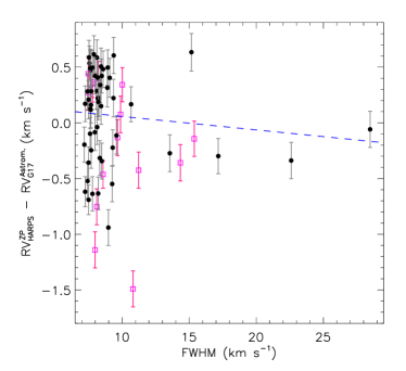
Figure 4: Difference between the spectroscopic and astrometric RV as a function of FWHM for our stars. Symbols and colours follow the same definition as in Fig. 1. Dashed blue line is a linear fit with the data (excluded the BY Dra variables).

One motivation for this study was the hint in M02 that the difference between astrometric and spectroscopic RVs might depend on stellar rotation. Lindegren & Dravins (2003) discuss the effects of enhanced rotation on spectroscopic RV measurements and argue that some spectral lines could shift as much as hundreds of m s^-1. We used as a proxy of the stellar rotational velocity the FWHM of the CCF, which is expected to be almost linearly related to the projected rotational velocity $v\sin i$ (e.g., Geller et al., 2010). Figure 4 shows this analysis within the FWHM span of our final sample, between 6 and 30 km s^-1. The Pearson correlation of this distribution (excluding BY Dra variables) is low (-0.13) and a linear fit with the data, showed by the dashed blue line, gives:

$$\Delta RV_{\rm G17}^{\rm ZP}=-(0.012\pm 0.006)\times{\rm FWHM}+(0.18\pm 0.06){\rm~{}~{}km~{}s}^{-1},$$

which decreases slightly for increasing FWHM. The relatively small slope (with 50% uncertainty) may be caused by a selection effect because it is mainly produced by the fast rotators, which have a sparse distribution and relatively high spread. Indeed, the slope changes to $3\pm 3$ m s^-1 if we compute another linear fit for a restricted range of FWHM $<$ 12 km s^-1, where the Pearson correlation is almost null (0.02). We do not find therefore any measurable effect of rotational velocity on RV measurements in the range of stars studied, though some variations, dependent on the spectral type of the stars, is expected from our 3D models.

4.6 Relativistic corrections

All the spectroscopic RV should be in principle corrected for a relativistic effect. One can estimate (e.g., Lindegren & Dravins, 2003) that the difference between the spectroscopic and astrometric RV measurements is given by

$$\left|RV_{\rm Spectr.}-RV_{\rm Astrom.}\right|\approx\frac{RV^{2}}{2c},$$

with $RV$ representing the ideal value free from any effect. Considering an average RV of the cluster stars of 39.4 km s^-1, this would imply a typical correction of $\sim$2.6 m s^-1, that can be considered negligible with the present level of accuracy. The relativistic correction for the transversal motion ($\sim$29 km s^-1) provides similar values.

4.7 Galactic gravitational potential

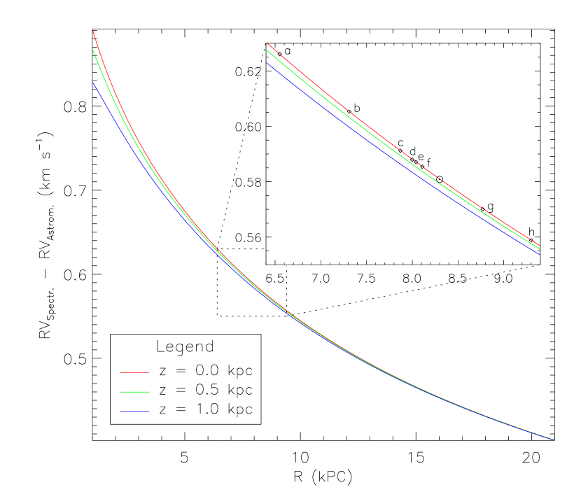
Figure 5: The expected effect of the Galactic potential on the difference between the spectroscopic and astrometric RV measurements as a function of the cylindrical coordinates $R$ and $z$ with the origin at the Galactic centre. A close view of the solar neighborhood is depicted in the subpanel at the upper right region of the figure. A small list of clusters selected from Dravins et al. (1999) is shown in this subpanel by the letters “a” to “h”. These are (a) NGC 6618, (b) IC 4725, (c) Upper Scorpius, (d) Coma Berenices, (e) Hyades, (f) Pleiades, (g) NGC 7789, and (h) NGC 2099. The Sun is illustrated by the solar symbol.

The difference between astrometric and spectroscopic RV will also depend on the gravitational potential of the Galaxy, or better on the difference between the Galactic potential at the position of the observed star and of the sun. In principle, if our measurement were accurate enough, the comparison between astrometric and spectroscopic RV should trace the Galactic potential. This difference is given by just GR, so it will depend on (M/R), where here M and R refer to the Mass and Radius of the Galaxy at the stellar position and at the solar position; such an effect will be very small for nearby stars, but it may be of several hundreds of m s^-1 close to the bulge on in the MCs as pointed out by Lindegren & Dravins (2003).

Gravitational redshift due to the Galactic potential will only affect the spectroscopic measurements, not the astrometric ones. In other words, the same cluster, observed at 7 kpc distance towards the centre and the anti-centre, would show difference between spectroscopic and astrometric RVs of about 0.5 km s^-1. This can be seen clearly in Fig. 5, in which we used a model of the Galactic potential (Piffl, 2014) to compute the expected effect. In the same figure we position a number of open clusters for which astrometric RV could be in principle obtained by a precise astrometric mission, such as Gaia. The maximum difference is of about 60 m s^-1, which would be easily measurable as far as spectroscopic velocities are concerned, in particular if stars of similar spectral type were observed in the two clusters. We note, however, that to estimate accurately the valocity vector is not trivial, even for a nearby cluster as the Hyades (the reported G17 uncertainty is of 120 m s^-1) and, in addition, that for the further clusters the astrometric precision will be lower and may not be sufficient even with Gaia. For some of the clusters, cluster expansion effect may also become relevant. Dravins et al. (1999) compiled a list of open clusters that could be characterized by a Gaia-type mission and only for three the velocity vector should be meaurable to better than 100 m s^-1. As far as the Hyades are concerned, with a distance from the sun of 46.5 parsec (van Leeuwen, 2007) and a radial distance of ${8\,042.6}$ parsec the expected redshift produced by the galactic potential is of 587 m s^-1, whereas for the Sun it is of 581 m s^-1, which gives a systematic difference of only 6 m s^-1.

5 Gravitational redshift and convection

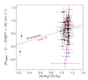
Figure 6: Difference between the spectroscopic (corrected for convective shifts) and astrometric (corrected for cluster rotation) RV as a function of $M/R$ for the 71 stars of our sample. Target symbols and colours follow the same description as in Fig. 1. The grey dotted line depicts the theoretical prediction of the GR from Eq. (2). The red dashed line is a linear fit to the observed data, excluding the BY Dra variables.

As introduced in the previous sections, GR and convection (described in Sects. 4.1 and 4.2 respectively) are the two effects that dominate the distortions in spectroscopic RV measurements. Even if the two effects are comparable and have opposite sign, we do not expect that they cancel completely, as can be seen from the theoretical values given in Table 2.

As shown above, the Hyades cluster rotates, and this effect has not been taken into account in the astrometric measurements. In order to be consistent and to perform a detailed analysis, we have added to the astrometric velocity of our 71 stars the contribution of cluster rotation, using the gradient found in Sect. 3.3. Hipparcos parallaxes were used for the 6 targets with missing G17 parallaxes.

If we correct $\Delta RV_{\rm G17}$ (the simple difference between measured HARPS and G17 astrometric velocities) for cluster rotation (CR) and for the convective shift, the resulting RV difference, namely $\Delta RV_{\rm G17}^{C+CR}$, is expected to be dominated by GR, which can thus be determined empirically. Figure 6 shows $M/R$ versus $\Delta RV_{\rm G17}^{C+CR}$ for our 71 stars. The two Hyades giants show smaller $\Delta RV_{\rm G17}^{C+CR}$ than the average of the other stars, as expected by GR because of their substantially smaller $M/R$. A linear fit of $M/R$ versus $\Delta RV_{\rm G17}^{C+CR}$ data, excluded the BY Dra variables, provides:

$$\Delta RV_{\rm G17}^{C+CR}=(0.626\pm 0.131)\times(M/R)-(0.040\pm 0.140){\rm~{}~{}km~{}s}^{-1}.$$

The slope of $\Delta RV_{\rm G17}^{C+CR}$ of $626\pm 131$ m s^-1 agrees well with the theoretical prediction of GR (grey dotted line in Fig. 6), given by Eq. (2), within the uncertainty of the measurement. The 131 m s^-1 uncertainty is somewhat high because only two giants are part of our sample, and they are essential to extend the $M/R$ versus $\Delta RV_{\rm G17}^{C+CR}$ distribution to low $M/R$ values for computing and determine the GR slope.

We finally show the results of our best estimate for the comparison between astrometric and spectroscopic RVs in Fig. 7. The distribution represents, for the stars of our sample (excluding the BY Dra), the difference between the spectroscopic RVs (subtracted by the GR and convective contribution) and the astrometric G17 RVs (with the cluster rotation added). As anticipated in Sect. 3.3, introducing the cluster rotation brings the distribution close to a normal one. The mean difference is of $-33$ m s^-1, the median $-16$ m s^-1 with a $\sigma$ of $347$ m s^-1. This result shows quite a good agreement between spectroscopic and astrometric radial velocities, indirectly validating the steps and models used.

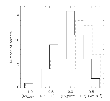
Figure 7: Solid line is the distribution of the difference between spectroscopic (corrected for convective shifts and gravitational redshift) and astrometric (corrected for cluster rotation) RV for 55 stars of our sample (the BY Dra have been excluded). The distribution is gaussian and centered very close to zero. Dashed line is the distribution of the RV difference for the same sample without correction for comparison (with a slight shift of +0.02 km s^-1 for better visualization), where there is a clear asymmetry as in Fig. 2.

Table 3: Summary of $\Delta RV$ results.

Major effects
	$GR$	$C$	$\Delta RV_{\rm M02}$	$\Delta RV_{\rm M02}^{\rm ZP}$	$\Delta RV_{\rm M02}^{GR}$	$\Delta RV_{\rm M02}^{GR+C}$	$\Delta RV_{\rm G17}$	$\Delta RV_{\rm G17}^{\rm ZP}$	$\Delta RV_{\rm G17}^{GR}$	$\Delta RV_{\rm G17}^{GR+C}$
	(m s-1)	(m s-1)	(m s-1)	(m s-1)	(m s-1)	(m s-1)	(m s-1)	(m s-1)	(m s-1)	(m s-1)
Mean	$678$	$-366$	$+17$	$-85$	$-661$	$-295$	$+139$	$+37$	$-538$	$-172$
Median	$+701$	$-327$	$+150$	$+48$	$-530$	$-189$	$+273$	$+171$	$-404$	$-64$
$\sigma$	$95$	$130$	$464$	$464$	$443$	$429$	$462$	$462$	$441$	$426$

Minor effects
Cluster	Stellar	General	Galactic
Expansion	Activity	Relativity	Potential
(m s-1)	(m s-1)	(m s-1)	(m s-1)
$>-70$	$<+50$	$<+3$ spectra	$+6$
		$<+3$ astro

Notes. The top panel shows the major effects affecting the RV measurements. Their mean and median values, and standard deviations are obtained from the data of Table 2. Columns named $GR$ and $C$ refers to the gravitational redshift and convective shift, as discussed in Sects. 4.1 and 4.2, respectively. $\Delta RV_{\rm M02}$ and $\Delta RV_{\rm M02}^{\rm ZP}$ refer to the HARPS minus M02 astrometric RV difference without and with zero point correction, respectively. Column $\Delta RV_{\rm M02}^{GR}$ shows the global shift on the $\Delta RV_{\rm M02}$ values when the GR contribution is subtracted, whereas $\Delta RV_{\rm M02}^{GR+C}$ gives $\Delta RV_{\rm M02}$ corrected for the two most relevant effects: GR and convective shift $C$. Columns from $\Delta RV_{\rm G17}$ to $\Delta RV_{\rm G17}^{GR+C}$ follow the same descriptions as those for columns $\Delta RV_{\rm M02}$ to $\Delta RV_{\rm M02}^{GR+C}$, but using the G17 astrometric RVs. The bottom panel shows the minor effects, discussed in Sects. 4.3, 4.4, and 4.6, respectively. A positive value means that the effect should be subtracted from $\Delta RV$, because it contributes positively to the difference, so either it adds a redshift to the spectroscopic measurement, or decreases the astrometric one.

6 Hyades RV

The latest Hyades RV in literature before G17 is $39.4\pm 0.6$ km s^-1 (Maderak et al., 2013), computed by averaging the RV of their sample. These authors also measured a median difference of $-0.56$ km s^-1 between their RV measurements and those published by P98, similar to our findings. G17 provide a new estimate of the Hyades RV of $39.38\pm 0.16$ km s^-1 (purely astrometric solution) computed from kinematic models.

The new HARPS measurements, coupled with our accurate zero points and the discovery of more double or RV variable stars, can be used to provide a new, accurate spectroscopic RV for this cluster, namely $RV_{\rm Hyades}^{\rm HARPS}$. To do this, we considered the 3D structure of the cluster by using the equatorial coordinates of the stars and G17 parallaxes. Then, we analyzed a few subsample selections of stars within a 3–10 pc radius from the cluster centre, namely between the cluster core and its tidal radius (Madsen, 2003). We used the Hyades central coordinates provided in G17. The two giants of our sample were excluded because the GR effect makes them to deviate from the dwarfs and then to bias our results. For each subsample selection, the stellar RVs corrected for zero-point were adjusted to their projection to the cluster centre, by $RV/\cos\theta$, where $\theta$ is the angular distance to the cluster centre. Since the projected RV distribution is not fully gaussian, but slightly asymmetric, we use the median value of the projected RVs as a suitable measure of $RV_{\rm Hyades}^{\rm HARPS}$.

The median value of the projected HARPS RVs tends to increase the smaller the subsample region is. The selection within the tidal radius ($<$10 pc, comprising 46 stars) provides $RV_{\rm Hyades}^{\rm HARPS}=39.07\pm 0.19$ km s^-1, whereas the cluster core ($<$3 pc, that includes 17 targets) provides $RV_{\rm Hyades}^{\rm HARPS}=39.36\pm 0.26$ km s^-1. We assume the latter value best represents the Hyades RV as being its centroid RV.

7 Conclusions

We summarise in Table 3 the results of our comparative analysis of the difference between the astrometric and spectroscopic RVs of the Hyades stars. After cleaning the sample from RV variable of different types our sample consists of 71 late type stars. The distribution of RV differences (HARPS – astrometric, zero-point corrected), $\Delta RV_{\rm M02}^{\rm ZP}$ and $\Delta RV_{\rm G17}^{\rm ZP}$, are not gaussian, but has a negative tail. The first important result is that, independent of the solution and zero point used, the difference is rather small: $-85$ or $+48$ m s^-1 for $\Delta RV_{\rm M02}^{\rm ZP}$ and $+37$ or $+171$ for $\Delta RV_{\rm G17}^{\rm ZP}$, depending whether the mean or the median are assumed, respectively.

The agreement between the two methods (Doppler vs. astrometric) is still remarkable, when considering that many effects are expected to act on the spectroscopic RVs, and modify them of up to many hundreds m s^-1. Our analysis also allowed us to determine the rotation of the Hyades cluster, at 42.3 m s^-1pc^-1. This rotation is the same given in Vereshchagin & Chupina (2013), but our new measurement has higher statistical significance.

We consider the main factors affecting the measurements accuracy and we model the two major ones, stellar gravitational redshift and convective motions. After modeling the two effects, we retrieve a zero point correction for the HARPS G2 mask that is in agreement with the empirical one by better than 50 m s^-1. After applying the two corrections to the whole sample, and the correction for cluster rotation, the skewness in the $\Delta$RV distribution disappears, and the agreement between spectroscopic and astrometric radial velocities becomes very good: $-16$ m s^-1 (median), with a $\sigma$ of 347 m s^-1, that is very close to the velocity dispersion of the cluster as measured from proper motions. This result shows that it is possible to determine accurate RVs.

The giants have more blueshifted spectra than the dwarfs, as expected from gravitational redshift, and we could verify the scaling of GR with stellar mass and radius for the first time. Gravitational redishift has been previously observed in white dwarfs and measured on the Sun (e.g., Holberg, 2010; Forbes, 1961), but never in an open cluster. After cleaning the HARPS RVs for the convection effects and correcting the astrometric RVs for cluster rotation, the resulting difference with the G17 RVs, namely $\Delta RV_{\rm G17}^{C+CR}$, is expected to be only dominated by GR, which can thus be measured from the $M/R$ versus $\Delta RV_{\rm G17}^{C+CR}$ relation. The slope of $626\pm 131$ m s^-1 for this relation is fully compatible with the one expected theoretically (of 636.5 m s^-1) from Eq. (2).

All other effects considered could affect this cluster up to a maximum of 70 m s^-1. Enhanced chromospheric activity would systematically redshift the spectra of less than 50 m s^-1, while a potential cluster expansion would redshift the astrometric ones systematically by up to 70 m s^-1. According to our models, stellar rotational velocity influences the spectroscopic RV measurement (with shifts that depend on the spectral type), but we cannot detect clear systematic differences when comparing $\Delta RV_{\rm G17}^{\rm ZP}$ against this paramater. It is finally interesting to note that all these effects provide a contribution much smaller than 500 m s^-1, which is the difference that could be expected, for instance by comparing astrometric and spectroscopic radial velocities in clusters located in the inner region of the Galaxy with clusters located in the outer one. Thus the comparison between spectroscopic and astrometric RV could trace the galactic potential in these areas.

Appendix A Theoretical convective line shifts

Table 4: Cross-correlation results: for 21 synthetic spectra of 3D solar metallicity models labelled by “Spec.ID” and their atmospheric parameters ($T_{\mathrm{eff}}$ (K), logarithmic surface gravity (cm s^-2)) the table lists the FWHM of the cross-correlation peak (first line), and its position (second line). A negative value of the peak position corresponds to a blueshift. $\xi$ is the broadening parameter applied in the convolution of the synthetic spectra.

Spec. ID		FWHM of cross-correlation peak [km s-1]
$T_{\mathrm{eff}}$	$\log\,g$	Convective line shift [m s-1]
$\xi$ [km s-1] $\rightarrow$		0.0	1.0	2.0	2.44	3.0	4.0	5.0	6.0	7.0	8.0	9.0	10.0	12.5	15.0	17.5	20.0
hyd0001		6.1	6.4	7.2	7.7	8.4	9.8	11.4	13.2	15.1	17.0	19.0	20.9	26.0	31.4	36.7	42.3
3813	4.00	-329	-332	-338	-340	-341	-346	-354	-364	-374	-380	-381	-377	-353	-315	-268	-215
hyd0003		8.2	8.4	8.8	9.1	9.6	10.5	11.7	13.0	14.5	16.0	17.6	19.2	23.4	27.6	31.8	36.1
4018	1.50	-531	-523	-497	-482	-462	-430	-407	-393	-385	-380	-376	-372	-355	-326	-286	-236
hyd0007		6.2	6.6	7.4	7.9	8.6	10.1	11.6	13.5	15.4	17.4	19.4	21.3	26.5	31.9	37.3	42.8
3964	4.50	-300	-304	-311	-313	-315	-320	-328	-338	-347	-352	-353	-349	-323	-286	-241	-190
hyd0010		7.1	7.3	7.8	8.1	8.5	9.5	10.7	12.1	13.5	15.1	16.7	18.3	22.5	26.9	31.1	35.3
4477	2.50	-511	-513	-514	-512	-509	-504	-501	-502	-505	-508	-509	-509	-497	-472	-436	-393
hyd0012		6.5	6.8	7.5	7.9	8.6	9.9	11.4	13.1	14.8	16.6	18.4	20.2	25.1	30.1	35.0	40.1
4509	4.50	-301	-305	-312	-314	-317	-323	-332	-343	-354	-364	-370	-373	-365	-343	-312	-275
hyd0016		8.3	8.4	8.9	9.1	9.5	10.4	11.5	12.7	13.9	15.3	16.8	18.3	22.1	26.1	30.0	33.9
4968	2.50	-664	-657	-635	-622	-604	-572	-546	-527	-513	-502	-493	-484	-461	-434	-404	-373
hyd0020		6.6	6.8	7.3	7.6	8.1	9.2	10.4	11.8	13.3	14.8	16.5	18.2	22.5	26.8	31.0	35.3
4923	3.50	-444	-452	-463	-466	-469	-473	-476	-482	-488	-494	-499	-501	-493	-472	-441	-405
hyd0024		6.2	6.4	7.0	7.4	7.9	9.1	10.4	11.8	13.4	15.1	16.8	18.5	23.0	27.5	31.9	36.3
4954	4.00	-329	-338	-352	-358	-363	-372	-380	-390	-400	-409	-415	-419	-415	-395	-365	-329
hyd0028		6.2	6.4	7.1	7.5	8.1	9.3	10.6	12.2	13.8	15.5	17.3	19.1	23.7	28.4	32.9	37.5
4982	4.50	-288	-294	-304	-308	-312	-319	-327	-337	-347	-356	-363	-367	-364	-345	-316	-281
hyd0032		7.0	7.2	7.7	8.0	8.4	9.4	10.5	11.8	13.2	14.6	16.1	17.7	21.7	25.7	29.6	33.6
5432	3.50	-622	-621	-615	-610	-603	-592	-584	-579	-577	-576	-574	-570	-554	-529	-499	-467
hyd0036		6.4	6.6	7.1	7.4	7.9	9.0	10.2	11.5	13.0	14.5	16.1	17.7	21.9	26.0	30.1	34.2
5475	4.00	-481	-487	-498	-501	-503	-506	-508	-512	-518	-522	-526	-526	-517	-495	-465	-431
hyd0040		6.1	6.3	6.9	7.2	7.8	8.9	10.2	11.6	13.1	14.7	16.4	18.1	22.4	26.8	31.0	35.3
5488	4.50	-326	-335	-350	-355	-361	-369	-377	-385	-394	-402	-408	-411	-406	-386	-357	-324
hyd0044		7.7	7.9	8.3	8.6	9.0	10.0	11.0	12.3	13.5	14.8	16.2	17.6	21.3	25.1	28.8	32.6
5884	3.50	-787	-780	-761	-749	-735	-709	-687	-669	-654	-641	-628	-614	-575	-534	-493	-456
hyd0048		6.8	7.0	7.5	7.8	8.3	9.2	10.4	11.6	13.0	14.4	15.9	17.4	21.2	25.1	29.0	32.8
5928	4.00	-637	-638	-636	-634	-630	-623	-618	-615	-613	-611	-607	-601	-575	-539	-499	-460
hyd0052		6.3	6.5	7.0	7.3	7.8	8.9	10.1	11.5	12.9	14.4	16.0	17.6	21.6	25.8	29.8	33.8
5865	4.50	-475	-484	-498	-503	-508	-515	-520	-526	-532	-536	-539	-538	-523	-493	-456	-416
hyd0057		7.4	7.6	8.0	8.3	8.7	9.7	10.8	12.0	13.2	14.6	16.0	17.4	21.0	24.8	28.5	32.3
6229	4.00	-806	-801	-785	-775	-762	-738	-718	-701	-687	-674	-659	-644	-599	-549	-499	-452
hyd0061		6.6	6.8	7.3	7.6	8.0	9.0	10.2	11.5	12.9	14.3	15.8	17.3	21.1	25.0	28.8	32.7
6233	4.50	-608	-612	-616	-616	-615	-611	-609	-608	-608	-606	-602	-595	-565	-522	-475	-427
hyd0065		8.2	8.4	8.8	9.1	9.5	10.3	11.4	12.6	13.7	14.9	16.2	17.6	21.1	24.7	28.3	32.1
6484	4.00	-975	-964	-935	-918	-896	-857	-823	-793	-767	-743	-720	-697	-636	-575	-517	-462
hyd0069		6.9	7.1	7.5	7.8	8.3	9.3	10.4	11.7	12.9	14.3	15.7	17.2	20.9	24.6	28.4	32.2
6456	4.50	-725	-723	-717	-712	-705	-694	-685	-679	-673	-667	-658	-647	-606	-554	-499	-444
hyd0073		8.2	8.3	8.7	9.0	9.4	10.3	11.4	12.5	13.7	14.9	16.1	17.5	20.9	24.5	28.1	31.8
6726	4.25	-925	-916	-890	-876	-857	-824	-795	-770	-747	-725	-703	-680	-616	-550	-485	-421
hyd0077		6.3	6.6	7.3	7.7	8.3	9.5	10.9	12.5	14.2	15.9	17.7	19.5	24.1	29.0	33.8	38.6
4480	4.00	-318	-324	-335	-339	-343	-351	-361	-373	-386	-397	-404	-408	-403	-382	-349	-309

We used the library of synthetic spectra presented by Ludwig et al. (2017) to derive theoretical estimates of convective velocity shifts expected in the spectra of the observed stars. For the Sun, Allende Prieto et al. (2009) showed that the accuracy of the predicted shifts is in the order of $\pm 70\,\mathrm{m\,s^{-1}}$ which we take as indicative for all model spectra applied here. To stay close to the observational procedure, we determined the convective line shifts by cross-correlating the synthetic spectra with the weighted binary G2-mask of the HARPS pipeline (Pepe et al., 2002) covering a wavelength range of 375–680 nm. No additional weighting was considered. The approach is only an approximation of the actual procedure applied in the HARPS reduction pipeline since in the pipeline the correlation is performed for each echelle order separately, and weighted by the wavelength-dependent observed stellar flux. However, the accuracy achieved by our simplified approach is likely sufficient for the present purpose.

The instrumental resolution and stellar rotation (in particular for F-type dwarfs) lead to an additional broadening of a spectrum which is not part of model syntheses as such. The additional broadening influences the position of the peak of the cross-correlation function. We modelled this by convolving the synthetic spectra with Gaussians $\propto\exp(-[\Delta\,v/\xi]^{2})$ with $\xi$ ranging from 0 to 20 km s^-1 (see Table 4) which was intended to mimic the total effect of instrumental and rotational broadening. For a resulting cross-correlation function we calculated the position of the maximum by a parabolic fit to the four uppermost points. The width of the peak we obtained from a fit of a Gaussian to the peak and the surrounding roughly constant base level. In particular at high resolution the Gaussian was not always providing a good fit to the peak. We ignored this fact since the HARPS pipeline follows a similar procedure.

The convective shifts were calculated by interpolation in the data given in Table 4. This was done by a two step procedure. In a first step, we interpolated the convective line shifts $v_{\mathrm{conv}}$ of all models to the FWHM of the cross-correlation function measured for a particular object. The 1D interpolations could be performed without problems since we had chosen a rather dense grid of broadenings ($\xi$). The only caveat here was related to stars with narrow cross-correlation peak ($\mbox{FWHM}\lesssim 8\,\mbox{km s${}^{-1}$}$). In this case some model spectra have cross-correlation peaks that are already broader than the targeted width without additional broadening. This is due to their intrinsically high thermal and/or micro-/macroturbulent broadening. In such cases we took the boundary value for zero additional broadening as velocity shift. Over the range of broadenings the fitting gave rms deviations always smaller than 30 m s^-1 with a maximum difference of (-)74 m s^-1. No model(s) could be identified as outlier(s). In view of the precision expected for individual models we considers this is satisfactory.

Figure 8: Predicted convective blueshifts as estimated by cross-correlation for a FWHM of the cross-correlation peak of 10  km s^-1. Black circles depict the underlying models in the $T_{\mathrm{eff}}$-$\log g$-plane, their diameters are proportional to the magnitude of the convective shifts. Contour lines show a two-dimensional polynomial fit according to Eq. (3) to the simulation results. Colored circles indicate residuals $v_{\mathrm{conv}}(\mathrm{fit})-v_{\mathrm{conv}}(\mathrm{model})$, with red meaning positive and blue negative deviations.

In a second step, we fitted a biquadratic polynomial in $\log T_{\mathrm{eff}}$ and $\log\,g$ to the 21 interpolated velocities. This was done in order to obtain a higher accuracy by averaging over several models. The fitting polynomial had the form

$$v_{\mathrm{conv}}=a_{1}+a_{2}\,t+a_{3}\,g+a_{4}\,t^{2}+a_{5}\,t\,g,$$ (3)

where $t\equiv\log T_{\mathrm{eff}}$ and $g\equiv\log\,g$. The five fitting coefficient $a_{i}$ were obtained by solving the linear least-squares problem with equal weights for all 21 data points. We left out the term proportional to $g^{2}$ since the term made the functional dependence of $v_{\mathrm{conv}}(t,g)$ appear unplausible at high levels of broadening. Our assumption – or prejudice if you wish – was that to first order the functional dependence of $v_{\mathrm{conv}}$ should follow the entropy jump (see, e.g., Ludwig, Freytag, & Steffen, 1999, for a discussion of the entropy jump) present in the model atmospheres underlying the synthetic spectra. We finally evaluated $v_{\mathrm{conv}}$ of a star for the measured $T_{\mathrm{eff}}$ and $\log\,g$ from the fit. Figure 8 provides an illustration of the outcome of the interpolation procedure for width of the cross-correlation peak of 10 km s^-1.

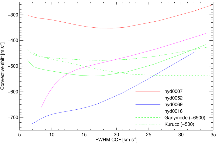
Figure 9: Convective shifts as a function of the FWHM of the cross-correlation peak. Four model spectra are plotted representative of various stellar types (see also Table 4): “hyd0007” K-dwarf, “hyd0052” G-dwarf, “hyd0069” F-dwarf, “hyd0016” red giant. The curves labelled “Kurucz” and “Ganymede” are for two solar spectra discussed in the text; their curves were arbitrarily shifted by -500 and -6500 m s^-1, respectively.

Finally, we would like to comment on the dependence of the convective shifts on spectral resolution. At first glance, one might think that the spectral resolution has no influence since commonly considered broadening mechanisms (instrumental broadening, micro-/macroturbulence, stellar rotation) broaden spectral lines symmetrically. However, one has to keep in mind that spectral lines are intrinsically asymmetric in stellar spectra, shifted differently depending on strength, and often blended. A change of spectral resolution alters their relative contributions contributions, and ultimately leads to a shift of the maximum of the cross-correlation function. Tonry & Davis (1979) conduct an analytic analysis of the cross-correlation technique and demonstrate a dependence of the measured RV on the width of the cross-correlation peak. Quantitatively, the effect depends on the particular circumstances. Figure 9 gives an illustration for the synthetic spectra and two solar spectra, namely those of Ganymede and from the atlas of Kurucz et al. (1984). It is apparent that in all cases there is a dependence, however it is weakest for the empirical atlases. Since the HARPS G2-mask was tailored after the solar spectrum one might conjecture that mismatches between line positions and strengths are smallest here, and that might lead to the weak dependence. Conversely, one might take this as a warning that significant mismatches between mask of observed spectrum might enhance the resolution dependence. In any case, we tried to carefully include the resolution effect in our estimates of the convective line shifts.

Appendix B Additional astrometric data

Table 5 provides some additional astrometric data for the cross-match between our final sample of 71 objects and the Gaia Archive (subsample of 65 objects). The table contains the distance from the cluster centre, $|\mathbf{r}-\mathbf{r}_{c}|$, and tangential components in the $\alpha$ and $\delta$ directions for the astrometric velocity vectors computed from G17 data. The tangential components are given by $V_{\alpha}=k\mu_{\alpha*}/\pi$ and $V_{\delta}=k\mu_{\delta}/\pi$, where $\mu_{\alpha*}=\mu_{\alpha}\cos{\delta}$ and $\mu_{\delta}$ are the proper motions given in mas yr^-1 and $k=4.74047$ km yr s^-1 is the factor that transforms from AU yr^-1 to km s^-1 (e.g., P98).

Table 5: Additional astrometric data.

#	HIP	$|\mathbf{r}-\mathbf{r}_{c}|$	$V_{\alpha}$	$V_{\delta}$		#	HIP	$|\mathbf{r}-\mathbf{r}_{c}|$	$V_{\alpha}$	$V_{\delta}$
		(pc)	(km s-1)	(km s-1)				(pc)	(km s-1)	(km s-1)
2	16529	12.08 $\pm$ 0.36	32.317 $\pm$ 0.354	-7.852 $\pm$ 0.086		43	19441	12.79 $\pm$ 0.39	26.129 $\pm$ 0.236	-0.920 $\pm$ 0.022
4	18327	8.51 $\pm$ 0.43	28.400 $\pm$ 0.266	-4.712 $\pm$ 0.046		44	19808	4.13 $\pm$ 1.14	25.346 $\pm$ 0.716	-4.523 $\pm$ 0.130
6	19148	4.28 $\pm$ 0.36	26.418 $\pm$ 0.293	-4.357 $\pm$ 0.050		45	19834	3.39 $\pm$ 0.33	25.865 $\pm$ 0.296	-4.141 $\pm$ 0.068
8	19781	3.79 $\pm$ 0.40	24.700 $\pm$ 0.331	-3.758 $\pm$ 0.052		46	19862	2.98 $\pm$ 0.68	25.799 $\pm$ 0.355	-4.966 $\pm$ 0.075
9	19796	5.90 $\pm$ 0.44	25.552 $\pm$ 0.275	-1.179 $\pm$ 0.016		47	20357	3.29 $\pm$ 0.57	24.164 $\pm$ 0.419	-4.436 $\pm$ 0.077
10	20146	1.74 $\pm$ 0.20	25.318 $\pm$ 0.313	-6.221 $\pm$ 0.078		48	20527	4.45 $\pm$ 0.55	23.575 $\pm$ 0.252	-3.862 $\pm$ 0.055
12	20480	4.77 $\pm$ 0.56	23.418 $\pm$ 0.293	-8.940 $\pm$ 0.113		51	20762	3.51 $\pm$ 0.24	23.845 $\pm$ 0.276	-3.765 $\pm$ 0.052
13	20492	2.11 $\pm$ 0.40	24.018 $\pm$ 0.274	-3.949 $\pm$ 0.051		52	20827	3.19 $\pm$ 0.49	23.375 $\pm$ 0.310	-4.478 $\pm$ 0.061
14	20557	5.41 $\pm$ 0.49	23.819 $\pm$ 0.328	-9.294 $\pm$ 0.128		53	21138	2.02 $\pm$ 0.44	22.646 $\pm$ 0.267	-5.224 $\pm$ 0.069
16	20826	4.34 $\pm$ 0.30	24.105 $\pm$ 0.274	-2.733 $\pm$ 0.032		54	21256	4.73 $\pm$ 0.36	22.336 $\pm$ 0.265	-9.538 $\pm$ 0.114
17	20850	2.86 $\pm$ 0.23	23.240 $\pm$ 0.265	-4.312 $\pm$ 0.052		55	21261	2.20 $\pm$ 0.53	22.578 $\pm$ 0.271	-7.616 $\pm$ 0.094
19	20949	13.27 $\pm$ 1.46	22.297 $\pm$ 0.514	-13.055 $\pm$ 0.301		56	21723	5.73 $\pm$ 0.39	20.787 $\pm$ 0.212	-3.275 $\pm$ 0.041
20	20978	2.13 $\pm$ 0.59	22.631 $\pm$ 0.258	-5.991 $\pm$ 0.070		57	22177	11.46 $\pm$ 0.27	19.972 $\pm$ 0.230	2.846 $\pm$ 0.044
21	21099	2.70 $\pm$ 0.19	23.244 $\pm$ 0.252	-8.575 $\pm$ 0.094		58	22253	10.21 $\pm$ 1.10	20.371 $\pm$ 0.333	-10.645 $\pm$ 0.174
22	21741	13.91 $\pm$ 1.04	21.206 $\pm$ 0.286	-10.789 $\pm$ 0.146		59	22271	8.46 $\pm$ 0.34	25.545 $\pm$ 0.357	-18.881 $\pm$ 0.263
23	22380	4.73 $\pm$ 0.22	18.475 $\pm$ 0.219	-8.153 $\pm$ 0.098		60	22654	6.42 $\pm$ 0.60	18.927 $\pm$ 0.216	-8.410 $\pm$ 0.100
24	22422	4.63 $\pm$ 0.34	19.695 $\pm$ 0.227	-5.790 $\pm$ 0.068		61	23312	13.71 $\pm$ 0.28	17.892 $\pm$ 0.223	2.455 $\pm$ 0.040
25	22566	15.10 $\pm$ 1.31	18.970 $\pm$ 0.323	-5.244 $\pm$ 0.090		62	13806	19.09 $\pm$ 0.35	36.991 $\pm$ 0.409	-8.925 $\pm$ 0.099
26	23069	10.45 $\pm$ 0.80	18.037 $\pm$ 0.251	-4.664 $\pm$ 0.068		63	13976	26.74 $\pm$ 0.15	36.693 $\pm$ 0.228	2.367 $\pm$ 0.016
27	23498	10.26 $\pm$ 0.75	16.694 $\pm$ 0.253	-4.544 $\pm$ 0.070		64	19786	4.71 $\pm$ 0.40	26.017 $\pm$ 0.340	-2.959 $\pm$ 0.041
28	23750	10.35 $\pm$ 0.86	16.268 $\pm$ 0.246	-7.864 $\pm$ 0.119		65	19793	6.00 $\pm$ 0.20	25.597 $\pm$ 0.290	-10.319 $\pm$ 0.117
29	24923	14.92 $\pm$ 0.73	13.646 $\pm$ 0.218	-3.556 $\pm$ 0.059		66	19934	6.41 $\pm$ 0.55	25.365 $\pm$ 0.320	-9.306 $\pm$ 0.118
31	15300	16.29 $\pm$ 0.33	33.491 $\pm$ 0.325	-8.819 $\pm$ 0.092		67	20082	2.54 $\pm$ 0.53	25.392 $\pm$ 0.258	-5.003 $\pm$ 0.060
32	15563	19.52 $\pm$ 0.25	33.905 $\pm$ 0.254	0.887 $\pm$ 0.017		68	20130	2.93 $\pm$ 0.21	24.607 $\pm$ 0.317	-7.964 $\pm$ 0.103
33	15720	19.47 $\pm$ 0.27	32.938 $\pm$ 0.271	-9.616 $\pm$ 0.082		70	20485	5.64 $\pm$ 0.69	24.442 $\pm$ 0.319	-5.176 $\pm$ 0.071
35	17766	14.22 $\pm$ 0.38	30.414 $\pm$ 0.280	1.127 $\pm$ 0.021		71	20563	1.26 $\pm$ 0.68	24.161 $\pm$ 0.455	-6.674 $\pm$ 0.127
36	18018	10.26 $\pm$ 0.42	29.452 $\pm$ 0.348	-9.288 $\pm$ 0.111		72	20577	1.66 $\pm$ 0.68	24.227 $\pm$ 0.283	-5.365 $\pm$ 0.063
37	18322	7.37 $\pm$ 0.45	28.505 $\pm$ 0.318	-2.228 $\pm$ 0.030		73	20741	1.21 $\pm$ 1.26	23.514 $\pm$ 0.505	-6.067 $\pm$ 0.130
38	18946	5.20 $\pm$ 0.19	27.761 $\pm$ 0.353	-7.594 $\pm$ 0.100		74	20815	1.33 $\pm$ 0.39	23.603 $\pm$ 0.436	-5.340 $\pm$ 0.099
39	19082	4.76 $\pm$ 0.25	27.399 $\pm$ 0.474	-7.328 $\pm$ 0.131		75	20899	0.63 $\pm$ 0.52	23.815 $\pm$ 0.306	-6.225 $\pm$ 0.080
40	19207	4.61 $\pm$ 0.57	26.401 $\pm$ 0.331	-4.203 $\pm$ 0.057		76	20951	1.47 $\pm$ 0.44	23.227 $\pm$ 0.255	-7.097 $\pm$ 0.080
41	19263	3.99 $\pm$ 0.43	26.433 $\pm$ 0.297	-5.390 $\pm$ 0.065		77	21317	2.02 $\pm$ 0.22	22.045 $\pm$ 0.245	-5.830 $\pm$ 0.066
42	19316	5.47 $\pm$ 0.52	25.932 $\pm$ 0.332	-2.361 $\pm$ 0.042

References

- Allende Prieto et al. (2009) Allende Prieto, C., Koesterke, L., Ramírez, I., Ludwig, H.-G., & Asplund, M. 2009, Memorie della Societa Astronomica Italiana, 80, 622
- Beckers (1977) Beckers, J. M. 1977, ApJ, 213, 900
- Böhm-Vitense et al. (2002) Böhm-Vitense, E., Robinson, R., Carpenter, K. et al. 2002, ApJ, 569, 941
- Bressan et al. (2012) Bressan, A., Marigo, P., Girardi, L. et al. 2012, MNRAS, 427, 127
- Chen et al. (2015) Chen, Y., Bressan, A., Girardi, L. 2015, MNRAS, 452, 1068
- Chen et al. (2014) Chen, Y., Girardi, L., Bressan, A. et al. 2014, MNRAS, 444, 2525
- Cochran et al. (2002) Cochran, W. D., Hatzes, A. P., & Paulson, D. B. 2002, AJ, 124, 565
- de Bruijne (2001) de Bruijne, J. H. J., Hoogerwerf, R., & de Zeeuw, P. T. 2001, A&A, 367, 111
- de Bruijne et al. (2002) de Bruijne, J. H. J., Reynolds, A. P., Perryman, M. A. C. et al. 2002, A&A, 381, L57
- Dumusque et al. (2012) Dumusque, X., Pepe, F., Lovis, C. et al. 2012, Nature, 491, 207
- Dutra-Ferreira et al. (2016) Dutra-Ferreira, L., Pasquini, L., Smiljanic, R. et al. 2016, A&A, 585, A75
- Dravins et al. (1999) Dravins, D., Lindegren, L., & Madsen, S. 1999, A&A, 348, 1040
- Einstein (1917) Einstein, A. 1917, SPAW, 142
- Forbes (1961) Forbes, E.G. 1961, The problem of the solar red shifts, University of St. Andrews (United Kingdom).
- Gaia Collaboration et al. (2017) Gaia Collaboration, van Leeuwen, F., Vallenari, A. et al. 2017, A&A, 601, A19 [G17]
- Geller et al. (2010) Geller, A. M., Mathieu, R. D., Braden, E. K. et al. 2010, AJ, 139, 1383
- Grevesse & Sauval (1998) Grevesse, N., & Sauval, A. J. 1998, SSRv, 85, 161
- Griffin (2012) Griffin, R. F. 2012, JApA, 33, 29
- Griffin et al. (1988) Griffin, R. F., Griffin, R. E. M., Gunn, J. E. et al. 1988, AJ, 96, 172
- Guenther et al. (2005) Guenther, E. W., Paulson, D. B., Cochran, W. D. et al. 2005, A&A, 442, 1031
- Hartkopf et al. (2001) Hartkopf, W. I., McAlister, H. A., & Mason, B. D. 2001, AJ, 122, 3480
- Haywood et al. (2016) Haywood, R. D., Collier Cameron, A., Unruh, Y. C. et al. 2016, MNRAS, 457, 3637
- Holberg (2010) Holberg, J. B. 2010, JHA, 41, 41
- Kurucz et al. (1984) Kurucz, R.L., Furenlid, I., Brault, J., and Testerman, L.: 1984, National Solar Observatory Atlas, Sunspot, New Mexico: National Solar Observatory, 1984
- Lanza et al. (2016) Lanza, A. F., Molaro, P., Monaco, L., & Haywood, R. D. 2016, A&A, 587, A103
- Lindegren & Dravins (2003) Lindegren, L., & Dravins, D. 2003 A&A, 401, 1185
- Lindegren et al. (2000) Lindegren, L., Madsen, S., & Dravins, D. 2000, A&A, 356, 1119
- Lo Curto et al. (2015) Lo Curto, G., Pepe, F., Avila, G. et al. 2015, Msngr, 162, 9
- Lovis et al. (2011) Lovis, C., Ségransan, D., Mayor, M. et al. 2011, A&A, 528, A112
- Ludwig, Freytag, & Steffen (1999) Ludwig H.-G., Freytag B., Steffen M., 1999, A&A, 346, 111
- Ludwig et al. (2017) Ludwig, H.-G., Koesterke, L., Allende Prieto, C., Bertran de Lis, S., Freytag, B., Caffau, E., 2017, in prep.
- Maderak et al. (2013) Maderak, R. M., Deliyannis, C. P., King, J. R. et al. 2013, AJ, 146, 143
- Madsen (2003) Madsen, S. 2003, A&A 401, 565
- Madsen et al. (2002) Madsen, S., Dravins, D., & Lindegren, L. 2002, A&A, 381, 446 [M02]
- Mason et al. (2009) Mason, B. D., Hartkopf, W. I., Gies, D. R. et al. 2009, AJ, 137, 3358
- Mayor et al. (2003) Mayor, M., Pepe, F., Queloz, D. et al. 2003, Msngr, 114, 20
- Molaro et al. (2016) Molaro, P., Lanza, A. F., Monaco, L. et al. 2016, MNRAS, 458, L54
- Pace & Pasquini (2004) Pace, G., & Pasquini, L. 2004, A&A, 426, 1021
- Pasquini et al. (2011) Pasquini, L., Melo, C., Chavero, C. et al. 2011, A&A, 526, A127
- Paulson et al. (2004) Paulson, D. B., Saar, S. H., Cochran, W. D. et al. 2004, AJ, 127, 1644
- Paulson et al. (2003) Paulson, D. B., Sneden, C., & Cochran, W. D. 2003, AJ, 125, 3185
- Pepe et al. (2002) Pepe F., Mayor M., Galland F., Naef D., Queloz D., Santos N. C., Udry S., Burnet M., 2002, A&A, 388, 632
- Perryman et al. (1998) Perryman, M. A. C., Brown, A. G. A., Lebreton, Y. et al. 1998, A&A, 331, 81 [P98]
- Piffl (2014) Piffl, T., Binney, J., McMillan, P. J. et al. 2014, MNRAS, 445, 3133
- Poretti (2001) Poretti, E. 2001, A&A, 371, 986
- Poretti et al. (2009) Poretti, E., Michel, E., Garrido, R. et al. 2009, A&A, 506, 85
- Quinn et al. (2014) Quinn, S. N., White, R. J., Latham, D. W. et al. 2014, ApJ, 787, 27
- Randich et al. (2000) Randich, S., Pasquini, L., & Pallavicini, R. 2000, A&A, 356, L25
- Reino et al. (2018) Reino, S., de Bruijne, J., Zari, E. et al. 2018, MNRAS, 477, 3197
- Saar & Donahue (1997) Saar, S. H., & Donahue, R. A. 1997, ApJ, 485, 319
- Tang et al. (2014) Tang, J., Bressan, A., Rosenfield, P. 2014, MNRAS, 445, 4287
- Tonry & Davis (1979) Tonry J., Davis M., 1979, AJ, 84, 1511
- van Leeuwen (2007) van Leeuwen, F. 2007, A&A, 474, 653
- van Leeuwen (2009) van Leeuwen, F. 2009, A&A, 497, 209
- Vereshchagin & Chupina (2013) Vereshchagin, S.V., & Chupina, N. V. 2013, AN, 334, 892