MATMPC - A MATLAB Based Toolbox for Real-time Nonlinear Model Predictive Control

Abstract

In this paper we introduce MATMPC, an open source software built in MATLAB for nonlinear model predictive control (NMPC). It is designed to facilitate modelling, controller design and simulation for a wide class of NMPC applications. MATMPC has a number of algorithmic modules, including automatic differentiation, direct multiple shooting, condensing, linear quadratic program (QP) solver and globalization. It also supports a unique Curvature-like Measure of Nonlinearity (CMoN) MPC algorithm. MATMPC has been designed to provide state-of-the-art performance while making the prototyping easy, also with limited programming knowledge. This is achieved by writing each module directly in MATLAB API for C. As a result, MATMPC modules can be compiled into MEX functions with performance comparable to plain C/C++ solvers. MATMPC has been successfully used in operating systems including WINDOWS, LINUX AND OS X. Selected examples are shown to highlight the effectiveness of MATMPC.

I introduction

In recent years, together with an increase of computational power, the number of applications of linear and nonlinear MPC for fast-dynamics systems has considerably grown. While several linear MPC tools (both commercial [1, 2] and open-source [3],) are mature and available, the number of software for nonlinear MPC (NMPC) is rather limited [4].

I-A NMPC software packages

Existing NMPC software packages can be categorized into two main classes. The first one is characterized by software written in MATLAB and aims at algorithm development, tuning, and offline simulation, as MATLAB functions are flexible to edit and easy to understand. Popular software includes GPOPS [5], ICLOCS2 [6] and CasADi [7]. While they are very flexible and powerful for algorithm prototyping and debugging, the computational efficiency is lost as MATLAB is not designed for computational efficiency. Therefore, it is difficult to know how efficient the NMPC algorithm is for practical applications without actually implementing it in embedded hardware.

Another class of NMPC software focus on embedded hardware and fast deployment. There are two main structures of such software, one based on automatic code generation and the other one employing a modular structure. The former generates a tailored piece of code of NMPC algorithm for a specific application. Software with this structure includes GMRES [8], ACADO [9], VIATOC [10] and Forces Pro [11]. The advantage of such implementations is that the code generated is compact, self-contained and is very likely efficient and hardware compatible [12]. However, it lacks flexibility and maintainability since code generation is a “black box” to users. While code generation software is efficient and can be deployed instantly, it is not suitable for algorithm prototyping and debugging. The latter has a modular structure, where independent algorithmic modules are implemented. Among this class, ACADOS is a C library that is computational efficient as well as flexible [12]. CT is a C++ library of a class of algorithms for robotic applications [13]. It has a number of modules including MPC and has been deployed for many real-time NMPC applications. Although efficient and useful, such software requires a decent knowledge of low-level programming languages like C/C++. In addition, additional efforts are needed to build such software at different operating systems, in different hardware structures or high level interfaces such as MATLAB and Python.

I-B Features of MATMPC

MATMPC aims at filling the gap between the two aforementioned classes of MPC software, by taking advantages from both sides. First, MATMPC is mainly written in MATLAB language and can be easily embedded in SIMULINK applications, making algorithm development and NMPC simulation extremely easy and flexible. Second, MATMPC has a modular structure and its time critical modules are written in MATLAB application program interface (API) for C. These modules are compiled into MEX functions which stand for MATLAB executable. As a result, NMPC simulation using MATMPC can achieve a competitive runtime performance against other C/C++ software. In fact, MATMPC is not a library that needs to be compiled at a given operating system before its usage, but a collection of NMPC routines that only relies on MATLAB without external library dependencies at compilation time. Each module can be replaced by another one in MATMPC or by one written by users, since modules are independent from each other.

MATMPC supports a variety of algorithms that can be easily replaced for different applications. It exploits direct multiple shooting to discretize the optimal control problem (OCP) into Nonlinear Programming problem (NLP) based on dynamic models governed by explicit or implicit ordinary differential equations. Efficient numerical integrators, e.g. explicit and implicit Runge-Kutta integrators, are implemented to approximate continuous trajectory of systems. MATMPC uses sequential quadratic programming (SQP) methods to solve the NLP. Stable condensing algorithms are employed to convert the sparse quadratic program (QP) into (partial) dense QP. A number of QP solvers are embedded, that can be selected to best fit the specific application at hand. A line search globalization algorithm is provided for searching local minimum of NLP, giving more flexibility to trade off solution accuracy and runtime performance.

In MATMPC, a Curvature-like Measure of Nonlinearity (CMoN) SQP algorithm [14] is implemented. This algorithm allows to update only part of sensitivities of system dynamics between two consecutive iterations and sampling instants. The number of updated sensitivities are monitored by CMoN and automatically determined on-line, depending on how nonlinear the system is. Its control and numerical performance, including computational efficiency, robustness and convergence, is demonstrated in [14].

MATMPC is open source available under GPL v3 at https://github.com/chenyutao36/MATMPC.

I-C Paper structure

This paper is structured as follows. Section II gives an introduction of algorithms employed in MATMPC. In Section III, details of modules and overall features of MATMPC are given. A nontrivial simulation example using MATMPC is described in Section IV, followed by the conclusions in Section V.

II Algorithm basics

In MATMPC, a NLP is formulated by applying direct multiple shooting [15] to an OCP over the prediction horizon $T=[t_{0},t_{f}]$, which is divided into $N$ shooting intervals $[t_{0},t_{1},\ldots,t_{N}]$, as follows:

$$\min_{x_{k},u_{k}}\, \sum_{k=0}^{N-1}\frac{1}{2}\lVert h_{k}(x_{k},u_{k})\rVert_{W}^{2}+\frac{1}{2}\lVert h_{N}(x_{N})\rVert_{W_{N}}^{2}$$ (1a)

$$s.t.\, 0=x_{0}-\hat{x}_{0},$$ (1b)

$$0=x_{k+1}-\phi_{k}(x_{k},u_{k}),\,k=0,1,\ldots,N-1,$$ (1c)

$$\underline{r}_{k}\leq r_{k}(x_{k},u_{k})\leq\overline{r}_{k},\,k=0,1,\ldots,N-1,$$ (1d)

$$\underline{r}_{N}\leq r_{N}(x_{N})\leq\overline{r}_{N},$$ (1e)

where $\hat{x}_{0}$ is the measurement of the current state. System states $x_{k}\in\mathbb{R}^{n_{x}}$ are defined at the discrete time point $t_{k}$ for $k=0,\ldots,N$ and the control inputs $u_{k}\in\mathbb{R}^{n_{u}}$ for $k=0,\ldots,N-1$ are piece-wise constant. Here, (1d) is defined by $r(x_{k},u_{k}):\mathbb{R}^{n_{x}}\times\mathbb{R}^{n_{u}}\rightarrow\mathbb{R}^{n_{r}}$ and $r(x_{N}):\mathbb{R}^{n_{x}}\rightarrow\mathbb{R}^{n_{l}}$ with lower and upper bound $\underline{r}_{k},\overline{r}_{k}$. Equation (1c) refers to the continuity constraint where $\phi_{k}(x_{k},u_{k})$ is a numerical integration operator that solves the following initial value problem (IVP) and returns the solution at $t_{k+1}$.

$$0=f(\dot{x}(t),x(t),u(t),t),\quad x(0)=x_{k}.$$ (2)

II-A Sequential Quadratic Programming

We introduce the compact notation

$$\mathbf{x}=\left[x_{0}^{\top},x_{1}^{\top},\dots,x_{N}^{\top}\right]^{\top},$$ (3)

$$\mathbf{u}=\left[u_{0}^{\top},u_{1}^{\top},\dots,u_{N-1}^{\top}\right]^{\top}$$

for the discrete state and control variables. Problem (1) is solved using SQP method, where at iteration $i$, a QP problem is formulated as

$$\begin{split}\min_{\Delta\mathbf{x},\Delta\mathbf{u}}\quad&\sum_{k=0}^{N-1}(\frac{1}{2}\begin{bmatrix}\Delta x_{k}\\ \Delta u_{k}\end{bmatrix}^{\top}H^{i}_{k}\begin{bmatrix}\Delta x_{k}\\ \Delta u_{k}\end{bmatrix}+g_{k}^{i^{\top}}\begin{bmatrix}\Delta x_{k}\\ \Delta u_{k}\end{bmatrix})\\ &+\frac{1}{2}\Delta x_{N}^{\top}H^{i}_{N}\Delta x_{N}+g_{N}^{i^{\top}}\Delta x_{N}\\ s.t.\quad&\Delta x_{0}=\hat{x}_{0}-x_{0},\\ &\Delta x_{k+1}=A_{k}^{i}\Delta x_{k}+B_{k}^{i}\Delta u_{k}+d_{k}^{i},\\ &\underline{c}_{k}^{i}\leq C_{k}^{i}\Delta x_{k}+D_{k}^{i}\Delta u_{k}\leq\overline{c}_{k}^{i},\\ &\underline{c}_{N}^{i}\leq C_{N}^{i}\Delta x_{N}\leq\overline{c}_{N}^{i},\end{split}$$ (4)

where $\Delta\mathbf{x}=\mathbf{x}-\mathbf{x}^{i},\Delta\mathbf{u}=\mathbf{u}-\mathbf{u}^{i}$ and for $k=0,1,\ldots,N-1$

$$\begin{split}&H_{k}^{i}=\frac{\partial h_{k}^{i}}{\partial(x_{k},u_{k})}^{\top}\frac{\partial h_{k}^{i}}{\partial(x_{k},u_{k})},\quad g_{k}^{i}=\frac{\partial\lVert h_{k}^{i}\rVert_{W}^{2}}{\partial(x_{k},u_{k})},\\ &A_{k}^{i}=\frac{\partial\phi_{k}}{\partial x_{k}}(x_{k}^{i},u_{k}^{i}),\quad B_{k}^{i}=\frac{\partial\phi_{k}}{\partial u_{k}}(x_{k}^{i},u_{k}^{i}),\\ &C_{k}^{i}=\frac{\partial r_{k}}{\partial x_{k}}(x_{k}^{i},u_{k}^{i}),\quad D_{k}^{i}=\frac{\partial r_{k}}{\partial u_{k}}(x_{k}^{i},u_{k}^{i}),\\ &\overline{c}_{k}^{i}=\overline{r}_{k}-r_{k}(x_{k}^{i},u_{k}^{i}),\quad\underline{c}_{k}^{i}=\underline{r}_{k}-r_{k}(x_{k}^{i},u_{k}^{i}),\\ &d_{k}^{i}=\phi(x_{k}^{i},u_{k}^{i})-x_{k+1}^{i}.\end{split}$$ (5)

Here we use Gauss-Newton Hessian approximation to compute $H_{k}^{i}$ as it is a good approximate of the exact Hessian for the least square cost function in (1) and it is always positive semi-definite. The QP problem (4) has a special structure and can be solved by structure exploiting or sparse solvers, such as HPIPM [16], OSQP [17], and Ipopt [18].

An alternative is to first condense problem (4) [19] and obtain a dense QP problem as follows:

$$\min_{\Delta\mathbf{u}} \frac{1}{2}{\Delta\mathbf{u}}^{\top}H_{c}{\Delta\mathbf{u}}+g_{c}^{\top}\Delta\mathbf{u}$$ (6)

$$s.t. \underline{c}_{c}\leq C_{c}\Delta\mathbf{u}\leq\overline{c}_{c},$$

Problem (6) can be solved by dense QP solvers like qpOASES [20]. It is also possible to use partial condensing [21] to obtain a smaller but still sparse QP problem. Computation efficiency improvement using partial condensing has been reported in [22, 23].

The solution of (4) is used to update the solution of (1) by

$$\mathbf{x}^{i+1}=\mathbf{x}^{i}+\alpha^{i}\Delta\mathbf{x}^{i},\,\mathbf{u}^{i+1}=\mathbf{u}^{i}+\alpha^{i}\Delta\mathbf{u}^{i},$$ (7)

where $\alpha^{i}$ is the step length determined by globalization strategies. A practical line search SQP algorithm employing $\ell_{1}$ merit function [24] is employed in MATMPC. The merit function is defined as

$$m(\mathbf{w};\mu)=l(\mathbf{w})+\mu\lVert e(\mathbf{w})\rVert_{1}$$ (8)

where $\mathbf{w}=[\mathbf{x}^{\top},\mathbf{u}^{\top}]^{\top}$, $l(\mathbf{w})$ is the objective function of (1), $e(\mathbf{w})$ contains all constraints in (1) with slack variables for inequality constraints and $\mu$ the penalty parameter. The step $\alpha^{i}\Delta\mathbf{w}^{i}$ is accepted if

$$m(\mathbf{w}^{i}+\alpha^{i}\Delta\mathbf{w}^{i};\mu^{i})\leq m(\mathbf{w}^{i};\mu^{i})+\eta\alpha^{i}\mathcal{D}(m(\mathbf{w}^{i};\mu^{i});\Delta\mathbf{w}^{i})$$ (9)

where $\mathcal{D}(m(\mathbf{w}^{i};\mu^{i});\Delta\mathbf{w}^{i})$ is the directional derivative of $m$ in the direction of $\Delta\mathbf{w}^{i}$. We adopt Algorithm 18.3 ([24], p. 545) to choose $\mu^{i}$ and compute $\alpha^{i}$ at each iteration. An alternative is to compute a suboptimal solution by terminating the SQP iteration early before convergence is achieved. For many applications, it is sufficient to use only one iteration with a full Newton step $\alpha=1$. Such strategy is the so-called Real-Time Iteration (RTI) scheme [25] and is supported in MATMPC.

TABLE I: Available options in MATMPC

Hessian Approximation	Gauss-Newton
Integrator	Explicit Runge Kutta 4 (CasADi code generation)	Explicit Runge Kutta 4	Implicit Runge-Kutta (Gauss-Legendre)
Condensing	non	full	partial
QP solver	qpOASES	MATLAB quadprog	Ipopt
	OSQP	HPIPM
Globalization	$\ell_{1}$ merit function line search		Real-Time Iteration
Additional features	CMoN-SQP		input MB

II-B Curvature-like measure of nonlinearity SQP

In MATMPC, the CMoN-SQP algorithm [14] is implemented to adaptively update system sensitivities on-line. The updating rule is given by

$$\nabla\phi_{k}^{i}=\left\{\begin{array}[]{l}\nabla\phi_{k}^{i-1},\>\text{if}\>\>\kappa_{k}^{i}\leq\eta^{i}_{pri}\,\&\,\tilde{\kappa}_{k}^{i}\leq\eta_{dual}^{i},\\ \text{eval}(\nabla\phi_{k}^{i}),\,\text{otherwise}\end{array}\right.$$ (12)

where $\nabla\phi_{k}=[A_{k},B_{k}],k=0,\ldots,N-1$ is the sensitivity matrix, $(\eta^{i}_{pri},\eta_{dual}^{i})$ the CMoN threshold. The CMoN value is defined as

$$\kappa_{k}^{i}\coloneqq\frac{\lVert\phi_{k}^{i}-\phi_{k}^{i-1}-\nabla\phi_{k}^{i-1}q_{k}^{i-1}\rVert}{\lVert\nabla\phi_{k}^{i-1}q_{k}^{i-1}\rVert},$$ (13)

$$\tilde{\kappa}_{k}^{i}\coloneqq\frac{\lVert\Delta\lambda^{i-1^{\top}}_{k+1}(\nabla\phi_{k}^{i}-\nabla\phi_{k}^{i-1})\rVert}{\lVert\Delta\lambda^{i-1^{\top}}_{k+1}\nabla\phi_{k}^{i-1}\rVert},$$ (14)

where $q_{k}^{i-1}=[x_{k}^{i}-x_{k}^{i-1},u_{k}^{i}-u_{k}^{i-1}]^{\top},\Delta\lambda_{k}^{i-1}=\lambda_{k}^{i}-\lambda_{k}^{i-1}$ are the increments on primal and dual variables between two iterations, respectively. Here, the CMoN value is an indicator of local nonlinearity of system and the updating rule (12) ensures that only sufficiently nonlinear sensitivities are updated, possibly reducing computational burden.

CMoN-SQP only requires two user defined parameters $(\epsilon^{abs},\epsilon^{rel})$ that are absolute and relative tolerances of the accuracy of solution of (4). In [14], it is proved that the threshold $(\eta^{i}_{pri},\eta_{dual}^{i})$ is a function of $(\epsilon^{abs},\epsilon^{rel})$. Hence, by defining the tolerance off-line, the CMoN threshold is automatically updated and the number of updated sensitivities is determined by CMoN-SQP on-line. In addition, CMoN-SQP supports the adoption of the RTI scheme by updating partial sensitivities between two sampling instants.

III Structure of MATMPC

III-A Overview

MATMPC is a collection of MATLAB functions, including standard and MEX ones. MATMPC is an open source software (GPL v3) written in MATLAB and MATLAB C API. It consists of a number of algorithmic modules which can be easily replaced or extended. MATMPC aims at fast and flexible algorithm prototyping and competitive run-time performance.

III-B Modules of MATMPC

MATMPC consists of two main functions, namely the model_generation and the simulation. The model_generation function takes user-defined dynamic models and generates C codes of model analytic functions and their derivatives, by employing automatic differentiation (AD) in CasADi [7]. Note that MATMPC only generates codes from model dynamics, taking model and optimization parameters as parameters that can be altered on-line. On the other hand, other NMPC code generation tools generate ready to use codes that include the entire NMPC algorithm. Therefore, users can change model or optimization parameters on-line without repeatedly running model_generation function in MATMPC.

The simulation function is for running closed-loop NMPC simulations in MATLAB. It starts from initializing controller options, data and memories defined in MATLAB struct format. Available options in MATMPC are given in Table I. The NMPC controller in MATMPC is a MATLAB function that calls a number of modules. They include qp_generation for performing multiple shooting, condensing for performing (partial) condensing routines, qp_solve for calling QP solvers, solution_info for computing optimal solution information such as constraint residual and Karush$-$Kuhn$-$Tucker (KKT) value, and line_search for performing globalization. These modules are MEX functions which share the same data and memory structs created at initialization, without the need to allocate any memory on-line. In addition, as data memory structs are globally accessible in MATLAB, it is possible to pause simulation and inspect intermediate data when debugging, just like running standard MATLAB functions.

In MATMPC, there are two sources of external dependencies. The first is CasADi [7] for performing AD and generating C codes of model functions and derivatives. CasADi is an open source software and has pre-compiled MATLAB binaries ready to use. The second source is from QP solvers, that are carefully selected ones for NMPC applications from the open source software pool. MATMPC provides pre-compiled MATLAB binaries and interfaces for all QP solvers listed in Table I. While qpOASES is a dense QP solver, all the others are sparse or structure exploiting solvers. They can be called directly after multiple shooting, or after a partial condensing step that returns a smaller but also sparse QP problem. Note that these two external dependencies do not require additional compiling or installing processes.

III-C Features

MATMPC has two main advantages over other NMPC software. First, the algorithm modules are written in MATLAB C API hence they can be compiled into MEX functions by using MinGW or GCC. Since these MEX functions rely on MATLAB only and not on a given operating system, MATMPC can work in WINDOWS, LINUX and OS X without any code modifications. MATMPC also employs MATLAB built-in linear algebra routines which are BLAS and LAPACK libraries from Intel MKL [26]. As a result, the compilation of MEX functions does not depend on any external header files or libraries. MATMPC is not a library but a collection of NMPC routines, each of which can be easily replaced or extended according to user needs. Second, there is no requirement on programming knowledge other than MATLAB. Users can try different combination of algorithm modules, tuning parameters and simulation modes without writing any C codes. It is also easy to replace existing modules by user defined MATLAB or MEX functions, since in MATLAB, there is no memory nor format requirement for these functions.

III-D Examples

MATMPC provides several examples to illustrate its usage. The list of examples is

1. Inverted Pendulum [27]

2. Chain of Masses (linear [28] and nonlinear [14])

3. Hexacopter and tethered quadropter

These examples range from classical problems to state-of-art NMPC applications.

IV Co-simulation using MATMPC

We present an example of using MATMPC in a co-simulation of an automotive application: the software has been used to develop an MPC-based controller for an autonomous vehicle. The vehicle simulation model comes from a commercial simulation environment and MATMPC computes the optimal steering, throttle, and brake controls in order to follow a given trajectory.

IV-A Control Model

The internal model used by the controller is a four-wheel vehicle, with longitudinal forces based on a linear tire model and lateral forces based on decoupled Paceijka’s magic formula [29]. We consider the vehicle model as

$$\dot{\xi}=f(\xi(t),u(t)),$$ (15)

where $\xi(t)\in\mathbb{R}^{n_{x}}$ is the state of the vehicle and $u(t)\in\mathbb{R}^{n_{u}}$ is the input. The dynamics $f$ is derived using the equation of motion of the vehicle’s center of mass (CG) [30], i.e.

$$\ddot{x} =\dot{y}\dot{\psi}+\frac{1}{m}\left(\sum_{i,j}F_{x_{i,j}}-F_{x}^{d}\right),$$ (16)

$$\ddot{y} =-\dot{x}\dot{\psi}+\frac{1}{m}\left(\sum_{i,j}F_{y_{i,j}}\right),$$

$$\ddot{\psi} =\frac{1}{I_{z}}\Bigg{[}a\left(\sum_{j}F_{y_{f,j}}\right)-b\left(\sum_{j}F_{y_{r,j}}\right)$$

$$+c\left(\sum_{i}F_{x_{i,r}}-\sum_{i}F_{x_{i,l}}\right)\Bigg{]}$$

where $x,y,\psi$ are longitudinal, lateral positions and yaw angle. Subscripts $i\in\{f,r\}$ indicates front or rear wheels, $j\in\{l,r\}$ left or right wheels and $a,b,c$ are the dimensional parameters (respectively front wheels - CG longitudinal distance, rear wheels - CG longitudinal distance and wheels CG lateral distance). $F_{\{x,y\}_{\{i,j\}}}$ are the lateral and longitudinal forces on the wheels in the car reference frame and $F_{x}^{d}$ is the longitudinal drag force, detailed in Fig. 1. Finally, the slip angle of the vehicle is defined as $\beta=atan\left(\frac{\dot{y}}{\dot{x}}\right)$.

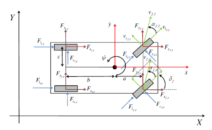
Figure 1: Forces, velocities and angles defined in the vehicle’s internal model

In order to eliminate the dependency on the velocity in the reference given to the MPC, the dynamics has been reformulated in spatial coordinates w.r.t. $s$, the arc length along the track. The tracking errors $e_{\psi}=\psi-\psi_{ref}$ and $e_{y}=\lVert[X,Y]^{\top}-[X_{ref},Y_{ref}]^{\top}\rVert_{2}$ are treated as additional system states. The resulting state vector is $\xi=[\dot{x},\dot{y},\dot{\psi},\dot{e}_{\psi},\dot{e}_{y}]^{T}$ and its derivative w.r.t $s$ is obtained using the chain rule [31] as

$$\xi^{\prime}=\frac{d\xi}{ds}=\frac{d\xi}{dt}\frac{dt}{ds}=\frac{d\xi}{dt}\frac{1}{\dot{s}}=\frac{\dot{\xi}}{\dot{s}},$$ (17)

where $\dot{s}=\frac{1}{1-k\ e_{y}}\left(\dot{x}\ cos(e_{\psi})-\dot{y}\ sin(e_{\psi}\right)$. The inputs of the system are $u=[\delta_{f},\gamma]^{\top}$, where $\delta_{f}$ is the steering wheel angle and $\gamma$ is the normalized throttle/braking action.

IV-B Co-simulation environment

The co-simulation relied on VI-CarRealTime (VI-CRT), a simulation software specifically designed to reproduce vehicles’ behaviour for high performance driving in real time [32]. Its simulation model has 14 degree of freedoms, 6 for the chassis and 2 for each wheel and it includes comprehensive dynamics of tire, chassis, suspensions, brakes, engine and transmission. The co-simulation is performed in Simulink, connecting a VI-CRT simulation block with MATMPC controller, as shown in Fig. 2. In particular, VI-CRT is used to simulate at $f_{s}^{sim}=1000$ Hz the dynamics of the vehicle while the control action is updated by MATMPC at $f_{s}^{ctrl}=50$ Hz. The simulations have been made on a PC in WINDOWS 10, with Intel(R) Core(TM) i7-7700HQ CPU running at 2.80GHz.

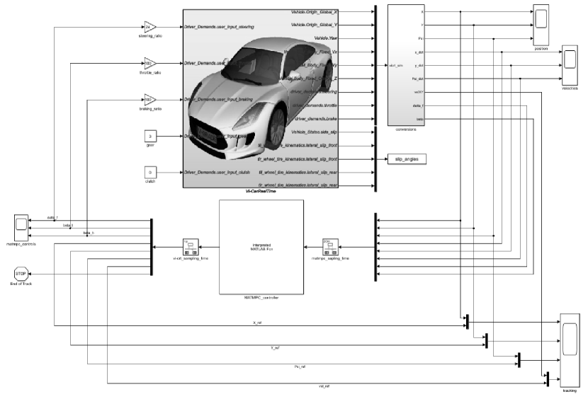
Figure 2: Simulink co-simulation block diagram

IV-C Controller setup

The optimization problem has the form of (1) where the cost functions are defined as

$$h_{k}(x_{k},u_{k})=[v-v_{ref},e_{y},\dot{e}_{y},e_{\psi}+\beta,\dot{e}_{\psi},\dot{\delta_{f}},\dot{\gamma}]^{\top},$$ (18)

$$h_{N}(x_{k},u_{k})=[v-v_{ref},e_{y},\dot{e}_{y},e_{\psi}+\beta,\dot{e}_{\psi}]^{\top}$$

where $v=\sqrt{\dot{x}^{2}+\dot{y}^{2}}$ is vehicle’s velocity. The weights are given as

$$W=\text{diag}([10^{0},10^{2},10^{-2},10^{2},10^{-2},10^{1},10^{-1}]),$$ (19)

$$W_{N}=\text{diag}([10^{0},10^{2},10^{-2},10^{2},10^{1}]).$$

The constraint functions are defined as

$$r_{k}=[e_{\psi},e_{y},\delta_{f},\gamma,\dot{\delta_{f}},\dot{\gamma}]^{\top},$$ (20)

$$r_{N}=[e_{\psi},e_{y},\delta_{f},\gamma]^{\top}$$

with bounds

$$\underline{r}_{k}=[-\frac{\pi}{2},-5,-\frac{\pi}{6},-1,-1,-5]^{\top},$$ (21)

$$\overline{r}_{k}=[+\frac{\pi}{2},+5,+\frac{\pi}{6},+1,+1,+5]^{\top},$$

$$\underline{r}_{N}=[-\frac{\pi}{2},-5,-\frac{\pi}{6},-1]^{\top},$$

$$\overline{r}_{N}=[+\frac{\pi}{2},+5,+\frac{\pi}{6},+1]^{\top}.$$

The options used in MATMPC for the simulation are summarized in Table II. For the integrator, we employ two integration steps per shooting interval of length $T_{s}=2$ meters. A total number of $N=75$ shooting intervals are used, enabling a prediction length of $150$ meters on track.

TABLE II: MATMPC options used for the co-simulation

	Selected module
Integrator	Explicit Runge Kutta 4
Condensing	Non
QP Solver	HPIPM
Globalization	Real-Time Iteration

IV-D Results using standard NMPC

The simulations have been performed on VI-Track (see Fig. 3), a virtual circuit available with a standard installation of VI-CRT. The reference velocity profile is obtained minimizing the lap-time by means of VI-maxperf, a tool embedded in VI-CRT that allows to compute minimum lap time simulation. The velocity profile and reference is shown in Fig. 4. The MPC controller has a considerably good tracking performance while satisfying vehicles dynamics and constraints. Indeed, the MATMPC controller has been compared with the commercial controller developed by VI-Grade that aims at driving the vehicle at the maximum performance. The MATMPC controller is able to complete the track with a smaller lap time ($T_{track}^{VI-Grade}=59.4s$ vs $T_{track}^{MPC}=59.1s$), showing superior performance of MPC on this application. The computational time for the controller is $T_{solver}^{mean}=3.0$ ms and $T_{solver}^{max}=10.5$ ms, showing real-time capability of MATMPC despite running in MATLAB environment.

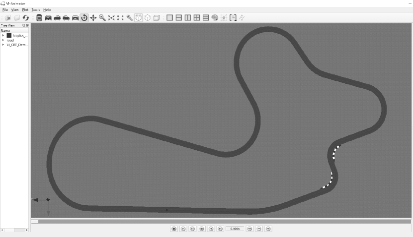
Figure 3: Simulation track in VI-CRT

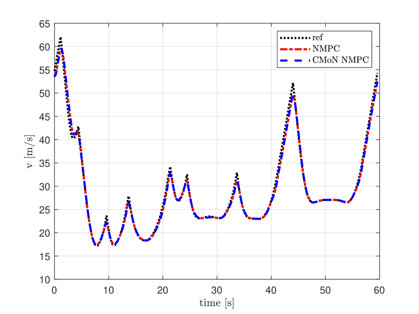
Figure 4: Simulation velocity profile and reference

IV-E Results using CMoN NMPC

We also present results using the CMoN scheme, introduced in (12) from [14]. We use the controller configurations described in Section IV-D, except for the activation of the CMoN strategy. The absolute and relative tolerance on primal and dual solutions of QP (4) are $(\epsilon^{abs},\epsilon^{rel})=(10^{-1},10^{-1})$. As can be seen in Fig. 4, the tracking performance of the CMoN scheme is indistinguishable from that of the standard NMPC. However, Fig. 5 shows that the percentage of exactly updated sensitivities at each sample is at most $80\%$ and in average less than $20\%$. It demonstrates the effectiveness of the CMoN scheme for a non-trivial application.

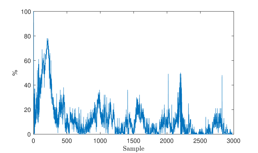
Figure 5: Percentage of exactly updated sensitivities at each sample during closed-loop simulation using CMoN-RTI scheme

V Conclusion

In this paper, we introduce MATMPC, a NMPC software based on MATLAB. We present briefly the NMPC algorithm used in MATMPC, and a detailed description of the structure and features of MATMPC. Through a non-trivial vehicle control application, the effectiveness and efficiency of MATMPC is demonstrated.

References

- [1] S. J. Qin and T. A. Badgwell, “A survey of industrial model predictive control technology,” Control engineering practice, vol. 11, no. 7, pp. 733–764, 2003.
- [2] A. Bemporad, M. Morari, and N. L. Ricker, “Model predictive control toolbox 3 user’s guide,” The mathworks, 2010.
- [3] J. Lofberg, “Yalmip: A toolbox for modeling and optimization in matlab,” in Computer Aided Control Systems Design, 2004 IEEE International Symposium on. IEEE, 2004, pp. 284–289.
- [4] S. J. Qin and T. A. Badgwell, “An overview of nonlinear model predictive control applications,” Nonlinear model predictive control, pp. 369–392, 2000.
- [5] M. A. Patterson and A. V. Rao, “Gpops-ii: A matlab software for solving multiple-phase optimal control problems using hp-adaptive gaussian quadrature collocation methods and sparse nonlinear programming,” ACM Transactions on Mathematical Software (TOMS), vol. 41, no. 1, p. 1, 2014.
- [6] Y. Nie, O. Faqire, and E. C. Kerrigan, “Iclocs2: Solve your optimal control problems with less pain,” in IFAC Conference on Nonlinear Model Predictive Control. IFAC, 2018, pp. 00–00.
- [7] J. A. Andersson, J. Gillis, G. Horn, J. B. Rawlings, and M. Diehl, “Casadi: a software framework for nonlinear optimization and optimal control,” Mathematical Programming Computation, pp. 1–36, 2018.
- [8] T. Ohtsuka and A. Kodama, “Automatic code generation system for nonlinear receding horizon control,” Transactions of the Society of Instrument and Control Engineers, vol. 38, no. 7, pp. 617–623, 2002.
- [9] B. Houska, H. J. Ferreau, and M. Diehl, “An auto-generated real-time iteration algorithm for nonlinear mpc in the microsecond range,” Automatica, vol. 47, no. 10, pp. 2279–2285, 2011.
- [10] J. Kalmari, J. Backman, and A. Visala, “A toolkit for nonlinear model predictive control using gradient projection and code generation,” Control Engineering Practice, vol. 39, pp. 56–66, 2015.
- [11] A. Zanelli, A. Domahidi, J. Jerez, and M. Morari, “Forces nlp: an efficient implementation of interior-point methods for multistage nonlinear nonconvex programs,” International Journal of Control, pp. 1–17, 2017.
- [12] R. Verschueren, G. Frison, D. Kouzoupis, N. van Duijkeren, A. Zanelli, R. Quirynen, and M. Diehl, “Towards a modular software package for embedded optimization,” in IFAC Conference on Nonlinear Model Predictive Control. IFAC, 2018, pp. 00–00.
- [13] M. Giftthaler, M. Neunert, M. Stäuble, and J. Buchli, “The control toolbox—an open-source c++ library for robotics, optimal and model predictive control,” in Simulation, Modeling, and Programming for Autonomous Robots (SIMPAR), 2018 IEEE International Conference on. IEEE, 2018, pp. 123–129.
- [14] Y. Chen, M. Bruschetta, D. Cuccato, and A. Beghi, “An adaptive partial sensitivity updating scheme for fast nonlinear model predictive control,” IEEE Transactions on Automatic Control, 2018.
- [15] H. G. Bock and K.-J. Plitt, “A multiple shooting algorithm for direct solution of optimal control problems,” in Proceedings of the IFAC World Congress, 1984.
- [16] “Hpipm,” https://github.com/giaf/hpipm, 2017.
- [17] B. Stellato, G. Banjac, P. Goulart, A. Bemporad, and S. Boyd, “OSQP: An operator splitting solver for quadratic programs,” ArXiv e-prints, Nov. 2017.
- [18] A. Wächter and L. T. Biegler, “On the implementation of an interior-point filter line-search algorithm for large-scale nonlinear programming,” Mathematical programming, vol. 106, no. 1, pp. 25–57, 2006.
- [19] J. Andersson, “A General-Purpose Software Framework for Dynamic Optimization,” PhD thesis, Arenberg Doctoral School, KU Leuven, Department of Electrical Engineering (ESAT/SCD) and Optimization in Engineering Center, Kasteelpark Arenberg 10, 3001-Heverlee, Belgium, October 2013.
- [20] H. J. Ferreau, C. Kirches, A. Potschka, H. G. Bock, and M. Diehl, “qpoases: A parametric active-set algorithm for quadratic programming,” Mathematical Programming Computation, vol. 6, no. 4, pp. 327–363, 2014.
- [21] C. Yutao, “Algorithms and applications for nonlinear model predictive control with long prediction horizon,” Ph.D. dissertation, University of Padova, 2018.
- [22] G. Frison, D. Kouzoupis, J. B. Jørgensen, and M. Diehl, “An efficient implementation of partial condensing for nonlinear model predictive control,” in Decision and Control (CDC), 2016 IEEE 55th Conference on. IEEE, 2016, pp. 4457–4462.
- [23] Y. Chen, G. Frison, N. van Duijkeren, M. Bruschetta, A. Beghi, and M. Diehl, “Efficient partial condensing algorithms for nonlinear model predictive control with partial sensitivity update,” in IFAC Conference on Nonlinear Model Predictive Control. IFAC, 2018, pp. 00–00.
- [24] J. Nocedal and S. Wright, Numerical optimization. Springer Science & Business Media, 2006.
- [25] M. Diehl, H. G. Bock, J. P. Schlöder, R. Findeisen, Z. Nagy, and F. Allgöwer, “Real-time optimization and nonlinear model predictive control of processes governed by differential-algebraic equations,” Journal of Process Control, vol. 12, no. 4, pp. 577–585, 2002.
- [26] E. Wang, Q. Zhang, B. Shen, G. Zhang, X. Lu, Q. Wu, and Y. Wang, “Intel math kernel library,” in High-Performance Computing on the Intel® Xeon Phi™. Springer, 2014, pp. 167–188.
- [27] R. Quirynen, M. Vukov, M. Zanon, and M. Diehl, “Autogenerating microsecond solvers for nonlinear mpc: A tutorial using acado integrators,” Optimal Control Applications and Methods, vol. 36, no. 5, pp. 685–704, 2015.
- [28] C. Kirches, L. Wirsching, H. Bock, and J. Schlöder, “Efficient direct multiple shooting for nonlinear model predictive control on long horizons,” Journal of Process Control, vol. 22, no. 3, pp. 540–550, 2012.
- [29] E. Kuiper and J. Van Oosten, “The pac2002 advanced handling tire model,” Vehicle system dynamics, vol. 45, no. S1, pp. 153–167, 2007.
- [30] A. Carvalho, Y. Gao, A. Gray, H. E. Tseng, and F. Borrelli, “Predictive control of an autonomous ground vehicle using an iterative linearization approach,” in Intelligent Transportation Systems-(ITSC), 2013 16th International IEEE Conference on. IEEE, 2013, pp. 2335–2340.
- [31] Y. Gao, A. Gray, J. V. Frasch, T. Lin, E. Tseng, J. K. Hedrick, and F. Borrelli, “Spatial predictive control for agile semi-autonomous ground vehicles,” in Proceedings of the 11th international symposium on advanced vehicle control, 2012.
- [32] VI-CarRealTime 18.0 Documentation, VI-grade engineering software & services, 2017.