Sharp Uniform Convergence Rate of the Supercell Approximation of a Crystalline Defect

Abstract.

We consider the geometry relaxation of an isolated point defect embedded in a homogeneous crystalline solid, within an atomistic description. We prove a sharp convergence rate for a periodic supercell approximation with respect to uniform convergence of the discrete strains.

1. Introduction

The high computational cost of atomistic material models requires that the numerical geometry equilibration of crystalline defects is performed in small computational cells, employing “artificial boundary conditions” to emulate the crystalline far-field behaviour. Aside from the model error (due to approximations in the potential energy surface) the main simulation error is therefore the error induced by the boundary condition. In [EOS16a] a framework was introduced to rigorously estimate these errors for a variety of defects and boundary conditions, including clamped and periodic, as well as to estimate approximation errors in atomistic/continuum and QM/MM multi-scale schemes [LOSK16, OLOVK18, CO17]. All of these works control the error in the canonical energy-norm.

In the present work we will prove the first sharp approximation error estimate for crystal defect equilibration in the maximum norm for the strains in dimension greater than one (see [OS08, DLO10] for examples of results in one dimension and [LM13] for a result in three but in the absence of defects). To highlight the main ideas required for this extension in a transparent setting, we have chosen to restrict this work to point defects embedded in an infinite homogeneous host crystal, under an interatomic potential interaction. This system is approximated using a supercell method with periodic boundary conditions, the most widely used scheme for simulating point defects.

Our main motivation for this work is [BDO18], where we require a sharp uniform convergence rate to obtain sharp convergence error estimates on the vibrational entropy of a point defect, as well as [BHO] where our new results significantly simplify the development of a multi-pole expansion theory for crystalline defects. However, our results are also of independent interest, namely in any scenario where the defect core geometry is of importance but not the far-field, in which case the energy-norm severely overestimates the simulation error. Concretely, the best-approximation error in the maximum norm is significantly smaller than in the energy norm, and moreover, there is ample numerical evidence that the best-approximation is indeed attained.

Unsurprisingly, and similarly as for maximum-norm error estimates for numerical approximation of PDEs [RS82, Dol99], our analysis relies on ideas from elliptic regularity theory, specifically sharp Green’s function error estimates and a discrete Caccioppoli inequality.

Notably, our analysis applies not only to energy minimisers but to general equilibria, in particular saddle points, which are important objects in studying the mobility of crystalline defects. For these general equilibria, our energy-norm error estimates are new as well.

Outline: In § 2 we formulate the geometry equilibration problem, introduce the supercell approximation, state our main convergence results, and present numerical examples demonstrating that they are indeed sharp. In § 3 we present the proofs.

2. Results

2.1. Geometry equilibration of a point defect

The reference configuration of a point defect embedded in a $d$-dimensional homogeneous host crystal is given by a set $\Lambda\subset\mathbb{R}^{d}$, satisfying

• There exists $R_{\rm def}>0$, ${\sf A}\in\mathbb{R}^{d\times d}$ invertible, such that
  $\Lambda\cap B_{R_{\rm def}}$ is finite and $\Lambda\setminus B_{R_{\rm def}}={\sf A}\mathbb{Z}^{d}\setminus B_{R_{\rm def}}$

We assume throughout that $d\geq 2$.

A lattice displacement is a function $u:\Lambda\to\mathbb{R}^{m}$, where $m\geq 1$ is the range dimension. Given an interaction cutoff radius ${r_{\rm cut}}>0$, the interaction range at site $\ell$ is given by

$$\mathcal{R}_{\ell}:=\{n-\ell\,|\,n\in\Lambda\}\cap B_{r_{\rm cut}}.$$

In particular, for $\ell>{r_{\rm cut}}+R_{\rm def}$ this is independent of $\ell$ and we write $\mathcal{R}_{\ell}=\mathcal{R}$. The associated finite difference gradient is given by

$$Du(\ell):=\big{(}u(\ell+\rho)-u(\ell)\big{)}_{\rho\in\mathcal{R}_{\ell}}.$$

We assume ${r_{\rm cut}}$ is large enough such that ${\rm span}\,\mathcal{R}_{\ell}=\mathbb{R}^{d}$ for all $\ell\in\Lambda$ and the graph with vertices $\Lambda$ and edges $\{(\ell,\ell+\rho):\ell\in\Lambda,\rho\in\mathcal{R}_{\ell}\}$ is connected.

Of particular interest are compact and finite-energy displacements described, respectively, by the spaces

$$\begin{split}\dot{\mathcal{W}}^{\rm c}:=\dot{\mathcal{W}}^{\rm c}(\Lambda)&:=\big{\{}u:\Lambda\to\mathbb{R}^{m}\,\big{|}\,{\rm supp}(Du)~{}\text{is compact}\big{\}}\qquad\text{and}\\ \dot{\mathcal{W}}^{1,2}:=\dot{\mathcal{W}}^{1,2}(\Lambda)&:=\big{\{}u:\Lambda\to\mathbb{R}^{m}\,\big{|}\,\|Du\|_{\ell^{2}}<\infty\big{\}},\end{split}$$ (2.1)

where

$$|Du(\ell)|^{2}:=\sum_{\rho\in\mathcal{R}_{\ell}}|D_{\rho}u(\ell)|^{2}\qquad\text{and}\qquad\|Du\|_{\ell^{2}(\Lambda)}:=\big{\|}\,|Du|\big{\|}_{\ell^{2}(\Lambda)}.$$

The latter defines a semi-norm on both $\dot{\mathcal{W}}^{\rm c}$ and $\dot{\mathcal{W}}^{1,2}$.

The homogeneous background lattice is $\Lambda^{\rm hom}:={\sf A}\mathbb{Z}^{d}$, which of course satisfies all foregoing conditions. Since we will frequently convert between a defective lattice $\Lambda$ and the associated homogeneous lattice $\Lambda^{\rm hom}$ we denote the associated finite-difference operator by $D^{\rm h}u(\ell)=(D_{\rho}u(\ell))_{\rho\in\mathcal{R}}$. We will normally identify $\dot{\mathcal{W}}^{\rm c}=\dot{\mathcal{W}}^{\rm c}(\Lambda)$, $\dot{\mathcal{W}}^{1,2}=\dot{\mathcal{W}}^{1,2}(\Lambda)$ but make the domains explicit in the case of the homogeneous system, $\dot{\mathcal{W}}^{\rm c}(\Lambda^{\rm hom}),\dot{\mathcal{W}}^{1,2}(\Lambda^{\rm hom})$.

For each $\ell\in\Lambda$ let $V_{\ell}\in C^{4}((\mathbb{R}^{m})^{\mathcal{R}_{\ell}})$, with $V_{\ell}(0)=0$, be the site-energy associated with the lattice site $\ell$, then the total potential energy difference is given by

$$\mathcal{E}(u):=\sum_{\ell\in\Lambda}V_{\ell}(Du(\ell)).$$ (2.2)

The re-normalisation $V_{\ell}(0)=0$ is made for the sake of simplicity of notation and signals that $\mathcal{E}$ is in fact an energy-difference. We assume that the interaction is homogeneous away from the defect, i.e., $V_{\ell}=V$ for all $\lvert\ell\rvert>{r_{\rm cut}}+R_{\rm def}$, and that $V$ satisfies the natural point symmetry $V(A)=V((-A_{-\rho})_{\rho\in\mathcal{R}})$ for all $A\in(\mathbb{R}^{m})^{\mathcal{R}}$.

$\mathcal{E}(u)$ is a priori only defined for $u\in\dot{\mathcal{W}}^{\rm c}$ or, slightly more generally, for $u:\Lambda\to\mathbb{R}^{m}$ with $|Du|\in\ell^{1}(\Lambda)$. To define it on $\dot{\mathcal{W}}^{1,2}$, it is proven in [EOS16a, Lemma 2.1] that $\mathcal{E}:\dot{\mathcal{W}}^{\rm c}\to\mathbb{R}$ is continuous with respect to the $\|D\cdot\|_{\ell^{2}}$-semi-norm and that there exists a unique continuous extension to $\dot{\mathcal{W}}^{1,2}$. We still call this extension $\mathcal{E}$ and remark that, according to [EOS16a, Lemma 2.1], $\mathcal{E}\in C^{3}(\dot{\mathcal{W}}^{1,2})$. This is only to justify our notation as we will never in fact reference the energy itself in this paper, but work directly with its first variation,

$$\langle\delta\mathcal{E}(u),v\rangle=\sum_{\ell\in\Lambda}\nabla V_{\ell}(Du(\ell))\cdot Dv(\ell)\qquad\text{for }v\in\dot{\mathcal{W}}^{\rm c}.$$

We are interested in equilibrium configurations, $\delta\mathcal{E}(\bar{u})=0$, or written as a variational formulation,

$$\big{\langle}\delta\mathcal{E}(\bar{u}),v\big{\rangle}=0\qquad\forall v\in\dot{\mathcal{W}}^{1,2}.$$ (2.3)

We say that $u\in\dot{\mathcal{W}}^{1,2}$ is inf-sup stable if $\delta^{2}\mathcal{E}(u):\dot{\mathcal{W}}^{1,2}\to(\dot{\mathcal{W}}^{1,2})^{\prime}$ is an isomorphism which can, for example, be quantified via

$$\inf_{\begin{subarray}{c}v\in\dot{\mathcal{W}}^{1,2}\\ \|Dv\|_{\ell^{2}}=1\end{subarray}}\sup_{\begin{subarray}{c}w\in\dot{\mathcal{W}}^{1,2}\\ \|Dw\|_{\ell^{2}}=1\end{subarray}}\big{\langle}\delta^{2}\mathcal{E}(u)v,w\big{\rangle}>0.$$ (2.4)

Of particular interest is the stability of solutions $u=\bar{u}$.

In addition, our analysis requires stability of the homogeneous background crystal, a standard assumption in solid state physics known as phonon stability [Wal98], which in our notation can be written as

$$\sum_{\ell\in\Lambda^{\rm hom}}\nabla^{2}V(0)\big{[}D^{\rm h}v(\ell),D^{\rm h}v(\ell)\big{]}\geq c_{0}\|D^{\rm h}v\|_{\ell^{2}(\Lambda^{\rm hom})}^{2}\qquad\forall v\in\dot{\mathcal{W}}^{1,2}(\Lambda^{\rm hom}),$$ (2.5)

for some $c_{0}>0$. We assume throughout that (2.5) holds.

Under the lattice stability assumption (2.5), it is shown in [EOS16a, Thm. 1] that any solution $\bar{u}\in\dot{\mathcal{W}}^{1,2}$ to (2.3) satisfies

$$|D^{j}\bar{u}(\ell)|\lesssim|\ell|^{1-d-j}\qquad\text{for }j=1,2,3;\quad|\ell|\text{ sufficiently large.}$$ (2.6)

2.2. Supercell approximation

We consider a finite-domain approximation to (2.3) with periodic boundary conditions, which we will call the supercell approximation. To that end, let ${\sf B}=(b_{1},\dots,b_{d})\in\mathbb{R}^{d\times d}$ invertible such that $b_{i}\in{\sf A}\mathbb{Z}^{d}$. For each $N\in\mathbb{N}$, let

$$\Lambda_{N}:=\Lambda\cap{\sf B}(-N,N]^{d}\qquad\text{and}\qquad\Lambda_{N}^{\rm per}:=\bigcup_{\alpha\in 2N\mathbb{Z}^{d}}\big{(}{\sf B}\alpha+\Lambda_{N}\big{)}.$$

Then the space of periodic displacements is given by

$$\mathcal{W}^{\rm per}_{N}:=\mathcal{W}^{\rm per}_{N}(\Lambda_{N}):=\big{\{}u:\Lambda_{N}^{\rm per}\to\mathbb{R}^{m}\,\big{|}\,u(\ell+{\sf B}\alpha)=u(\ell)\text{ for }\alpha\in 2N\mathbb{Z}^{d}\big{\}}.$$

For $u\in\mathcal{W}^{\rm per}_{N}$ and for $N$ sufficiently large, the periodic potential energy approximation is given by

$$\mathcal{E}_{N}(u):=\sum_{\ell\in\Lambda_{N}}V_{\ell}(Du(\ell))$$

and the resulting periodic supercell approximation to (2.3) by

$$\langle\delta\mathcal{E}_{N}(\bar{u}_{N}),v\rangle=0\qquad\forall v\in\mathcal{W}^{\rm per}_{N}.$$ (2.7)

2.3. Sharp uniform convergence rate

While $\mathcal{W}^{\rm per}_{N}\not\subset\dot{\mathcal{W}}^{1,2}$, we can still compare $D\bar{u}$ and $D\bar{u}_{N}$ pointwise.

Theorem 2.1.

Let $\bar{u}\in\dot{\mathcal{W}}^{1,2}$ be an inf-sup stable solution to (2.3), then there exist $C>0$ such that, for $N$ sufficiently large, there are $\bar{u}_{N}\in\mathcal{W}^{\rm per}_{N}$ satisfying (2.7) as well as

$$\|D\bar{u}_{N}-D\bar{u}\|_{\ell^{\infty}(\Lambda_{N})}\leq CN^{-d}.$$

Remark 2.2.

Since $\#\Lambda_{N}\approx N^{d}$, applying Hölder’s inequality to Theorem 2.1 we obtain, for $p^{\prime}=p/(p-1)$, $\|D\bar{u}_{N}-D\bar{u}\|_{\ell^{p}(\Lambda_{N})}\leq CN^{-d/p^{\prime}}.$

2.4. Numerical Tests

We implemented two numerical tests to confirm our analysis:

1. A vacancy in bulk W (bcc crystal structure), with interaction modelled by a Finnis-Sinclair (embedded atom) potential [WZLH13].

2. A self-interstitial in bulk Cu (fcc crystal structure), with interaction modelled by Morse pair-potential $\phi(r)=(e^{-2\alpha(r-1)}-2e^{-\alpha(r-1)})\phi_{\rm cut}(r)$ with stiffness parameter $\alpha=4$ and cubic spline cut-off $\phi_{\rm cut}$ on the interval $[1.5,2.3]$.

In both cases, we choose a cubic computational cell: given the lattice parameter $a_{0}$ (side-length of the unit cell in equilibrium) the matrix ${\sf B}$ in § 2.2 is given by ${\sf B}=a_{0}I$. The resulting equilibration problem (2.7) is then solved using a preconditioned nonlinear conjugate gradient algorithm [PKM⁺16]. To estimate the error a numerical comparison solution was computed with $N=\lceil 2.5N_{\rm max}\rceil$, where $N_{\rm max}$ denotes the largest $N$ chosen for the test.

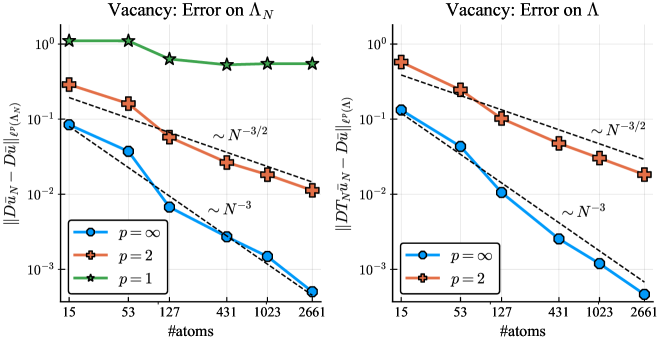
Figure 1. Numerical confirmation of the convergence rates predicted by Theorem 2.1: vacancy in bulk W (bcc), under EAM interaction.

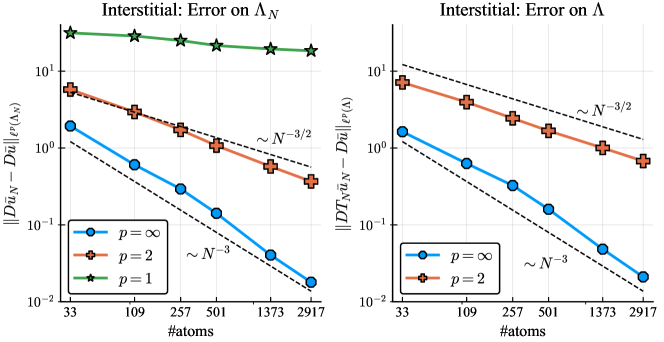
Figure 2. Numerical confirmation of the convergence rates predicted by Theorem 2.1: interstitial in bulk Cu (fcc), under Morse interaction.

The results are shown in Figures 1 and 2. Although in both cases there is a mild pre-asymptotic behaviour visible, the numerical errors follow closely the predicted rates. Note that we did not plot the errors on $\Lambda$ with respect to the $\|D\cdot\|_{\ell^{1}}$-seminorm since they are theoretically infinite but in practise due to the finite domain of the comparison solution appear to converge very slowly.

2.5. Conclusion

We haven given the first rigorous proofs of a sharp error estimate in the maximum norm (for strains) for the relaxation of a crystalline defect under artificial far-field boundary conditions.

Our restriction to point defects with periodic boundary conditions simplified one key aspect of the analysis: the sharp error estimates for the Green’s function. Indeed, there are three fundamental ingredients in our analysis: (1) an inf-sup condition which allowed us to treat general equilibria instead of only minima; (2) a sharp error estimate for the Green’s function; and (3) a Caccioppoli estimate. Our arguments for (1) and (3) seem to be generic and can likely be generalised to other situations, in particular to clamped boundary conditions for either point defects of dislocations. Extending our error estimate for the Green’s function is likely difficult in general. However, whenever this can be achieved our results should be readily extendable.

3. Proofs

In §§ 3.1–3.3, we establish auxiliary results, mostly adapting existing ideas to our setting. The proof of inf-sup stability of the periodic supercell approximation is given in § 3.4, and the proof of the sharp uniform convergence estimate in § 3.5.

3.1. Auxiliary results

An important technical tool that was used in [EOS16a] for the error analysis of the supercell approximation was a set of operators that enable us to convert functions defined in $\Lambda$ to functions defined on $\Lambda_{N}$, and vice-versa. The following results and their proofs are similar to those in [EOS16a].

Let $Q_{R}:={\sf B}(-R,R]^{d}$ and $\Lambda_{R}:=\Lambda\cap Q_{R}$ for any $R\in\mathbb{N}$. For general $R>0$ we define $Q_{R}:=Q_{\lceil R\rceil}$ and $\Lambda_{R}=\Lambda_{\lceil R\rceil}$.

Lemma 3.1 (Discrete Poincaré inequality).

There exist $r_{\rm P},R_{\rm P},C_{\rm P}>0$ such that for all $0<R_{1}<R_{2}$ with $R_{1}\geq r_{\rm P}$, $R_{2}-R_{1}\geq r_{\rm P}$, $2\leq p\leq\infty$, and $u:\Lambda_{R_{2}+R_{\rm P}}\to\mathbb{R}^{m}$ we have

$$\big{\lVert}u-\langle u\rangle_{\Lambda_{R_{2}}\setminus\Lambda_{R_{1}}}\big{\rVert}_{\ell^{p}(\Lambda_{R_{2}}\setminus\Lambda_{R_{1}})}\leq R_{2}C_{\rm P}\lVert Du\rVert_{\ell^{p}(\Lambda_{R_{2}+R_{\rm P}}\setminus\Lambda_{R_{1}-R_{\rm P}})}$$ (3.1)

$$\text{with}\qquad\langle u\rangle_{\Lambda^{\prime}}=\frac{1}{\lvert\Lambda^{\prime}\rvert}\sum_{\ell\in\Lambda^{\prime}}u(\ell).$$ (3.2)

Proof.

The restriction $R_{1}\geq r_{\rm P}$ ensures that the defect region can be ignored. On can then apply [EOS16b, Lemma 7.1] and its proof verbatim to cubes instead of balls, which states that there exists $\tilde{a}$ such that

$$\|u-\tilde{a}\|_{\ell^{2}}\lesssim R_{2}\lVert Du\rVert_{\Lambda_{R_{2}+R_{\rm P}}\setminus\Lambda_{R_{1}-R_{\rm P}}}.$$

Since $\tilde{a}=\langle u\rangle_{\Lambda_{R_{2}}\setminus\Lambda_{R_{1}}}$ minimises the left-hand side, the stated result for $p=2$ follows.

For $p=\infty$, the result is elementary. For $2<p<\infty$ it follows from the Riesz-Thorin interpolation theorem. ∎

Let $\eta_{R}\in C^{2}(\mathbb{R}^{d};[0,1])$ be a cut-off function satisfying

• $\eta_{R}(x)=1$ for $x\in Q_{4R/6}$,

• $\eta_{R}(x)=0$ for $x\in\mathbb{R}^{d}\setminus Q_{5R/6}$,

• $\lvert\nabla^{j}\eta_{R}\rvert\leq CR^{-j}$ for $j=1,2$.

Let $A_{R}:=\Lambda_{5R/6+{r_{\rm cut}}}\setminus\Lambda_{4R/6-{r_{\rm cut}}}$ be a lattice annulus, then, for $u:\Lambda_{R}\to\mathbb{R}^{m}$ and $R\geq R_{\rm T}:=\max\{2r_{\rm P},6R_{\rm P}+6{r_{\rm cut}}\}$ we can define the truncation $T_{R}u\in\dot{\mathcal{W}}^{\rm c}$ by

$$T_{R}u(\ell):=\begin{cases}\eta_{R}\big{(}u-\langle u\rangle_{A_{R}}\big{)},&\ell\in\Lambda_{R},\\ 0,&\text{otherwise.}\end{cases}$$

For $R\leq N$ we can extend $T_{R}u$ periodically with respect to $\Lambda_{N}$, in which case we call it $T_{N,R}^{\rm per}u\in\mathcal{W}^{\rm per}_{N}$. Moreover, we set $T_{N}^{\rm per}:=T_{N,N}^{\rm per}$. The following Lemma, while formulated in terms of $T_{R}$ may also be applied to $T_{N,R}^{\rm per}$ and $T_{N}^{\rm per}$.

Lemma 3.2.

There exists $C>0$ such that, for $R$ sufficiently large, $2\leq p\leq\infty$, $u:\Lambda_{R}\to\mathbb{R}^{m}$,

$$\lVert DT_{R}u\rVert_{\ell^{p}} \leq C\lVert Du\rVert_{\ell^{p}(\Lambda_{R})},$$ (3.3)

$$\lVert DT_{R}u-Du\rVert_{\ell^{p}(\Lambda_{R})} \leq C\lVert Du\rVert_{\ell^{p}(\Lambda_{R}\setminus\Lambda_{R/2})},\qquad\text{and}$$ (3.4)

$$\lVert D^{2}T_{R}u-D^{2}u\rVert_{\ell^{p}(\Lambda_{R})} \leq C\lVert D^{2}u\rVert_{\ell^{p}(\Lambda_{R}\setminus\Lambda_{R/2})}+CR^{-1}\|Du\|_{\ell^{2}(\Lambda_{R}\setminus\Lambda_{R/2})}.$$ (3.5)

Proof.

Since

$$D_{\rho}T_{R}u(\ell)=\eta_{R}(\ell+\rho)D_{\rho}u(\ell)+D_{\rho}\eta_{R}(\ell)\big{(}u(\ell)-\langle u\rangle_{A_{R}}\big{)},$$

we can use Lemma 3.1 and $R\geq R_{\rm T}$ to see that

$$\lVert DT_{R}u\rVert_{\ell^{p}} \lesssim\lVert Du\rVert_{\ell^{p}(\Lambda_{R})}+\frac{1}{R}\lVert u-\langle u\rangle_{A_{R}}\rVert_{\ell^{p}(A_{R})}\lesssim\lVert Du\rVert_{\ell^{p}(\Lambda_{R})},$$

and

$$\lVert DT_{R}u-Du\rVert_{\ell^{p}(\Lambda_{R})} \lesssim\lVert Du\rVert_{\ell^{p}(\Lambda_{R}\setminus\Lambda_{R/2})}+\frac{1}{R}\lVert u-\langle u\rangle_{A_{R}}\rVert_{\ell^{p}(A_{R})}\lesssim\lVert Du\rVert_{\ell^{p}(\Lambda_{R}\setminus\Lambda_{R/2})}.$$

This establishes (3.3) and (3.4). The proof of (3.5) is analogous. ∎

As an immediate corollary of Lemma 3.2 we obtain pointwise estimates on $T_{R}\bar{u}$.

Corollary 3.3.

Let $\bar{u}\in\dot{\mathcal{W}}^{1,2}$ be a solution to (2.3), then there exists $C>0$ such that for all $R>0,\ell\in\Lambda$ and $j=1,2$,

$$\big{|}D^{j}T_{R}\bar{u}(\ell)|\leq C(1+|\ell|)^{1-d-j}.$$ (3.6)

Proof.

The case $j=1$ is an immediate consequence of (2.6) and (3.4), case $p=\infty$. The case $j=2$ follows from (2.6) and (3.5). ∎

3.2. The Homogeneous Problem

The proof of the sharp uniform convergence rates requires sharp estimates on the Green’s function for the homogeneous supercell. In preparation for these, we first introduce some notation to effectively translate between the defective and homogeneous problems.

Recall from § 2 that $\Lambda^{\rm hom}={\sf A}\mathbb{Z}^{d}$, and analogously let $\Lambda^{\rm hom}_{N}=Q_{N}\cap\Lambda^{\rm hom}$, then we define the associated potential energies by

$$\mathcal{E}^{\rm hom}(u):=\sum_{\ell\in\Lambda^{\rm hom}}V(D^{\rm h}u(\ell)),\qquad\text{and}\qquad\mathcal{E}^{\rm hom}_{N}(u):=\sum_{\ell\in\Lambda^{\rm hom}_{N}}V(D^{\rm h}u(\ell)),$$

for, respectively, $u\in\dot{\mathcal{W}}^{\rm c}(\Lambda^{\rm hom})$ and $u\in\mathcal{W}^{\rm per}_{N}(\Lambda^{\rm hom}_{N})$. Of course, $\mathcal{E}^{\rm hom},\mathcal{E}_{N}^{\rm hom}$ have the same regularity properties as $\mathcal{E}$, listed in § 2.1.

Moreover, phonon stability (2.5) can now be written as

$$\big{\langle}\delta^{2}\mathcal{E}^{\rm hom}(0)v,v\big{\rangle}\geq c_{0}\lVert D^{\rm h}v\rVert_{\ell^{2}(\Lambda^{\rm hom})}^{2}\qquad\forall v\in\dot{\mathcal{W}}^{1,2}(\Lambda^{\rm hom}).$$

As a consequence there exists a lattice Green’s function.

Lemma 3.4.

There exists a lattice Green’s function $\mathcal{G}:\Lambda^{\rm hom}\to\mathbb{R}^{m\times m}$ satisfying

$$\big{\langle}\delta^{2}\mathcal{E}^{\rm hom}(0)(\mathcal{G}e_{i}),v\big{\rangle}=v_{i}(0)\qquad\forall v\in\dot{\mathcal{W}}^{\rm c}(\Lambda^{\rm hom}),\qquad\text{and}$$

$$\lvert(D^{\rm h})^{j}\mathcal{G}(\ell)\rvert\leq C_{j}(1+\lvert\ell\rvert)^{2-d-j}\qquad\forall j\geq 1,\ell\in\Lambda^{\rm hom}.$$ (3.7)

Furthermore, $\mathcal{G}(\ell)=\mathcal{G}(-\ell)$ for all $\ell\in\Lambda^{\rm hom}$.

Proof.

The two claims in (3.7) are proven in [EOS16a, Lemma 12]. The point symmetry of $\mathcal{G}$ is an immediate consequence of the fact that the Fourier symbol satisfies $\hat{\mathcal{G}}(k)=\hat{\mathcal{G}}(-k)$. ∎

To compare displacements $u$ of the homogeneous and the defect problem, we define linear operators $S_{N}^{\rm hom}:\mathcal{W}^{\rm per}_{N}(\Lambda_{N})\to\mathcal{W}^{\rm per}_{N}(\Lambda^{\rm hom}_{N})$ and $S_{N}^{\rm def}:\mathcal{W}^{\rm per}_{N}(\Lambda^{\rm hom}_{N})\to\mathcal{W}^{\rm per}_{N}(\Lambda_{N})$ by fixing any $\ell_{0}\in\Lambda\setminus B_{R_{\rm def}}$ and then letting

$$S_{N}^{\rm hom}u(\ell) =\begin{cases}u(\ell),&\ell\in\Lambda^{\rm hom}\setminus B_{R_{\rm def}}\\ u(\ell_{0}),&\ell\in\Lambda^{\rm hom}\cap B_{R_{\rm def}}\end{cases}\qquad\text{for }u\in\mathcal{W}^{\rm per}_{N}(\Lambda_{N}),\text{ and}$$

$$S_{N}^{\rm def}u(\ell) =\begin{cases}u(\ell),&\ell\in\Lambda\setminus B_{R_{\rm def}}\\ u(\ell_{0}),&\ell\in\Lambda\cap B_{R_{\rm def}}\end{cases}\qquad\text{for }u\in\mathcal{W}^{\rm per}_{N}(\Lambda^{\rm hom}_{N}).$$

In particular, we have the following lemma as an immediate consequence of these definitions.

Lemma 3.5.

For some $R_{\rm S}\geq R_{\rm def}+{r_{\rm cut}}$ sufficiently large, we have $D^{\rm h}S_{N}^{\rm hom}u=Du$ and $DS_{N}^{\rm def}u=D^{\rm h}u$ for $\lvert\ell\rvert>R_{\rm def}+{r_{\rm cut}}$ as well as the estimates

$$\lvert D^{\rm h}S_{N}^{\rm hom}u(\ell)\rvert \leq C\lVert Du\rVert_{\ell^{\infty}(B_{R_{\rm S}}\cap\Lambda_{N})}\qquad\forall\ell\in\Lambda^{\rm hom}\cap B_{R_{\rm def}+{r_{\rm cut}}},\quad\text{and}$$

$$\lvert DS_{N}^{\rm def}u(\ell)\rvert \leq C\lVert D^{\rm h}u\rVert_{\ell^{\infty}(B_{R_{\rm S}}\cap\Lambda_{N}^{\rm hom})}\qquad\forall\ell\in\Lambda\cap B_{R_{\rm def}+{r_{\rm cut}}}.$$

Remark 3.6.

The operators $S_{N}^{\rm def}$ and $S_{N}^{\rm hom}$ are not “optimized” for practical purposes, which likely leads to poor constants in some of our estimates. However, we only use them as a technical tool in the proofs, and are only concerned with rates. For specific defect structures, more natural operators $S_{N}^{\rm def},S_{N}^{\rm hom}$ are easily constructed.

The definition and all properties in Lemma 3.5 directly translate to analogous operators $S^{\rm hom}:\dot{\mathcal{W}}^{1,2}(\Lambda)\to\dot{\mathcal{W}}^{1,2}(\Lambda^{\rm hom})$ and $S^{\rm def}:\dot{\mathcal{W}}^{1,2}(\Lambda^{\rm hom})\to\dot{\mathcal{W}}^{1,2}(\Lambda)$ as well.

3.3. Periodic Green’s Function

We begin by recalling that phonon stability (2.5) also ensures the stability of the homogeneous periodic problem:

Lemma 3.7.

[HO12, Thm. 3.6] For all $N>0$ we have

$$\big{\langle}\delta^{2}\mathcal{E}^{\rm hom}_{N}(0)v,v\big{\rangle}\geq c_{0}\lVert D^{\rm h}v\rVert_{\ell^{2}(\Lambda^{\rm hom}_{N})}^{2}\qquad\forall v\in\mathcal{W}^{\rm per}_{N}(\Lambda^{\rm hom}_{N}).$$

In particular, for every $f:\Lambda^{\rm hom}_{N}\to\mathbb{R}^{m}$ with $\sum_{\ell\in\Lambda^{\rm hom}_{N}}f(\ell)=0$, there exists a unique $u\in\mathcal{W}^{\rm per}_{N}(\Lambda^{\rm hom}_{N})$ with $\sum_{\ell\in\Lambda^{\rm hom}_{N}}u(\ell)=0$ such that

$$\big{\langle}\delta^{2}\mathcal{E}^{\rm hom}_{N}(0)u,v\big{\rangle}=(f,v)_{\ell^{2}}\qquad\forall v\in\mathcal{W}^{\rm per}_{N}(\Lambda^{\rm hom}_{N}).$$

The periodic Green’s function $\mathcal{G}_{N}:\Lambda^{\rm hom}_{N}\to\mathbb{R}^{m\times m}$ is then defined by the equation

$$\big{\langle}\delta^{2}\mathcal{E}^{\rm hom}_{N}(0)(\mathcal{G}_{N}e_{i}),v\big{\rangle} =v_{i}(0)-\frac{1}{\lvert\Lambda^{\rm hom}_{N}\rvert}\sum_{\ell\in\Lambda^{\rm hom}_{N}}v_{i}(\ell)\qquad\forall v\in\mathcal{W}^{\rm per}_{N}(\Lambda^{\rm hom}_{N})$$

$$=:\big{(}\delta_{0}e_{i}-\frac{1}{\lvert\Lambda^{\rm hom}_{N}\rvert}{\bf 1}e_{i},v\big{)}_{\ell^{2}}$$

To estimate the decay of $\mathcal{G}_{N}$ we relate $\mathcal{G}$ and $\mathcal{G}_{N}$.

Lemma 3.8.

For every $j\geq 1$ there exist constants $C_{1},C_{2}$, independent of $N$, such that

$$\big{\|}(D^{\rm h})^{j}\mathcal{G}-(D^{\rm h})^{j}\mathcal{G}_{N}\big{\|}_{\ell^{\infty}(\Lambda^{\rm hom}_{N})} \leq C_{1}N^{2-d-j},\qquad\text{and in particular}$$

$$|(D^{\rm h})^{j}\mathcal{G}_{N}(\ell)| \leq C_{2}(1+{\rm dist}(\ell,2N{\sf B}\mathbb{Z}^{d}))^{2-d-j}\qquad\forall\,\ell\in\Lambda^{\rm hom}.$$

Proof.

First, we note that

$$\sum_{\ell\in\Lambda^{\rm hom}}(D^{\rm h})^{j}\mathcal{G}(\ell)=0\qquad\forall j\geq 3,$$ (3.8)

which is straightforward to prove due to the gradient structure. (For $j<3$, $(D^{\rm h})^{j}\mathcal{G}(\ell)$ does not decay fast enough to even define this sum.)

Fix $i\in\{1,\dots,m\},\rho_{1},\rho_{2},\rho_{3}\in\mathcal{R}$ and let

$$w(\ell):=\sum_{z\in\mathbb{Z}^{d}}D_{\rho_{1}}D_{\rho_{2}}D_{\rho_{3}}\mathcal{G}(\ell+2N{\sf B}z)e_{i}\qquad\forall\ell\in\Lambda^{\rm hom}.$$

Due to the decay (3.7), the sum exists. Moreover, $w$ is $\Lambda^{\rm hom}_{N}$-periodic, satisfies

$$\big{\langle}\delta^{2}\mathcal{E}^{\rm hom}_{N}(0)w,v\big{\rangle}=(D_{\rho_{1}}D_{\rho_{2}}D_{\rho_{3}}\delta_{0}e_{i},v)_{\ell^{2}}$$

and according to (3.8) also $\sum_{\ell\in\Lambda^{\rm hom}_{N}}w(\ell)=0$.

Since $D_{\rho_{1}}D_{\rho_{2}}D_{\rho_{3}}\mathcal{G}_{N}e_{i}$ solves the same equation and has average zero as well, we can therefore deduce that

$$(D^{\rm h})^{3}\mathcal{G}_{N}=\sum_{z\in\mathbb{Z}^{d}}(D^{\rm h})^{3}\mathcal{G}(\ell+2N{\sf B}z).$$

Consequently, for $j\geq 3$ and $\ell\in\Lambda^{\rm hom}_{N}$,

$$\big{\lvert}(D^{\rm h})^{j}\mathcal{G}(\ell)-(D^{\rm h})^{j}\mathcal{G}_{N}(\ell)\big{\rvert} =\Big{\lvert}\sum_{z\in\mathbb{Z}^{d}\setminus\{0\}}(D^{\rm h})^{j}\mathcal{G}(\ell+2N{\sf B}z)\Big{\rvert}$$

$$\lesssim\sum_{z\in\mathbb{Z}^{d}\setminus\{0\}}(1+\lvert\ell+2N{\sf B}z\rvert)^{2-d-j}$$

$$\lesssim N^{2-d-j}\sum_{z\in\mathbb{Z}^{d}\setminus\{0\}}\lvert{\sf B}^{-1}\ell/N+2z\rvert^{2-d-j}$$

$$\lesssim N^{2-d-j},$$

where we used that the series converges due to $j\geq 3$ and the estimate is uniform due to the uniform lower bound $\lvert{\sf B}^{-1}\ell/N+2z\rvert\geq 1$.

It remains to establish the estimate for $j=1,2$, which we will obtain from a discrete Poincaré inequality: For all $g:\Lambda^{\rm hom}_{N}\to\mathbb{R}^{m}$ we clearly have

$$\lvert g(x)-g(y)\rvert\leq CN\lVert D^{\rm h}g\rVert_{\ell^{\infty}(\Lambda^{\rm hom}_{N})}\qquad\forall x,y\in\Lambda^{\rm hom}_{N}$$

hence it immediately follows that

$$\|g-\langle g\rangle_{\Lambda^{\rm hom}_{N}}\|_{\ell^{\infty}(\Lambda^{\rm hom}_{N})}\leq CN\|D^{\rm h}g\|_{\ell^{\infty}(\Lambda^{\rm hom}_{N})},$$ (3.9)

where $\langle g\rangle_{\Lambda^{\rm hom}_{N}}=\lvert\Lambda^{\rm hom}_{N}\rvert^{-1}\sum_{\ell\in\Lambda^{\rm hom}_{N}}g(\ell)$.

Fix $\rho,\sigma\in\mathcal{R}$ and let $C_{N}:=\langle D_{\rho}D_{\sigma}\mathcal{G}-D_{\rho}D_{\sigma}\mathcal{G}_{N}\rangle_{\Lambda^{\rm hom}_{N}}$, then combining the estimate for $j=3$ and (3.9) we obtain

$$\|D_{\rho}D_{\sigma}\mathcal{G}-D_{\rho}D_{\sigma}\mathcal{G}_{N}\|_{\ell^{\infty}(\Lambda^{\rm hom}_{N})} \leq\|D_{\rho}D_{\sigma}\mathcal{G}-D_{\rho}D_{\sigma}\mathcal{G}_{N}-C_{N}\|_{\ell^{\infty}(\Lambda^{\rm hom}_{N})}+|C_{N}|$$

$$\lesssim N\|D^{\rm h}D_{\rho}D_{\sigma}\mathcal{G}-D^{\rm h}D_{\rho}D_{\sigma}\mathcal{G}_{N}\|_{\ell^{\infty}(\Lambda^{\rm hom}_{N})}+|C_{N}|$$

$$\lesssim N^{-d}+\big{|}C_{N}\big{|}.$$

It thus remains to estimate $C_{N}$.

Periodicity of $\mathcal{G}_{N}$ implies that $\langle D_{\rho}D_{\sigma}\mathcal{G}_{N}\rangle_{\Lambda^{\rm hom}_{N}}=0$, hence,

$$C_{N}=\lvert\Lambda^{\rm hom}_{N}\rvert^{-1}\sum_{\ell\in\Lambda^{\rm hom}_{N}}D_{\rho}D_{\sigma}\mathcal{G}(\ell).$$

Using discrete summation by parts we see that

$$|C_{N}| =|\Lambda^{\rm hom}_{N}|^{-1}\bigg{|}\sum_{\ell\in(\Lambda^{\rm hom}_{N}+\rho)\setminus\Lambda^{\rm hom}_{N}}D_{\sigma}\mathcal{G}(\ell)-\sum_{\ell\in\Lambda^{\rm hom}_{N}\setminus(\Lambda^{\rm hom}_{N}+\rho)}D_{\sigma}\mathcal{G}(\ell)\bigg{|}$$

$$\lesssim N^{-d}N^{d-1}N^{1-d}=N^{-d}.$$

This establishes the result for $j=2$.

To prove the estimate for $j=1$, we can repeating the same argument on just $D_{\rho}\mathcal{G}-D_{\rho}\mathcal{G}_{N}$, to obtain

$$\|D_{\rho}\mathcal{G}-D_{\rho}\mathcal{G}_{N}\|_{\ell^{\infty}(\Lambda^{\rm hom}_{N})}\lesssim N^{1-d}+N^{-d}\bigg{|}\sum_{\ell\in\Lambda^{\rm hom}_{N}}D_{\rho}\mathcal{G}(\ell)\bigg{|}.$$

From here on, however, we need to argue differently and in particular exploit cancellations due to symmetries in the Green’s function, to avoid logarithmic terms. To that end, we define the point symmetric extension

$$\Lambda^{\rm hom}_{s,N}=\Lambda^{\rm hom}\cap{\sf B}[-N,N]^{d}$$

of $\Lambda^{\rm hom}$ (i.e., $-\Lambda^{\rm hom}_{s,N}=\Lambda^{\rm hom}_{s,N}$) and use $\mathcal{G}(\ell)=\mathcal{G}(-\ell)$ to calculate

$$\bigg{|}\sum_{\ell\in\Lambda^{\rm hom}_{N}}D_{\rho}\mathcal{G}(\ell)\bigg{|} \lesssim\bigg{|}\sum_{\ell\in\Lambda^{\rm hom}_{s,N}}D_{\rho}\mathcal{G}(\ell)\bigg{|}+N^{1-d}N^{d-1}$$

$$=\bigg{|}\sum_{\ell\in(\Lambda^{\rm hom}_{s,N}+\rho)\setminus\Lambda^{\rm hom}_{s,N}}\mathcal{G}(\ell)-\sum_{\ell\in\Lambda^{\rm hom}_{s,N}\setminus(\Lambda^{\rm hom}_{s,N}+\rho)}\mathcal{G}(\ell)\bigg{|}+1$$

$$=\bigg{|}\sum_{\ell\in(\Lambda^{\rm hom}_{s,N}+\rho)\setminus\Lambda^{\rm hom}_{s,N}}\mathcal{G}(-\ell)-\sum_{\ell\in\Lambda^{\rm hom}_{s,N}\setminus(\Lambda^{\rm hom}_{s,N}+\rho)}\mathcal{G}(\ell)\bigg{|}+1$$

$$=\bigg{|}\sum_{\ell\in(\Lambda^{\rm hom}_{s,N}-\rho)\setminus\Lambda^{\rm hom}_{s,N}}\mathcal{G}(\ell)-\sum_{\ell\in\Lambda^{\rm hom}_{s,N}\setminus(\Lambda^{\rm hom}_{s,N}+\rho)}\mathcal{G}(\ell)\bigg{|}+1$$

$$=\bigg{|}\sum_{\ell\in(\Lambda^{\rm hom}_{s,N})\setminus(\Lambda^{\rm hom}_{s,N}+\rho)}\mathcal{G}(\ell-\rho)-\mathcal{G}(\ell)\bigg{|}+1$$

$$\leq\sum_{\ell\in(\Lambda^{\rm hom}_{s,N})\setminus(\Lambda^{\rm hom}_{s,N}+\rho)}\lvert D\mathcal{G}(\ell)\rvert+1$$

$$\lesssim N^{d-1}N^{1-d}+1$$

$$\lesssim 1.$$

Hence, $\|D_{\rho}\mathcal{G}-D_{\rho}\mathcal{G}_{N}\|_{\ell^{\infty}(\Lambda^{\rm hom}_{N})}\lesssim N^{1-d}$. ∎

3.4. Inf-sup stability

The first step in the error analysis of the supercell approximation is to establish that it inherits inf-sup stability (2.4). This is a generalisation of the result in [EOS16b, Theorem 7.7] that the supercell approximation inherits positivity of the Hessian operator, a more stringent notion of stability suitable only for minimisers.

In the stability analysis it is convenient to factor out constants from $\dot{\mathcal{W}}^{1,2}$ and $\mathcal{W}^{\rm per}_{N}$. Let $\mathcal{W}_{0}\subset\dot{\mathcal{W}}^{1,2}$ and $\mathcal{W}_{N,0}\subset\mathcal{W}^{\rm per}_{N}$ denote the $m$-dimensional subspaces of all constant functions, then we define

$$\dot{W}^{1,2}:=\dot{\mathcal{W}}^{1,2}/\mathcal{W}_{0}\qquad\text{and}\qquad W^{\rm per}_{N}:=\mathcal{W}^{\rm per}_{N}/\mathcal{W}_{N,0}.$$

The associated equivalence classes of a function $u\in\dot{\mathcal{W}}^{1,2},\mathcal{W}^{\rm per}_{N}$ are denoted by $[u]$, however, whenever an expression is independent of constants, we will abuse notation and identify $[u]\equiv u$, for example, $D[u]=Du$. The inner products associated with $\dot{W}^{1,2},W^{\rm per}_{N}$ are then defined by

$$(v,w)_{\dot{W}^{1,2}}=(Dv,Dw)_{\ell^{2}(\Lambda)}\qquad\text{and}\qquad(v,w)_{W^{\rm per}_{N}}=(Dv,Dw)_{\ell^{2}(\Lambda_{N})},$$

and turn these factor spaces into Hilbert spaces.

For the proofs of the following results, recall that we made the standing assumption (2.5) that the homogeneous reference lattice is stable. Without this (standard) assumption the negative eigenspace identified in Lemma 3.9 need not be finite-dimensional, and this would make our strategy infeasible.

Lemma 3.9.

(i) For all $u\in\dot{\mathcal{W}}^{1,2}$, there exists a subspace $\mathcal{W}_{1}\subset\dot{\mathcal{W}}^{1,2}$ with finite co-dimension such that

$$\big{\langle}\delta^{2}\mathcal{E}(u)v,v\big{\rangle}\geq{\textstyle\frac{1}{2}}c_{0}\|Dv\|_{\ell^{2}}^{2}\qquad\forall v\in\mathcal{W}_{1}.$$

(ii) If, in addition, $u$ is inf-sup stable (2.4) then there exists $c_{1}>0$ and an orthogonal decomposition $\dot{W}^{1,2}=W_{-}\oplus W_{+}$ with ${\rm dim}(W_{-})=q$ finite and

$$\pm\big{\langle}\delta^{2}\mathcal{E}(u)v,v\big{\rangle}\geq c_{1}\|Dv\|_{\ell^{2}}^{2}\qquad\forall v\in W_{\pm}.$$

Moreover, we may choose $W_{-}={\rm span}\{\psi_{1},\dots,\psi_{q}\}$, where $\psi_{j}$ are eigenfunctions of $\delta^{2}\mathcal{E}(u)$ in the $\dot{W}^{1,2}$ sense.

Proof.

(i) Let $\mathcal{W}_{R}:=\{v\in\dot{\mathcal{W}}^{1,2}\,|\,Dv|_{B_{R}}=0\}$, then for $v\in\mathcal{W}_{R}$, and for $R>R_{\rm def}+{r_{\rm cut}}$,

$$\big{|}\big{\langle}\delta^{2}\mathcal{E}(u)v,v\big{\rangle}-\big{\langle}\delta^{2}\mathcal{E}^{\rm hom}(0)S^{\rm hom}v,S^{\rm hom}v\big{\rangle}\big{|} \lesssim\sum_{\ell\in\Lambda\setminus B_{R}}\big{|}\nabla^{2}V(Du(\ell))-\nabla^{2}V(0)\big{|}\,|Dv(\ell)|^{2}$$

$$\lesssim\|Du\|_{\ell^{\infty}(\Lambda\setminus B_{R})}\,\|Dv\|_{\ell^{2}}^{2}\lesssim\epsilon_{R}\|Dv\|_{\ell^{2}}^{2}.$$

where $\epsilon_{R}\to 0$ as $R\to\infty$ since $Du\in\ell^{2}$. Phonon stability (2.5) then implies that, for $R$ sufficiently large,

$$\big{\langle}\delta^{2}\mathcal{E}(u)v,v\big{\rangle}\geq{\textstyle\frac{1}{2}}c_{0}\|Dv\|_{\ell^{2}}^{2}.$$

Since the co-dimension of $\mathcal{W}_{R}$ is finite, statement (i) follows with $\mathcal{W}_{1}=\mathcal{W}_{R}$.

(ii) Since $\delta^{2}\mathcal{E}(u)$ is a symmetric, continuous bilinear map on $\dot{W}^{1,2}$, there is a unique linear, self-adjoint, bounded operator $A(u)\in L(\dot{W}^{1,2})$ with $\langle\delta^{2}\mathcal{E}(u)v,w\rangle=(A(u)v,w)_{\dot{W}^{1,2}}$ for all $v,w\in\dot{W}^{1,2}$. Inf-sup stability (2.4) implies that $A(u)$ is an isomorphism. Thus, the spectrum of $A(u)$ is real, bounded, and bounded away from $0$. In light of (i), the spectral subspace of the negative part of the spectrum is finite dimensional. The negative part of the spectrum thus consists of only finitely many eigenvalues (with multiplicity) $\lambda_{1}\leq\cdots\leq\lambda_{q}$ and associated orthonormal eigenfunctions $\psi_{j}$, $1\leq j\leq q$. Define $\mathcal{W}_{-}:={\rm span}\{\psi_{1},\dots,\psi_{q}\}$ to be that spectral subspace, and $\mathcal{W}_{+}$ the orthogonal complement of $\mathcal{W}_{-}$, then (ii) follows. ∎

Lemma 3.10.

Suppose that $u\in\dot{\mathcal{W}}^{1,2}$ is inf-sup stable (2.4) then, for $N$ sufficiently large,

$$\inf_{\begin{subarray}{c}v\in\mathcal{W}^{\rm per}_{N}\\ \|Dv\|_{\ell^{2}}=1\end{subarray}}\sup_{\begin{subarray}{c}w\in\mathcal{W}^{\rm per}_{N}\\ \|Dw\|_{\ell^{2}}=1\end{subarray}}\big{\langle}\delta^{2}\mathcal{E}_{N}(T_{N}^{\rm per}u)v,w\big{\rangle}\geq\min(c_{0}/8,c_{1}/4).$$ (3.10)

Proof.

Let $u_{N}=T_{N}^{\rm per}u$, $H_{N}:=\delta^{2}\mathcal{E}_{N}(u_{N})$ and $H:=\delta^{2}\mathcal{E}(u)$. We will consider the orthogonal decomposition $W^{\rm per}_{N}=W_{N,+}\oplus W_{N,-}$, where

$$W_{N,-}={\rm span}\big{\{}T_{N,N/2}^{\rm per}\psi_{j}\,|\,j=1,\dots,q\big{\}}$$

with $\psi_{j}$ the negative eigenfunctions of $H$ (cf. Lemma 3.9(ii)) and $W_{N,+}$ its orthogonal complement. We will prove that $H_{N}$ is uniformly positive on $W_{N,+}$ and uniformly negative on $W_{N,-}$, which implies the stated inf-sup condition (3.10).

If $v_{N}\in W_{N,-}$ then $v_{N}=T_{N,N/2}^{\rm per}v$ for some $v\in W_{-}$. In particular, $Dv_{N}(\ell)=0$ for $\ell\in\Lambda_{N}\setminus\Lambda_{N/2}$ and since also $Du_{N}(\ell)=Du(\ell)$ for all $\ell\in\Lambda_{N/2}$ we obtain

$$\big{\langle}H_{N}T_{N,N/2}^{\rm per}v,T_{N,N/2}^{\rm per}v\big{\rangle} =\sum_{\ell\in\Lambda_{N/2}}\nabla^{2}V_{\ell}(Du_{N}(\ell))\big{[}DT_{N,N/2}^{\rm per}v,DT_{N,N/2}^{\rm per}v\big{]}$$

$$=\sum_{\ell\in\Lambda_{N/2}}\nabla^{2}V_{\ell}(Du(\ell))\big{[}DT_{N/2}v,DT_{N/2}v\big{]}$$

$$=\big{\langle}HT_{N/2}v,T_{N/2}v\big{\rangle}$$

$$=\big{\langle}Hv,v\big{\rangle}+\big{\langle}H\big{(}T_{N/2}v+v\big{)},T_{N/2}v-v\big{\rangle}$$

$$\leq-c_{1}\|v\|_{\dot{W}^{1,2}}^{2}+C\|v\|_{\dot{W}^{1,2}}\|T_{N/2}v-v\|_{\dot{W}^{1,2}}.$$

Since $\|T_{N/2}\psi_{j}-\psi_{j}\|_{\dot{W}^{1,2}}\to 0$ for all $1\leq j\leq q$, for a given $\epsilon$ we obtain $\|T_{N/2}v-v\|_{\dot{W}^{1,2}}\leq\epsilon\|v\|_{\dot{W}^{1,2}}$ for all $N$ large enough uniformly in $v\in W_{-}$. For $\epsilon$ small enough,

$$\langle H_{N}v_{N},v_{N}\rangle\leq(-c_{1}+C\epsilon)\|v\|_{\dot{W}^{1,2}}^{2}\leq\frac{-c_{1}+C\epsilon}{(1+\epsilon)^{2}}\|v_{N}\|_{W^{\rm per}}^{2}\leq-c_{1}/2\|v_{N}\|_{W^{\rm per}}^{2}.$$ (3.11)

Next we prove uniform positivity of $H_{N}$ on $W_{N,+}$, the complement of $W_{N,-}$. This is a straightforward variation of the argument when $W_{N,-}=\{0\}$ treated in [EOS16b, Theorem 7.7]. First, we take an increasing sequence $N_{k}$ such that

$$\lim_{k\to\infty}\min_{\begin{subarray}{c}v\in W_{N_{k},+}\\ \lVert v\rVert_{W^{\rm per}_{N_{k}}}=1\end{subarray}}\langle H_{N_{k}}v,v\rangle=\liminf_{N\to\infty}\min_{\begin{subarray}{c}v\in W_{N,+}\\ \lVert v\rVert_{W^{\rm per}_{N}}=1\end{subarray}}\langle H_{N}v,v\rangle,$$

and then choose

$$v_{k}\in\arg\min_{\begin{subarray}{c}v\in W_{N_{k},+}\\ \lVert v\rVert_{W^{\rm per}_{N_{k}}}=1\end{subarray}}\langle H_{N_{k}}v,v\rangle.$$

Next, we want to choose a second sequence $R_{k}\uparrow\infty$, $R_{k}\leq N_{k}/4$, and decompose

$$v_{k}=a_{k}+b_{k}:=T_{N_{k},R_{k}}^{\rm per}v_{k}+(I-T_{N_{k},R_{k}}^{\rm per})v_{k}.$$

According to [EOS16b, Lemma 7.8] and [EOS16b, Proof of Theorem 7.7] , one can find a subsequence of $(N_{k})_{k\in\mathbb{N}}$ (not relabelled) and $R_{k}\uparrow\infty$ sufficiently slowly such that

$$\langle H_{N_{k}}a_{k},b_{k}\rangle\to 0\qquad\text{and}\qquad(D_{\rho}a_{k},D_{\sigma}b_{k})_{\ell^{2}(\Lambda_{N_{k}})}\to 0\qquad\text{as }k\to\infty,$$ (3.12)

for all $\rho,\sigma\in\mathcal{R}$. We split

$$\langle H_{N_{k}}v_{k},v_{k}\rangle=\langle H_{N_{k}}a_{k},a_{k}\rangle+2\langle H_{N_{k}}a_{k},b_{k}\rangle+\langle H_{N_{k}}b_{k},b_{k}\rangle.$$

According to (3.12), the cross-term vanishes in the limit, $\langle H_{N_{k}}a_{k},b_{k}\rangle\to 0$.

Since the support of $Db_{k}$ does not intersect the defective region it is easy to see that

$$\langle H_{N_{k}}b_{k},b_{k}\rangle=\big{\langle}\delta^{2}\mathcal{E}_{N_{k}}^{\rm hom}(u_{N_{k}}^{\rm hom})S_{N_{k}}^{\rm hom}b_{k},S_{N_{k}}^{\rm hom}b_{k}\big{\rangle}.$$

where $u_{N_{k}}^{\rm hom}:=S_{N_{k}}^{\rm hom}u_{N_{k}}$. Next, we observe that

$$\Big{|}\big{\langle}\big{[}\delta^{2}\mathcal{E}_{N_{k}}^{\rm hom}(u_{N_{k}}^{\rm hom})-\delta^{2}\mathcal{E}_{N_{k}}^{\rm hom}(0)\big{]}S_{N_{k}}^{\rm hom}b_{k},S_{N_{k}}^{\rm hom}b_{k}\big{\rangle}\Big{|}$$

$$=~{} \bigg{|}\sum_{\ell\in\Lambda_{N_{k}}^{\rm hom}\setminus\Lambda_{R_{k}/2}^{\rm hom}}\Big{(}\nabla^{2}V(Du_{N_{k}}^{\rm hom}(\ell))-\nabla^{2}V(0)\Big{)}\big{[}DS_{N_{k}}^{\rm hom}b_{k}(\ell),DS_{N_{k}}^{\rm hom}b_{k}(\ell)\big{]}\bigg{|}$$

$$\lesssim~{} \epsilon_{k}\|DS_{N_{k}}^{\rm hom}b_{k}\|_{\ell^{2}(\Lambda^{\rm per,hom}_{N_{k}})}^{2}\lesssim\epsilon_{k}\|b_{k}\|_{W^{\rm per}_{N_{k}}}^{2},$$

where, according to (3.4),

$$\epsilon_{k} :=\max_{\ell\in\Lambda_{N_{k}}^{\rm hom}\setminus\Lambda_{R_{k}/2}^{\rm hom}}\big{|}D^{\rm h}u_{N_{k}}^{\rm hom}(\ell)\big{|}$$

$$=\max_{\ell\in\Lambda_{N_{k}}\setminus\Lambda_{R_{k}/2}}\big{|}DT_{N_{k}}u(\ell)\big{|}$$

$$\leq\lVert DT_{N_{k}}u\rVert_{\ell^{2}(\Lambda_{N_{k}}\setminus\Lambda_{R_{k}/2})}$$

$$\leq\lVert Du\rVert_{\ell^{2}(\Lambda_{N_{k}}\setminus\Lambda_{R_{k}/2})}+\lVert DT_{N_{k}}u-Du\rVert_{\ell^{2}(\Lambda_{N_{k}})}$$

$$\lesssim\lVert Du\rVert_{\ell^{2}(\Lambda_{N_{k}}\setminus\Lambda_{R_{k}/2})}$$

$$\to 0\quad\text{ as }k\to\infty.$$

In particular, using Lemma 3.7, we obtain

$$\langle H_{N_{k}}b_{k},b_{k}\rangle \geq\big{\langle}\delta^{2}\mathcal{E}_{N_{k}}^{\rm hom}(0)S_{N_{k}}^{\rm hom}b_{k},S_{N_{k}}^{\rm hom}b_{k}\big{\rangle}-C\epsilon_{k}\|b_{k}\|_{W^{\rm per}_{N_{k}}}^{2}$$

$$\geq(c_{0}-C\epsilon_{k})\|b_{k}\|_{W^{\rm per}_{N_{k}}}^{2}\geq c_{0}/2\|b_{k}\|_{W^{\rm per}_{N_{k}}}^{2},$$ (3.13)

for $k$ sufficienty large.

Finally, since $Da_{k}$ are supported in $\Lambda_{{N_{k}}/4}$ we have

$$(T_{N_{k}}a_{k},\psi_{j})_{\dot{W}^{1,2}} =(a_{k},T_{N_{k},N_{k}/2}^{\rm per}\psi_{j})_{W^{\rm per}_{N_{k}}}+(T_{N_{k}}a_{k},(I-T_{N_{k}/2})\psi_{j})_{\dot{W}^{1,2}}$$

$$=(v_{k},T_{N_{k},N_{k}/2}^{\rm per}\psi_{j})_{W^{\rm per}_{N_{k}}}-(b_{k},T_{N_{k},N_{k}/2}^{\rm per}\psi_{j})_{W^{\rm per}_{N_{k}}}+0$$

$$=-(b_{k},T_{N_{k},N_{k}/2}^{\rm per}\psi_{j})_{W^{\rm per}_{N_{k}}}$$

Hence, for all $j=1,\dots,q$,

$$\lvert(T_{N_{k}}a_{k},\psi_{j})_{\dot{W}^{1,2}}\rvert =\lvert(b_{k},T_{N_{k},N_{k}/2}^{\rm per}\psi_{j})_{W^{\rm per}_{N_{k}}}\rvert$$

$$\lesssim\max_{j}\lVert D\psi_{j}\rVert_{\ell^{2}(\Lambda_{N_{k}}\setminus\Lambda_{R_{k}/2})}=:\gamma_{k}\to 0.$$

Writing $T_{N_{k}}a_{k}=a_{k}^{+}+a_{k}^{-}$ with $a_{k}^{\pm}\in W_{\pm}$, Lemma 3.9(ii) implies

$$\langle H_{N_{k}}a_{k},a_{k}\rangle=\langle HT_{N_{k}}a_{k},T_{N_{k}}a_{k}\rangle\geq c_{1}\|a_{k}^{+}\|_{\dot{W}^{1,2}}^{2}-C\|a_{k}^{-}\|_{\dot{W}^{1,2}}^{2}\geq c_{1}\|a_{k}\|_{W^{\rm per}_{N_{k}}}^{2}-C\gamma_{k}.$$ (3.14)

In summary, combining (3.14) with (3.13) and recalling again (3.12) we conclude that, for $k$ sufficiently large,

$$\inf_{\begin{subarray}{c}v\in W_{N_{k},+}\\ \lVert v\rVert_{W^{\rm per}_{N_{k}}}=1\end{subarray}}\langle H_{N_{k}}v,v\rangle =\langle H_{N_{k}}v_{k},v_{k}\rangle$$

$$\geq\min(c_{0}/2,c_{1})\big{(}\|a_{k}\|_{W^{\rm per}_{N_{k}}}^{2}+\|b_{k}\|_{W^{\rm per}_{N_{k}}}^{2}\big{)}-C\gamma_{k}$$

$$=\min(c_{0}/2,c_{1})\|v_{k}\|_{W^{\rm per}_{N_{k}}}^{2}-2\min(c_{0}/2,c_{1})\,(a_{k},b_{k})_{W^{\rm per}_{N_{k}}}-C\gamma_{k}$$

$$\geq\min(c_{0}/4,c_{1}/2).$$

Due to the choice of the $N_{k}$, this means that for all $N$ large enough,

$$\inf_{\begin{subarray}{c}v\in W_{N,+}\\ \lVert v\rVert_{W^{\rm per}_{N}}=1\end{subarray}}\langle H_{N}v,v\rangle \geq\min(c_{0}/8,c_{1}/4).\qed$$

As an immediate corollary of the inf-sup stability of the supercell approximation we obtain a convergence result in the energy norm.

Theorem 3.11.

Let $\bar{u}\in\dot{\mathcal{W}}^{1,2}$ be an inf-sup stable solution to (2.3), then there exist $C>0$ such that, for $N$ sufficiently large, there are $\bar{u}_{N}\in\mathcal{W}^{\rm per}_{N}$ satisfying (2.7) as well as

$$\big{\|}D\bar{u}_{N}-DT_{N}^{\rm per}\bar{u}\big{\|}_{\ell^{2}}\lesssim N^{-d/2}.$$

Proof.

The proof of this result is identical to that of [EOS16a, Thm. 2.6], replacing positivity of $\delta^{2}\mathcal{E}_{N}(T_{N}^{\rm per}\bar{u})$ with the new inf-sup stability result provided by Lemma 3.10. ∎

3.5. Uniform Convergence

Let $\bar{u}\in\dot{\mathcal{W}}^{1,2}$ be an inf-sup stable solution to (2.3), then according to Theorem 3.11 there exists $\bar{u}_{N}\in\mathcal{W}^{\rm per}_{N}$ solving (2.7) and satisfying

$$\lVert D\bar{u}-D\bar{u}_{N}\rVert_{\ell^{2}}\lesssim N^{-d/2}.$$

Throughout the remainder of this section, we fix $\bar{u}$ and the sequences $\bar{u}_{N}$, as well as $v_{N}:=T_{N}^{\rm per}\bar{u},\bar{u}_{N}^{\rm hom}:=S_{N}^{\rm hom}\bar{u}_{N},v_{N}^{\rm hom}:=S_{N}^{\rm hom}v_{N}$,

$$e_{N}:=\bar{u}_{N}-v_{N},\qquad\text{and}\qquad e_{N}^{\rm hom}:=\bar{u}_{N}^{\rm hom}-v_{N}^{\rm hom}.$$

In particular we will also assume implicitly that $N$ is sufficiently large so that the existence of $\bar{u}_{N}$ is guarenteed. We will prove a uniform convergence rate for $e_{N}$, from which Theorem 2.1 will readily follow.

Recall from the definition of $T_{N}^{\rm per}$ and from Corollary 3.3 that

$$\begin{split}Dv_{N}=D\bar{u}\quad&\text{ in }\Lambda_{N/2},\qquad\text{and}\\ |D^{j}v_{N}|\lesssim N^{1-d-j}\quad&\text{ in }\Lambda_{N}\setminus\Lambda_{N/3},\quad j=1,2.\end{split}$$ (3.15)

First, we use our Green’s function estimates to obtain an implicit estimate for $De_{N}$.

Lemma 3.12.

There exists $r_{0},C_{1}>0$ such that for all $\ell\in\Lambda_{N}\setminus\Lambda_{r_{0}}$

$$|De_{N}(\ell)|\leq C_{1}\bigg{(}N^{-d}+\sum_{m\in\Lambda_{N}}\big{(}{\rm dist}(\ell-m,2N{\sf B}\mathbb{Z}^{d})+1\big{)}^{-d}(1+|m|)^{-d}|De_{N}(m)|\bigg{)}.$$

Proof.

Let

$$\sigma_{N}^{\rm hom}(\ell) :=\big{(}\nabla V(D^{\rm h}\bar{u}_{N}^{\rm hom}(\ell))-\nabla V(D^{\rm h}v_{N}^{\rm hom}(\ell))\big{)}\chi_{B_{R_{\rm def}+{r_{\rm cut}}}}(\ell),$$

$$\sigma_{N}^{\rm def}(\ell) :=\big{(}\nabla V_{\ell}(D\bar{u}_{N}(\ell))-\nabla V_{\ell}(Dv_{N}(\ell))\big{)}\chi_{R_{\rm def}+{r_{\rm cut}}}(\ell),$$

$$f_{N}^{\rm bdry}(\ell) :=-{\rm Div}\nabla V_{\ell}(Dv_{N}(\ell))$$

$$:=\sum_{\rho\in-\mathcal{R}_{\ell}}\nabla_{D_{\rho}}V_{\ell-\rho}(Dv_{N}(\ell-\rho))-\sum_{\rho\in\mathcal{R}_{\ell}}\nabla_{D_{\rho}}V_{\ell}(Dv_{N}(\ell)),$$

where $\nabla_{D_{\rho}}V_{\ell}(Du(\ell))=\partial V_{\ell}(Du(\ell))/\partial D_{\rho}u(\ell)$.

Then a straightforward algebraic manipulation shows that, for any $w\in\mathcal{W}^{\rm per}_{N}(\Lambda^{\rm hom}_{N})$,

$$\big{\langle}\delta\mathcal{E}_{N}^{\rm hom}(\bar{u}_{N}^{\rm hom}) -\delta\mathcal{E}_{N}^{\rm hom}(v_{N}^{\rm hom}),w\big{\rangle}$$

$$=(\sigma_{N}^{\rm hom},Dw)_{\ell^{2}(\Lambda_{N}^{\rm hom})}-(\sigma_{N}^{\rm def},DS_{N}^{\rm def}w)_{\ell^{2}(\Lambda_{N})}-(f_{N}^{\rm bdry},S_{N}^{\rm def}w)_{\ell^{2}(\Lambda_{N})}.$$

Furthermore, for $N\geq 6r_{\rm cut}$, it is straightforward to establish that

$$\lvert\sigma_{N}^{\rm hom}(\ell)\rvert \lesssim\lvert D^{\rm h}e_{N}^{\rm hom}(\ell)\rvert \forall\ell\in\Lambda^{\rm hom}_{N}\cap B_{R_{\rm def}+{r_{\rm cut}}},$$ (3.16)

$$\lvert\sigma_{N}^{\rm def}(\ell)\rvert \lesssim\lvert De_{N}(\ell)\rvert, \forall\ell\in\Lambda_{N}\cap B_{R_{\rm def}+{r_{\rm cut}}},\qquad\text{and}$$ (3.17)

$$\lvert f_{N}^{\rm bdry}(\ell)\rvert \lesssim\begin{cases}0,&\ell\in\Lambda_{N/3},\\ N^{-d-1},&\ell\in\Lambda_{N}\setminus\Lambda_{N/3}.\end{cases}$$ (3.18)

The first two estimates follow simply from the fact that $V,V_{\ell}\in C^{4}$ while (3.18) follows from the second-order difference structure of $f_{N}^{\rm bdry}(\ell)$ and (3.15).

Furthermore, Taylor expansions of $\delta\mathcal{E}_{N}^{\rm hom}(\bar{u}_{N}^{\rm hom})$ and $\delta\mathcal{E}_{N}^{\rm hom}(v_{N}^{\rm hom})$ about $0$, and some elementary manipulations yield

$$\big{\langle}\delta\mathcal{E}_{N}^{\rm hom}(\bar{u}_{N}^{\rm hom})-\delta\mathcal{E}_{N}^{\rm hom}(v_{N}^{\rm hom}),w\big{\rangle}$$

$$=\big{\langle}\delta^{2}\mathcal{E}_{N}^{\rm hom}(0)e_{N}^{\rm hom},w\rangle+\int_{0}^{1}\big{\langle}\big{[}\delta^{2}\mathcal{E}_{N}^{\rm hom}(tv_{N}^{\rm hom})-\delta^{2}\mathcal{E}_{N}^{\rm hom}(0)\big{]}e_{N}^{\rm hom},w\big{\rangle}\,dt$$

$$\hskip 105.2751pt+\int_{0}^{1}\big{\langle}\big{[}\delta^{2}\mathcal{E}_{N}^{\rm hom}(t\bar{u}_{N}^{\rm hom})-\delta^{2}\mathcal{E}_{N}^{\rm hom}(tv_{N}^{\rm hom})\big{]}u_{N}^{\rm hom},w\big{\rangle}\,dt$$

$$=\big{\langle}\delta^{2}\mathcal{E}_{N}^{\rm hom}(0)e_{N}^{\rm hom},w\rangle$$

$$\qquad+\int_{0}^{1}\int_{0}^{t}\big{\langle}\big{[}\delta^{3}\mathcal{E}_{N}^{\rm hom}(sv_{N}^{\rm hom})e_{N}^{\rm hom},v_{N}^{\rm hom},w\big{\rangle}\,dt\,ds$$

$$\qquad+\int_{0}^{1}\int_{0}^{t}\big{\langle}\delta^{3}\mathcal{E}_{N}^{\rm hom}((t-s)v_{N}^{\rm hom}+s\bar{u}_{N}^{\rm hom})e_{N}^{\rm hom},e_{N}^{\rm hom}+v_{N}^{\rm hom},w\big{\rangle}\,dt\,ds.$$

We test with $w(n)=D^{\rm h}G_{N}(n-\ell)$ then

$$|(D^{\rm h})^{j}w(n)|\lesssim\big{(}{\rm dist}(\ell-m,2N{\sf B}\mathbb{Z}^{d})+1\big{)}^{1-d-j},$$ (3.19)

hence, for $\lvert\ell\rvert>R_{\rm def}+{r_{\rm cut}}$, we obtain

$$|De_{N}(\ell)| =\lvert D^{\rm h}e_{N}^{\rm hom}(\ell)\rvert=\big{\langle}\delta^{2}\mathcal{E}_{N}^{\rm hom}(0)(\bar{u}_{N}^{\rm hom}-v_{N}^{\rm hom}),w\rangle$$

$$\lesssim\big{|}\big{(}\sigma_{N}^{\rm hom},D^{\rm h}w\big{)}_{\ell^{2}(\Lambda^{\rm hom}_{N})}\big{|}+\big{|}\big{(}\sigma_{N}^{\rm def},DS_{N}^{\rm def}w\big{)}_{\ell^{2}(\Lambda_{N})}\big{|}+\big{\lvert}(f_{N}^{\rm bdry},S_{N}^{\rm def}w)_{\ell^{2}(\Lambda_{N})}\big{\rvert}$$

$$\quad+\sum_{m\in\Lambda^{\rm hom}_{N}}|De_{N}^{\rm hom}(m)|^{2}\,|Dw(n)|$$

$$\quad+\sum_{m\in\Lambda_{N}^{\rm hom}}\lvert De_{N}^{\rm hom}(m)\rvert\lvert Dw(m)\rvert\,|Dv_{N}^{\rm hom}(m)|$$

$$=:{\rm T}_{1}+{\rm T}_{2}+{\rm T}_{3}+{\rm T}_{4}+{\rm T}_{5}.$$

The fifth term is already of the form we require: We can employ (3.19) to bound $Dw$ and (3.15) to bound $Dv_{N}^{\rm hom}$. Furthermore, we use Lemma 3.5 to bound $De_{N}^{\rm hom}$ by $De_{N}$ to arrive at

$${\rm T}_{5} \lesssim\sum_{m\in\Lambda_{N}^{\rm hom}}\lvert De_{N}(m)\rvert\big{(}{\rm dist}(\ell-m,2N{\sf B}\mathbb{Z}^{d})+1\big{)}^{-d}(1+|m|)^{-d}$$

for $\lvert\ell\rvert>2R_{\rm S}$. Using, (3.18) in combination with (3.19), as well as using $\lVert De_{N}^{\rm hom}\rVert_{\ell^{2}}\leq N^{-d/2}$ we get ${\rm T}_{3}+{\rm T}_{4}\lesssim N^{-d}.$ Finally, for ${\rm T}_{1}$ and ${\rm T}_{2}$ and again, $\lvert\ell\rvert>2R_{\rm S}$, we use (3.16) and (3.17) to estimate

$${\rm T}_{1}+{\rm T}_{2} \lesssim\sum_{m\in\Lambda^{\rm hom}_{N}\cap B_{R_{\rm S}}}\lvert D^{\rm h}e_{N}^{\rm hom}(m)\rvert\lvert D^{2}\mathcal{G}(\ell-m)\rvert+\sum_{m\in\Lambda_{N}\cap B_{R_{\rm S}}}\lvert De_{N}(m)\rvert\lvert DS^{\rm def}D^{\rm h}\mathcal{G}(\ell-m)\rvert$$

$$\lesssim\sum_{k\in\Lambda^{\rm hom}_{N}\cap B_{R_{\rm S}}}\sum_{m\in\Lambda_{N}\cap B_{R_{\rm S}}}\lvert De_{N}(m)\rvert\lvert D^{2}\mathcal{G}(\ell-k)\rvert$$

$$\lesssim\sum_{m\in\Lambda_{N}^{\rm hom}\cap B_{R_{\rm S}}}\lvert De_{N}(m)\rvert\big{(}{\rm dist}(\ell-m,2N{\sf B}\mathbb{Z}^{d})+1\big{)}^{-d}.\qed$$

Next, we prove a discrete Caccioppoli estimate.

Lemma 3.13.

There exist $r_{1},C_{2}>0$ such that, for $r_{1}\leq r\leq N/4$,

$$\|De_{N}\|_{\ell^{2}(\Lambda_{r/2})}\leq C_{2}\|De_{N}\|_{\ell^{2}(\Lambda_{2r}\setminus\Lambda_{r/2})}.$$

Proof.

Inf-sup stability of $v_{N}$ established in Lemma 3.10 and the convergence $\|De_{N}\|_{\ell^{2}}\to 0$ (cf. Theorem 3.11) imply that there exists $c_{1}>0$ such that, for all $N$ sufficiently large,

$$\sup_{\begin{subarray}{c}w\in\mathcal{W}^{\rm per}_{N}\\ \|Dw\|_{\ell^{2}}=1\end{subarray}}\int_{0}^{1}\big{\langle}\delta^{2}\mathcal{E}_{N}(v_{N}+te_{N})z,w\big{\rangle}\,dt\geq c_{1}\lVert Dz\rVert_{\ell^{2}}\qquad\forall z\in\mathcal{W}^{\rm per}_{N}.$$

In the rest of this proof we will write $\sup_{w}=\sup_{w\in\mathcal{W}^{\rm per}_{N},\|Dw\|_{\ell^{2}}=1}$ . Fix $r>0$ and insert $z=T_{N,r}^{\rm per}e_{N}$ in the inf-sup condition, then we can use the fact that the supports of $Dz$ and $D(I-T_{N,2r}^{\rm per})w$ do not overlap to write

$$\|Dz\|_{\ell^{2}} \lesssim\sup_{w}\int_{0}^{1}\big{\langle}\delta^{2}\mathcal{E}_{N}(v_{N}+te_{N})z,w\big{\rangle}\,dt$$

$$=\sup_{w}\int_{0}^{1}\big{\langle}\delta^{2}\mathcal{E}_{N}(v_{N}+te_{N})z,T_{N,2r}^{\rm per}w\big{\rangle}\,dt$$

$$=\sup_{w}\bigg{(}\int_{0}^{1}\big{\langle}\delta^{2}\mathcal{E}_{N}(v_{N}+te_{N})(T_{N,r}^{\rm per}-I)e_{N},T_{N,2r}^{\rm per}w\big{\rangle}\,dt$$

$$\hskip 85.35826pt+\big{\langle}\delta\mathcal{E}_{N}(\bar{u}_{N})-\delta\mathcal{E}_{N}(v_{N}),T_{N,2r}^{\rm per}w\big{\rangle}\bigg{)}.$$

We clearly have $\langle\delta\mathcal{E}_{N}(\bar{u}_{N}),T_{N,2r}^{\rm per}w\rangle=0$. Moreover,

$$\big{\langle}\delta\mathcal{E}_{N}(v_{N}),T_{N,2r}^{\rm per}w\big{\rangle} =\sum_{\ell\in\Lambda_{2r}}\nabla V_{\ell}(Dv_{N}(\ell))\big{[}DT_{N,2r}^{\rm per}w\big{]}$$

$$=\sum_{\ell\in\Lambda_{2r}}\nabla V_{\ell}(D\bar{u}(\ell))\big{[}DT_{2r}w\big{]}$$

$$=\big{\langle}\delta\mathcal{E}(\bar{u}),T_{2r}w\big{\rangle}=0,$$

which leaves us with only the term

$$\|Dz\|_{\ell^{2}} \lesssim\sup_{w}\int_{0}^{1}\big{\langle}\delta^{2}\mathcal{E}_{N}(v_{N}+te_{N})(T_{N,r}^{\rm per}-I)e_{N},T_{N,2r}^{\rm per}w\big{\rangle}\,dt.$$

Since $DT_{N,2r}^{\rm per}w=0$ in $\Lambda\setminus\Lambda_{2r}$ we can estimate this further by

$$\|Dz\|_{\ell^{2}} \lesssim\sup_{w}\sum_{\ell\in\Lambda_{2r}}\big{|}D(T_{N,r}^{\rm per}-I)e_{N}(\ell)\big{|}\,\big{|}DT_{N,2r}^{\rm per}w(\ell)\big{|}$$

$$\lesssim\sup_{w}\|D(T_{N,r}^{\rm per}-I)e_{N}(\ell)\|_{\ell^{2}(\Lambda_{2r})}\,\|DT_{N,2r}^{\rm per}w\|_{\ell^{2}}$$

$$\lesssim\|D(T_{N,r}^{\rm per}-I)e_{N}(\ell)\|_{\ell^{2}(\Lambda_{2r})},$$

where, in the last estimate, we used Lemma 3.2 to bound $\|DT_{N,2r}^{\rm per}w\|_{\ell^{2}}\lesssim\|Dw\|_{\ell^{2}}\lesssim 1$.

Using Lemma 3.2 a second time we finally deduce that

$$\|De_{N}\|_{\ell^{2}(\Lambda_{r/2})} \leq\|Dz\|_{\ell^{2}(\Lambda_{N})}\lesssim\|D(T_{r}-I)e_{N}(\ell)\|_{\ell^{2}(\Lambda_{2r})}$$

$$\lesssim\|D(T_{r}-I)e_{N}(\ell)\|_{\ell^{2}(\Lambda_{r})}+\|De_{N}(\ell)\|_{\ell^{2}(\Lambda_{2r}\setminus\Lambda_{r})}$$

$$\lesssim\|De_{N}(\ell)\|_{\ell^{2}(\Lambda_{2r}\setminus\Lambda_{r/2})}.\qed$$

Our main result, Theorem 2.1, will follow from the next intermediate result, which is of independent interest.

Theorem 3.14.

Under the conditions of Theorem 2.1,

$$\lVert De_{N}\rVert_{\ell^{\infty}(\Lambda_{N})}\lesssim N^{-d}.$$

Proof.

Let $\omega(r):=\|De_{N}\|_{\ell^{\infty}(\Lambda_{N}\setminus\Lambda_{r})}$, then according to Lemma 3.12, for $r\geq r_{0}$,

$$\omega(r) \lesssim N^{-d}+\sup_{\ell\in\Lambda_{N}\setminus\Lambda_{r}}\sum_{m\in\Lambda_{N}}\big{(}{\rm dist}(\ell-m,2N{\sf B}\mathbb{Z}^{d})+1\big{)}^{-d}(1+\lvert m\rvert)^{-d}\lvert De_{N}(m)\rvert$$

$$\lesssim N^{-d}+\omega(r)\sup_{\ell\in\Lambda_{N}\setminus\Lambda_{r}}\sum_{m\in\Lambda_{N}\setminus\Lambda_{r}}\big{(}{\rm dist}(\ell-m,2N{\sf B}\mathbb{Z}^{d})+1\big{)}^{-d}(1+|m|)^{-d}$$

$$\hskip 59.75095pt+\sup_{\ell\in\Lambda_{N}\setminus\Lambda_{r}}\sum_{m\in\Lambda_{r}}(1+\lvert\ell-m\rvert)^{-d}(1+\lvert m\rvert)^{-d}\lvert De_{N}(m)\rvert$$

$$\lesssim N^{-d}+\omega(r)\sup_{\ell\in\Lambda_{N}\setminus\Lambda_{r}}\sum_{z\in\{-1,0,1\}^{d}}\sum_{m\in\Lambda_{N}}(1+\lvert\ell-m-2N{\sf B}z\rvert)^{-d}(1+|m|)^{-d}$$

$$\hskip 59.75095pt+\sup_{\ell\in\Lambda_{N}\setminus\Lambda_{r}}\Big{(}\sum_{m\in\Lambda_{r}}(1+\lvert\ell-m\rvert)^{-2d}(1+\lvert m\rvert)^{-2d}\Big{)}^{1/2}\lVert De_{N}\rVert_{\ell^{2}(\Lambda_{r})}$$

$$\lesssim N^{-d}+\omega(r)\sup_{\ell\in\Lambda_{N}\setminus\Lambda_{r}}\max_{z\in\{-1,0,1\}^{d}}|\ell-2N{\sf B}z|^{-d}\log|\ell-2N{\sf B}z|$$

$$\hskip 59.75095pt+\sup_{\ell\in\Lambda_{N}\setminus\Lambda_{r}}|\ell|^{-d}\lVert De_{N}\rVert_{\ell^{2}(\Lambda_{r})}$$

$$\lesssim N^{-d}+\omega(r)r^{-d}\log(r)+r^{-d}\lVert De_{N}\rVert_{\ell^{2}(\Lambda_{r})}.$$

Here we used that, for $|\ell|\geq 2$,

$$\sum_{m\in\Lambda}(1+\lvert\ell-m\rvert)^{-d}(1+|m|)^{-d} \lesssim|\ell|^{-d}\log|\ell|,\qquad\text{ and}$$

$$\sum_{m\in\Lambda}(1+\lvert\ell-m\rvert)^{-2d}(1+|m|)^{-2d} \lesssim|\ell|^{-2d}.$$

We apply the Caccioppoli inequality, Lemma 3.13, further restricting to $r_{1}/2\leq r\leq N/8$, to continue to estimate

$$\omega(r) \lesssim N^{-d}+\omega(r)r^{-d}\log(r)+\lVert De_{N}\rVert_{\ell^{2}(\Lambda_{4r}\setminus\Lambda_{r})}r^{-d}$$

$$\leq C_{3}\big{(}N^{-d}+\omega(r)r^{-d/2}\big{)}.$$

For $r_{2}:=(2C_{3})^{2/d}$ and $r\geq r_{3}:=\max\{r_{0},r_{1},r_{2}\}$, we thus find $\omega(r)\leq 2C_{3}N^{-d}$. That is, we have proven that $|De_{N}(\ell)|\lesssim N^{-d}$ for all $\ell\in\Lambda_{N}\setminus\Lambda_{r_{3}}$, where $r_{3}$ is independent of $N$.

It thus remains only to consider $\ell\in\Lambda_{r_{3}}$, a finite subdomain. Applying Lemma 3.13 a second time we obtain

$$\lvert De_{N}(\ell)\rvert\leq\lVert De_{N}\rVert_{\ell^{2}(\Lambda_{r_{3}})}\lesssim\lVert De_{N}\rVert_{\ell^{2}(\Lambda_{4r_{3}}\setminus\Lambda_{r_{3}})}\lesssim\omega(r_{3})\lesssim N^{-d}.\qed$$

Proof of Theorem 2.1.

We split

$$\|D\bar{u}_{N}-D\bar{u}\|_{\ell^{\infty}(\Lambda_{N})} \leq\|De_{N}\|_{\ell^{\infty}(\Lambda_{N})}+\|Dv_{N}-D\bar{u}\|_{\ell^{\infty}(\Lambda_{N})}$$

$$\lesssim N^{-d}+\|Dv_{N}-D\bar{u}\|_{\ell^{\infty}(\Lambda_{N})},$$

where we used Theorem 3.14. For $\ell\in\Lambda_{N/2}$, $Dv_{N}(\ell)-D\bar{u}(\ell)=0$. Conversely, for $\ell\in\Lambda_{N}\setminus\Lambda_{N/2}$, (3.15) and (2.6) imply that

$$|Dv_{N}(\ell)-D\bar{u}(\ell)|\leq|Dv_{N}(\ell)|+|D\bar{u}(\ell)|\lesssim N^{-d}.\qed$$

References

- [BDO18] J. Braun, M. H. Duong, and C. Ortner. Thermodynamic limit of the transition rate of a crystalline defect. ArXiv e-prints, 1810.11643, 2018.
- [BHO] J. Braun, T. Hudson, and C. Ortner. in preparation.
- [CO17] H. Chen and C. Ortner. QM/MM methods for crystalline defects. Part 2: Consistent energy and force-mixing. Multiscale Model. Simul., 15(1), 2017.
- [DLO10] Matthew Dobson, Mitchell Luskin, and Christoph Ortner. Stability, instability, and error of the force-based quasicontinuum approximation. Arch. Ration. Mech. Anal., 197(1):179–202, 2010.
- [Dol99] Georg Dolzmann. Optimal convergence for the finite element method in Campanato spaces. Mathematics of Computation of the American Mathematical Society, 68(228):1397–1427, 1999.
- [EOS16a] V. Ehrlacher, C. Ortner, and A. V. Shapeev. Analysis of boundary conditions for crystal defect atomistic simulations. Archive for Rational Mechanics and Analysis, 222(3):1217–1268, 2016.
- [EOS16b] V. Ehrlacher, C. Ortner, and A. V. Shapeev. Analysis of boundary conditions for crystal defect atomistic simulations. ArXiV e-prints, 1306.5334v4, 2016.
- [HO12] T. Hudson and C. Ortner. On the stability of Bravais lattices and their Cauchy–Born approximations. M2AN Math. Model. Numer. Anal., 46:81–110, 2012.
- [LM13] Jianfeng Lu and Pingbing Ming. Convergence of a Force-Based hybrid method in three dimensions. Commun. Pure Appl. Math., 66(1):83–108, 2013.
- [LOSK16] X. H. Li, C. Ortner, A. Shapeev, and B. Van Koten. Analysis of blended atomistic/continuum hybrid methods. Numer. Math., 134, 2016.
- [OLOVK18] Derek Olson, Xingjie Li, Christoph Ortner, and Brian Van Koten. Force-based atomistic/continuum blending for multilattices. Numer. Math., July 2018.
- [OS08] Christoph Ortner and Endre Süli. Analysis of a quasicontinuum method in one dimension. M2AN Math. Model. Numer. Anal., 42(1):57–91, 2008.
- [PKM+16] D. Packwood, J. Kermode, L. Mones, N. Bernstein, J. Woolley, N. I. M. Gould, C. Ortner, and G. Csanyi. A universal preconditioner for simulating condensed phase materials. J. Chem. Phys., 144, 2016.
- [RS82] Rolf Rannacher and Ridgway Scott. Some optimal error estimates for piecewise linear finite element approximations. Math. Comput., 38(158):437–445, 1982.
- [Wal98] Duane C Wallace. Thermodynamics of Crystals. Courier Corporation, 1998.
- [WZLH13] J. Wang, Y.L. Zhou, M. Li, and Q. Hou. A modified W-W interatomic potential based on ab initio calculations. Modelling and Simulation in Materials Science and Engineering, 22(1), 2013.